| Issue |
A&A
Volume 696, April 2025
|
|
|---|---|---|
| Article Number | A115 | |
| Number of page(s) | 14 | |
| Section | The Sun and the Heliosphere | |
| DOI | https://doi.org/10.1051/0004-6361/202453527 | |
| Published online | 09 April 2025 | |
Three-dimensional He+ pick-up ion velocity distribution functions observed with STEREO-A PLASTIC
1
TNG Stadtnetz GmbH, Kiel, Germany
2
Christian Albrechts University, Kiel, Germany
⋆ Corresponding author; This email address is being protected from spambots. You need JavaScript enabled to view it.
Received:
19
December
2024
Accepted:
5
March
2025
Abstract
Context. Freshly injected interstellar pick-up ion (PUIs) are expected to exhibit a simple, torus-shaped velocity distribution function (VDF). The PUI velocity in the solar wind (SW) frame depends on the velocity of the interstellar neutral (ISN) population at the pick-up position.
Aims. We directly compare PUI VDFs measured by the plasma and suprathermal ion composition (PLASTIC) instrument over the full orbit of solar terestrial relations observatory-ahead (STEREO-A).
Methods. The STEREO-PLASTIC-A PUI observations were re-analysed, and instrumental effects of the limited field of view (FOV) were accounted for. We then defined a new position-independent velocity measure for PUIs that takes the local direction of the ISN inflow into account. The resulting new PUI velocity measure corrects thereby for the position-dependent contribution of the ISN velocity. Each position in the orbit of STEREO can be reached by ISNs following one of two trajectories, which we call primary and secondary trajectories. Therein, ISNs following the primary trajectory have a higher probability to reach the location before they are ionised than particles following the secondary trajectory. Our new PUI velocity measure can be applied based on the assumption that all particles followed the primary trajectory or that all particles followed the secondary trajectory. Pitch-angle distributions were then analysed depending on the magnetic field azimuthal angle for different orbital positions and different values of the PUI velocity measure.
Results. The new velocity measure, ϖinj, p, shows an approximately constant cut-off over the complete orbit of STEREO-A. A torus signature is visible everywhere. Therein, a broadening of the torus signature outside the focusing cone and crescent regions and for lower ϖinj, p is observed. In addition, we illustrate the symmetry between the primary and secondary ISN trajectory in the vicinity of the focusing cone.
Conclusions. A torus signature associated with freshly injected PUIs is visible over the complete orbit of STEREO-A with increased density in the focusing cone. At least remnants of a torus signature remain for lower values of the PUI velocity measure. The new velocity measure also prepares for PUI studies with Solar Orbiter.
Key words: plasmas / Sun: heliosphere / solar wind / ISM: general
© The Authors 2025
 Open Access article, published by EDP Sciences, under the terms of the Creative Commons Attribution License (https://creativecommons.org/licenses/by/4.0), which permits unrestricted use, distribution, and reproduction in any medium, provided the original work is properly cited.
This article is published in open access under the Subscribe to Open model. This email address is being protected from spambots. You need JavaScript enabled to view it. to support open access publication.
1. Introduction
The SW is a continuous flow of charged particles that emanate from the Sun (Biermann 1957). The particles constitute a magnetised plasma that governs the interplanetary space surrounding the Sun. Surrounding the SW is the local interstellar medium (LISM), which itself is a magnetised plasma and therefore cannot mix with the SW.
Interstellar PUIs are a species of particles found in the SW, which are not of solar origin, but are implanted in the SW. They originate from ISNs that inflow into the heliosphere. The trajectory of an ISN is mainly governed by two forces: Gravitation from the Sun (and to a for the purpose of this paper negligible degree from the larger planets of the solar system; Axford 1972; Vasyliunas & Siscoe 1976), and radiation pressure from solar ultraviolet photons (UVs; Tarnopolski & Bzowski 2009; Shestakova 2015). Radiation pressure is relevant for protons, for example, but it is almost negligible for He particles. He exhibit at 1 AU (astronomical unit) a prominent focusing cone behind the Sun (Gloeckler et al. 2004) and a crescent feature on the other side (McComas et al. 2004; Drews et al. 2012; Sokół et al. 2016). Without the influence of radiation pressure, the trajectories of ISNs are solutions to the two-body problem and therefore elliptical trajectories (Axford 1972).
Because these trajectories were computed before by several studies, this study focuses on the consequences of the ISN velocities before pick-up on the PUI velocity characteristics. The method we used to compute the trajectories and velocities is found in Appendix B. A consequence of the symmetry of the two-body problem is the formation of the focusing cone. Here, enhanced ISNs densities are expected (Axford 1972). Yet, neutral particles cannot be measured by a majority of space-borne instruments, which are built for the detection of charged particles. Still, the measurement of ISN particles or neutral particles in the heliosphere in general has led to the discovery of the interstellar boundary explorer (IBEX) ribbon (McComas et al. 2009). Indirectly, through PUIs, ISNs can still be detected: On its trajectory through the heliosphere, an ISN is likely to become ionised, most prominently, for He by photoionisation by ultraviolet radiation. Therefore, the ionisation probability increases with decreasing distance to the Sun. Through ionisation, the former neutrals are subjected to the local magnetic field Lorentz force, which causes them to gyrate around the magnetic field lines. These are embedded into the outward-propagating SW. Hence, the particles are picked up by the SW and called PUIs.
Compared to ions heavier than H or He in the SW from the Sun, most PUIs undergo only a single or, more rarely, a double ionisation (Axford 1972; Gloeckler et al. 1993, 1995; Möbius et al. 1985; Gloeckler & Geiss 1998; Gloeckler et al. 2000). Therefore, PUIs can in many cases be distinguished from the SW by their charge state. This study focuses on He+ PUIs. Since most He of solar origin is fully ionised in the SW, the charge state is already a good indicator for a PUI. However, for He2+ PUIs, characteristics of the VDF are the only information based on which we can distinguish their in situ observations from ions of the SW. For He+ PUIs, compared to different ion species, their distinct mass-per-charge ratio of 4 is also well distinguished from different ion species, which makes them an ideal candidate for studies with time-of-flight mass spectrometers (Sect. 2.1).
Figure 1 depicts the injection of a PUI in 3D velocity space for different magnetic field configurations. The initial ISN has a velocity of vISN on its Keplerian trajectory. However, in the SW frame (green arrow) that transports the magnetic field, the initial velocity of a newly created PUI is the difference between the ISN velocity and the frame velocity vSW. It is important to note that the vSW is not necessarily the correct velocity of the frame of transport of charged particles in the SW. It might be shifted by a velocity of the magnitude of the local Alfvén velocity (Němeček et al. 2020). However, a detailed analysis of the transport velocity is beyond the scope of this work and might even require better precision than can be provided with the employed instruments. In the transporting frame, the vector vSW − vISN is the origin of the gyration around the local magnetic field (the difference between the blue ISN speed and the green SW speed in Fig. 1). This results in a circular trajectory in velocity space with a radius of v⊥ with  , where
  is a unit vector parallel to the magnetic field (amber ring in Fig. 1). In addition to the gyration, the PUI may move parallel to the magnetic field with a velocity of v∥. The pitch angle, that is, the inclination angle of the particle gyration trajectory with respect to the local magnetic field, is a function of the angle between the local magnetic field and the initial PUI velocity, and it can be expressed as α = arctan(v⊥/v∥). Each circle centred around the local magnetic field in velocity space is a collection of velocities of the same pitch angle. Under the assumption that multiple PUIs are injected with the same or similar pitch angles at slightly different times, a collection of gyrating particles at different phases is found. For freshly created PUIs, a torus distribution is therefore expected in velocity space.
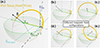 |
Fig. 1. three-dimensional (3D) visualisation of a freshly injected PUIs in velocity space in the SW frame of reference. The green arrows represent the SW bulk velocity, the black arrows show the local magnetic field, the blue arrows show the ISN velocity, and the amber ring shows the initial PUI VDF. The green hemisphere is a cut-out of the sphere of the entirety of velocities of fresh PUIs at the depicted setup of the SW velocity and ISN velocity. The different visualisations depict in total five different magnetic field configurations, and the other parameters are kept constant. |
It is often assumed, however, that during transport in the SW, the pitch angle distribution quickly becomes less anisotropic (Vasyliunas & Siscoe 1976; Isenberg 1997). Previous studies with one-dimensional (1D) velocity data observed anisotropies (Moebius et al. 1995; Gloeckler & Geiss 1998). In contrast, clear signs of remains of torus-shaped distributions were observed and were matched with the magnetic field orientation in two-dimensional (2D) velocity data with the plasma and suprathermal ion composition (PLASTIC) instrument (Drews et al. 2015) on board the solar terestrial relations observatory-ahead (STEREO-A) and with the magnetospheric multiscale (MMS; Starkey et al. 2021). For a more detailed analysis, we employed 3D velocity information. The studies mentioned above also emphasised that there is an important factor for understanding the relation between PUIs and the ISNs from which they originate: The strength of transport effects in the SW, or as a proxy, the timescale of isotropisation in the SW.
A method for classifying the timescale of transport modifications is to compare freshly created PUIs with PUIs that were injected in the SW earlier. After pick-up, the newly generated PUIs gyrate around the magnetic field direction. The interplanetary magnetic field itself moves with the SW velocity. Therefore, when we neglect for the moment the initial ISN velocity, the relative velocity of the newly generated PUI to the SW frame is also the SW velocity (Gloeckler & Geiss 1998; Gloeckler et al. 2004; Drews et al. 2015). Since the initial velocity of PUIs is thereby known, the velocity vPUI can be employed as a qualifier for the recentness of ionisation of a PUI. Hence, the quantity ϖSW with
 (1)
(1)
was introduced for the analysis of PUI velocities (Gloeckler & Geiss 1998). Neglecting the ISN velocity, a fresh PUI is expected with a ϖSW = 1. When the ISN velocity is not neglected, fresh PUIs deviate from ϖSW = 1, wherein the difference (or shift) is a function of the position-dependent ISN velocity and therefore a function of orbital position. Möbius et al. (2015), Taut et al. (2018) employed this shift in PUI velocities to determine the inflow direction of the LISM. It is necessary to point out that Möbius et al. (2015) measured the position-dependent shift in PUI velocities from ϖSW spectra. Hence, the resulting shift is intrinsically a result of the directional difference between vISN and vSW. In contrast, we propose a method that directly accounts for the velocity shift with the 3D velocity information instead of with absolute velocities. To this end, Sect. 3 presents a new PUI velocity measure, ϖinj, p, that includes the local ISN velocity. The clear advantage of a velocity measure that accounts for the ISN velocity is that the VDFs at different orbital positions are disentangled from the position-dependent velocity shift and can therefore be more readily compared than without the ISN velocity. Moreover, for any point in the heliosphere, at least two ISN trajectories intersect under the consideration of orbital mechanics with this point (compare Appendix B). Hence, their influence on the PUI signatures can be investigated. Table 1 provides an overview on different PUI velocity measures and their properties.
Overview of the PUI relative velocity measures.
It is again important to point out that in contrast to Drews et al. (2015), for example, we employed full 3D vector information for both vPUI and vSW in an effort to increase the analysis precision and mitigate possible projection errors. Section 4 revisits the results from Drews et al. (2015) based on the new velocity measure, and Sect. 5 uses the new velocity measure to compare the PUI pitch-angle distribution along the full orbit of STEREO-A.
2. Preparation of STEREO-A PLASTIC Pulse Height Analysis (PHA) data
For a measurement of full PUI VDFs and an assessment of their qualitative shape, specific requirements need to be met by the measuring instrument. Firstly, the instrument needs to determine the mass and charge state of each particle. Secondly, it is necessary that the instrument is capable of measuring particles with significantly lower densities than the proton part of the SW. Thirdly, it is necessary to not only measure 1D absolute velocities, but to gain full 3D vector information of the velocities. The combination of these criteria is met by the PLasma And SupraThermal Ion Composition (PLASTIC; Galvin et al. 2008) instrument on board the Solar TErestrial RElations Observatory-Ahead (STEREO-A).
2.1. He+ PHA data
Figure 2 shows an overview of the structure of PLASTIC (top half) together with an example of typical observations for a single energy-per-charge step (bottom half of Fig. 2). PLASTIC is a time-of-flight mass spectrometer and a cylindrical top-hat sensor (see the cross-sections in Fig. 2). It was originally designed to measure protons and heavy ions with a lateral FOV of almost 360°. The instrument is segmented into three sections that were built for different requirements: The Solar Wind Sector (SWS) observes in the direction of the incoming SW and not only features a triple coincidence measurement (electrostatic analyser, time-of-flight, and SSD), but also the capability of elevation angle measurements with an electrostatic deflection system. Herein, a range of 45° is separated into 32 bins. In the SWS, lateral direction resolution is achieved with a resistive anode with 32 bins as well (channels 16-48) in a range of 45° within the SWS. The other two sections were built with a coarser binning in the longitudinal incident angle, do not feature an elevation angle measurement, and are partly not equipped with SSDs. Hence, we only employed SWS data.
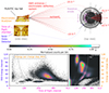 |
Fig. 2. Top left: Rendered side view of PLASTIC (cut in half). The entrance of the top hat of the cylindrical sensor is separated into two parts: The solar wind sector (SWS), and the wide-angle partition. Within the top hat, the electrostatic analyser is housed. In the lower parts of the instrument, the time-of-flight chamber and an solid state detector (SSD) are found. An example trajectory that enters the tophat is plotted in turquoise. Top right: Superimposed top-view cross-sections of PLASTIC. At the top, the entrance system is visible. At lower layers, the resistive anode and solid-state detectors are found. In purple we show the resistive anode channels, corresponding to the incident directions from the SWS aperture on the opposite side of the instrument. Bottom: Histograms of PLASTIC pulse-height analysis data from 2009. The left histogram shows the SSD energy channel as a function of the time-of-flight channel, wherein only events contribute that occur during energy-per-charge step 44. The dashed grey line shows the expected positions of He+ and He2+ for all energy-per-charge steps. The right histogram shows the energy-per-charge step as a function of time-of-flight channel. The dashed white line shows the expected average position of He+. The right histogram is normalised to individual maxima of time-of-flight slices. |
The pitch angles covered by the position channels of the resistive anode are depicted in Fig. 4a (which summarises all pre-processing steps and is discussed in more detail in Sect. 2.3) as a function of the magnetic field azimuthal angle. Unfortunately, the instrument measures particles with an asymmetric efficiency (Keilbach 2023). Hence, we considered data from the φ < 0° half of SWS (channels between 16 and 32) and the φ > 0° half of SWS (channels between 32 and 48) separately, as if they originated from different sensors. We mainly focused on the φ < 0° half. The consequence is that the pitch-angle coverage as a function of magnetic field orientation becomes smaller for each instrument half, as shown in the mapping of the position channels to pitch angles in Fig. 4a.
The data from the position channels in proximity to channel 32 are also to be viewed with additional care because particles are scattered at a support structure in the centre of the instrument. Hence, channel 32 is practically a blind spot of the instrument (the events that occur there are likely due to scattering in the instrument), and channels next to it are likely affected by edge effects.
The instrument steps through 128 energy-per-charge settings every minute. Per energy-per-charge step, the electrostatic deflection system sweeps once through its 32 settings. Since at the energy-per-charge steps corresponding to protons the flux through the instrument increases drastically, the SWS entrance system is split into a larger and a smaller opening (main channel and small channel). When a flux threshold is reached, the instrument switches between these two channels. We expect the ions of interest in the main channel. Further, PHA events were pre-selected by an on-board logic, with priorities defined by ground-calibrated priority classes. The idea behind this was to prevent that under the limited telemetry of the instrument, the most common particle species in the SW take most of the available telemetry to the detriment of the less common heavier ions. For the purpose of correcting the number of events, the instrument accumulates statistics of the total number of events per priority class in cycles of 5 minutes. Hence, instrumental data are available with a cadence of 5 minutes.
The identification of He+ particles from the PHA data was described in detail in Keilbach (2023). The peaks of both He+ and He2+ in SSD energy versus time-of-flight histograms (as an example, the histogram for energy-per-charge step 44 is shown in the bottom left corner of Fig. 2) are tracked while the contributing data are filtered by energy-per-charge step. As an overview, a histogram of energy-per-charge versus time of flight is depicted in the bottom right corner of Fig. 2. This leads to a model function for the positions of the ions, which is then employed to separate the He+ ions from the remaining PHA data. After the ions and therefore their mass-per-charge m/q are identified, the absolute velocity v is obtained from the energy-per-charge æ = (m/q)⋅v2/2. A vector quantity is gained from the absolute velocity from the information of the electrostatic deflection step and the resistive anode. The selection and calibration approach we applied was explained in more detail by Keilbach (2023). In 2015, STEREO-A was rotated by 180° around the sun-pointing axis. We focused on the time period prior to this flip of STEREO-A, that is, we analysed data from 2008–2015. Interplanetary coronal mass ejections (ICMEs) and stream interaction regions (SIRs) were removed from the data set based on the respective available Jian et al. (2013, 2018) and Jian et al. (2019) lists.
To reduce contamination of protons and O6+ events, additional filtering was required. The mass-per-charge of He+ is 4 amu/e, the mass-per-charge of O6+ is 2.7 amu/e, and the mass-per-charge of protons is 1 amu/e. For the contaminating elements, the mass-per-charge is therefore considerably lower than for He+. When a proton or O6+ is misidentified as He+, its velocity computed from energy-per-charge is accordingly considerably slower than that of the SW bulk because unfittingly, the mass-per-charge of 4 amu/e is assumed for the velocity computation. For interstellar PUIs, velocities in the spacecraft frame are expected that range to at least twice the SW velocity. This leads to the criterion that all particles with wSW := |vPUI − vSW|/|vSW|< 0.5 and vPUI − vSW/|vSW|< 0 were labelled as likely contamination and were disregarded. In addition, instrumental deficiencies and asymmetries were identified. Their treatment was also described by Keilbach (2023).
2.2. Combination with STEREO-A IMPACT MAG magnetic field data
The magnetometer (MAG) of STEREO-A is part of the In-situ Measurements of Particles and CME Transients (IMPACT) suite and is a triaxial flux-gate magnetometer with a nominal cadence of 8 Hz at a resolution of ±0.1 nT in normal mode (Acuña et al. 2008; Luhmann et al. 2008). To match the cadence of PLASTIC, the vector 8 Hz was processed and averaged to the 5-minute time resolution of PLASTIC. This is further described and discussed in Appendix A.
We investigated the PUI pitch angle distributions as a function of magnetic field angles. This required the filtering of the event distributions for different magnetic field angles. However, different magnetic field angles have been observed at STEREO-A with different frequencies, and therefore, He+ PUIs under different magnetic field configurations do not have the same detection probability. To provide a consistent and comparable representation, the resulting distributions were convolved with the total numbers of occurrences of the magnetic field angular configuration at which they were measured. Thereby, the resulting PUI distributions were divided by the total number of 5-minute intervals during which a certain angular configuration was measured. The total histogram of the normalisation factors is depicted in Fig. A.1.
2.3. Correction for the pitch-angle-dependent measurement probability and consideration of the FOV
Figure 3 is an artistic rendition of PLASTIC and a projection of its FOV (red cone). The radial (sunward) direction (black line) is in the centre of the FOV. Except for the rendition of PLASTIC itself, the sketch depicts velocity space. Hence, at a distance along the radial that represents the SW velocity, an example magnetic field vector (black arrow) is shown and a ring corresponding to a PUI that gyrates around the field. At this point, the ring should not be interpreted as an anisotropic VDF, but as the trajectory of a single particle within an arbitrary gyrotropic distribution. For this example configuration of the trajectory of a PUI, parts of the trajectory are outside the FOV and parts are inside the fov. Hence, the PUI may not be measured if it is outside the FOV while it is close enough for measurement. Under the assumption that for any PUI the phase of its gyration is a statistical quantity, the coverage of the gyration trajectory with the FOV therefore is a determining factor in the measurement probability.
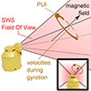 |
Fig. 3. Artistic rendition of the PLASTIC instrument (golden), its FOV is projected into 3D velocity space (red), and the trajectory of a PUI (turquoise) that gyrates around the magnetic field (black arrow). Parts of the PUIs example trajectory are outside the FOV. The probability of the particle to be measured is therefore lower than one. The inset at the bottom right provides the perspective, which looks from behind PLASTIC into its FOV. |
Thus, pitch-angle distributions need to be corrected for the influence of this effect, which we call ring coverage. In the following, the ring-coverage-based measurement probabilities are computed, and the pitch-angle distributions shown in this work are corrected through division by the ring coverage.
The ring-coverage-based measurement probabilities were computed per PHA event with the method described in detail by Keilbach (2023). The first step is to construct a ring that represents the trajectory and corresponds to the PHA event based on the current SW velocity, ϖSW, pitch angle, and the directions of the SW velocity and magnetic field vectors. Then, the intersections of the ring with the FOV boundaries are found (if existing). When no intersections exist, the ring is either fully inside or outside of the FOV, which leads to either full coverage (1) or no coverage (0). When boundaries exist, their angular distance is computed along the path that is inside the FOV. This distance divided by 2π is the ring-coverage-based measurement probability. The unlikely case that exactly one intersection with the FOV boundaries exists (the ring grazes the boundary) is treated as either full coverage or no coverage, respectively. In the case of more than two intersections with the boundaries, the corresponding points on the ring are separated into pairs, so that for each of these, the previous deliberations for two intersections apply. The sum of the resulting coverages of those pairs represents all points. Hence, the computational pattern for more than two intersections does not need extra description.
Figure 4 provides an illustration of the normalisation steps we applied. Panel b in Fig. 4 depicts an example of a raw PHA-derived pitch-angle distribution as a function of magnetic field azimuthal angle. Panel c shows the respective normalisation factors based on the frequency with which each magnetic field configuration was observed, and panel d gives the histogram after this normalisation was applied. In panel e the average ring coverage of the contributing particles is shown. Panels f and g show the result of the final normalisation for each half of the instrument: The influence of the events that contribute to panel d are weighted with the reciprocal of the ring-coverage-based measurement probability.
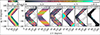 |
Fig. 4. Overview of instrumental resistive anode mapping (a) and normalisations (b to g) applied to the He+ data. All plots depict a quantity as a function of pitch angle (x-axis) and magnetic field azimuthal angle (y-axis). All identified He+ events are selected for which the conditions 0.9 < ϖinj, p < 1.1, π/16 < ϑB < π/16 and |λecl − 75|< 32 apply. Panel a depicts the average position channel measured by the PLASTIC resistive anode (average resistive anode channel, av. RA ch.). Panel b depicts He+ PHA data as counts per bin. Panel c depicts weights based on the number of instrumental weighting cycles during which the magnetic field angle was observed. These are applied in a first normalisation step. The result is shown in panel d as normalised counts per bin. Panel e depicts weights based on the coverage of a particle gyro orbit within the aperture of PLASTIC. Panels f and g depict the result of normalisation by these weights. The data from the φ < 0° and φ > 0° halves of SWS are separately depicted in panel f and panel g, respectively. |
In Sect. 5 we place the observations of this study into the context of Drews et al. (2015). To this end, we here provide a short overview of the differences in the respective data processing. (1) Drews et al. (2015) restricted the analysis to a 2D representation of the velocity space, whereas we considered the full 3D case. Since (2) Drews et al. (2015) restricted its analysis to cases for which the ring-coverage-based measurement probability is expected to be constant, this correction was not applied there. (3) Unlike in our study, the orbit-depending effect of the ISN velocity on the PUI velocity measure was not considered by Drews et al. (2015).
3. Definition of a injection-velocity-based PUI velocity measure
Table 1 provides a summary of the properties of PUI velocity measures, and Fig. 5e displays ϖSW spectra as a function of ecliptic longitude. Similar to the findings of Möbius et al. (2015), the velocity spectra are shifted as a function of ecliptic longitude. The reason for this systematic shift is that the velocity measure ϖSW of Eq. (1) does not account for the velocity from which the ISN originated. The ISN velocity causes a shift of the initial velocity of PUIs and due to orbital mechanics. Therein, the shift is a function of ecliptic longitude (Möbius et al. 2015; Lee et al. 2015; Taut et al. 2018). Möbius et al. (2015) corrected for the shift via a fit of a model curve to the cut-off of the orbital position-dependent ϖSW spectrum. This fit also yielded a then new way to determine the inflow direction of the LISM. Taut et al. (2018) increased the precision of the fit by taking various parameters into account, including vector information of the orientation of vSW and a model by Lee et al. (2015) of vISN.
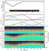 |
Fig. 5. ISN densities and velocities and the impact of the ISN velocities on relative velocity measures for PUIs over ecliptic longitude. All panels share a common x-axis and are a function of the ecliptic longitude. Panel a shows the fraction of primary ISN density, and panel b shows the radial and tangential components of the ISN velocity. Panel c shows spectra of ϖSW, inj, p, panel d shows spectra of ϖSW, inj, s and panel e shows spectra of ϖSW. All spectra are normalised to the respective maximum of the ecliptic longitude slices. The different symbols at the x-axes correspond to different ecliptic longitudes that correspond in heliospheric position to the markers in Fig. B.1: Focusing cone (yellow triangle), crescent (light pink square), and intermediate (magenta circle) position. |
However, in this study, the relative PUI velocity was computed from 3D vector information, and the corrections proposed by Möbius et al. (2015), Taut et al. (2018) therefore cannot be employed directly because they are ambiguous in direction. Therefore, a corrected ϖSW-like quantity is required that becomes one for freshly created PUIs. Since the velocity distance of a PUI to the transporting SW bulk vPUI − vSW is initially vSW − vISN, we propose that the velocity measuring quantity
 (2)
(2)
suits the purpose of uniquely identifying fresh PUIs with ϖSW, inj independent of ecliptic longitude. Since the computation of ϖSW, inj requires knowledge of vISN, computational means for computing the ISN trajectory and position-dependent velocity were implemented following Lee et al. (2015). Details are given in Appendix B. Table 1 compares the PUI velocity measure ϖSW, inj of our study to the two most commonly used velocity measures for PUIs.
Two distinct trajectories lead to any point in the heliosphere. Two different versions of ϖSW, inj are therefore necessary (ϖSW, inj, p and ϖSW, inj, s). Herein, p and s represent the primary and secondary trajectories, respectively. This distinction is determined based on the local ISN density under the assumption that the dominant process for reducing the ISN density is photoionisation. The trajectory with the higher remaining ISN density at the considered orbital position is labelled as primary, and the trajectory with the lower remaining ISN density is labelled as secondary. Figure 5a shows the fraction of primary trajectory density to the total ISN density as a function of ecliptic longitude over the orbit of STEREO-A. Since the primary trajectory ISNs makes up more than 0.8 of the total density everywhere except for ∼ ± 30° around the focusing cone (yellow triangle in Fig. 5), the secondary trajectory can be neglected outside the focusing cone region. Figure 5b shows the radial and tangential velocity components of the ISN velocity. Close to the focusing cone, the primary and secondary become similar, and at the symmetry point, they swap roles. Exactly at the focusing point, they are indistinguishable.
In the following, we take 75° as the ISN inflow direction. This represents a compromise of the different values derived in Taut et al. (2018) and Swaczyna et al. (2022). Panels c and d of Fig. 5 display ϖSW, inj spectra as a function of ecliptic longitude, analogously to the ϖSW spectra of Fig. 5e. Here, ϖSW, inj, p and ϖSW, inj, s are computed under the assumption that all observed PUIs followed the primary or the secondary component, respectively. Clearly, this assumption is unrealistic for the secondary trajectory outside the focusing cone region. Thus, Fig. 5d shows a strong position-dependent velocity shift for the secondary trajectory outside the focusing cone region that is amplified compared to the standard definition of ϖSW in Panel e. Because the contribution of particles following the secondary trajectory is expected to be negligible outside the focusing cone region, almost only PUIs of a primary ISN origin are found. The reference to the secondary injection point is therefore not suitable here.
In contrast, the ϖSW, inj, p spectra in Fig. 5c with their cut-off align well with the horizontal line at ϖSW, inj, p = 1. This illustrates that ϖSW, inj, p indeed works as a relative velocity measure, as intended. In particular, ϖSW, inj, p now allows a direct comparison of PUIs at different positions in the orbit of STEREO-A.
4. Traces of the torus of fresh PUIs
Based on 2D observations of STEREO-A/PLASTIC, Drews et al. (2015) found signatures that shifted in their observed direction as a function of the magnetic field direction. Drews et al. (2015) interpreted these observations as a torus of freshly injected PUIs (as illustrated here in Fig. 1) and referred to this structure simply as a torus. We follow this nomenclature in this study and emphasise that in this context, “torus” only refers to the torus signature of freshly injected PUIs. We extend the analysis from Drews et al. (2015) based on 3D observations and take our new injection-velocity-dependent ϖSW, inj into account.
For a direct comparison with Drews et al. (2015), we employ in this section the same 2D angle β (see Eq. (3) in Drews et al. 2015) of the relative PUI within the instrument aperture. When ϖSW of Eq. (1) is generalised to a vector quantity ϖSW by omission of the absolute in the numerator, then β can be interpreted as the polar angle of ϖSW in the (x, y)-plane, namely
 (3)
(3)
Our current study incorporated the ISN velocity during pick-up to increase the precision of the relative PUI velocity. Interestingly, modifications by the ISN pick-up velocity do not affect β. This is evident from an analysis of the fraction of ϖSW, inj, y/ϖSW, inj, x where the relation to the ISN velocity in the denominator cancels out, like
 (4)
(4)
However, since Drews et al. (2015) employed a ϖSW filter to limit the data for their (β, φB) histograms while we here filtered on ϖSW, inj, our updated versions of these histograms still depend on the full 3D observations and are expected to differ from the version of Drews et al. (2015). Figure 6 shows the angle β over the magnetic field azimuthal angle ϑB for different filters in ϖSW, inj. We observe an analogous torus feature as seen in Fig. 5 in Drews et al. (2015): The PUI observations peak at approximately 90°, and this peak shifts systematically with β to higher azimuthal angles. We interpret this as a verification of the torus signature reported in Drews et al. (2015).
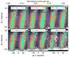 |
Fig. 6. 2D histograms of the angle β of Eq. (3) (y-axis) as a function of the magnetic field azimuthal angle (x-axis). Each histogram is accumulated from events from different intervals of ϖSW, inj, p. Each β-slice is normalised to its respective 99 percentile. |
 |
Fig. 7. 2D histograms of pitch angle (x-axis, from 0° to 180°; one tick equals 45°) and magnetic field azimuthal angle (y-axis, from −180° to 180°). The entirety of histograms is structured as a matrix. In each cell, the pitch-angle histograms for the primary ISN trajectory (P) are shown, and each row of histograms is filtered for a different ϖinj, P. The value range for a histogram is indicated on the left line. Each histogram is labelled P to indicate that all observations were treated as coming from the primary trajectory. Each column of histograms represents a different ecliptic longitude that is indicated on the bottom line. All histograms share the same global maximum after the normalisation steps displayed in Fig. 4 were applied. The dashed lines show the range of initial pitch angles to be expected at a given magnetic field azimuthal angle. In addition, a SW filter was applied (300 km/s ≤ vSW ≤ 450 km/s), and only data from the φ < 0° half of the instrument are shown here. |
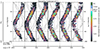 |
Fig. 8. 2D histograms of the pitch angle (x-axis, from 0° to 180°; one tick equals 45°) and the magnetic field azimuthal angle (y-axis, from −180° to 180°). The histograms are analogously structured and normalised as in Fig. C.1, except that only the row for 0.95 ≤ ϖinj, P ≤ 1.05 is shown, the observations are restricted to the region of the focusing cone, and each column refers to observations associated with a different SW velocity vSW. |
5. Pitch-angle distributions as a function of magnetic field orientation and ecliptic longitude
This section presents the He+ PUI observations as pitch-angle distributions as a function of the magnetic field azimuthal angle and sorted by the new PUI velocity measure. In the following, the magnetic field elevation angle is limited to in-ecliptic configurations of the magnetic field, and only the φ < 0° half of the SWS aperture is considered.
As an overview of the whole orbit of STEREO-A, Fig. 7 and Fig. C.1 display pitch-angle distributions as a function of magnetic field azimuthal angle and ϖSW, inj, P, grouped by the ecliptic longitude at which they were observed. The difference between Fig. 7 and Fig. C.1 is the normalisation of each histogram. In Fig. 7 all histograms share the same global normalisation, whereas in Fig. C.1 all histograms are normalised to their respective 99 percentile. Figure 7 clearly shows the expected enhancement of PUIs near the focusing cone at λecl = 75°. The dashed lines in each histogram indicate the expected position of a torus of freshly injected PUIs within the PLASTIC FOV, and most histograms show a clear enhancement at this expected torus position. In addition, our newly proposed PUI velocity measure ϖSW, inj, P shows a strong population of PUIs over all ecliptic longitudes in the range 0.85 ≤ ϖSW, inj, P ≤ 0.95. ϖSW, inj, P < 0.95 implies that these PUIs might not be freshly injected PUIs.
The individually normalised histograms in Fig. C.1 allow a more detailed comparison of the shapes of the respective distributions. Common to all histograms in Fig. C.1 are prominent features at pitch angles of ∼90°. These align with the regions in which the range of expected pitch angles of freshly created PUIs intersects the aperture (dashed lines). Especially for ϖSW, inj, P ∼ 1, this can therefore be interpreted as a strong signature of the torus of freshly created PUIs. However, even though the features clearly have a maximum where it would be expected for freshly created PUIs, the features are quite broad. Relative densities of > 0.25 are observed for magnetic field azimuthal orientations in 75° < |φB|< 135°. Close to φB = 0° and φB = ±180°, the relative density almost diminishes. This structure can at least partially be caused by the sensitivity range of the angular response function of the resistive anode of PLASTIC and the blind spot of the instrument in the centre (compare Fig. 4a). Hence, we cannot discount the possibility that additional anisotropic features are masked by the instrumental angular response and that the pitch-angle distributions therefore appear more isotropic. In the ϖSW, inj, P ∼ 1 row in Fig. C.1, however, the broadness of regions with relative densities > 0.75 increases and decreases with the ecliptic longitude.
Next, the differences between the histograms observed at the same ecliptic longitude but different ϖSW, inj, P (different rows in Fig. C.1) were considered. Under the assumption that transport effects are reflected in a ϖSW, inj, P smaller or larger than 1, primarily fresh PUIs are found at ϖSW, inj, P ∼ 1, and PUIs that have undergone transport and are thus modified have values higher than one if they have been accelerated and lower than one if have been decelerated 1. Under the assumption that only cooling and no acceleration occurred, the distance of ϖSW, inj, P to 1 can be interpreted as an age of PUIs with ϖSW, inj, P < 1. For older PUIs, the magnetic field configuration at the point of ionisation does not necessarily relate to the magnetic field configuration during observation of the particle. Hence, the range of initial pitch angles of PUIs as a function of the magnetic field azimuthal angle as it is plotted in the histograms is probably only a correct indicator for ϖSW, inj, P ∼ 1 and is more difficult to interpret in the other rows of Fig. 7 and Fig. C.1. Even without transport effects, the changing magnetic field conditions at each pick-up event would result in a broadening of the observed torus as a superposition of multiple tori oriented around different magnetic field directions.
Despite these arguments, the bottom panel of Fig. C.1 (slower PUIs) looks interestingly similar to the central panel. On the one hand, this could imply that the timescale of PUI modification by transport is not sufficient to create significant differences between the panels and that 0.85 < ϖSW, inj, P < 0.95 is close enough to one for most PUIs there to behave similarly to freshly injected PUIs. On the other hand, also the PUIs with ϖSW, inj, P ∼ 1 might already have experienced transport effects that did not obscure the torus signature completely, but already modified the pitch angle distribution in a similar manner as for the PUIs in 0.85 < ϖSW, inj, P < 0.95. Further, PUIs that were ionised close to but not directly at the spacecraft and under varying magnetic field conditions could also contribute to a broadening of the torus. However, we cannot rule out completely that the complex ageing effects and instrumental asymmetries together with insufficient statistics could obscure signatures of isotropic distributions (Keilbach 2023).
The data in the top panels of Fig. 7 and Fig. C.1 are noisier because fewer events contribute to the distributions. Despite this small statistic, it is interesting that the histograms of ϖinj, P > 1 show quite isotropic distributions, at least for all histograms outside the focusing cone. This tentatively indicates a possibly different transport behaviour of accelerated compared to cooled PUIs. We expect that this can be observationally verified or falsified with future studies with the instrumentation on board Solar Orbiter, IMAP, or Interstellar Probe, which build on the methods employed in our current study.
Figure C.2 displays pitch-angle distributions filtered not only by ϖSW, inj, P, which assumes that all PUIs followed the primary trajectory, but for comparison, also for ϖSW, inj, S, which assumes that all PUIs followed the secondary trajectory. At the focusing cone, based on Fig. 5, the velocities of the two ISN trajectories are expected to become similar and at the symmetry point swap their roles with regard to primary versus secondary trajectory. These expectations were tested here for ϖSW, inj, P and ϖSW, inj, S with regard to the similarity of the respective distributions at the focusing cone. Outside the focusing cone and crescent, the probability of encountering particles from the secondary trajectory is very low due to the r−2 dependence of ionisation. The filters for ϖSW, inj, P or ϖSW, inj, S each treat all PUIs as coming either from the primary or the secondary trajectory because the information on which of the two trajectories the PUI travelled prior to ionisation is lost. Therefore, distinguishing between these two filters is only meaningful close to the focusing cone, where both trajectories are relevant. The insignificance of the secondary ISN trajectory outside the focusing cone is convenient, since again there is no way found to distinguish the origin of the PUIs if the secondary trajectory were significant in density. Thus, at intermediate longitudes, it would be ambiguous but most important to decide whether to filter for ϖSW, inj, P or ϖSW, inj, S because there, the trajectories’ velocity vectors are most different from each other. Therefore, in all other figures in this study except for Fig. C.2, the secondary trajectory is disregarded because the corresponding histograms exhibit a misleading shift under the ϖSW, inj, S filter.
In Fig. C.2, each pair of the two pitch-angle distributions within 10° of the focusing cone coordinate (centre of Fig. C.2) is almost identical at all displayed ϖSW, inj, P and ϖSW, inj, S intervals. With more distance from the focusing cone centre, the ϖSW, inj, P and ϖSW, inj, S histograms become less similar to each other. At ecliptic longitudes not displayed, the difference becomes more distinct. That we find slightly different pitch-angle distributions with the small differences between ϖSW, inj, P or ϖSW, inj, S in the focusing cone region emphasises the importance of a correct selection of the velocity of the transporting frame to which the relative PUI velocity measure is related.
Figure 8 is restricted to the focusing cone and additionally filters by the SW speed vSW. For 250 km/s < vSW < 300 km/s, the maximum for |φB|> 0 tends to be slightly closer to 0° than the expected range of fresh PUIs. This also applies to the range of 300 km/s < vSW < 350 km/s. Then, with increasing vSW, a shift in the position of the maxima to higher pitch angles and |φB| is recognizable, which loosely correlates with vSW. In the last bin (500 km/s < vSW < 550 km/s), the statistical significance is low, and the distribution looks more isotropic than in the other vSW bins.
A definitive answer to whether there is a systematic relation between the maxima in the pitch-angle distributions and vSW requires more data. Since our new PUI velocity measure ϖinj, P makes PUI observation from the complete orbit of STEREO-A comparable, Fig. C.3 generalises Fig. 8 to the full orbit. In Fig. C.3, which includes more events than Fig. 8, the positions of the maxima do not shift systematically with vSW. However, the distributions appear narrower for low values of vSW, and the widths of the distributions appear to increase with vSW. This small effect could be caused by different transport and acceleration conditions in different SW regimes. For example, wave activity plays a stronger role for high SW velocities, whereas stream interaction regions that are acceleration sites for PUIs are more frequent at intermediate SW velocities. Whether these processes indeed influence the PUI distributions is beyond the scope of this paper and requires further investigation with future studies. Because Fig. 8 mixes different orbital locations and multiple orbits (even different solar cycle states, since the orbits between 2008 and 2015 are observed) as well as different states of instrumental ageing, the broadening might also be a result of a mix of instrumental and physical effects, however.
6. Conclusions
We reanalysed and recalibrated the STEREO-A PLASTIC He+ PUI data set. The recalibrated data set takes the full 3D PUI velocities into account and considers the unequal fraction of observable PUIs depending on how much of a gyro orbit falls into the FOV of PLASTIC. The resulting PUI distributions show a torus signature of freshly injected PUIs and thereby validate the results of Drews et al. (2015).
We defined a new version of a PUI velocity measure, ϖinj, which corrects for the projection of the ISN velocity. This allowed a direct comparison of PUIs over the complete orbit of STEREO for the first time. The concept can also be applied to refine the determination of the ISN inflow direction from Möbius et al. (2015), Taut et al. (2018).
We investigated pitch-angle distributions as a function of the magnetic field direction. Therein, the pitch-angle coverage is determined by the PLASTIC FOV and the magnetic field direction. This approach allowed us to observe unbiased partial pitch-angle distributions. The pitch-angle distributions were also sorted by our new ISN-velocity dependent ϖinj,. Within the focusing cone, we illustrated the symmetry between the primary and secondary trajectories that contribute to the PUI density. Over the complete orbit of STEREO, we observed torus signatures of freshly injected pick-up ions together with a probably already evolved but still similar population at lower ϖinj,. Within the instrumental limitations (e.g., ageing effects and potential contamination by protons, as discussed in detail by Keilbach 2023) of PLASTIC, these observations indicate the onset of transport effects. That a broadened torus signature is still visible for 0.85 < ϖSW, inj, P < 0.95 might imply that these PUIs were picked up upstream of the spacecraft and that transport effects have not yet had time to completely isotropise the distribution. For PLASTIC, the results we presented are limited by the available statistics and can currently therefore not yet provide estimates of the timescales of scattering, cooling, and heating processes. Future observations with better statistics, and in particular, at different radial distances, for example, with the Heavy Ion Sensor (HIS) as part of the Solar Wind Analyser (SWA; Owen et al. 2020) on Solar Orbiter and the Solar Wind and Pick-up Ion (SWAPI) on the Interstellar Mapping and Acceleration Probe (IMAP; Smith et al. 2024), can benefit from our position-independent PUI velocity measure and may provide the means for identifying the radial position of the maximum of He PUIs, which, as our results tentatively indicate, lie inside of 1 AU.
Consecutive acceleration and cooling processes that exactly cancel each other out, can also lead to ϖSW, inj, P ∼ 1.
Acknowledgments
This work was supported by the Deutsche Forschungsgemeinschaft (DFG) as WI 2139/12-1. We further thank the science teams of STEREO/PLASTIC and STEREO/IMPACT for providing the respective level 1 and level 2 data products.
References
- Acuña, M., Curtis, D., Scheifele, J., et al. 2008, Space Sci. Rev., 136, 203 [Google Scholar]
- Axford, W. I. 1972, in The Interaction of the Solar Wind With the Interstellar Medium, eds. C. P. Sonett, P. J. Coleman, & J. M. Wilcox, 308, 609 [Google Scholar]
- Biermann, L. 1957, Observatory, 77, 109 [Google Scholar]
- Drews, C., Berger, L., Wimmer-Schweingruber, R. F., et al. 2012, J. Geophys. Res., 117 [CrossRef] [Google Scholar]
- Drews, C., Berger, L., Taut, A., Peleikis, T., & Wimmer-Schweingruber, R. F. 2015, A&A, 575, A97 [NASA ADS] [CrossRef] [EDP Sciences] [Google Scholar]
- Galvin, A. B., Kistler, L. M., Popecki, M. A., et al. 2008, Space Sci. Rev., 136, 437 [Google Scholar]
- Gloeckler, G., & Geiss, J. 1998, Space Sci. Rev., 86, 127 [Google Scholar]
- Gloeckler, G., Geiss, J., Balsiger, H., et al. 1993, Science, 261, 70 [Google Scholar]
- Gloeckler, G., Schwadron, N. A., Fisk, L. A., & Geiss, J. 1995, Geophys. Res. Lett., 22, 2665 [Google Scholar]
- Gloeckler, G., Fisk, L. A., Geiss, J., Schwadron, N. A., & Zurbuchen, T. H. 2000, J. Geophys. Res., 105, 7459 [NASA ADS] [CrossRef] [Google Scholar]
- Gloeckler, G., Möbius, E., Geiss, J., et al. 2004, A&A, 426, 845 [NASA ADS] [CrossRef] [EDP Sciences] [Google Scholar]
- Isenberg, P. A. 1997, J. Geophys. Res., 102, 4719 [Google Scholar]
- Jian, L. K., Russell, C. T., Luhmann, J. G., et al. 2013, in Solar Wind 13, eds. G. P. Zank, J. Borovsky, R. Bruno, et al., AIP Conf. Ser., 1539, 191 [Google Scholar]
- Jian, L. K., Russell, C. T., Luhmann, J. G., & Galvin, A. B. 2018, ApJ, 855, 114 [Google Scholar]
- Jian, L. K., Luhmann, J. G., Russell, C. T., & Galvin, A. B. 2019, Sol. Phys., 294, 31 [NASA ADS] [CrossRef] [Google Scholar]
- Keilbach, D. 2023, Ph.D. Thesis [Google Scholar]
- Lee, M. A., Kucharek, H., Möbius, E., et al. 2012, ApJS, 198, 10 [NASA ADS] [CrossRef] [Google Scholar]
- Lee, M. A., Möbius, E., & Leonard, T. W. 2015, ApJS, 220, 23 [NASA ADS] [CrossRef] [Google Scholar]
- Luhmann, J. G., Curtis, D. W., Schroeder, P., et al. 2008, Space Sci. Rev., 136, 117 [Google Scholar]
- McComas, D. J., Schwadron, N. A., Crary, F. J., et al. 2004, J. Geophys. Res., 109, A02104 [NASA ADS] [CrossRef] [Google Scholar]
- McComas, D. J., Allegrini, F., Bochsler, P., et al. 2009, Sci, 326, 959 [Google Scholar]
- Möbius, E., Hovestadt, D., Klecker, B., et al. 1985, Nature, 318, 426 [Google Scholar]
- Möbius, E., Lee, M. A., & Drews, C. 2015, ApJ, 815, 20 [CrossRef] [Google Scholar]
- Moebius, E., Rucinski, D., Hovestadt, D., & Klecker, B. 1995, A&A, 304, 505 [Google Scholar]
- Němeček, Z., Ďurovcová, T., Šafránková, J., et al. 2020, ApJ, 889, 163 [CrossRef] [Google Scholar]
- Owen, C., Bruno, R., Livi, S., et al. 2020, A&A, 642, A16 [NASA ADS] [CrossRef] [EDP Sciences] [Google Scholar]
- Shestakova, L. 2015, Sol. Syst. Res., 49, 139 [Google Scholar]
- Smith, E., Kubota, S., Schwinger, M., & Scherrer, J. 2024, in 2024 IEEE Aerospace Conference, IEEE, 1 [Google Scholar]
- Sokół, J. M., Bzowski, M., Kubiak, M. A., & Möbius, E. 2016, MNRAS, 458, 3691 [CrossRef] [Google Scholar]
- Starkey, M. J., Fuselier, S. A., Desai, M. I., et al. 2021, ApJ, 913, 112 [NASA ADS] [CrossRef] [Google Scholar]
- Swaczyna, P., Schwadron, N. A., Möbius, E., et al. 2022, ApJ, 937, L32 [NASA ADS] [CrossRef] [Google Scholar]
- Tarnopolski, S., & Bzowski, M. 2009, A&A, 493, 207 [NASA ADS] [CrossRef] [EDP Sciences] [Google Scholar]
- Taut, A., Berger, L., Möbius, E., et al. 2018, A&A, 611, A61 [EDP Sciences] [Google Scholar]
- Vasyliunas, V. M., & Siscoe, G. L. 1976, J. Geophys. Res., 81, 1247 [NASA ADS] [CrossRef] [Google Scholar]
Appendix A: Averaging and integration of STEREO-A IMPACT MAG Magnetic field data
To match the cadence of PLASTIC, the vector 8 Hz data is averaged for each 5-minute measurement cycle of PLASTIC. This procedure synchronises the magnetic field measurements with the PUI PHA data. However, information is lost with regard to the detailed time evolution of the magnetic field and 5 minutes may not be an optimal timescale to obtain an average magnetic field relevant for the particles. At an absolute magnetic field of 5 nT, the gyration period of a He+ PUI is ∼52 s, at 4 nT, it is ∼65 s. Therefore, 1 minute could be a more meaningful time period. One could also interpret the 5-minute cadence of PLASTIC as an averaging over ∼5 gyro orbits. A detailed analysis of the impact of the averaging time period of the magnetic field is beyond the scope of this work. However, since the pitch angle is computed from the magnetic field orientation, a detailed look at the impact of the time window of averaging is an interesting topic for future studies and might increase the accuracy of this work’s approach.
The distribution of magnetic field angles resulting from 5-minute averaged MAG data is shown in Fig. A.1. This distribution is used as part of the normalisation process depicted in Fig. 4.
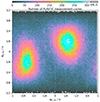 |
Fig. A.1. 2D histogram of the number of PLASTIC measurement cycles with magnetic field configurations selected by the azimuthal angle φB (x-axis) and the elevation angle ϑB (y-axis). |
Appendix B: Modelling of interstellar neutral trajectories
A central ingredient for a precise assessment of the history of a PUI is knowledge of the velocity vector of the ISN it originated from. This section focuses on its derivation.
B.1. Derivation of ISN velocity vectors and densities
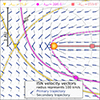 |
Fig. B.1. Illustration of the ISN velocities for different positions. The orbit of STEREO-A is indicated with a thin black line. Three pairs of example trajectories (primary with solid lines, and secondary with dashed lines) leading to the focusing cone (yellow), to the crescent (light pink), and an intermediate position (magenta) are shown. In addition, a grid of ISN velocities (in velocity space) is given for different positions in the inner heliosphere. The solid lines refer to the primary trajectory and the dashed lines to the secondary trajectory. |
To obtain the velocity vectors of ISN neutrals along the orbit of STEREO-A at ∼1 AU its direction at any point along its trajectory is required. The following derivation is similar to, for example, Lee et al. (2012). The trajectory of a He ISN is a Keplerian orbit (compare Sect. 1) and obeys the vis-viva equation
 (B.1)
(B.1)
Here, vISN is the ISN velocity, r the distance to the Sun, a the semimajor axis of the trajectory, and G the universal gravitational constant. For r → ∞ and therefore vISN → vISN, ∞ the equation simplifies to
 (B.2)
(B.2)
which for any a does not necessarily have a real solution. However, if the condition a < 0 for hyperbolas is incorporated, a may be replaced by −|a|, so that the negative sign vanishes on the right side. Then,
 (B.3)
(B.3)
is obtained, so a can be directly derived from the relative velocity between the heliosphere and the ISN, if the coordinate system is rotated such that the inflow direction coincides with the x-axis and the xy-plane is the plane in which the hyperbolic trajectory lies.
This is important for obtaining the semiminor axis b. While the absolute velocity at a solar distance of r is already fully described by a and vISN, ∞, the direction of the vector requires additionally the position at the orbit. For the hyperbolic trajectory in polar coordinates (r, φ) the parametrisation
 (B.4)
(B.4)
is employed. Herein,  is the eccentricity of the trajectory. The parametrisation requires that the focus point of the hyperbola is the gravitational centre. Thus, in the following, the Sun is the origin of the coordinate system. Also, the parametrisation requires that the periapsis coincides with the −x-direction. However, this is for most (but two) viewpoints at the orbit in contradiction to the earlier requirement that the x-direction is the direction of inflow. This can be solved by determining that the final trajectory is the result of a rotation around the z-axis of the parametrised trajectory. To determine the rotation angle, the initial angular coordinate of the parametrised trajectory is required. This angle, φ∞ is found through r → ∞ and is computed as
 (B.5)
(B.5)
Since the trajectory begins and ends at ±φ∞, two possible trajectories are found per coordinate in the heliosphere. From geometrical deliberations, it is found that the rotation angle of the trajectory is φR = ±φ∞ + λ0, where λ0 is the inflow direction. Since φ∞ is determined by ε and ε is determined by b and for b, a point at the orbit in ecliptic longitude λ and solar distance r needs to be chosen and the problem becomes too complicated to be solved analytically. Instead, such a required point for the trajectory to coincide with is determined by the input coordinates λ and r. The trajectory r(φ) is dependent on b through ε and its rotation to match the required input coordinates is dependent on b through φ∞. Hence, per orbit coordinate, b is found numerically and as an optimisation criterion, the minimum distance between the rotated trajectory and the required input point on the orbit is employed.
At this point, it is necessary to mention that by nature a Kepler trajectory is 2D. Here, it was implicitly assumed that the plane in which the trajectories are located is the in-ecliptic plane. As long as a cold model is assumed for the initial velocity of ISNs, this assumption holds true for all trajectories except for the trajectories passing through in the focusing cone or crescent region. In a hot model (not employed here), the direction of inflow would vary slightly from particle to particle, since then the initial velocity is drawn from a non-delta distribution. The model can represent an out-of-ecliptic velocity component by allowing an additional rotation of the trajectory around the medium inflow axis. Similar deliberations lead to a model of focusing cone and crescent region inflow trajectories: At those symmetry points, the entirety of trajectories is found by a rotation of the in-ecliptic trajectories around the symmetry axis. In conclusion, this leads to the following statements about the ISN velocity vectors in a cold model:
-
Per orbital coordinate (r, λ) two trajectories are found. In the focusing cone and the crescent, the rotation of the two leads to the entirety of trajectories. Everywhere else, exactly two trajectories are found.
-
At a fixed distance from the Sun, the absolute ISN velocity is constant, however its direction is decisive for the initial PUI velocity.
-
For the ISN velocity vector in the sense of this work’s model, only the radial (R) and tangential (T) components are relevant. Since in the focusing cone and the crescent region, the entirety of trajectories results from the rotation around the symmetry axis, the tangential and normal (N) components result from rotation of the original tangential component.
Since the ISN velocity components are readily obtained from the tangent of the computed trajectory, at this point two ISN velocity vectors per orbital coordinate are readily available. What remains, is a classification of the trajectories. For this, the probabilities of photoionisation and charge exchange ionisation of the ISNs are numerically integrated. This results in density and ionisation profiles along the trajectory. Therefore, the trajectory of higher density at the selected point along the spacecraft’s orbit is classified as primary and the other as secondary. The resulting ISN velocities are illustrated in Fig. B.1. Three example trajectories are shown that pass through the focusing cone, the crescent, and an intermediate position in STEREO-A’s orbit. The grid of velocity space representations show the local ISN velocities along the primary and secondary trajectories.
Appendix C: Additional pitch-angle histograms
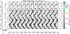 |
Fig. C.1. 2D histograms of pitch angle (x − axis, from 0° to 180° with one tick equalling 45°) and magnetic field azimuthal angle (y − axis, from −180° to 180°) in the same format as Fig 7 but here the histograms are normalised to their individual 99-percentile after the normalisation steps displayed in Fig. 4 were applied. |
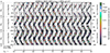 |
Fig. C.2. 2D histograms close to the focusing region of pitch angle (x − axis, from 0° to 180° with one tick equalling 45°) and magnetic field azimuthal angle (y − axis, from −180° to 180°) in the same format as Fig. C.1 with the exception, that pairs of histograms individually filtered by the velocity of the primary (P) or the secondary (S) ISN trajectory are shown for each combination of ϖinj, P/ ϖinj, S and ecliptic latitudes around the focusing cone. |
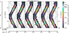 |
Fig. C.3. 2D histograms of pitch angle (x − axis, from 0° to 180° with one tick equalling 45°) and magnetic field azimuthal angle (y − axis, from −180° to 180°) in the same format as Fig. 8 but for full orbits. |
This section supplies three additional figures that are part of the discussion in Sect. 5. Figure C.1 shows pitch-angle distribution over the orbit of STEREO-A in the same format as Fig. 7 but each sub-histogram is normalised to its own maximum instead of the global maximum. Figure C.2 provides a detailed view of the focusing cone and compares the PUI velocity measure based on all particles following the primary trajectory ϖinj, P or the secondary trajectory ϖinj, S. Finally, Fig. C.3 shows the pitch-angle distributions organised by the SW speed over the full orbit of STEREO-A.
All Tables
All Figures
|
Fig. 1. three-dimensional (3D) visualisation of a freshly injected PUIs in velocity space in the SW frame of reference. The green arrows represent the SW bulk velocity, the black arrows show the local magnetic field, the blue arrows show the ISN velocity, and the amber ring shows the initial PUI VDF. The green hemisphere is a cut-out of the sphere of the entirety of velocities of fresh PUIs at the depicted setup of the SW velocity and ISN velocity. The different visualisations depict in total five different magnetic field configurations, and the other parameters are kept constant. |
| In the text | |
|
Fig. 2. Top left: Rendered side view of PLASTIC (cut in half). The entrance of the top hat of the cylindrical sensor is separated into two parts: The solar wind sector (SWS), and the wide-angle partition. Within the top hat, the electrostatic analyser is housed. In the lower parts of the instrument, the time-of-flight chamber and an solid state detector (SSD) are found. An example trajectory that enters the tophat is plotted in turquoise. Top right: Superimposed top-view cross-sections of PLASTIC. At the top, the entrance system is visible. At lower layers, the resistive anode and solid-state detectors are found. In purple we show the resistive anode channels, corresponding to the incident directions from the SWS aperture on the opposite side of the instrument. Bottom: Histograms of PLASTIC pulse-height analysis data from 2009. The left histogram shows the SSD energy channel as a function of the time-of-flight channel, wherein only events contribute that occur during energy-per-charge step 44. The dashed grey line shows the expected positions of He+ and He2+ for all energy-per-charge steps. The right histogram shows the energy-per-charge step as a function of time-of-flight channel. The dashed white line shows the expected average position of He+. The right histogram is normalised to individual maxima of time-of-flight slices. |
| In the text | |
|
Fig. 3. Artistic rendition of the PLASTIC instrument (golden), its FOV is projected into 3D velocity space (red), and the trajectory of a PUI (turquoise) that gyrates around the magnetic field (black arrow). Parts of the PUIs example trajectory are outside the FOV. The probability of the particle to be measured is therefore lower than one. The inset at the bottom right provides the perspective, which looks from behind PLASTIC into its FOV. |
| In the text | |
|
Fig. 4. Overview of instrumental resistive anode mapping (a) and normalisations (b to g) applied to the He+ data. All plots depict a quantity as a function of pitch angle (x-axis) and magnetic field azimuthal angle (y-axis). All identified He+ events are selected for which the conditions 0.9 < ϖinj, p < 1.1, π/16 < ϑB < π/16 and |λecl − 75|< 32 apply. Panel a depicts the average position channel measured by the PLASTIC resistive anode (average resistive anode channel, av. RA ch.). Panel b depicts He+ PHA data as counts per bin. Panel c depicts weights based on the number of instrumental weighting cycles during which the magnetic field angle was observed. These are applied in a first normalisation step. The result is shown in panel d as normalised counts per bin. Panel e depicts weights based on the coverage of a particle gyro orbit within the aperture of PLASTIC. Panels f and g depict the result of normalisation by these weights. The data from the φ < 0° and φ > 0° halves of SWS are separately depicted in panel f and panel g, respectively. |
| In the text | |
|
Fig. 5. ISN densities and velocities and the impact of the ISN velocities on relative velocity measures for PUIs over ecliptic longitude. All panels share a common x-axis and are a function of the ecliptic longitude. Panel a shows the fraction of primary ISN density, and panel b shows the radial and tangential components of the ISN velocity. Panel c shows spectra of ϖSW, inj, p, panel d shows spectra of ϖSW, inj, s and panel e shows spectra of ϖSW. All spectra are normalised to the respective maximum of the ecliptic longitude slices. The different symbols at the x-axes correspond to different ecliptic longitudes that correspond in heliospheric position to the markers in Fig. B.1: Focusing cone (yellow triangle), crescent (light pink square), and intermediate (magenta circle) position. |
| In the text | |
|
Fig. 6. 2D histograms of the angle β of Eq. (3) (y-axis) as a function of the magnetic field azimuthal angle (x-axis). Each histogram is accumulated from events from different intervals of ϖSW, inj, p. Each β-slice is normalised to its respective 99 percentile. |
| In the text | |
|
Fig. 7. 2D histograms of pitch angle (x-axis, from 0° to 180°; one tick equals 45°) and magnetic field azimuthal angle (y-axis, from −180° to 180°). The entirety of histograms is structured as a matrix. In each cell, the pitch-angle histograms for the primary ISN trajectory (P) are shown, and each row of histograms is filtered for a different ϖinj, P. The value range for a histogram is indicated on the left line. Each histogram is labelled P to indicate that all observations were treated as coming from the primary trajectory. Each column of histograms represents a different ecliptic longitude that is indicated on the bottom line. All histograms share the same global maximum after the normalisation steps displayed in Fig. 4 were applied. The dashed lines show the range of initial pitch angles to be expected at a given magnetic field azimuthal angle. In addition, a SW filter was applied (300 km/s ≤ vSW ≤ 450 km/s), and only data from the φ < 0° half of the instrument are shown here. |
| In the text | |
|
Fig. 8. 2D histograms of the pitch angle (x-axis, from 0° to 180°; one tick equals 45°) and the magnetic field azimuthal angle (y-axis, from −180° to 180°). The histograms are analogously structured and normalised as in Fig. C.1, except that only the row for 0.95 ≤ ϖinj, P ≤ 1.05 is shown, the observations are restricted to the region of the focusing cone, and each column refers to observations associated with a different SW velocity vSW. |
| In the text | |
|
Fig. A.1. 2D histogram of the number of PLASTIC measurement cycles with magnetic field configurations selected by the azimuthal angle φB (x-axis) and the elevation angle ϑB (y-axis). |
| In the text | |
|
Fig. B.1. Illustration of the ISN velocities for different positions. The orbit of STEREO-A is indicated with a thin black line. Three pairs of example trajectories (primary with solid lines, and secondary with dashed lines) leading to the focusing cone (yellow), to the crescent (light pink), and an intermediate position (magenta) are shown. In addition, a grid of ISN velocities (in velocity space) is given for different positions in the inner heliosphere. The solid lines refer to the primary trajectory and the dashed lines to the secondary trajectory. |
| In the text | |
|
Fig. C.1. 2D histograms of pitch angle (x − axis, from 0° to 180° with one tick equalling 45°) and magnetic field azimuthal angle (y − axis, from −180° to 180°) in the same format as Fig 7 but here the histograms are normalised to their individual 99-percentile after the normalisation steps displayed in Fig. 4 were applied. |
| In the text | |
|
Fig. C.2. 2D histograms close to the focusing region of pitch angle (x − axis, from 0° to 180° with one tick equalling 45°) and magnetic field azimuthal angle (y − axis, from −180° to 180°) in the same format as Fig. C.1 with the exception, that pairs of histograms individually filtered by the velocity of the primary (P) or the secondary (S) ISN trajectory are shown for each combination of ϖinj, P/ ϖinj, S and ecliptic latitudes around the focusing cone. |
| In the text | |
|
Fig. C.3. 2D histograms of pitch angle (x − axis, from 0° to 180° with one tick equalling 45°) and magnetic field azimuthal angle (y − axis, from −180° to 180°) in the same format as Fig. 8 but for full orbits. |
| In the text | |
Current usage metrics show cumulative count of Article Views (full-text article views including HTML views, PDF and ePub downloads, according to the available data) and Abstracts Views on Vision4Press platform.
Data correspond to usage on the plateform after 2015. The current usage metrics is available 48-96 hours after online publication and is updated daily on week days.
Initial download of the metrics may take a while.