| Issue |
A&A
Volume 588, April 2016
|
|
|---|---|---|
| Article Number | A12 | |
| Number of page(s) | 12 | |
| Section | The Sun | |
| DOI | https://doi.org/10.1051/0004-6361/201527603 | |
| Published online | 10 March 2016 | |
Anisotropy of the He+, C+, N+, O+, and Ne+ pickup ion velocity distribution functions
Institut für Experimentelle und Angewandte Physik (IEAP), Christian Albrechts-Universität zu Kiel, Leibnizstrasse 11, 24118 Kiel, Germany
e-mail: This email address is being protected from spambots. You need JavaScript enabled to view it.
Received: 20 October 2015
Accepted: 22 December 2015
Abstract
Context. Interstellar and inner-source pickup ions (PUIs) are produced by the ionization of neutral atoms that originate either outside or inside the heliosphere. Just after ionization, the singly charged ions are picked up by the magnetized solar wind plasma and develop strong anisotropic toroidal features in their velocity distribution functions (VDF). As the plasma parcel moves outwards with the solar wind, the pickup ion VDF gets more and more affected by resonant wave-particle interactions, changing heliospheric conditions, and plasma drifts, which lead to a gradual isotropization of the pickup ion VDF. Past investigations of the pickup ion torus distribution were limited to He+ pickup ions at 1 astronomical unit (AU).
Aims. The aim of this study is to quantify the state of anisotropy of the He+, C+, N+, O+, and Ne+ pickup ion VDF at 1 AU. Changes between the state of anisotropy between PUIs of different mass-per-charges can be used to estimate the significance of resonant wave-particle interactions for the isotropization of their VDF, and to investigate the numerous simplifications that are generally made for the description of the phase-space transport of PUIs.
Methods. Pulse height analysis data by the PLAsma and SupraThermal Ion Composition instrument (PLASTIC) on board the Solar Terrestrial RElations Observatory Ahead (STEREO A) is used to obtain velocity-spectra of He+, C+, N+, O+, and Ne+ relative to the solar wind, f(wsw). The wsw-spectra are sorted by two different configurations of the local magnetic field – one in which the torus distribution lies within the instrument’s aperture, φ⊥, and one in which the torus distribution lies exclusively outside the instrument’s field of view, φ∥. The ratio of the PUI spectra between φ⊥ and φ∥ is used to determine the degree of anisotropy of the PUI VDF.
Results. The data shows that the formation of a torus distribution at 1 AU is significantly more prominent for O+ (and N+) than for He+ (and Ne+). This cannot be explained by resonant wave-particle interactions as the sole mechanism for the isotropization of the PUI VDF. The anisotropy of the O+ VDF compared to He+ is highly fluctuating but consistently higher over an observation period of six years and therefore unlikely to be related to either specific heliospheric conditions or solar activity variations. To our surprise, we also found a clear signature of a C+ torus distribution at 1 AU very similar to the one of He+, although as an inner-source PUI, C+ should have a considerably different spectral and spatial injection pattern than interstellar PUIs.
Key words: Sun: heliosphere / solar wind / interplanetary medium
© ESO, 2016
 Open Access article, published by EDP Sciences, under the terms of the Creative Commons Attribution License (http://creativecommons.org/licenses/by/4.0),
which permits unrestricted use, distribution, and reproduction in any medium, provided the original work is properly cited.
Open Access article, published by EDP Sciences, under the terms of the Creative Commons Attribution License (http://creativecommons.org/licenses/by/4.0),
which permits unrestricted use, distribution, and reproduction in any medium, provided the original work is properly cited.
1. Context
The investigation of heliospheric pickup ions (PUIs) is of particular interest because of their role in the generation of and interaction with electromagnetic waves embedded inside the solar wind plasma (Cannon et al. 2014; Saul et al. 2009) and because of their diverse origins, which can range from sources that are only several solar radii away from the Sun (Geiss et al. 1995), the so-called inner-source of pickup ions, up to a distance of hundreds of astronomical units (au), the local interstellar medium (Moebius et al. 1985). The most important characteristics, unique to both interstellar and inner-source pickup ions, which also set them apart from other heliospheric ions are (1) their almost exclusive single charge state; (2) a highly non-thermal velocity distribution function (VDF) with a characteristic drop at wsw = | vion−vsw | /vsw ≈ 1 (e.g. Vasyliunas & Siscoe 1976); (3) a highly anisotropic VDF (Drews et al. 2013, 2015); and (4) a source population – although not directly observed – of neutral atoms somewhere between the observer and the Sun. The dimensionless quantity wsw is the velocity of the pickup ion, vion, relative to the solar wind velocity, vsw, in the frame of the solar wind, i.e. wsw is 1 if the pickup ion is twice as fast as the solar wind and 0 if vion = vsw.
After the initial phase of the pickup process, i.e. the neutral source population has just been ionized by either photo ionization, charge exchange with solar wind H+ or electron impact ionization, pickup ions are forced on gyro orbits that are perpendicular to the local magnetic field vector. Under the assumption that the source of neutral atoms was resting and that the pickup ions are co-moving with the solar wind after they have been ionized, the velocity of the resulting pickup ion population will range from 0 <w = vion/vsw< 2 in a resting and 0 <wsw< 1 in a solar wind frame of reference, respectively. Furthermore, the initial pickup ion VDF is expected to be highly anisotropic and distributed in the form of a torus at wsw = 1 (see Fig. 1, top panels). After a certain amount of time, however, the pickup ion VDF is expected to lose its initial torus shape as a result of the continuous influence of several mechanisms acting during the phase space transport between the PUI seed location and the observer. These processes are among others: pitch-angle scattering, which changes the PUI’s pitch-angle owing to resonant wave-particle interaction (Fig. 1, bottom right), acceleration and deceleration processes (Fig. 1, bottom left) and local disturbances of the solar magnetic field. For a detailed discussion on the influences of these processes on the formation and evolution of the He+ pickup ion torus distribution, see Drews et al. (2015).
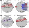 |
Fig. 1 Velocity space diagrams of a pickup ion torus distribution as a (vx,vy)-projection (top left panel) and in the vz = 0 km s-1 plane (top right) are shown for a magnetic configuration in which B is almost perpendicular. Here, vx, vy, and vz are the three vector components of vion, whereas vx is the velocity parallel to vsw. The bottom two panels show the torus distribution under the influence of pitch-angle scattering (right) and adiabatic cooling (left). To illustrate the torus character of the distribution, the (vx,vy)-plane is slightly tilted in this diagram. |
Processes that alter the initial form of the pickup ion VDF either act over time, e.g. adiabatic cooling and pitch-angle scattering, or along the trajectory of the pickup ion from its source location to the observer, e.g. solar magnetic field disturbances and magnetic drifts. Either way, pickup ions that are produced locally or at least in the vicinity of the observer, will generally be less influenced by these processes with the consequence that the initial torus form of the VDF is expected to be relatively intact during their observation. Interstellar pickup ions, although they are not exclusively produced locally at the observer, are therefore expected to show a clear torus or ring-beam feature at 1 au (Drews et al. 2013). Inner-source pickup ions on the other hand, which in the past have been attributed exclusively to a source close to the Sun (Geiss et al. 1995; Allegrini et al. 2005), are expected to show no, or at least a less pristine, feature of the torus at 1 au. Even during conditions of very low solar activity, in which the impact of pitch-angle scattering processes and local disturbances of the global solar magnetic field on the initial torus shape of the VDF are minimal, cooling processes (Fahr 2007; Chen et al. 2013) would still act on the VDF of inner-source pickup ions and therefore cause the initial torus distribution of these ions to be observed at significantly lower velocities, i.e. wsw < 0.5, compared to a locally produced pickup ion population (Drews et al. 2015), where it would be observed at wsw ≈ 1 (Fig. 1, lower left panel).
2. Aims
In this study, we present observations at 1 au of a torus signature of heavy pickup ions, i.e. C+, N+, O+, and Ne+. Our aim is to discuss these 1D observations of the pickup ions’ wsw-spectra in the light of our recent observation of the 2D velocity distribution function of He+ (Drews et al. 2015). The 2D observations of the He+ VDF and the corresponding 1D reduction (presented in this work) will serve as a guideline to interpret features of the pickup ion torus distribution of the heavier pickup ions, for which a 2D analysis of the VDF is very difficult owing to the limited counting statistics. In our study, we present a method to obtain the fraction of anisotropically distributed pickup ions to isotropically distributed ones by utilizing the observation of the pickup ion torus distribution at 1 AU in a solar wind frame of reference. Thereafter, we discuss the observed anisotropy of the pickup ions’ VDF in the light of resonant wave-particle interaction and cooling processes as the two main driver for the PUI phase space transport.
3. Data analysis
For this study we have used pickup ion data from the PLAsma and SupraThermal Ion Composition (PLASTIC) instrument (Galvin et al. 2008) and data of the local magnetic field vector from the In situ Measurements of PArticles and Coronal mass ejection Transients (IMPACT) instrument suite (Acuña et al. 2008), which are both mounted on board the Solar Terrestrial RElations Observatory Ahead (STEREO A) spacecraft. PLASTIC is a linear time-of-flight mass spectrometer, which by a measurement of an ion’s energy-per-charge, time-of-flight, and residual energy, determines the mass, mass-per-charge, and velocity of solar wind as well as suprathermal ions. PLASTIC is also capable of determining an ion’s velocity vector components vx, vy, and vz with x being defined as the connection between the spacecraft and the Sun, y being tangential to the spacecraft’s orbit and z being normal to x and y. An electrostatic deflection and position-sensitive detection system is used to derive an ion’s incident angle in azimuth, α, and polar direction, θ, respectively, which in turn are necessary to derive the pickup ion velocity in a solar wind frame of reference: 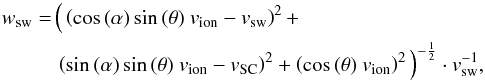 (1)where vion is the pickup ion’s total velocity, vsw the solar wind velocity and vSC the spacecraft velocity.
The method to extract He+ events from PLASTIC’s pulse-height analysis data has already been described in Drews et al. (2013) and is basically a matter of filtering the data by mass-per-charge and mass in order to separate He+ from other solar wind and suprathermal ions. The method to obtain wsw spectra for the heavy pickup ions with masses m> 8 amu/e is more complicated and will be explained in detail throughout this section.
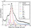 |
Fig. 2 Mass-per-charge spectrum of heavy pickup ions (Δm/q = 0.4 amu/e) observed by PLASTIC on board STEREO A. The data was accumulated for a period of 2400 days, beginning in March 2007, and C+ velocities of wsw,C+> 0.2 (open circles). A mass-per-charge model (dashed black line) was fitted to the data to obtain the absolute abundances of C+, N+, O+, Fe3+, Ne+, Mg+, and Fe2+ in terms of instrumental count rates. An exponential model was included to estimate and incorporate the influence of instrumental background to the mass-per-charge spectrum between 10 <m/q< 35 amu/e. |
The first step is to transform the time-of-flight and energy-per-charge information of the heavy pickup ions into a mass per charge. For that, a mass-per-charge algorithm was used that was already described in Drews et al. (2012). The resulting mass-per-charge spectrum for relative velocities of C+ of wsw> 0.2 are shown in Fig. 2 (open circles). Because of the relatively high mass and single charge state of heavy pickup ions, they are confined to a mass-per-charge range of m/q> 8 amu/e, which separates them clearly from the main solar wind constituents, e.g. H+, He2+, and O6+. To suppress the contribution of Fe2+ or Fe3+, a simple residual energy filter is applied to further separate the heavy pickup ions from the minor solar wind ions by their mass. Despite an internal post acceleration of 20 keV/e right before an ion’s time-of-flight measurement, the energy of most heavy pickup ions do not exceed PLASTIC’s energy threshold and these ions are therefore registered with their time of flight only. Owing to the rare nature of the heavy pickup ions it is therefore beneficial to include events with no residual energy measurement and, consequently, no mass information as well. For the most part Fe2+ and Fe3+ will deposit enough energy in PLASTIC’s solid state detector to surpass the energy threshold and to be clearly separated from the heavy pickup ions. However, the limited probability of triggering a residual energy measurement (despite an ion’s energy) (Galvin et al. 2008) is expected to generate some ion events that fall inside the mass-per-charge range of 7 <m/q< 35 and therefore contribute to the heavy pickup ion mass-per-charge spectra. These ions, which mainly consist of Fe2+ and Fe3+ must therefore be included in our mass-per-charge model for the heavy pickup ions.
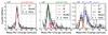 |
Fig. 3 Mass-per-charge spectra of heavy pickup ions obtained by PLASTIC on STEREO A for three different time periods in which either O+, C+, or Ne+ show a significantly increased abundance compared to other heavy pickup ions (panels from left to right respectively). These periods were used to obtain the necessary parameters for the mass-per-charge model (Eq. (2)) that is used to obtain the heavy pickup ion wsw-spectra. |
In the next step, we need to find a suitable mass-per-charge model for the individual heavy pickup ion species, i.e. C+, N+, O+, Ne+, and Mg+, as well as for the aforementioned ions, i.e. Fe2+ and Fe3+. The model, I(m/q), was adapted from Taut et al. (2015), where it was used to derive the composition of inner-source pickup ions with the charge and time-of-flight (CTOF) instrument on board the SOlar Heliospheric Observatory (SOHO; Hovestadt et al. 1995). Because of the very similar measurement principle of CTOF and PLASTIC, choosing the mass-per-charge model from Taut et al. (2015), which considers the asymmetry of the mass-per-charge model for an individual species, over a more simple, symmetric model (Drews et al. 2010) or a simple mass-per-charge filter (Drews et al. 2012), is most likely the best approach to deconvolve the contributions of individual species from the heavy pickup ion m/q-spectra. The model I(m/q) of an individual species, which is a combined Gaussian-κ-function, is given by ![Mathematical equation: \begin{equation} \label{eq:model} I(m/q) = A_0 \cdot \begin{cases} \ \exp{\left[-\frac{1}{2}\frac{\left(\frac{m}{q} - \mu\right)^2}{{\sigma_{\rm l}}^2}\right]} & \text{for} \hphantom{Hallo} \frac{m}{q}\ \leq \ \mu \\ \ \left[ 1+\frac{\left(\frac{m}{q}-\mu\right)^2}{\kappa{\sigma_{\rm r}}^2} \right]^{-\kappa} & \text{for} \hphantom{Hallo} \frac{m}{q}\ > \ \mu \end{cases} , \end{equation}](/articles/aa/full_html/2016/04/aa27603-15/aa27603-15-eq47.png) (2)with the peak amplitude A0, the peak position μ, the left and right peak widths σl and σr, and the asymmetry parameter κ.
(2)with the peak amplitude A0, the peak position μ, the left and right peak widths σl and σr, and the asymmetry parameter κ.
The relevant parameter for this study is A0 since it is proportional to the observed number of counts of a particular ion species. The parameters μ, σl, σr, and κ on the other hand are determined by the properties of the instrument and required to characterise the expected mass-per-charge models of ions entering the instrument. We describe the time-of-flight characteristics of the instrument using, specifically, the ion’s energy loss inside the foil. This energy loss is distributed asymmetrically around the most likely energy loss, which leads to m/q distributions that are also asymmetric. In our model, this is considered by the two different parameters σl and σr. Furthermore, the ion’s asymmetric energy loss distribution leads to time-of-flight distributions with pronounced tails, i.e. energy loss in the foil can only increase an ion’s time of flight. This is considered by the parameter κ. Of course, the aforementioned parameters for the m/q-model depend on the ion species, which further complicates a precise determination of I(m/q). Contrary to the analysis by Taut et al. (2015), who derived these parameters via a simulation of the time-of-flight characteristic of CTOF, we use a more direct approach via an in-flight observation, in which the m/q-spectra were significantly dominated by either C+, O+, or Ne+.
First of all, a time period between day of year (DoY) since 2007 between 127.3 < DoY < 127.5 was chosen to obtain a m/q-spectrum in which, almost exclusively, O+ from the Earth’s magnetosphere was observed with PLASTIC on STEREO A (Fig. 3, left panel). This period was used to obtain the parameters for the m/q-model of O+ via a fit of Eq. (2) to the data between 14 < m/q< 18. The second period between 1936 < DoY < 1937 (Fig. 3, centre panel) was used to derive the parameters of C+ for which the superposition of I(m/q) for C+, N+, and O+ was fitted to the data between 10 < m/q < 16. For the fit, the parameters of O+ were fixed to values obtained from the first time period, while the parameters of N+ were set to be identical to the ones from C+. Because the fit did not yield a significant difference for the parameters of C+ and O+, the resulting parameter set for C+ and N+ is assumed to be identical to O+. The last period was obtained during times in which the ecliptic longitude, λ, of STEREO was in between 65° < λ < 85° and the velocity of Ne+ between 0.9 <wsw < 1.1, i.e. time periods in which the abundance of Ne+ should be significantly increased as a result of the focusing cone (Drews et al. 2010). In this period, a superposition of I(m/q) for O+, Fe3+, and Ne+ was fitted to the data set between 15 < m/q < 24. Again, the parameters of I(m/q) for O+ were held constant, while the parameters for Fe3+ were assumed to be identical to the ones from O+, because no significant deviation between O+ and Fe3+ could be found. The obtained parameter set for Ne+ were then also used for Fe2+ and Mg+, which could not be obtained individually owing to their very low abundance.
As a final step, we also added a background model to account for random time-of-flight coincidences (Taut et al. 2015). The background model B(m/q) can be described with a single κ-distribution  (3)where μg and κg were found to be 5.4 and −1.31 via a fit to the long-term data.
Parameters of the mass-per-charge model, I(m/q), for the individual heavy pickup ion species
The final set of parameters of σl, σr, and κ for C+, N+, O+, Fe3+, Ne+, Fe2+, and Mg+ are summarised in Table 3. The peak heights A0 of the individual ions were then determined by a fit of Eq. (4) (8 degrees of freedom, one for each ion and the background model) to the long-term data. The final m/q model, used to obtain the individual count rates of the heavy pickup ions, is then given by  (4)and is shown as the dashed line in Fig. 2.
To obtain a wsw spectrum from a fit of the individual peak heights via Eq. (2), the long-term data between 7 <m/q< 35 is filtered for each ion included in our model by the respective velocity window wsw ± Δwsw of that ion (Δwsw = 0.05). The determined peak heights, A0, which are derived by a simultaneous fit of all ions included in our model F(m/q) to the filtered data, are then used to derive the amplitude of the model I(m/q) of that individual ion. The model I(m/q) then gives us the number of counts observed for that particular ion at a given velocity wsw ± Δwsw (Eq. (1)). This process is repeated for each species and velocity step wsw, which yields the number of counts for every ion as a function of that ion’s relative velocity window wsw ± Δwsw. The results for a long-term accumulation over 2400 days are shown in Fig. 4 for He+, C+, N+, O+, and Ne+. The wsw-spectra were corrected for the orbital velocity of the STEREO spacecraft and instrumental phase space coverage, i.e. data was only accumulated during times in which vsw < 450 km s-1 to assure that each ion is covered by the instrument up to at least wsw = 1.2. The reader should also keep in mind, that Fig. 4 only shows the measured counts by PLASTIC as a function of wsw and is therefore not proportional to a phase-space density, as is commonly used for the velocity spectra of pickup ion throughout the literature.
3.1. A remark on the ambiguity of F(m/q)
We note that a systematic deviation between F(m/q) (Eq. (4)) and the unknown, “real” m/q distribution of the heavy pickup ions will not only bias, but also systematically change values obtained for the individual peak heights A0 of C+, N+, O+, Fe3+, Ne+, Mg+, and Fe2+. Although we were able to determine the parameters of I(m/q) (Eq. (2)) for C+, O+, and Ne+ via direct observations, i.e. we used as few assumptions as possible, the time-of-flight characteristics of the instrument are influenced by instrumental aging effects which, in turn, can cause the parameters of I(m/q) to change over time. The fact that we have not found a noticeable degradation of the quality of the fit to the data during different time periods, does not necessarily mean that aging effects are insignificant but, rather, that changes in the parameters of I(m/q) are subtle and difficult to quantify.
Furthermore, the parameters of I(m/q) for N+, Fe3+, Mg+, and Fe2+ were not derived via a fit. The limited mass-per-charge resolution of the instrument and the low abundance of these ions made it impossible to derive individual parameter sets for these species. We therefore chose to use the parameter set of C+ and O+ also for N+ and Fe3+, while Mg+ and Fe2+ share the same parameter set with Ne+. This will of course introduce a systematic error to the values obtained for A0 of N+, Fe3+, Mg+, and Fe2+. Our results for these ions should therefore be treated with caution.
In addition, the underlying algorithm to determine the mass-per-charge from an event’s time-of-flight and energy-per-charge information was calibrated for the mass-per-charge range between 8 < m/q < 22 (Drews et al. 2010). However, for ions in the range of m/q > 16, the parameter μ had to be “fine-tuned” to obtain the optimal fit result to the long-term data (see Table 3), i.e. μ was slightly decreased with respect to the nominal mass-per-charge of these ions.
And finally, our selection of ions that are included in F(m/q) (Eq. (4)), i.e. C+, N+, O+, Fe3+, Ne+, Mg+, and Fe2+, may introduce a bias to our analysis. In the past, Geiss et al. (1995) and Gloeckler and Geiss (2001) have reported on an observation of the isotope 22Ne+ and several molecules, CH+, OH+, and H2O+ with Ulysses SWICS, while Taut et al. (2015) has reported on the observation of Mg2+, Al+, and Si+ with CTOF. Not including these ions in our model F(m/q) will especially affect our result for ions with m/q > 16 amu/e, since they might also contain contributions of the aforementioned species that were not included in our selection. However, we also note that this kinds of contribution are expected to be minimal with the exception of Si+. We did not explicitly add Si+ to our model because of the mass-per-charge algorithm not being able to distinguish between Mg+ and Si+. Results for Mg+ should therefore be seen as the combined mix of both Si+ and Mg+.
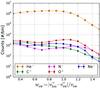 |
Fig. 4 Pickup ion velocity spectra, f(w), of He+, C+, O+, and Ne+ as a function of wsw = | vion−vsw | /vsw. Due to systematic and statistical uncertainties of the underlying mass-per-charge model, a reliable prediction for the velocity spectra of Fe3+, Mg+, and Fe2+ (and partially N+) is hardly possible. The spectra were corrected for the orbital velocity of the spacecraft and instrumental phase space coverage, but no instrumental response function to correct for the varying detection efficiency was applied (see text for details). |
4. Method
As described in Drews et al. (2015), the observation of a torus or ring-beam signature of He+ pickup ions is confined to specific configurations of the local magnetic field vector. These configurations depend mainly on the angular acceptance of the observing instrument. For instance, the solar wind section of the PLASTIC instrument provides an angular acceptance in the ecliptic plane, i.e. vz = 0 km s-1, of − 22.5° < α < 22.5°, and out of the ecliptic plane of − 20°< θ < 20°. For clarification, an ion entering the instrument at the angles α = 0° and θ = 0°, would stream radially away from the Sun. Because the pickup ion torus distribution changes its inclination as a function of the local magnetic field direction (Fig. 1), PLASTIC is only capable of observing the pickup ion torus for magnetic configurations in which the direction of the local magnetic field vector, defined by φB and θB, points away from the entrance system of the instrument by at least 90°. The specific magnetic configuration for which PLASTIC is capable of observing the torus distribution of pickup ions, φ⊥, or not, φ∥, is illustrated in Fig. 5 and summarised in Table 2.
Definition of the magnetic configurations φ⊥ and φ∥ in which PLASTIC can and cannot observe the pickup ion torus distribution respectively.
To analyse the torus distribution of the heavy pickup ions, we quantify the increase in flux induced by the initial torus distribution of He+, N+, C+, O+, and Ne+ as a function of wsw. As already pointed out, the low statistics available for the heavy pickup ions impedes an analysis of the 2D VDF as we have done for He+. However, with the work done on He+ (Drews et al. 2013, 2015), we understand very well how 2D signatures of the pickup ion torus affect and transform into a 1D representation of the VDF. First of all, we need to derive the long-term wsw-spectra for the two magnetic configurations illustrated in Fig. 5. This is done is analogy to the long-term wsw-spectra presented in Fig. 4, i.e. we derive the total pickup ion counts as a function of wsw via a fit of Eq. (4) to the m/q spectra obtained during periods in which the local magnetic field vector corresponds to either φ⊥ or φ∥. Furthermore, we only use periods in which vsw < 450 km s-1 to make sure that all pickup ions with m/q < 20 amu/e can be detected with a velocity of up to wsw = 1.2. Finally, the obtained counts as function of wsw for each pickup ion are transformed into a count rate as a function of wsw. This makes the intensity of the final spectra obtained for φ⊥ and φ∥ comparable to each other, i.e. the ratio f(wsw)⊥/f(wsw)∥ would be constant as a function of wsw if there is no difference in the shape of f(wsw)⊥ and f(wsw)∥.
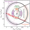 |
Fig. 5 Illustration of the two different magnetic configurations (inner circle) and corresponding pickup ion torus configuration (outer circle) used throughout this work. For the configuration φ⊥, i.e. the magnetic field vector B points in the direction of the orange shaded area within the inner circle, the pickup ion torus is located in a region of velocity space where it can be detected by the instrument (outer orange shaded ring). For the configuration φ∥, the torus lies exclusively outside the instrument’s aperture and cannot be detected (outer violet shaded ring). The torus distribution, shown in this diagram (red line), corresponds to the magnetic field vector drawn in red. |
Figure 6 shows the ratio  (5)for He+, C+, N+, O+, and Ne+, from left to right respectively. As previously described, the ratio R(wsw) is a measure for the fraction of pickup ions that are torus-distributed with respect to ions that are distributed isotropically, i.e. R(wsw) > 1 means that we observe more ions that are torus-distributed than ions that are distributed isotropically. For instance, at wsw ≈ 1.0, PLASTIC observes twice as many torus-distributed He+ ions (configuration φ⊥) compared to He+ ions that are distributed isotropically (configuration φ∥). However, PLASTIC cannot measure pickup ions below wsw ≲ 0.2 and is therefore not capable of covering the complete pickup ion torus distribution (see Fig. 5). Consequently, the ratio R(wsw) is not the same as the absolute increase in flux resulting from a torus feature, but it is proportional to it. It is especially important to note that f(wsw)⊥ and f(wsw)∥ were obtained for each ion under similar conditions, i.e. a similar solar wind velocity, density, temperature, and the same magnetic configuration, so that the ratio R(wsw) is at least comparable between He+, C+, N+, O+, and Ne+. Thus we can quantify the flux increase as a function of wsw resulting from a torus or anisotropic distribution of one ion in relation to another and, therefore, determine the relative impact of pitch-angle scattering or other phase-space-altering processes on different pickup ion species.
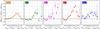 |
Fig. 6 The ratio, R(wsw) (Eq. (5)), of the pickup ion flux as a function of wsw between magnetic configurations φ⊥ and φ∥ for He+, C+, N+, O+, and Ne+ (panels from left to right). The data was collected between March 2007 and December 2013 during periods in which the solar wind velocity was below 450 km s-1. As illustrated in Fig. 5, the magnetic configurations φ⊥ and φ∥ correspond to configurations in which the pickup ion torus lies inside and outside the instrument’s aperture respectively. The ratio f(w)⊥/f(w)∥ is therefore an indicator of the relative flux increase induced by the pickup ion torus distribution or, in more general terms, an indicator for the anisotropy of the pickup ion VDF. |
5. Discussion
It was shown by an analysis of the 2D velocity distribution function of He+ (Drews et al. 2013, 2015) that an increase in R(wsw), i.e. an increase in the pickup ion flux during perpendicular configurations of the local magnetic field with respect to parallel ones, is linked to the observation of a torus-distributed pickup ion VDF. The formation of a torus distribution is a natural consequence of the interplay between the solar magnetic field and a resting neutral atom population that has just been ionized (Fig. 1). For He+ (left panel, Fig. 6) we see a significant increase of R(wsw) centred around wsw ≈ 1.1. This corresponds to our analysis of the He+ 2D VDF (Drews et al. 2015) and generally is expected for pickup ions of interstellar origin. At wsw ≈ 1.0, pickup ions have not yet suffered from adiabatic cooling and, therefore, must have been produced close to the observer. Pickup ions that were produced close to the observer had less time to be influenced by pitch-angle scattering or other phase-space-altering processes and therefore should show the highest ratio of torus or anisotropically distributed PUIs compared to isotropic PUIs. In the case of He+ at wsw ≈ 1.1, the maximum flux increase R(wsw) is 2.0, which means that within a short time frame after the ionization of interstellar neutral He at 1 au, ~60% of the newborn He+ pickup ions will be scattered out of their initial torus distribution (see Eq. (7)). By way of analogy, the ratio R(w) decreases with decreasing values of wsw until it reaches ~1 for the lowest wsw, i.e. almost all He+ pickup ions observed at 1 au are distributed isotropically in phase space if they were produced close enough to the Sun. A behaviour similar to He+ is also observed for Ne+, which is also predominantly of interstellar origin (5th panel, Fig. 6).
For O+, we observe a maximum of R(wsw) that is shifted towards higher wsw’s with a peak intensity of ~3. The shift is a result of oxygen having a lower first ionization potential (FIP) of 13.6V than either He or Ne (24.6V and 21.6V respectively). A lower FIP means that oxygen is less likely to reach the down-wind side of the Sun compared to He and Ne before being ionized. Therefore, the main production of interstellar O+ happens in the up-wind region where the higher relative velocity between the solar wind and the interstellar neutrals causes O+ to be produced with a higher initial velocity. N+ has a FIP of 14.5V and, consequently, shows a distribution of R(wsw) comparable to O+, despite the large uncertainties of our mass-per-charge model for N+.
Remarkably, C+ also shows a significant increase of R(wsw) at wsw ≈ 1.1, which is quite similar to what we observe for He+ and Ne+ while, at lower wsw, C+ seems to stream predominantly parallel to the ambient magnetic field. We know from several studies (Geiss et al. 1995; Schwadron et al. 2000, e.g.) that C+ pickup ions are unlikely to be of interstellar origin and, in fact, originate from inside our solar system.
Our observation of the PUI VDF isotropy at 1 AU shown in Fig. 6 are the result of two main aspects:
-
1.
Where and at what velocities these particles are injected.
-
2.
The evolution, i.e. phase-space transport, of PUIs after their injection.
-
(1)
Different PUI species have different injection patterns, i.e. PUI production rates depend on the position and species of their source atoms. The main driver for the spatial distribution of the production of interstellar PUIs are ionisation processes. These processes are species-dependent and determine the local production by the integrated depletion of interstellar atoms along their trajectories and the local ionisation rate of neutrals. The velocity distribution of interstellar neutrals is determined by their temperature in the local interstellar medium and is further altered by the gravitational force of the Sun. Although the detailed nature of the inner source is not sufficiently well understood to make meaningful predictions about the injection of these PUIs, it is certain that the properties of the inner source are different from the interstellar source.
-
(2)
The phase-space transport of PUIs after their injection depends on processes that act along the trajectories of the PUIs. For example, one of these processes that is believed to play a major role in the isotropisation of PUIs is resonant wave-particle interaction, which strongly depends on mass per charge and thus on the species. Another process which is generally believed to play a major role is adiabatic cooling caused by an adiabatic expansion of the PUIs. This cooling is often used to deduce the point of ionization from the observed PUI velocity. In the following two sections, we discuss our observations of R(wsw) in the light of these two aspects.
5.1. The Importance of resonant wave-particle interaction for PUI pitch-angle isotropization
From the observations shown in Fig. 6, we can directly infer the degree of anisotropy of the pickup ion VDF. Because R(wsw) is a measure for the flux increase that is due to the formation of a torus or, rather, an anisotropically distributed VDF as a function of wsw, we can easily obtain the fraction of pickup ions that have already been scattered out of their initial anisotropic state. For instance, a ratio of R(wsw) = 3 implies that only ~50% of the observed pickup ions are distributed isotropically in phase space. However, this is based on the assumption that (1) the anisotropic state of the pickup ion VDF is solely caused by the initial pickup ion torus distribution, and that the torus distribution behaves as described in Drews et al. (2015). This means that (2) the inclination of the torus systematically changes with the orientation of B; (3) it does not change in intensity as a function of its orientation and especially that (4) a torus distribution is a common feature neither confined to special heliospheric conditions nor individual pickup ion species.
Based on our studies of the 2D He+ velocity distribution function in Drews et al. (2013, 2015) and this work, we can say with certainty that assumptions (2) and (4) are universally valid. Assumption (3), i.e. the torus distribution does not change in intensity as a function of the orientation of B, is only partially true, as is evidenced by an observation of a partially increasing degree of isotropy of the He+ VDF during local IMF configuration close to the Parker field configuration. Here, transport effects can cause the torus distribution to spread in velocity space, as was shown in Drews et al. (2015). However, intensity changes in the torus signature owing to this effect are subtle and unlikely to affect the torus-induced flux increase significantly. Assumption (1), i.e. the anisotropy state of the VDF is solely caused by the occurrence of a torus signature, is difficult to prove. There have been several studies that claim that the pickup ion VDF has a bi-hemispherical structure, basically a different form of anisotropy, which is produced by a rapid but incomplete isotropization of the VDF (e.g. Isenberg 1997). Despite the fact that the assumption of a bi-hemisperical pickup ion VDF has been used to explain flux increases during perpendicular IMF configuration and to obtain parameters of either either the mean free path and adiabatic cooling index of He+ pickup ions (e.g. Isenberg 1997; Saul et al. 2007; Chen et al. 2013), there is no direct observational evidence for the pickup ion VDF having a bihemispherical structure. In fact, flux increases during perpendicular IMF configuration have been shown to be produced by the pickup ion torus distribution instead (Drews et al. 2013).
In the following, we apply the commonly made simplifying assumption for the PUI phase space transport that PUIs behave like an ideal gas and expand adiabatically. For this, we will follow the approach by Vasyliunas & Siscoe (1976), who applied the concept of adiabatic cooling for an isotropic pickup VDF. We note that the observations of a pickup ion torus distribution presented in (Drews et al. 2013, 2015) and this study, i.e. the PUI VDF is clearly not isotropic, is strong evidence for the fact that PUIs do not expand in a purely adiabatically way. However, we will pursue this approach to illustrate some of the misconceptions of the PUI phase space transport that are often implicit in the literature. With the assumption of a cooling process (Parker 1965; Isenberg 1987) produced via either an adiabatic (γ = 1.5) or magnetic (γ = 1.0) cooling mechanism, we can estimate the distance from the Sun where the PUIs were ionized as a function of wsw, i.e.,  (6)Of course, in reality there is also no universal cooling index, γ, for either adiabatic or magnetic cooling. Instead, the cooling index γ depends on several factors and is expected to fluctuate considerably as a function of time (Chen et al. 2013). With our results shown in Fig. 6, we can obtain the number of pickup ions that have been scattered out of their initial torus distribution as a function of wsw, and with Eq. (6) also as a function of the radial distance between the pickup ion’s location of injection, r, and the observer, r0. The fraction of isotropically distributed particles, ψ, of the VDF as a function of r0−r can be obtained using Eq. (6)
 ![Mathematical equation: \begin{eqnarray} \label{eq:rr} \psi(r_0-r) = 1 - \left[\left(R(w_{\rm sw})-1\right)/R(w_{\rm sw})\cdot \eta(w_{\rm sw})\right]. \end{eqnarray}](/articles/aa/full_html/2016/04/aa27603-15/aa27603-15-eq120.png) (7)
(7)
Here, the parameter η(wsw) accounts for the different phase-space coverage of the PUI isotropic shell and torus distribution caused by PLASTIC’s limited field of view. In Fig. 7, the result for ψ(r0−r) of He+ and O+ are presented for a cooling index of γ = 3/2. Results for C+, N+, and Ne+ are not shown owing to the large uncertainties (Fig. 6) that are due to strong inner-source contributions or substantial statistical fluctuations of the count rate. It also noteworthy that at small wsw and correspondingly long travel distances (Eq. (6)), contributions of inner-source He+ and O+ result in an anisotropy that is produced by a predominant streaming along the local magnetic field, as was already observed in Drews et al. (2015). Corresponding points in Fig. 7 are plotted as solid squares.
Mean travel distance, Λ, after which 80% of He+ and O+ pickup ions are distributed isotropically in velocity space for three different cooling indices, γ.
With the results from Fig. 7, we can obtain the average travel distance after which 80% of He+ and O+ pickup ions have undergone enough interactions to be scattered out of their initial anisotropic torus distribution. Here we assumed that the minimal travel distance (~0.05 au) is situated at the maximum of R(wsw) for each ion (Fig. 6), i.e. for He+ at wsw = 1.1 and for O+ at wsw = 1.2. This path length, Λ, is summarised for O+ and He+ in Table 3 for three different values of the cooling index γ. The cooling indices were chosen to lie in the range of the observed fluctuations of γ found in Chen et al. (2013). Cooling indices close to unity generally correspond to deceleration mechanisms, which are connected to magnetic cooling (Fahr 2007), while indices close to 1.5 correspond to an adiabatic pickup ion deceleration (Parker 1965; Isenberg 1987). On global scales, He+ shows path lengths, Λ, that lie universally below 0.5 AU, while the isotropization of O+ happens on larger scales than helium, i.e. the isotropization of the He+ VDF is significantly faster than for O+.
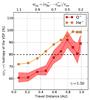 |
Fig. 7 The fraction of isotropically distributed pickup ions as a function of their travel distance from their production location up to 1 AU. The travel distance was calculated based on the assumption of an ideal adiabatic expansion with a cooling index of 3/2. Circular and square markers respectively denote whether the anisotropy is produced by pickup ions that stream in predominately perpendicular way or parallel to the local magnetic field. |
Under the assumption of a typical interplanetary magnetic power spectrum at 1 au, which scales as f− 5/3 (e.g. Bruno & Carbone 2013), the higher mass per charge and consequent lower gyration frequency of O+ compared to He+ means that O+ is in resonance with ranges of the fluctuation spectrum that carry significantly more power than for He+ (more by a factor of ~10). In other words, if the main mechanism responsible for the isotropization of the pickup ion VDF were resonant wave-particle interactions, O+ would show a significantly less anisotropic VDF than He+, as shown in this work (Fig. 7). Furthermore, a systematic trend of the VDF isotropy increasing with increasing pickup ion mass-per-charges (He→C→N→O→ Ne) should be visible, but is clearly not observed (Fig. 6). This is a critical finding, which probably has implications beyond the transport of PUIs.
At this point we also emphasise that the description of the pickup ion phase-transport processes used to determine values for Λ (Table 3) is strongly idealised (see Eqs. (6) and (7)). If we consider Eq. (7), the PUI VDF would show no isotropy during the initial part of the injection and combined with Fig. 7 this implies that the initial isotropization of the PUI VDF on scales of 0.05 AU would not only be extremely fast, but also continuous at a much slower pace after that. In reality, the isotropization of the PUI VDF should happen more gradually because it clearly depends on the number of pitch-angle scattering processes the PUIs have undergone and, therefore, the PUI’s lifetime. The derived distributions of the O+ and He+ anisotropy presented in Fig. 7 already indicate that the adiabatic expansion of PUI is probably too simple to describe the PUI phase-space transport.
Of note, the values of Λ presented in Table 3 were obtained for a total observation period of ~6 years. The mean travel distance after which 80% of He+ and O+ are distributed isotropically in velocity space, is expected to fluctuate because of the dependence on the global and local conditions of the interplanetary magnetic field. Several other factors, like the influence of acceleration regions, varying ionization rates, and general variations of the solar activity are expected to influence the results for ΛHe+ and ΛO+ as well. In Fig. 8 the anisotropy at r0 of the He+ and O+ VDF, ψ(r0), is shown as a function of time over the observation period between 2007 and 2013. While the significant difference of ψ(r0) between He+ and O+ remain even as a function of time, strong fluctuations become evident which, in the case of He+, are not caused by counting statistics, but rather by variations of the aforementioned global and local conditions of the heliosphere.
 |
Fig. 8 The fraction of isotropically distributed He+ (yellow) and O+ (red) pickup ions at r0 as a function of time (He: Δt = 30 d, O: Δt = 100 d). The solid and dashed lines denote the average and standard deviation of ψ(r0), respectively. |
In this context, it is also necessary to discuss the potential impact of a modulation of the PUI velocity spectra for the observed fluctuation of ψ(r0) shown in Fig. 8. This might be especially useful to raise the awareness about the limitations of our analysis and, therefore, to estimate the significance of the anisotropy parameter ψ(r0) presented in this study. In general, fluctuations of the velocity spectra taken during perpendicular and parallel IMF configurations, i.e. f(wsw)⊥ and f(wsw)∥, propagate to fluctuations of ψ(r0) via R(wsw) (Eqs. (5) and (7)). This means that, as long as the relative fluctuations between f(wsw)⊥ and f(wsw)∥ are small, we do not expect any strong fluctuations of our anisotropy parameter ψ(r0). In particular, any long-term modulation of the pickup ion velocity spectra, e.g. solar cycle variations (Rucinski et al. 2003), won’t have a significant impact on our measurement of ψ(r0), because f(wsw)⊥ and f(wsw)∥ were accumulated during the same time period or, in this case, solar activity cycle.
However, it is important to consider that f(wsw)⊥ and f(wsw)∥ are not accumulated exactly simultaneously, i.e. the IMF field can only be either parallel or perpendicular at any given time. This means that the individual measurements of f(wsw)⊥ and f(wsw)∥ in 5 min time intervals were potentially observed during slightly different conditions. In this study, the individual observations are accumulated over a five-year period to determine a globally averaged R(wsw). As a consequence, the aforementioned fluctuations introduce an unknown noise level to our measurement of R(wsw) and ψ(r0). We speak explicitly of noise because any modulation of the pickup ion velocity spectra can either affect f(wsw)⊥ or f(wsw)∥, and there is no reason to assume that any kind of modulation would have a greater effect on the PUI velocity spectra observed for either IMF orientation. Furthermore, we assume that the noise is unknown because, for a real observation, there are too many unknown quantities, e.g. the PUI injection pattern, global ionization rates and IMF characteristics, to parametrise the modulation of the observed PUI velocity spectra. In summary, significant fluctuations of ψ(r0) (Fig. 8) are expected, but unlikely to be of systematic origin. However, the fact that the fluctuation level of ψ(r0) is very similar for He+ and O+, while the average anisotropy deviates by at least 1σ between He+ and O+, strongly suggests that the difference of ψ(r0) between He and O is, indeed, real.
Although we are not able to give a conclusive explanation for the significant differences of ψ(r0)He and ψ(r0)O, our observations present a clear challenge for the universally accepted assumptions that resonant wave-particle interactions are the main driver for the pitch-angle scattering process of interstellar pickup ions. As already discussed in Drews et al. (2015), the phase-space transport of He+, as well as O+, is much more complex and poorly described by a single process. This, on the other hand, also raises the question of whether deceleration mechanisms by either adiabatic or magnetic deceleration can, in fact, be used to obtain parameters of the mean free path or pitch-angle scattering rate, as shown in Fig. 7. In this context, we note that these deceleration mechanisms have been proposed under the assumption of an isotropic pickup ion pitch-angle distribution, which as evidenced by He+ observations at 1 au (e.g. Möbius et al. 1998; Drews et al. 2015) is not fulfilled.
5.2. Impact of the PUI source population for pitch-angle isotropization
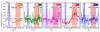 |
Fig. 9 Normalised count rates of He+, C+, N+, O+, and Ne+ plotted as a function of ecliptic longitude for 0.8 <wsw< 1.2 and magnetic configurations φ⊥. Regions in which either the gravitational focusing cone or crescent would produce a significant count rate increase for an interstellar pickup ion are shaded in blue and red, respectively. |
A single PUI does not know whether it originated from the interstellar or inner source, i.e. once injected, its phase-space transport is solely determined by its mass, charge, and position in phase space. This means that, if we measure a single PUI at 1 au, we can only determine theses properties, especially its in situ position in phase space. But we cannot determine where and at what energy it has been injected, because of the unknown history of its phase-space transport prior to its detection. However, if we measure enough particles, a comparison of different PUI species can uncover differences in their phase-space distribution at 1 au that arise from different injection patterns.
There is ample evidence from previous studies that the five ions He+, C+, N+, O+, and Ne+ analysed in this study, actually originate from different sources. He+ and Ne+ probably originate predominantly from interstellar He and Ne, owing to the high FIP of their parent noble gas. Because carbon is believed to be almost fully ionized in the LIC, C+ is generally assumed to receive no contribution from interstellar carbon and is fully attributed to the inner source. The two remaining ions, N+ and O+, are likely to show a mixture of inner and interstellar source. Figure 9 shows the ecliptic longitude distributions of He+, C+, N+, O+, and Ne+ for a relative velocity range of 0.8 <wsw< 1.2 and perpendicular configurations of the local magnetic field vector. Interstellar signatures, like the focusing cone (shaded in blue) and crescent (shaded in red), which are signatures of interstellar species of low and high FIP respectively, are clearly resolved for He+, O+, and Ne+. As mentioned, nitrogen is rather difficult to identify with the mass-per-charge resolution provided by the instrument. This results not only in a poorly resolved torus signature (Fig. 6), but also in a poorly resolved interstellar crescent feature, which should be almost as intense as for O+ bering in mind their similar FIPs. Carbon shows a distribution that is consistent with an isotropic distribution around the Sun without significant count rate increases during periods of the focusing cone or crescent passage of the spacecraft. Thus we can rule out the possibility of a significant amount of interstellar carbon in this wsw range. The recent finding of the interstellar crescent of O+ (Drews et al. 2012) clearly shows a major contribution of interstellar oxygen in the higher wsw range, whereas a comparison of O+ and C+ (Berger et al. 2015) revealed a major contribution to the inner source for the lower wsw range of O+.
Now that we have clarified our expectations for the different origins of He+, C+, N+, O+, and Ne+, we discuss their influence on the observed R(wsw). Interestingly, the similar R(wsw) for He+ and Ne+, shown in Fig. 6, supports our finding in the previous section that resonant wave-particle interaction does not seem to be the main driver for the isotropisation of PUIs. Both ions originate from the interstellar source and, because of their similar FIP, their spatial injection pattern is expected to be similar. Following the argument that Ne+ with a mass-per-charge of 20 amu/e would experience much stronger pitch-angle scattering compared to He+ with mass-per-charge 4 amu/e, the torus feature of Ne+ should be much less pronounced.
Secondly, we compare He+ and C+ since these ions are attributed purely to the interstellar and inner source, respectively. In this context, it is quite surprising that R(wsw) of C+ and He+ look very similar, i.e. the C+ torus signature at wsw ≈ 1.1 has a remarkable resemblance to that from He+ (Fig. 6). Our error estimation, which considers uncertainties resulting from the underlying counting statistics, the ambiguity of the mass-per-charge model, as well as a possible time-of-flight background (Fig. 2), supports our conclusion that the C+signature is, indeed, significant. Nonetheless, the wsw-spectrum of C+ deviates considerably from the wsw-spectrum of the predominantly interstellar He+ and Ne+ pickup ions (Fig. 4) with a much higher relative intensity at low wsws. This confirms that the spatial injection pattern of C+ is quite different from the interstellar source. At wsw< 0.6, on the other hand, He+ and Ne+ seem to be fully isotropic (R(wsw) ≈1), while C+ shows a systematic signature of streaming that is parallel to the ambient solar magnetic field (R(wsw) < 1). As mentioned before, PUI species that are believed to be dominated by an inner-source contribution at wsw< 0.6, i.e. O+ and N+, show the same tendency of R(wsw) at lower wsw.
In summary, our observations of He+ and Ne+ are in agreement with the idea that interstellar PUIs are injected as a torus distribution (R(wsw) > 1), which transforms into a fully isotropic VDF (R(wsw) ≈ 1) at lower wsws, i.e. at longer travel distances owing to an adiabatic cooling of these PUI (Fig. 7). But our observations also indicate that, based on these assumptions, the isotropization happens rapidly after the injection and continues more steadily for travel distances >0.05 au, which cannot be explained by pitch-angle scattering caused by resonant wave-particle interaction. Our C+ observations, on the other hand, are not in agreement with the scenario that has been proposed for interstellar PUIs, i.e. an initial anisotropic VDF that is gradually being isotropized. Instead of a gradual isotropization of the C+ torus signature towards lower wsw, we observe a clear reversal of the anisotropy towards one predominantly streaming that is parallel to the ambient magnetic field. The same behaviour is also observed for O+ and N+, which are both expected to have significant inner-source contributions at wsw< 0.6. Although the detailed nature of the inner source is not sufficiently well understood to make meaningful predictions about the isotropy of these PUIs (Allegrini et al. 2005), our C+ observations of R(wsw) cannot be explained by an initial anisotropy of the distribution that is gradually isotropised by whatever process. An initial anisotropic distribution would either start at R(wsw) < 1 for predominant streaming along the magnetic field or R(wsw) > 1 for torus-like distributions. Any physical process that tends to isotropise the distribution can only push towards R(wsw) = 1, but we observe R(wsw) < 1 at lower wsws and R(wsw) > 1 at higher wsws. Nevertheless, the observed difference in R(wsw) of He+ and C+ at lower wsws is significant and is likely to result from the different injection pattern of both PUI species. The fact that the C+ torus signature is only observed at wsw = 1.1 and looks very similar to the one of He+, tells us that the processes under which a torus distribution is formed or destroyed are the same for C+ and He+ and, in all likelihood, independent of the neutral source population.
Finally we address the significantly higher values of R(wsw) of O+ and N+ in the range 0.8 <wsw< 1.2, i.e. the much stronger torus signature of O+ (and N+) compared to He+, Ne+, and C+. Although we expect O+ (and N+) to behave very similarly, we focus the following discussion on O+ because N+ is, as stated before, poorly resolved. O+ is a mixture of interstellar and inner source PUIs that is likely to be dominated by the interstellar source in the range 0.8 <wsw< 1.2. However, even a contribution of inner source PUIs cannot explain the higher values of R(wsw) = 3 of O+, because He+, Ne+, and C+ all show remarkably similar values of R(wsw) ≈ 2. So not only a difference in the source, but also a systematic trend with mass-per-charge can be ruled out.
One thing that might explain the observations is a difference in the spatial injection pattern of O+ compared to He+, Ne+, and C+. The latter three ions have production rates that peak at r< 1 au. The first two because of their similar high FIP, the last one because all proposed scenarios for the inner source would have a maximum production rate at r< 1 AU. Only for interstellar O+ is the peak production at r> 1 au as is evidenced by the observation of the very noticeable interstellar crescent of O+ (Drews et al. 2015). In the light of the classical assumption of strict adiabatic cooling, Eq. (6), i.e. the observed wsw is sharply connected to the distance the PUI has traversed, R(wsw), would be independent of the spacial injection pattern. This is because PUIs that are observed at a given wsw are believed to have been injected at the same distance to the observer. However, in this study, we have presented evidence that the classical picture for the phase-space evolution of PUIs of resonant wave-particle interaction as the main driver for pitch-angle scatter, combined with adiabatic cooling, is highly oversimplified and cannot explain our observations. If we refrain from the idea of strict adiabatic cooling, the difference in the injection pattern of O+ may produce the observed difference in R(wsw). For He+, Ne+, and C+ we would observe more particles at wsw ≈ 1 that originate closer to the Sun and thus would have had more time to be scattered out of the initial torus distribution. For O+, on the other hand, the situation is closer to the classical assumption, i.e. because of the increasing production rate across 1 au, we see more PUIs that have been generated closer to the spacecraft and thus have had less time to be scattered out of the torus.
6. Conclusions
We have derived wsw-spectra, f(wsw), of He+, C+, N+, O+, and Ne+ using data accumulated over an observation period of six years from the PLASTIC instrument on board STEREO A (Fig. 4). Calculating the ratio of PUI wsw-spectra, R(wsw) = f(wsw)⊥/f(wsw)∥, between two different configurations of the solar magnetic field vector φ⊥ and φ∥ (Fig. 5), allowed us to estimate the anisotropy of the PUI VDF as a function of wsw. Our results show that the anisotropy of the PUI VDF is most distinct at velocities close to the PUI’s injection velocity at wsw ≈ 1. It also seems that the anisotropies at these velocities of He+ (and Ne+) and O+ (and N+) deviate considerably in the sense that a significantly higher fraction of O+ and N+ are still distributed as a torus, compared to He+ and Ne+ (Fig. 6). The same behaviour is also observed for shorter observation periods of one to three months and is therefore unlikely to be connected to specific heliospheric conditions (Fig. 8). Remarkably, we also found a C+ torus at wsw = 1.1, which is statistically significant and not produced by a source of interstellar carbon atoms (Fig. 9). Despite the significantly different production mechanism for inner-source C+, compared to the predominantly interstellar He+, O+, and Ne+ pickup ions, the strong similarity of the C+ torus signature implies that its formation and destruction is tied to the same phase-space transport processes as for He+ and Ne+.
As was already implied in the previous discussion of the C+ torus signature and the scattering mean-free path of O+ and He+, the observed differences (or similarities) in the isotropy of the He+, C+, N+, O+, Ne+ VDF (Fig. 6) cannot be easily explained with an individual view of the PUI phase-space transport. More specifically, following the classic description of the PUI phase space transport via adiabatic deceleration, resonant wave particle interaction and the typical PUI production mechanisms, we were unable to find an individual process or quantity that can explain all our observations, as shown in Fig. 6.
The source population and mechanism for the production of He+, O+, and Ne+, all pickup ions of predominantly interstellar origin, are very similar, while the isotropic part of the O+ VDF differs considerably from that of He+ and Ne+. The same argument applies for C+, which is, in all likelihood, produced by an interaction with the solar wind and nm-sized dust grains (Wimmer-Schweingruber & Bochsler 2003) but nevertheless shows a ratio, R(wsw) that is remarkably similar to those of He+ and Ne+ (Fig. 6). As a consequence, it is unlikely that the source population or production mechanism of these ions significantly impact the isotropization of the PUI VDF. Another controlling factor for the isotropization of the PUI VDF might be the mass per charge of the respective ion, i.e. the resonance frequency which determines the available power for the resonant wave-particle interaction. If resonant wave-particle interactions really were the pivotal process for the isotropization of the PUI VDF, there should be a significant decrease in the anisotropy of the PUI VDF with increasing PUI mass per charge (He→C→N→O→Ne). However, our observations show an increased VDF anisotropy for O+ (and N+), while the level of anisotropy for all other ions is roughly the same. In this context, it is also highly unlikely that resonant wave-particle interaction is the sole controlling factor for the isotropization of the PUI VDF. Finally, the FIP, which determines the in situ production of these ions by solar UV radiation, might play a role in the formation of the initial torus-distributed pickup ion VDF. But again, with He and Ne being low FIP ions, and C, N, and O being high FIP ions, no evident correlation between an atom’s FIP and the anisotropy of the respective PUI species was observed.
In summary, it is unlikely that our observations shown in Fig. 6 can be explained with a classic description of the PUI phase-transport process via adiabatic deceleration, specifically that the injection location is tied to the observed pickup ion wsw, resonant wave-particle interaction and the PUI’s source population. There is, however, one controlling parameter that is capable of explaining the observed VDF anisotropy presented in Fig. 6, which is tied to an ion’s FIP and its production mechanism. Because of their low FIP, He+ and Ne+ have a maximum production rate at r< 1 au. While C+ also has a maximum production well inside 1 au owing to its production scenario that requires a sufficient interaction of solar wind ions with nm-sized dust particles (Taut et al. 2015). In contrast, because of the higher FIP, N+ and O+ have a maximum production rate that lies well beyond 1 au, which in turn means that their production rate increases from the Sun to an observer at 1 au. In other words, observations of He+, C+, and Ne+ predominantly stem from pickup ions being produced closer to the Sun than N+ and O+, which are primarily produced closer to the observer. In the context of an adiabatic deceleration mechanism (Eq. (6)) acting on the PUI VDF, the injection profile of a PUI seems rather unimportant, i.e. a PUI observed at its injection velocity (0.9 <wsw< 1.1) is always produced close to the observer, and mainly determines the shape of the PUI VDF. If, however, the correlation between the PUI injection location and the observed PUI wsw is not as close as expected from an idealised adiabatic deceleration (Eq. (6)), it is evident that the injection profile might play a much more important role for the state of anisotropy of the PUI VDF. Pickup ions that are produced predominantly close to the Sun (He+, C+, Ne+) have undergone more pitch-angle-scattering processes than PUIs produced closer to the observer (N+ and O+), but do not necessarily have systematically smaller velocities wsw as a result of an adiabatic deceleration.
On a final note, we also emphasise that the mathematical formalism of either adiabatic or magnetic cooling mechanisms cannot easily be applied to a PUI population that is highly anisotropic (Fahr 2007). Initial anisotropies of the PUI VDF in the form of a torus mean that the guiding centre velocity of this type of PUI population that is injected at non-perpendicular magnetic field configuration is slower than vsw (see Fig. 10 and Drews et al. 2015). In other words, a torus-distributed PUI VDF will lead to drifts relative to the solar wind plasma parcel in which the PUIs were produced and will therefore lead to highly complex and dynamic interactions with the ambient and generally time-dependent solar wind plasma. Because the observed anisotropies of He+ and O+ (Fig. 6) are not fully consistent with the idea of a resonant interaction with the fluctuating solar magnetic field, it is likely that drifts of the torus’ guiding centre velocities, with respect to vsw, are also important for the isotropization of the PUI VDF. In this context, it is also questionable whether a simplified approximation of the PUI phase-space transport (see Fig. 7) via an adiabatic or magnetic deceleration mechanism and a single parameter for the PUI pitch-angle scattering behaviour is really sufficient to describe the physics of the PUI transport.
Admittedly, we do not provide or elaborate on an alternative for the description of the PUI phase-space transport. It is far beyond the scope of one individual study, and the mathematical treatment would have to allow highly anisotropic VDFs, such as a torus distribution. It is therefore very possible that numerical simulations that treat ensembles of particles will ultimately provide the most accurate description of the PUI transport. We have, however, provided observational evidence that an idealized description of the PUI transport via adiabatic deceleration, a mechanism that was originally introduced to describe the phase-space transport of cosmic rays (Parker 1965), might not be sufficient to describe the transport of PUIs.
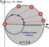 |
Fig. 10 Velocity space diagram of He+ torus distributions (red) at different configurations of the solar magnetic field. Corresponding guiding centre velocities of the respective distributions are shown as blue circles. The solar wind speed is shown as a green circle. Evidently, the torus’ guiding centre velocity equals the solar wind speed only for magnetic configurations where φB = ± 90° (see also Fig. 5). |
Acknowledgments
We would like to thank the PLASTIC and IMPACT teams for providing the necessary data for this work (Galvin et al. 2008 and Acuña et al. 2008). Part of this work was supported by the German Deutsche Forschungsgemeinschaft, DFG (project number: Wi2139/7-1).
References
- Acuña, M. H., Curtis, D., Scheifele, J. L., et al. 2008, 136, 203 [Google Scholar]
- Allegrini, F., Schwadron, N. A., McComas, D. J., Gloeckler, G., & Geiss, J. 2005, J. Geophys. (Space Phys.), 110, 5105 [NASA ADS] [CrossRef] [Google Scholar]
- Berger, L., Wimmer-Schweingruber, R. F., & Gloeckler, G. 2011, Phys. Rev. Lett., 106, 151103 [NASA ADS] [CrossRef] [Google Scholar]
- Berger, L., Drews, C., Taut, A., & Wimmer-Schweingruber, R. F. 2013, AIP Conf. Ser., 1539, 386 [NASA ADS] [CrossRef] [Google Scholar]
- Berger, L., Drews, C., Taut, A., & Wimmer-Schweingruber, R. F. 2015, A&A, 576, A54 [NASA ADS] [CrossRef] [EDP Sciences] [Google Scholar]
- Bruno, R., & Carbone, V., 2013, Liv. Rev. Sol. Phys., 10, 2 [Google Scholar]
- Cannon, B. E., Smith, C. W., Isenberg, P. A., et al. 2014, ApJ, 784, 150 [NASA ADS] [CrossRef] [Google Scholar]
- Chalov, S. V. 2014, MNRAS, 443, L25 [NASA ADS] [CrossRef] [Google Scholar]
- Chalov, S. V., & Fahr, H. J. 1996, Sol. Phys., 168, 389 [NASA ADS] [CrossRef] [Google Scholar]
- Chalov, S. V., & Fahr, H. J. 1998, A&A, 335, 746 [NASA ADS] [Google Scholar]
- Chalov, S. V., & Fahr, H. J. 1999, Sol. Phys., 187, 123 [NASA ADS] [CrossRef] [Google Scholar]
- Chen, J. H., Möbius, E., Gloeckler, G., et al. 2013, J. Geophys. Res., 118, 3946 [NASA ADS] [CrossRef] [Google Scholar]
- Cummings, A. C., Stone, E. C., & Steenberg, C. D. 2002, ApJ, 578, 194 [NASA ADS] [CrossRef] [Google Scholar]
- Drews, C., Berger, L., Wimmer-Schweingruber, R. F., et al. 2010, J. Geophys. Res., 115, 10108 [CrossRef] [Google Scholar]
- Drews, C., Berger, L., Wimmer-Schweingruber, R. F., et al. 2012, J. Geophys. Res., 117, 9106 [Google Scholar]
- Drews, C., Berger, L., Wimmer-Schweingruber, R. F., & Galvin, A. B. 2013, Geophys. Res. Lett., 40, 1468 [NASA ADS] [CrossRef] [Google Scholar]
- Drews, C., Berger, L., Taut, A., Peleikis, T., & Wimmer-Schweingruber, R. F. 2015, A&A, 575, A97 [NASA ADS] [CrossRef] [EDP Sciences] [Google Scholar]
- Fahr, H. J. 2007, Ann. Geophys., 25, 2649 [NASA ADS] [CrossRef] [Google Scholar]
- Fahr, H. J., & Fichtner, H. 2011, A&A, 533, A92 [NASA ADS] [CrossRef] [EDP Sciences] [Google Scholar]
- Fisk, L. A., & Gloeckler, G. 2012, Space Sci. Rev., 173, 433 [NASA ADS] [CrossRef] [Google Scholar]
- Fisk, L. A., Schwadron, N. A., & Gloeckler, G. 1997, Geophys. Res. Lett., 24, 93 [Google Scholar]
- Galvin, A. B., Kistler, L. M., & Popecki, M. A. 2008, Space Sci. Rev., 136, 437 [NASA ADS] [CrossRef] [Google Scholar]
- Geiss, J., Gloeckler, G., Fisk, L. A., & von Steiger, R. 1995, J. Geophys. Res., 100, 23373 [NASA ADS] [CrossRef] [Google Scholar]
- Gloeckler, G., & Geiss, J., 2001, Space Sci. Rev., 97, 169 [NASA ADS] [CrossRef] [Google Scholar]
- Gloeckler, G., Schwadron, N. A., Fisk, L. A., & Geiss, J. 1995, Geophys. Res. Lett., 22, 2665 [NASA ADS] [CrossRef] [Google Scholar]
- Gloeckler, G., Fisk, L. A., Geiss, J., Schwadron, N. A., & Zurbuchen, T. H. 2000, J. Geophys. Res., 105, 7459 [NASA ADS] [CrossRef] [Google Scholar]
- Hilchenbach, M., Hovestadt, D., Klecker, B., & Moebius, E. 1992, in Solar Wind Seven Colloquium, 349 [Google Scholar]
- Hovestadt, D., Hilchenbach, M., Bürgi, A., et al. 1995, Sol. Phys., 162, 441 [NASA ADS] [CrossRef] [Google Scholar]
- Isenberg, P. A. 1987, J. Geophys. Res., 92, 1067 [NASA ADS] [CrossRef] [Google Scholar]
- Isenberg, P. A. 1997, J. Geophys. Res., 102, 4719 [NASA ADS] [CrossRef] [Google Scholar]
- Kallenbach, R., Geiss, J., Gloeckler, G., & von Steiger, R. 2000, Ap&SS, 274, 97 [NASA ADS] [CrossRef] [Google Scholar]
- Mann, I., & Czechowski, A. 2005, ApJ, 621, L73 [NASA ADS] [CrossRef] [Google Scholar]
- Mann, I., Meyer-Vernet, N., & Czechowski, A. 2013, Phys. Rep., 536, 1 [Google Scholar]
- Marsch, E., Rosenbauer, H., Schwenn, R., Muehlhaeuser, K.-H., & Denskat, K. U. 1981, J. Geophys. Res., 86, 9199 [NASA ADS] [CrossRef] [Google Scholar]
- Moebius, E., Hovestadt, D., Klecker, B., Scholer, M., & Gloeckler, G. 1985, Nature, 318, 426 [NASA ADS] [CrossRef] [Google Scholar]
- Moebius, E., Klecker, B., Hovestadt, D., & Scholer, M. 1988, Ap&SS, 144, 487 [NASA ADS] [Google Scholar]
- Moebius, E., Rucinski, D., Hovestadt, D., & Klecker, B. 1995, A&A, 304, 505 [NASA ADS] [Google Scholar]
- Möbius, E., Rucinski, D., Lee, M. A., & Isenberg, P. A. 1998, J. Geophys. Res., 103, 257 [NASA ADS] [CrossRef] [Google Scholar]
- Möbius, E., Bzowski, M., Chalov, S., et al. 2004, A&A, 426, 897 [NASA ADS] [CrossRef] [EDP Sciences] [Google Scholar]
- Oka, M., Terasawa, T., Noda, H., Saito, Y., & Mukai, T. 2002, Geophys. Res. Lett., 29, 1612 [NASA ADS] [CrossRef] [Google Scholar]
- Parker, E. N. 1965, Planet. Space Sci., 13, 9 [Google Scholar]
- Rucinski, D., & Fahr, H. J. 1989, A&A, 224, 290 [NASA ADS] [Google Scholar]
- Rucinski, D., Bzowski, M., & Fahr, H. J. 2003, Ann. Geophys., 21, 1315 [Google Scholar]
- Saul, L., Möbius, E., Isenberg, P., & Bochsler, P. 2007, ApJ, 655, 672 [NASA ADS] [CrossRef] [Google Scholar]
- Saul, L., Wurz, P., & Kallenbach, R. 2009, ApJ, 703, 325 [NASA ADS] [CrossRef] [Google Scholar]
- Schippers, P., Meyer-Vernet, N., Lecacheux, A., et al. 2015, ApJ, 806, 77 [NASA ADS] [CrossRef] [Google Scholar]
- Schwadron, N. A., Geiss, J., Fisk, L. A., et al. 2000, J. Geophys. Res., 105, 7465 [NASA ADS] [CrossRef] [Google Scholar]
- Semar, C. L. 1970, J. Geophys. Res., 75, 6892 [NASA ADS] [CrossRef] [Google Scholar]
- Schwadron, N. A. 1998, J. Geophys. Res., 103, 20643 [NASA ADS] [CrossRef] [Google Scholar]
- Taut, A., Berger, L., Drews, C., & Wimmer-Schweingruber, R. F. 2015, A&A, 576, A55 [NASA ADS] [CrossRef] [EDP Sciences] [Google Scholar]
- Vasyliunas, V. M., & Siscoe, G. L. 1976, J. Geophys. Res., 81, 1247 [NASA ADS] [CrossRef] [Google Scholar]
- Wenzel, K.-P., Sanderson, T. R., Richardson, I. G., et al. 1986, Geophys. Res. Lett., 13, 861 [NASA ADS] [CrossRef] [Google Scholar]
- Wimmer-Schweingruber, R. F., & Bochsler, P. 2003, Geophys. Res. Lett., 30, 1077 [NASA ADS] [CrossRef] [Google Scholar]
All Tables
Parameters of the mass-per-charge model, I(m/q), for the individual heavy pickup ion species
Definition of the magnetic configurations φ⊥ and φ∥ in which PLASTIC can and cannot observe the pickup ion torus distribution respectively.
Mean travel distance, Λ, after which 80% of He+ and O+ pickup ions are distributed isotropically in velocity space for three different cooling indices, γ.
All Figures
|
Fig. 1 Velocity space diagrams of a pickup ion torus distribution as a (vx,vy)-projection (top left panel) and in the vz = 0 km s-1 plane (top right) are shown for a magnetic configuration in which B is almost perpendicular. Here, vx, vy, and vz are the three vector components of vion, whereas vx is the velocity parallel to vsw. The bottom two panels show the torus distribution under the influence of pitch-angle scattering (right) and adiabatic cooling (left). To illustrate the torus character of the distribution, the (vx,vy)-plane is slightly tilted in this diagram. |
| In the text | |
|
Fig. 2 Mass-per-charge spectrum of heavy pickup ions (Δm/q = 0.4 amu/e) observed by PLASTIC on board STEREO A. The data was accumulated for a period of 2400 days, beginning in March 2007, and C+ velocities of wsw,C+> 0.2 (open circles). A mass-per-charge model (dashed black line) was fitted to the data to obtain the absolute abundances of C+, N+, O+, Fe3+, Ne+, Mg+, and Fe2+ in terms of instrumental count rates. An exponential model was included to estimate and incorporate the influence of instrumental background to the mass-per-charge spectrum between 10 <m/q< 35 amu/e. |
| In the text | |
|
Fig. 3 Mass-per-charge spectra of heavy pickup ions obtained by PLASTIC on STEREO A for three different time periods in which either O+, C+, or Ne+ show a significantly increased abundance compared to other heavy pickup ions (panels from left to right respectively). These periods were used to obtain the necessary parameters for the mass-per-charge model (Eq. (2)) that is used to obtain the heavy pickup ion wsw-spectra. |
| In the text | |
|
Fig. 4 Pickup ion velocity spectra, f(w), of He+, C+, O+, and Ne+ as a function of wsw = | vion−vsw | /vsw. Due to systematic and statistical uncertainties of the underlying mass-per-charge model, a reliable prediction for the velocity spectra of Fe3+, Mg+, and Fe2+ (and partially N+) is hardly possible. The spectra were corrected for the orbital velocity of the spacecraft and instrumental phase space coverage, but no instrumental response function to correct for the varying detection efficiency was applied (see text for details). |
| In the text | |
|
Fig. 5 Illustration of the two different magnetic configurations (inner circle) and corresponding pickup ion torus configuration (outer circle) used throughout this work. For the configuration φ⊥, i.e. the magnetic field vector B points in the direction of the orange shaded area within the inner circle, the pickup ion torus is located in a region of velocity space where it can be detected by the instrument (outer orange shaded ring). For the configuration φ∥, the torus lies exclusively outside the instrument’s aperture and cannot be detected (outer violet shaded ring). The torus distribution, shown in this diagram (red line), corresponds to the magnetic field vector drawn in red. |
| In the text | |
|
Fig. 6 The ratio, R(wsw) (Eq. (5)), of the pickup ion flux as a function of wsw between magnetic configurations φ⊥ and φ∥ for He+, C+, N+, O+, and Ne+ (panels from left to right). The data was collected between March 2007 and December 2013 during periods in which the solar wind velocity was below 450 km s-1. As illustrated in Fig. 5, the magnetic configurations φ⊥ and φ∥ correspond to configurations in which the pickup ion torus lies inside and outside the instrument’s aperture respectively. The ratio f(w)⊥/f(w)∥ is therefore an indicator of the relative flux increase induced by the pickup ion torus distribution or, in more general terms, an indicator for the anisotropy of the pickup ion VDF. |
| In the text | |
|
Fig. 7 The fraction of isotropically distributed pickup ions as a function of their travel distance from their production location up to 1 AU. The travel distance was calculated based on the assumption of an ideal adiabatic expansion with a cooling index of 3/2. Circular and square markers respectively denote whether the anisotropy is produced by pickup ions that stream in predominately perpendicular way or parallel to the local magnetic field. |
| In the text | |
|
Fig. 8 The fraction of isotropically distributed He+ (yellow) and O+ (red) pickup ions at r0 as a function of time (He: Δt = 30 d, O: Δt = 100 d). The solid and dashed lines denote the average and standard deviation of ψ(r0), respectively. |
| In the text | |
|
Fig. 9 Normalised count rates of He+, C+, N+, O+, and Ne+ plotted as a function of ecliptic longitude for 0.8 <wsw< 1.2 and magnetic configurations φ⊥. Regions in which either the gravitational focusing cone or crescent would produce a significant count rate increase for an interstellar pickup ion are shaded in blue and red, respectively. |
| In the text | |
|
Fig. 10 Velocity space diagram of He+ torus distributions (red) at different configurations of the solar magnetic field. Corresponding guiding centre velocities of the respective distributions are shown as blue circles. The solar wind speed is shown as a green circle. Evidently, the torus’ guiding centre velocity equals the solar wind speed only for magnetic configurations where φB = ± 90° (see also Fig. 5). |
| In the text | |
Current usage metrics show cumulative count of Article Views (full-text article views including HTML views, PDF and ePub downloads, according to the available data) and Abstracts Views on Vision4Press platform.
Data correspond to usage on the plateform after 2015. The current usage metrics is available 48-96 hours after online publication and is updated daily on week days.
Initial download of the metrics may take a while.