| Issue |
A&A
Volume 696, April 2025
|
|
|---|---|---|
| Article Number | A107 | |
| Number of page(s) | 25 | |
| Section | Numerical methods and codes | |
| DOI | https://doi.org/10.1051/0004-6361/202453404 | |
| Published online | 09 April 2025 | |
Dust and gas modeling in radiative transfer simulations of disc-dominated galaxies with RADMC-3D
1
Département d’Astronomie, Université de Genève, Chemin Pegasi 51,
1290
Versoix, Switzerland
2
Department of Astrophysics, University of Zurich,
Winterthurerstrasse 190,
8057
Zürich, Switzerland
★ Corresponding author; This email address is being protected from spambots. You need JavaScript enabled to view it.
Received:
11
December
2024
Accepted:
18
February
2025
Abstract
Context. Bridging theory and observations is a key task in modern astrophysics, aimed at improving our understanding of the formation and evolution of galaxies. With the advent of state-of-the-art observational facilities, the accurate modeling of galaxy observables via radiative transfer simulations coupled to hydrodynamic simulations of galaxy formation must be performed.
Aims. We present a novel pipeline, dubbed RTGen, based on the Monte Carlo radiative transfer code RADMC-3D. We explore the impact of the physical assumptions and modeling of dust and gas phases on the resulting galaxy observables. In particular, we thoroughly addressed the impact of the dust abundance, composition, and grain size. We also implemented approximate models for the atomic-to-molecular transition and studied the resulting emission from molecular gas.
Methods. We applied a Monte Carlo radiative transfer a posteriori to determine the dust temperature in six different hydrodynamic simulations of isolated galaxies. Afterwards, we applied ray tracing to compute the spectral energy distribution (SED), as well as to derive the continuum images and spectral line profiles.
Results. We find that our pipeline is able to predict accurate SEDs for the studied galaxies, along with the continuum and CO luminosity images. These results are in good qualitative agreement with literature results from both observations and theoretical studies. In particular, we find the dust modeling to have an important impact on the convergence of the resulting predicted galaxy observables and that an adequate modeling of dust grain composition and size is required.
Conclusions. We conclude that our novel framework is ready to perform high-accuracy studies of the observables of the interstellar medium (ISM), reaching a convergence of a few tens of percent under the studied baseline configuration. This will enable robust studies of galaxy formation and, in particular, the nature of massive clumps in high-redshift galaxies thanks to the generation of reliable and accurate mock images mimicking observations from state-of-the-art facilities, such as JWST and ALMA.
Key words: methods: numerical / galaxies: evolution / galaxies: formation / galaxies: ISM
© The Authors 2025
 Open Access article, published by EDP Sciences, under the terms of the Creative Commons Attribution License (https://creativecommons.org/licenses/by/4.0), which permits unrestricted use, distribution, and reproduction in any medium, provided the original work is properly cited.
This article is published in open access under the Subscribe to Open model. This email address is being protected from spambots. You need JavaScript enabled to view it. to support open access publication.
1 Introduction
The advent of modern astronomical ground-based and space telescopes probing a large portion of the electromagnetic spectrum has triggered an unprecedented recent advancement in the understanding of the processes shaping galaxy formation and evolution. In particular, the James Webb Space Telescope (JWST; Gardner et al. 2006) and the Atacama Large Millime- ter/submillimeter Array (e.g., Wootten & Thompson 2009), as well as optical telescopes such as the Very Large Telescope (VLT1), the twin Keck2 telescopes, and the Subaru telescope3 have delivered unprecedented high-resolution photometric and spectroscopic observations up to high redshifts, with the highest redshift galaxy that has been spectroscopically confirmed to date found at ɀ ~ 14.32 (Robertson et al. 2024).
Nonetheless, developing a solid theoretical understanding of the empirical measurements is not a trivial task due to the high degree of complexity and nonlinearity of the physical processes involved. In this sense, numerical simulations represent the ideal tool for investigating galaxy formation and evolution from a theoretical perspective. Over recent decades, a huge effort has been undertaken to refine hydrodynamic simulations and enable them to reproduce the observed properties with great accuracy (see, e.g., Vogelsberger et al. 2020; Crain & van de Voort 2023, for detailed reviews). Despite the general success in this field, simulations have to cope with the complex problem of dealing with a wide range of different scales and a huge dynamical range. In fact, achieving both high resolution and large volume is computationally prohibitive even for modern world-class supercomputing facilities. In particular, the resolution is typically not large enough to simulate all the involved physical processes down to parsec scales. As such, a vast range of physical phenomena are modeled in a subgrid fashion, by adopting prescriptions that strive to mimic the effect of such processes, despite the lack of an adequate resolution to properly resolve them.
In this context, properly simulating the phenomena involving the interaction between radiation and matter and the transport of energy and momentum happening thereof would imply solving the equations of radiative transfer at all the steps of the simulations, which would make the computation even more costly. In fact, while there are some cases where the radiative transfer is solved on-the-fly in hydrodynamic simulations (e.g., Gnedin & Abel 2001; Gnedin et al. 2009; Gnedin & Kravtsov 2010; Lupi et al. 2018; Rosdahl et al. 2018; Kannan et al. 2022) in the vast majority of the cases, the computation is performed a posteriori. In particular, a posteriori radiative transfer simulations are based on the assumption that radiation propagates at much faster speed than that inferred from typical dynamical time scales involved in the motion of matter; hence, we can simulate the radiative transfer following the propagation of photons at frozen time, neglecting the potential micro-motion of matter meanwhile. In this sense, a number of radiative transfer codes have been presented in the literature, achieving great accuracy and becoming a standard in the generation of mock images and spectra to perform galaxy formation and evolution studies, such as TRAPHIC (Pawlik & Schaye 2008), RADMC-3D (Dullemond et al. 2012), DESPOTIC (Krumholz 2014), SKIRT (Camps & Baes 2015; Baes & Camps 2015; Camps & Baes 2020), CLOUDY (Ferland et al. 1998, 2017), ART2 (Li et al. 2020), and Powderday (Narayanan et al. 2021), amongst others.
In this paper, we present a novel pipeline (dubbed RTGen) to perform end-to-end a posteriori radiative transfer of galaxy simulations, including both dust continuum and spectral line transfer computations. In particular, we rely on the RADMC-3D code (Dullemond et al. 2012), a highly-flexible software performing Monte Carlo simulations to determine the dust temperature and ray-tracing photons by solving the radiative transfer equation afterwards. In particular, we first show how to obtain continuum images at arbitrary wavelengths as well as the full spectral energy distribution (SED). Afterwards, we present our modeling of the atomic-to-molecular transition to split the atomic and molecular phases of the gas. Eventually, we combine the previous techniques to predict images of CO fine-structure transitions. To address the variations between different simulations and investigated models, we compare both the predicted SEDs and images, as well as the distribution results for different quantities when relevant.
The paper is organized as follows. Section 2 presents the suite of simulations used as simulated sample in this work. Section 3 summarizes the modeling of the various physical components that we carry out. Section 4 presents the analysis of the main results and Sect. 5 discusses the time evolution of the predicted observables. We present our conclusions in Sect. 6.
2 Hydrodynamic simulations of isolated galaxies
In this section, we briefly summarize the simulations adopted throughout this work. We refer to Tamburello et al. (2015) for a detailed description of the setup and the general results.
The suite of simulations presented in Tamburello et al. (2015) comprises 28 simulations spanning 11 different models of galaxy structural parameters. The simulations were run using GASOLINE2 (Wadsley et al. 2017), a more recent version of the original N-body + smoothed particle hydrodynamics (SPH) code GASOLINE (Wadsley et al. 2004). GASOLINE2 adopts a binary tree structure to compute pair-wise gravitational interactions and smooths the gravitational force using a spline kernel function. The equations of hydrodynamics are solved relying on the SPH Lagrangian formulation and include radiative and Compton cooling, as well as subgrid models for star formation, supernova feedback, and metal enrichment from the explosion of supernovae and stellar winds. Radiative cooling is implemented for a mixture of hydrogen, helium, and metals, where collisional ionization equilibrium (CIE) is assumed for the latter (but not for hydrogen and helium) and modeled according to the tabulated data from Shen et al. (2010, 2013), who assumed CIE using the CLOUDY code (Ferland et al. 1998) and set a cooling temperature floor Tmin = 10 K. In the feedback model adopted for this suite of simulations, known as the “blastwave model” (Stinson et al. 2006), cooling is switched off inside the radius of the blastwave produced by the explosion of supernovae type II for a time interval ∆t ~ 10–30 Myr, but it is not disabled in supernovae type I explosions.
Star formation is triggered in gas particles which (i) have density ρ > 10mH cm−3, where mH is the hydrogen mass; (ii) have temperature T < 3 × 10⁴ K; and (iii) are part of converging flow. The star formation rate (SFR) in star-forming particles is assigned according to a Schmidt law and newly formed stars are sampled from a Kroupa (2001) initial mass function (IMF).
Such subgrid prescriptions for star formation and feedback were proven to be capable of reproducing the properties of galaxies across a large dynamical range and a variety of morphological types. As stressed in Tamburello et al. (2015), this indicates that the adopted models (while being purely phenomenological) encapsulate the salient features of the energetics of the processes shaping galaxy formation and, hence, they directly impact the stability of forming discs. This aspect is crucial to reliably study the processes responsible for the formation and phenomenology of giant clumps (massive star-forming regions) as done in Tamburello et al. (2015), 2017) and will be done in a companion paper.
The initial conditions of the simulations were set up as in Mayer et al. (2001, 2002) following the original method by Hernquist (1993). In particular, the models were made up of a dark matter halo following the radial density profile from Navarro et al. (1997); NFW and embedding a disc with both stellar and gas components, exploring a range of structural parameters. While these simulations consist of high-resolution, non-cosmological simulations of isolated galaxies, the initial conditions were set up in such a way to mimic the features of cosmological simulations. In particular, Tamburello et al. (2015) chose a sample of 12 massive isolated galaxies at 3.8 < ɀ < 5.2 from the ARGO simulation (Feldmann & Mayer 2015; Fiacconi et al. 2015) in an epoch when they are still in the outskirts of the main host and not experiencing mergers.
All simulations were run adiabatically for ∆t = 1 Gyr to allow the galaxies to relax and achieve stability. After the relaxation phase, all discs were stable, with the Toomre (1964) parameter of Q > 1 in all the simulations and all over the simulated volume. Afterwards, the simulations were run for ∆t = 2 Gyr more, switching on radiative cooling and other subgrid physics models (see details below). As stated by Tamburello et al. (2015), assuming that galaxies are initialized at ɀ ~ 3, after the relaxation phase, they should represent discs at ɀ ~ 2.
The 11 different models studied here are summarized in Table 1 of Tamburello et al. (2015). In particular, they consist of adopting different sets of values of the following parameters:
velocity at the virial radius of the halo Vvir: set to be in the range 100 < Vvir < 180 km s−1, to match the asymptotic velocity of the most massive galaxies in ARGO (Fiacconi et al. 2015);
NFW halo concentration c: set to be in the range 6 < c < 15 (e.g., Bullock et al. 2001; Ludlow et al. 2014), with c = 6 constituting the most representative case for the studied galaxies;
gas fraction of ƒgas = Mgas/(Mgas + Mstar): set to either ƒgas = 0.3 – an intermediate value in the selected ARGO galaxies (Fiacconi et al. 2015) – or fgas = 0.5, as favoured by observations of galaxies at cosmic noon (e.g., Dessauges-Zavadsky et al. 2015; Tacconi et al. 2020);
inclusion of feedback (FB);
inclusion of metal cooling (MC);
inclusion of metal thermal diffusion (MTD);
adoption of the Geometric Density SPH (GDSPH);
number of particles;
softening length ϵ: set to either ϵ = 50 pc or ϵ = 100 pc.
Out of the 28 simulations, 22 were run at low resolution, using np,dm = 1.2 × 10⁶ dark matter particles, np,gas = 105 gas particles, and np,s = 105 star particles, while the remaining 6 simulations were run at a higher resolution, employing np,dm = 2 × 10⁶ and np,gas = np,s = 106.
In this work, we consider six simulations, with different values for Vvir, c, fgas , cooling, number of particles, and ϵ. However, all the considered runs include feedback and none of them feature MTD nor GDSPH. In particular, the features of the chosen simulations are summarized in Table 1, a simplified version of Table 2 of Tamburello et al. (2015) restricted to just the simulations used herein.
Figures 1 and 2 show the gas mass and stellar mass surface density maps of the studied simulations, respectively, viewed face-on, after ∆t = 0.2 Gyr from the end of the relaxation phase. As can easily be noticed, the discs display different morphologies and clumpiness properties, depending on the physics models and the structural parameters adopted in each simulation. In particular, runs 13, 16, and 23 feature a smooth regular disc, whereas runs 25, 26, and 27 display the presence of clumps, as a result of the higher gas fraction used in the simulation, which favours fragmentation (Tamburello et al. 2015).
Summary of the parameters adopted in the simulations used in this work.
3 Radiative transfer with RADMC-3D
RADMC-3D4 (Dullemond et al. 2012) is a software package designed to perform radiative transfer simulations in astrophysical problems defined on an Eulerian grid of arbitrary geometry. The code first performs a Monte Carlo run to determine the dust temperature, and subsequently ray-traces the photons of specified wavelength along the line of sight. In particular, both continuum and atomic and molecular spectral line radiative transfer are implemented in RADMC-3D. We review the basic working principles underlying RADMC-3D, including a detailed description of Monte Carlo radiative transfer, in Appendix A. We refer to Steinacker et al. (2013); Noebauer & Sim (2019) for a more complete review of Monte Carlo radiative transfer techniques.
Importantly, RADMC-3D does not include any built-in model for the physical system to be simulated. Hence, the practitioner should supply to the code all the inputs of the computation to be performed, specifically related to the (more details on this given later in this paper):
gas mass density;
stellar mass density or the position of single stars, depending on the complexity of the problem and the number of total stars, as well as the effective temperature and radius of the stars;
dust mass density.
In particular, as discussed in more detail in Sect. 3.5, the input fields must be supplied in a grid format. This implies that a suitable interpolation of particles onto a mesh must be performed in the case of SPH simulations.
For these reasons, an additional amount of work is required on the side of the user. However, this reflects into a great flexibility, as the user is not bound to any predefined model and is thus able to vastly explore the associated parameter space. In this paper (the first of a series), we focus on the study of the different assumptions and modeling of the resulting observable features of galaxies. In particular, we performed a variety of experiments changing the underlying physical assumptions and quantifying the differences by computing the SED, as well as images of the continuum at fixed wavelengths and of selected spectral lines. In the following, we present the modeling of the different physical components of the interstellar medium (ISM), needed as inputs to RADMC-3D.
3.1 Dust modeling
Modeling the dust in a numerical simulation is a non-trivial task, which involves tracking the detailed evolution of the formation, growth, and destruction of dust grains (see, e.g., Aoyama et al. 2017; Davé et al. 2019; Esmerian & Gnedin 2022; Dubois et al. 2024, and references therein).
In the simulations we use in this work, there is no on-the- fly dust modeling; hence, we need to model it a posteriori. In what follows, we present our modeling of the dust and discuss the different implemented models and options. While this certainly offers an additional degree of freedom (and, hence, a source of potential uncertainty), we show here that it is very instructive to study a few representative cases to understand how sensitive the predicted observables from radiative transfer simulations are to the underlying model for the dust. In particular, we present the relevant models for the dust abundance, composition, and grain size. We stress that henceforth our framework does not include polycyclic aromatic hydrocarbon emission from stochastically heated small dust grains (see, e.g., Camps & Baes 2015).
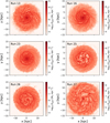 |
Fig. 1 Gas mass surface density maps, viewed face-on, for the six different runs analyzed in this paper, after ∆t = 0.2 Gyr from the end of the relaxation phase. The run each projection refers to is reported inside the corresponding panel. |
3.1.1 Dust abundance
As anticipated, the dust abundance (i.e., the number of grains and their mass) in a given spatial region of the simulation is the result of a complex balance between dust grain formation, growth, and destruction. Here, since these processes are not modeled inside our simulations, we made use of literature results and performed our modeling a posteriori. In particular, we relied on the results by Li et al. (2019), who found the relation between the dust-to-gas ratio (DGR) and the metallicity (Z) from the SIMBA simulation to be just weakly dependent on redshift from ɀ = 0 to ɀ = 6; this is also in reasonable agreement with observations (e.g., Rémy-Ruyer et al. 2014; Zanella et al. 2018; De Vis et al. 2019; Péroux & Howk 2020; Popping & Péroux 2022; Valentino et al. 2024, and references therein). In particular, we adopted the following scaling relation (Li et al. 2019):
 (1)
(1)
with a scatter of σDGR ~ 0.31 dex. While this relation was originally fitted by relating the mean global DGR and metallicity for a large and diverse sample of galaxies, we assume here that it holds cell by cell in a spatially resolved fashion. This approach allows us to capture at least the dependence of the DGR on the gas metallicity. It has been shown that the DGR strongly varies as a function of gas properties beyond metallicity, such as the density and temperature (see, e.g., Dubois et al. 2024). However, in our simulations, the cold phase of the ISM is not resolved; therefore, it is not meaningful to incorporate these dependencies in our model. In this way, we first predicted a DGR value for each cell given the metallicity therein and, subsequently, added a random component to mimic the scatter, randomly sampled from a log-normal distribution with σ = σDGR. Assuming the validity of such a scaling relation at the cell level allows the model to have an additional degree of freedom, with respect to assuming a fixed DGR throughout the galaxy. We also recall here that these tests are performed mostly as proofs of concept, but that the flexibility of our framework would (in principle) allow us to arbitrarily vary the assumed model and explore different scenarios. We restrict our study here to the two cases mentioned above. We also notice that the adoption of MTD in the simulations may have a significant impact on the spatial distribution of the metal- licity and could consequently affect the cell-wise value of the DGR. We leave a more thorough investigation of these aspects related to the modeling of the DGR for future publications.
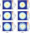 |
Fig. 2 Stellar mass surface density maps, viewed face-on, for the six different runs analyzed in this paper, after ∆t = 0.2 Gyr from the end of the relaxation phase. The run each projection refers to is reported inside the corresponding panel. |
3.1.2 Dust composition
The interstellar dust is formed from elements expelled by stars undergoing the asymptotic giant branch (AGB) phase (e.g., Marigo 2001; Ferrarotti & Gail 2006; Schneider et al. 2014; Goldman et al. 2022; Dell’Agli et al. 2023) and from supernovae explosions (e.g., Todini & Ferrara 2001; Nozawa et al. 2007, 2011; Sarangi & Cherchneff 2015; Gall & Hjorth 2018). The two main constituents of the interstellar dust are silicate and carbonaceous grains (oxygen-rich and carbon-rich, respectively) whose relative abundance depends on the chemical enrichment of the ISM from stars. In particular, adopting the C/O ratio as a proxy for the dust composition, stars with C/O> 1 will tend to form carbonaceous grains, while stars with C/O< 1 will preferentially form silicate grains (see, e.g., Draine 2003). To investigate the impact of the relative abundance between the two dust species, we performed a radiative transfer simulation under the following assumptions:
C/O = 1: 50% silicates, 50% carbonaceous;
C/O = 0.8: ~ 55% silicates, 45% carbonaceous;
C/O = 1.2: ~ 45% silicates, 55% carbonaceous;
C/O = 0: 100% silicates;
C/O → ∞: 100% carbonaceous.
While the first three cases were found to be within a plausible C/O ratio, the last two cases are clearly unphysical and represent extreme conditions. Nonetheless, it is still instructive to investigate the impact of a radically different dust composition on the results of radiative transfer simulations.
RADMC-3D allows the user to specify as many dust types as desired, each one with an associated weight representing the mass fraction. Therefore, it is straightforward to implement an arbitrary number of dust species in the computation. However, we should make sure to compute a proper opacity for each of the studied dust types. We review the theory behind the computation of opacity curves in Sect. A.3.
3.1.3 Dust grain size
The interstellar dust grain size typically ranges from a ~ 0.0005 µm to a ~ 0.250 µm and its distribution has been found to follow the power law n(a) ~ a−3.5 (e.g., Mathis et al. 1977; Draine & Lee 1984; O’Donnell & Mathis 1997; Hirashita & Kobayashi 2013). As such, we can implement this scaling law in our modeling to pursue a more realistic scenario. We notice that other dust grain size distribution values have been implemented and tested in the literature, such as the log-normal grain size distribution (Hirashita 2015) and a modified power-law model (Jones et al. 2017; Ysard et al. 2024). Nonetheless, we did not test such models in this work. To implement the n(a) ~ a−3.5 scaling law in our framework, we can proceed in two different ways:
to compute an average opacity table and taking into account the grain size distribution by using weights. In this way, we end up obtaining only one opacity table and we would then perform the radiative transfer computation with just one effective dust species. In the general case where we allow for a silicate-carbonaceous dust composition, this translates into two different opacity tables and dust species – one for silicates and the other for carbonaceous grains;
to explicitly model the grain size distribution. In this case, we first subdivide the n(a) distribution into m bins within the range specified above. Then, we compute an opacity table for each grain size bin. Finally, we treat the m bins as independent dust species. Following the reasoning above, for a silicate-carbonaceous composition, this implies treating 2 × m dust species. In this work, we assumed m = 20 bins, evenly spaced in log scale, when performing this calculation.
As control examples, we also tested the following assumptions that dust grains have a fixed size: a = 0.001 µm, a = 0.01 µm, and a = 0.1 µm. It is clear that (as anticipated) when we are going from a fixed grain size to an effective grain size (taking into account the grain size distribution) to an explicit modeling of the size distribution, this helps achieve a progressively higher degree of realism. However, while the transition from the first to the second implies just a slightly more expensive computation of the opacity table, going to the full modeling of the grain size distribution is significantly more expensive in terms of computing resources and requires m times the memory required by the two other cases in order to store the dust grids. In this paper, we always adopt limited mesh sizes (typically ncell = 2563) and, hence, we restrict the memory used to a treatable amount. As such, we can afford to perform the full grain size modeling in a few cases, despite its longer computing time. However, we stress that for larger scale problems, this may start to become memory-demanding and, in some cases, achieve prohibitive resource requirements.
As a final note, we point out that the explicit modeling of the grain size distribution needs to be taken into account only in cases (such as the present one) where the dust emission is also considered, while for dust absorption and scattering, the effective scaling corresponds exactly to the explicit one (see, e.g., Steinacker et al. 2013).
3.2 H2/HI splitting
Modeling the transition between the atomic and the molecular phase of the interstellar gas is a tricky problem in simulations with too low resolution to resolve the multi-phase interstellar medium, as well as without on-the-fly radiative transfer computation and a chemistry network (see, however, Thompson et al. 2014; Davé et al. 2016; Polzin et al. 2024). To overcome this issue, a common approach adopted in the literature is to postprocess hydrodynamic simulations employing a subgrid model (see Diemer et al. 2018, for a recent compilation of models and their application to cosmological simulations). Such models should ideally try to account for the ensemble of complex processes determining the phase of the gas and which are unresolved or only partially resolved in the simulation, such as the shielding of molecular gas by other gas molecules, by atomic gas and by dust (e.g., Spitzer & Zweibel 1974; Sternberg 1988; Krumholz 2013; Sternberg et al. 2014; Bialy et al. 2017; Capelo et al. 2018), the non-trivial distribution of dust and in particular the spatial departure from the gas distribution (e.g., Gnedin et al. 2008; Bekki 2015; Hopkins & Lee 2016), and the line overlapping effect5 (e.g., Draine & Bertoldi 1996; Gnedin & Draine 2014), amongst others.
Several approximate solutions to quickly compute the molecular fraction have been proposed in the literature, which can be grouped into three classes (Diemer et al. 2018):
observed correlation between the molecular fraction, fmol6, and the midplane pressure of galaxies, which can be estimated by using the surface density and velocity dispersion (e.g., Blitz & Rosolowsky 2004, 2006; Leroy et al. 2008; Robertson & Kravtsov 2008);
prescriptions for fmol depending on density, metallicity, and the ultraviolet (UV) radiation field, calibrated on high-resolution simulations solving for the chemistry (e.g., Gnedin & Kravtsov 2011; Gnedin & Draine 2014; Lupi et al. 2018; Capelo et al. 2018);
analytical equilibrium models of molecular clouds accounting for H2 creation and destruction (e.g., Sternberg 1988; Krumholz 2013; Sternberg et al. 2014; Bialy et al. 2017).
In this work, we have adopted the second class of models. In fact, the first class of models has been shown to hold in good approximation only when projected onto the sky plane, but not at the volumetric level (Diemer et al. 2018). In addition, such models do not include the UV field; hence, there is no added value in running the full radiative transfer calculation to compute them. In contrast, both the second and third class of models explicitly rely on the UV radiation field. As such, since the main point of this computation is to support the usefulness of computing the UV field from radiative transfer, both classes are suited to our purpose. We chose here to test the second approach and to leave a more thorough investigation and comparison of the outcome of the two different classes for a future work.
As anticipated, a fundamental ingredient to compute the aforementioned models is the UV radiation field. While it is possible to make some assumptions and obtain a quick proxy of the radiation field from young stars (see Diemer et al. 2018), we can compute the radiation field self-consistently within our framework with a dedicated radiative transfer Monte Carlo run. In particular, following Diemer et al. (2018) we chose to compute the radiation field at λ = 1000 Å and to adopt the normalization of the observed radiation field in the solar neighborhood from Draine (1978): F = 3.43 × 10⁻⁸ photons s−1 cm−2 Hz−1.
We also notice that no UV background is included here, as we are dealing with non-cosmological simulations. In future works, we will investigate the impact of UV background on radiative transfer simulations.
In particular, we considered the subgrid model by Gnedin & Kravtsov (2011). This model is calibrated over tens of high- resolution simulations of isolated disc galaxies and explicitly solves the chemical evolution of the gas.
The model parametrizes the molecular fraction as:
 (2)
(2)
where σc is a critical density which depends on the radiation field U and on the DGR D:
![Mathematical equation: ${\Sigma _c} = 2 \times {10^7}{{{{\rm{M}}_ \odot }} \over {{\rm{kp}}{{\rm{c}}^3}}}\left( {{{{{\left[ {\ln \left( {1 + g{D^{3/7}}{{(U/15)}^{4/7}}} \right)} \right]}^{4/7}}} \over {D\sqrt {1 + U{D^2}} }}} \right),$](/articles/aa/full_html/2025/04/aa53404-24/aa53404-24-eq3.png) (3)
(3)
where
 (4)
(4)
and
 (5)
(5)
It is worth mentioning that a similar approach to ours – combining the UV field from radiative transfer simulations with approximate models for the H2/H I transition – has been studied by Gebek et al. (2023) and compared to the results from the prescriptions from Diemer et al. (2018). The authors find that the two approaches yield very similar results in terms of H I abundance and distribution because most of the atomic hydrogen resides in low-density gas, which is not efficiently converted into H2. Nonetheless, this does not necessarily hold for the molecular component; hence, we expect the approach based on the explicit UV field from full 3D radiative transfer simulations to be more relevant for H2 than for H I.
3.3 Converting H2 into molecular density
To be able to properly simulate the molecular lines within our pipeline, we need to obtain an estimate of the number density of the target molecule. To this end, because the simulations adopted in this work do not solve for the chemistry, we need to resort to an effective model based on what is available from the simulation. The solution we chose here is the model-agnostic assumption that the target molecule number density is a function of the H2 number density, which was previously obtained within the pipeline, as described in Sect. 3.2.
In this paper, we focus on the study of radiative transfer of lines emitted by the CO molecule. In this sense, we notice that while the CO-to-H2 conversion factor connecting CO luminosity to H2 mass (αCO, see, e.g., Bolatto et al. 2013) has been extensively studied in the literature, the inverse conversion from H2 mass to CO mass (or alternatively, densities) is less well- constrained from simulations (see, e.g., Khatri et al. 2024) and it is not accessible from observations. Also, we notice that we cannot obtain the sought H2 -to-CO conversion by inverting the CO-to-H2 conversion because we would only obtain the CO luminosity and, thus, it would not be possible to infer the CO mass or density from it. In fact, such a relation is not bijective since the two quantities are connected by the radiative transfer computation and we can only go from mass to luminosity – and not vice versa.
To circumvent this issue, we decided to adopt the following forward-modeling strategy. To marginalize over the uncertainty on the modeling of the H2 -to-CO relative abundance, we start by assuming that the H2 -to-CO conversion factor is a constant “effective” factor, which we call βCO analogously to the inverse conversion factor αCO. After choosing an initial guess informed by the results from the literature (i.e., β ~ 10−8 − 10−4, Khatri et al. 2024), we ran the radiative transfer computation and obtained the CO(1–0) luminosity. Afterwards, we used the local αCO = 4.3 M⊙ pc−2 (K km s−1)−1 from Milky Way observations (see Bolatto et al. 2013, and references therein) to convert the resulting CO luminosity into H2 mass. At this stage, we compare the predicted H2 mass in this way and the “true” H2 mass obtained from the modeling of the molecular-to-atomic transition as in Sect. 3.2 and fit the βCO conversion factor until the former H2 mass converges to the latter within an arbitrary tolerance. We stopped the optimization once the convergence reached a ≲ 1% level.
We notice that the conversion from H2 mass to CO mass as just a fixed ratio βCO is probably a simplistic assumption. However, we also assume a constant αCO and considering a more detailed model would arise in having strong degeneracies between such two parameters. Therefore, since we are here interested in showing a proof of concept, we regard this level of modeling as sufficient for now. We will explore more complex models in future works, where we plan to introduce the dependence of αCO on metallicity and where we will work with cosmological simulations with self-consistent dust treatment. In particular, there is strong observational evidence that the αCO factor varies significantly between different galaxies and even within the same galaxy (see, e.g., Teng et al. 2023; den Brok et al. 2023).
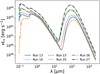 |
Fig. 3 SED prediction from the baseline analysis for the six runs analyzed in this work. |
3.4 Stellar modeling
In our framework, the dust temperature is determined via Monte Carlo simulations by propagating photon packages placed initially according to the stellar density distribution and an input stellar spectrum. To adequately model the spatial distribution of photons across the grid, we then need to provide a grid of stellar densities, as well as a corresponding global spectrum. To produce the stellar density grid, because star particles are collisionless in the SPH formulation, we interpolate them onto a regular cubic mesh (the same used for all the inputs of RADMC-3D, see Sect. 3.5) via a Cloud-In-Cell (CIC) scheme. In addition, we explicitly verified that using the SPH kernel to interpolate the stellar particles induces negligible differences compared to the results obtained with the CIC kernel. Because the simulation resolution is not high enough to resolve single stars, to generate the input spectrum we treat star particles as stellar populations and model the spectrum of each one by means of the STARBURST99 stellar population spectral synthesis code (Leitherer et al. 1999), following the approach adopted by Liang et al. (2019) to model stellar spectra in simulated galaxies at cosmic noon similar to the ones investigated herein. We ran STARBURST99 assuming the PADOVA stellar evolution tracks (see, e.g., Bressan et al. 1993; Marigo 2001; Bressan et al. 2012, and references therein) and a Kroupa (2001) IMF in the stellar mass range [0.1,100] M⊙, consistent with the setup used for the hydrodynamic simulations. Afterwards, given the age (computed as the difference between formation time and time of the snapshot under analysis), metallicity, and mass of each star particle, we interpolated these quantities onto the same spatial grid as the one introduced in Sect. 3.5. Then, we generated a synthetic spectrum per cell, interpolating within a grid of values of metallicity and age provided by the STARBURST99 simulations. Eventually, we obtained a single global spectrum for the whole grid by summing all the spectra throughout the simulation grid.
We notice that for the baryon particle mass resolution ≳105 M⊙, stellar populations that are enshrouded in their dusty clouds may need to be treated by means of specific stellar population synthesis accounting for dusty star-forming regions (see, e.g., Jonsson et al. 2010; Ma et al. 2019), such as, for instance, MAPPINGS-III (Allen et al. 2008) or TODDLERS (Kapoor et al. 2023). Nonetheless, the simulations used in this work have baryon mass particle resolution that is equal or lower than the mentioned threshold; therefore, for these cases, it is safe to use STARBURST99. However, we caution that a different approach to implementing the aforementioned libraries may be needed when postprocessing simulations with worse resolutions.
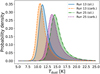 |
Fig. 4 Dust temperature probability density distribution function for the silicate (blue solid) and carbonaceous (orange dashed) dust species in run 13 and for the analogous species in run 25 (green dotted-dashed and purple dotted, respectively). |
3.5 Interpolation of particles onto grids for RADMC-3D
To perform simulations via RADMC-3D, the user must supply the input files in mesh format. To this end, we interpolated the gas particles of the simulations onto a (256, 256, 256) cell grid spanning a volume of V = (30 kpc)3 (corresponding to a physical cell resolution of l ~ 117 pc), using the 3D Wendland (1995) C2 kernel. In this way, we obtained the following mesh fields: gas density, gas velocity along the three coordinate directions, and gas metallicity. As anticipated in Sect. 3.4, the stellar density grid is obtained by means of a CIC interpolation scheme onto the same (256,256,256) mesh used for the interpolation of the other fields mentioned above (gas density, velocity, and metallicity).
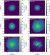 |
Fig. 5 Dust continuum luminosity images at λ = 100 µm, viewed face-on, for the six different runs analyzed in this paper, after ∆t = 0.2 Gyr from the end of the relaxation phase. The run each image refers to is reported inside the corresponding panel. |
4 Analysis, results, and discussion
In this section, we present the results obtained in each phase of the analysis and describe how we performed a comparative analysis of the different simulations investigated in this work. Throughout the work, we only considered the face-on projection of the six studied galaxies to make sure we have been to perform a fair comparison. Thus, we have left the assessment of the impact of inclination for future research. When presenting our results, we designate the radiative transfer run with the following fiducial setup as the “baseline” analysis: time snapshot at ∆t = 0.2 Gyr, with DGR following the scaling relation reported in Eq. (1), dust composition modeled as an effective mixture of silicate and carbonaceous grains with C/O = 0.8, and grain size distribution following an effective scaling n(a) ~ a−3.5. When relevant, we compared the results of our simulations; this was done for runs 13 and 25 specifically, because they represent examples of a smooth and a clumpy disc, respectively.
We tested the impact of the simulation’s resolution (number of SPH particles), as given in Appendix A.4. In fact, while the resolution is not included in our model as a parameter (and it rather represents an intrinsic property of the used simulation), it is still instructive to be aware of its impact on the predicted observables.
4.1 Dust continuum radiative transfer
The first step in our procedure consists in running the Monte Carlo radiative transfer simulations to determine the dust temperature throughout the simulation box. Then, once the cell-wise dust temperature has been computed, we can obtain the SED and mock images at arbitrary wavelength via ray tracing7.
Figure 3 shows the resulting SEDs throughout the whole probed wavelength range for the six simulations studied in this paper. Here (and in the SED plots presented in the remainder of the paper) the model for the SED is computed through radiative transfer at nλ = 150 different wavelengths, evenly spaced in log scale, throughout the probed spectral interval; this ensures a proper sampling of the SED. The shape of the SED looks similar across different simulations and it is in reasonable agreement with the SEDs of galaxies at cosmic noon8 measured from observations (e.g., Ouchi et al. 2008), as well as from simulations (e.g., Liang et al. 2019). This holds especially true if we take into account the uncertainty in our modeling, given that the hydrodynamic simulations we have considered herein do not include a built-in dust treatment, nor a self-consistent cosmological evolution. To assess the uncertainty of the DGR on the predicted SED, we computed the variance from 50 simulations, varying the parameters of Eq. (1) within the uncertainties reported by Li et al. (2019) and adopting a proper covariance matrix. The resulting uncertainty is typically of the order of one up to a few percent; hence, it is negligible compared to other sources of uncertainty and to the deviations induced by the different investigated models for the dust composition and grain size. Thus, we have not displayed these uncertainties in the SED plots for visual clarity.
Furthermore, we performed diagnostics for the resulting dust temperature and analyzed the resulting distribution. In this case, we adopted the fiducial baseline dust composition. We plot the distribution of the in-cell (i.e., not weighted by mass) dust temperatures for runs 13 and 25 in Figure 4, distinguishing between the silicate (blue solid for run 13, green dotted-dashed for run 25) and carbonaceous grains (orange dashed for run 13, purple dotted for run 25). The resulting dust temperatures display a set of consistent distribution results in all cases, within the range of 1–60 K9, and the majority of the distribution lies in the range of 10–20 K. Carbonaceous grains are found to be slightly cooler than silicate grains by a few Kelvin degrees than silicate grains. In addition, to perform a consistent comparison with metrics for the dust temperature derived from observations, we also computed the “mass-weighted” dust temperature, Tmw, and the “peak” temperature, Tpeak. Specifically, the former is computed as the cell-wise average temperature weighted by dust mass, whereas the latter corresponds to the peak temperature obtained by fitting a black body template to the infrared (IR) SED (Casey 2012; Casey et al. 2014). We obtained Tmw ~ 22.8 K and Tpeak ~ 24.1 K for run 13, along with Tmw ~ 27.4 K and Tpeak ~ 31.5 K for run 25. These values are in reasonable agreement with the detailed study of the dust temperature based on simulations of galaxies at z = 2 (e.g., Liang et al. 2019), as well as a plethora of observational results of 20 K ≲ Tpeak ≲ 40 K (see, e.g., Magnelli et al. 2014; Simpson et al. 2017; Thomson et al. 2017; Zavala et al. 2018; Schreiber et al. 2018). It is worth mentioning that the dust from run 25 is, on average, warmer than that from run 13. This fact can be explained by noticing that the UV part of the SED of run 25 (gray dashed line in Figure 3) is significantly brighter than its counterpart from run 13 (blue solid line in Figure 3), due to a higher abundance of young stellar populations emitting energetic radiation. This is in turn due to the fact that the higher gas fraction in run 25 favours disc fragmentation and star formation. Furthermore, from the fit of the modified black body model to the IR SED, we obtained values of the mean emissivity index β ~ 1.42 and β ~ 1.41 for runs 13 and 25, respectively, both broadly consistent with the value β = 1.60 ± 0.38 reported by Casey (2012) and derived from observations. We also notice that the consistency with both simulations and observations of Tpeak already represents a good consistency check that the SED of our simulations peaks at the correct wavelength.
Similarly to Liang et al. (2019), we notice that at the redshift we are assuming here (z ~ 2), the contribution to the radiation field from the cosmic microwave background is negligible (e.g., da Cunha et al. 2013); and hence, we did not include it. Also, we neglected the contribution from the external UV radiation field, whose effects will be investigated in a future work based on cosmological boxes with consistent environmental dependencies and cosmic evolution over time.
We further investigated the results of our radiative transfer computations by visually inspecting the continuum images at different IR wavelengths. In Figure 5, we show the luminosity images of the different runs at λ = 100 µm of the fiducial snapshot after ∆t = 0.2 Gyr after the end of the relaxation phase. To ease the comparison, the images share the same color scale. While the resulting morphology is qualitatively similar to that of the images in Figure 1, displaying gas mass surface density maps, the small-scale structures are brighter in the continuum images, compared to the background than in the density maps.
Furthermore, in some cases (especially runs 25 and 26), there appears to be a diffuse radiation component that extends out to large galactocentric distances. Figure 6 displays the radial luminosity profiles at λ = 100 µm for the same galaxies shown in Figure 5. This quantitatively shows that runs 25, 26, and 27 are indeed generally brighter than the other runs at fixed galactocen- tric distance. This is mostly due to the fact the these simulations were run with a higher gas fraction, which corresponds to a larger dust mass in our model and, hence, to a higher emitted IR luminosity. Figure 7 shows instead the continuum images for run 13 at λ = 0.7 µm (top left) and λ = 1.5 µm (top right) to match the median redshift of the JWST NIRCam F070W and F150W filters (Rieke et al. 2005, 2023), respectively, λ = 70 µm (mid left) and λ = 100 µm (mid right) to match Herschel PACS filters (Poglitsch et al. 2010), and λ = 250 µm (bottom left) and λ = 500 µm (bottom right) to match Herschel SPIRE filters (Griffin et al. 2010). In this case, we did not saturate the mock images to the same color scale to maximize the visual contrast, since the luminosity images span intrinsically different ranges. While the morphology is reassuringly self-similar in the PACS and SPIRE images, at shorter wavelengths (λ = 0.7 µm and λ = 1.5 µm), there appears to be a clear diffuse component extending out to the whole disc (that is not visible in others) coming from the stellar emission. This can be quantitatively seen in Figure 8, which displays the radial luminosity profiles for run 13 at the same wavelengths shown in Figure 7. In particular, at the shorter wavelengths the luminosity curve is shallower than at longer wavelengths, being fainter towards the center, but brighter towards the outskirts of the galaxy. The different slopes of the short-wavelength and long-wavelength radial luminosity profiles are due to the fact that the former are mainly due to the stellar emission, whereas the latter arise from the dust emission. As such, they mirror the spatial distribution of the stellar and dust density, respectively. Specifically, the dust emission is significantly more luminous in the central part of the galaxy, while the stellar emission has a smoother decrease in luminosity with radius.
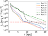 |
Fig. 6 Radial luminosity profiles at λ = 100 µm for run 13 (blue solid), run 16 (orange dashed), run 23 (purple dotted), run 25 (gray dashed), run 26 (green dotted-dashed), and run 27 (black dotted-dashed). The red dashed line marks the lower limit of the colorbar in Figure 5. |
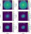 |
Fig. 7 Dust continuum luminosity images at λ = 0.7 µm (top left), λ = 1.5 µm (top right), λ = 70 µm (mid left), λ = 100 µm (mid right), λ = 250 µm (bottom left), and λ = 500 µm (bottom right), viewed face-on, for run 13, after ∆t = 0.2 Gyr from the end of the relaxation phase. |
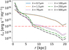 |
Fig. 8 Radial luminosity profiles for run 13 at λ = 8 µm (blue solid), λ = 24 µm (orange dashed), λ = 70 µm (purple dotted), λ = 100 µm (gray dashed), λ = 250 µm (green dotted-dashed), and λ = 500 µm (black dotted-dashed), obtained from the dust continuum luminosity maps shown in Figure 6. The red dashed line marks the lower limit of the colorbar in Figure 7. |
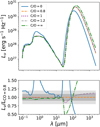 |
Fig. 9 Results from the baseline analysis for run 13 (orange dashed), compared to the results from the other studied dust compositions: C/O ~ 0 (blue solid), C/O ~ 1 (purple dotted), C/O ~ 1.2 (gray dashed), and C/O → ∞ (black dotted-dashed). Top: SED predictions as a function of the relative abundance of silicate and carbonaceous grains. Bottom: Ratios between the SED of each studied case and the baseline (C/O ~ 0.8), with the light and dark gray bands showing a 10% and 20% difference, respectively. |
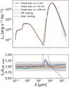 |
Fig. 10 Results from the baseline analysis for run 13 (orange dashed), compared to the results from the other studied grain size distribution results: fixed grain size with a = 1 nm (blue solid), fixed grain size with a = 10 nm (gray dashed), fixed grain size with a = 100 nm (green dotted), and explicit modeling of the grain size distribution n(a) ~ a−3.5 (purple dotted). Top: SED predictions as a function of the modeling of the grain size distribution. Bottom: Ratios between the SED of each studied case and the baseline (effective mixture of grains with a distribution of n(a) ~ a−3.5), with the light and dark gray bands showing a 10% and 20% difference, respectively. |
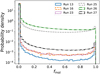 |
Fig. 11 Probability density distribution function for the molecular fraction fmol (see Sect. 3.2). All the distributions feature a major peak around fmol ~ 0 (fully atomic gas) and a less significant peak around fmol ~ 1 (fully molecular gas). The displayed curves are normalized so that they subtend an area equal to unity. |
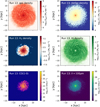 |
Fig. 12 Gas mass surface density (top left), stellar mass surface density (top-right), H2 mass surface density (mid-left), and H I mass surface density (mid-right) maps, continuum luminosity image at λ = 100 µm (bottom-left), and CO(1–0) luminosity image (bottom-right), viewed face- on, for run 13, after ∆t = 0.2 Gyr from the end of the relaxation phase. |
4.2 Model of dust composition and grain size
We address the impact of the model of dust abundance, composition, and grain size by looking at the variation in the prediction of the SED with respect to our baseline.
Figure 9 shows the comparison between the SEDs obtained assuming the five different relative silicate and carbonaceous compositions outlined in Sect. 3.1.2. The top panel shows the resulting SEDs, whereas the bottom panel displays the ratios between the SED of each studied case and that of the baseline (i.e., the case with C/O = 0.8), with the gray bands marking 10% (darker) and 20% (lighter) deviations, respectively. One easily notices that the three models with C/O = 0.8 (orange dashed), C/O = 1 (purple dotted), and C/O = 1.2 (gray dashed) have well-converged SEDs (within just a few percent deviations) at λ ≲ 10 µm, and display reasonable deviations at ~ 10–15% at λ ≳ 100 µm. On the other hand, it is interesting to notice that the cases comprising only silicate grains (C/O = 0, blue solid) and only carbonaceous grains (C/O → ∞) show larger deviations. In particular, if compared to the other cases, the peaks of the IR region of the SED are clearly displaced towards shorter wavelengths for the C/O = 0 case and towards longer wavelengths for the C/O → ∞ case, consistently with the dust grains being on average hotter and cooler, respectively.
Figure 10 shows a similar comparison to that in Figure 9, but analyzing different prescriptions for the grain size distribution. The bottom panel is again normalized by the SED predictions from the baseline analysis, which consists this time in assuming an effective scaling of the dust grain size (see Sect. 3.1.3). In particular, one finds that all the curves converge within <10% deviations with respect to the baseline analysis at λ≲10 µm, whereas they tend to have a larger dispersion at longer wavelengths (within ≲25% deviations); with the exception of the run at a fixed size of a = 100 nm, which diverges a great deal more. This indicates that while assuming a fixed size for the grains is most likely inadequate, adopting an effective scaling may be a reasonable assumption in many cases. Nonetheless, an assessment of the accuracy and the convergence of the models should be performed case by case.
4.3 Atomic-to-molecular transition
Figure 11 shows the resulting distribution for the cell-wise molecular fraction, fmol = ρH2/ρgas,tot, for the six different simulations investigated herein. In particular, in this plot fmol = 0 means fully atomic gas, whereas fmol = 1 means that the gas is fully molecular. In generating this plot, we have considered only cells with non-zero gas density and discarded all the cells devoid of gas. The displayed curves are normalized so that they subtend an area equal to unity. The resulting distributions are clearly skewed in all the studied cases and feature a major peak at fmol = 0, along with a much less significant peak at fmol = 1. This implies that the fully atomic and fully molecular gas phases are strongly and only mildly preferred, respectively, over intermediate cases featuring a mixture of the two. We also notice that this phenomenon is strongly resolution-dependent. In fact, runs 25 and 26, which have higher resolution compared to the other four simulations, display a consistently larger probability of intermediate fmol values by ≳2 order of magnitude with respect to the other cases. This result is consistent with the fact that a higher resolution allows us to better resolve regions with intermediate and high gas density conditions, where the formation of the molecular phase is favoured (see, e.g., Capelo et al. 2018). In contrast, the high-resolution run 13 does not show the same behaviour, due to its lower gas fraction, fgas = 0.3.
We will further investigate the atomic and molecular phase balance under different galaxy formation models in future works, as well as the resulting scaling relations linking them to other galaxy properties and the impact of the gas phase morphology on the star formation activity and history.
Figures 12 and 13 show a series of galaxy properties for runs 13 and 25, respectively: the gas density (top left), stellar mass density (top right), H2 mass density (mid left), H I mass density (mid right), CO(1–0) luminosity (bottom left), and continuum luminosity at λ = 100 µm (bottom right). By comparing the H I density and H2 density maps, it turns out that the molecular phase is more concentrated towards the center, while the atomic phase is spread over a more extended disc (as also found in Capelo et al. 2018). This is (at least partly) due to the gas in the central region being denser and, hence, more likely to be in the molecular phase. Also, the atomic component is found to be underdense towards the center of the galaxy with respect to the average, where the molecular phase is dominant. This fact can be appreciated more quantitatively in Figures 14 and 15, displaying the radial density profiles of the total gas density, stellar density, H2 density, and H I density, for runs 13 and 25, respectively. From the resulting curves, it is clear that the molecular component dominates the total gas density profile at the center, while the atomic component dominates towards the outer regions of the discs. This fact is consistent with z = 0 galaxy observations, wherein H I is found to form a disc, which extends out to radii ∼5–10 times larger than the optical disc (see, e.g., Walter et al. 2008), and where the CO emission often has a much smaller galactocentric extent than the optical disc (see, e.g., Leroy et al. 2008; Nagy et al. 2022).
In particular, we notice that (as anticipated) the computation of the H I distribution in the studied galaxies within our pipeline enables us to obtain predictions for the 21-cm line (amongst others), which is of paramount importance in the view of the future unprecedented observational data which will be collected by the Square Kilometre Array (SKA, Dewdney et al. 2009).
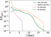 |
Fig. 14 Radial surface density profiles for run 13 of the total gas density (blue solid), stellar density (orange dashed), H2 density (purple dotted), and H I density (green dashed). The curves are normalized to the total gas density in the innermost bin (i.e., at the center). |
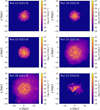 |
Fig. 16 CO(1–0) luminosity images, viewed face-on, for the six different runs analyzed in this paper, after ∆t = 0.2 Gyr from the end of the relaxation phase. The run each image refers to is reported inside the corresponding panel. |
4.4 CO line radiative transfer
Figures 12 and 13 show also the CO(1–0) luminosity images for runs 13 and 25 (bottom left), respectively. All the runs presented herein are obtained under the local thermal equilibrium (LTE) assumption. We address the impact of LTE versus non-LTE in Appendix A.2, but we anticipate that the impact is a deviation of just a few percent, which we neglect in the runs presented in this section due to their tiny contribution. In future studies, we will assess the impact of this assumption on a case-by-case basis and adopt the non-LTE computation when its deviation from LTE becomes non-negligible.
We start by noticing that the CO luminosity highlights the high-density regions of the studied galaxies (as expected from molecular gas) and, in particular, the clumpy structure of runs 25, 26, and 27 (see Figure 16, where we expand this comparison and show the CO(1–0) luminosity image for all the different runs). This is particularly important in the light of using the mock CO images to study the nature of massive clumps in high-redshift galaxies, as observed with ALMA (see Dessauges-Zavadsky et al. 2019, 2023), which will be the subject of a forthcoming publication. It is interesting to notice that runs 25 and 26 (which were run at high resolution and have a gas fraction fgas = 0.5) display a pronounced diffuse CO radiation in the outskirts of the disc. In contrast, run 27 does not display an analogous diffuse component despite having been run with the same gas fraction (fgas = 0.5) as runs 25 and 26. A careful investigation of this fact revealed that the violent fragmentation that the disc undergoes starts from the inner regions of the disc; at the time snapshot studied herein (∆t = 0.2 Gyr from the end of the relaxation phase) the molecular gas has formed preferentially towards the center. For this reason, we do not observe a diffuse CO component in run 27 at the investigated snapshot. In contrast, we explicitly verified that, at later times, run 27 builds up a molecular gas radial profile extending out to larger galacto- centric distances, and shows a consistent CO diffuse component. This is due to the fact that, because run 27 was run at lower halo concentration than runs 25 and 26 (c = 6 for run 27, c = 10 for runs 25 and 26), the rotation velocity at the same galactocentric distance is lower and the orbital time longer in the disc of run 27 than in the discs of runs 25 and 26, which is consistent with a delayed evolution in run 27. We will study this phenomenon more in detail in a forthcoming paper addressing the nature of the giant clumps observed in CO maps.
We also quantify the relative emission of rotational lines at higher quantum rotational number with respect to the CO(1–0) transition. This is shown in Figure 17, where we display the luminosity ratio LCO((J+1)–J) LCO(1–0) for different quantum numbers J – known as the CO spectral line energy distribution (SLED) – and for all the runs studied herein. We also report in the same plot the observational results for the CO SLED from cosmic noon galaxies (Bothwell et al. 2013; Spilker et al. 2014; Daddi et al. 2015; Boogaard et al. 2020). We notice that the predicted curves from our model are in reasonable agreement with the observed galaxies and well within the scatter of the observed CO SLED for galaxies at 1.5 < z < 3.5 (see also, e.g., Vallini et al. 2018). The only galaxy with higher CO SLED than the rest of the sample is run 27, consistently with the fact that disc fragmentation and, hence, molecular gas formation, are favored due to the large gas fraction.
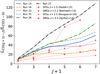 |
Fig. 17 CO SLED for the baseline analysis of the six simulations studied in this work, after ∆t = 0.2 Gyr from the end of the relaxation phase. The thin red lines display the literature results for different galaxies at cosmic noon. |
5 Time evolution
As an additional application of the framework presented in this paper, we study the evolution over cosmic time of two simulations of our sample, namely, runs 13 and 25. In particular, we analyze the predicted observables for these two galaxies at four different timesteps: ∆t = 0.1, 0.2, 0.5, and 0.8 Gyr after the end of the relaxation phase. Figures 18 and 19 show the gas surface density maps for runs 13 and 25, respectively, at the four aforementioned cosmic times. By performing a visual inspection, we can easily notice how the disc evolves over time in both cases, acquiring a more and more structured morphology the later the time. While run 13 develops a stable spiral structure after ∆t = 0.8 Gyr, run 25 undergoes a quicker gas depletion and by the same time the galaxy has largely devoided its gas reservoirs due to an intense star formation activity driven by a larger gas fraction than in run 13 (Tamburello et al. 2015). In addition, the disc in run 25 develops a pronounced clumpy structure, while run 13 does not. This is due to the higher gas fraction in run 25, which favours disc fragmentation (see Tamburello et al. 2015).
Figures 20 and 21 display the predicted SED for runs 13 and 25, respectively, following a similar structure as that of Figure 9. In particular, the bottom panel is this time normalized to the SED computed at ∆t = 0.2 Gyr (i.e., the snapshot analyzed throughout this work) to perform a meaningful comparison with the results presented in the remainder of this paper. Both runs 13 and 25 feature a monotonic temporal evolution of the UV region of the SED, with the both the UV and FIR emission becoming fainter with time. This is consistent with the presence of older stellar population and lower dust density (the latter due to the fact that the dust density is proportional to the gas density in our model) and that the gas gets depleted by star formation and there is no external gas accretion in our simulations, respectively. We argue that there may be a significant dependence on the variation of the predicted SED when clumps are formed and disrupted, which we will investigate in a forthcoming paper. We also caution that this result applies in the case of the studied simulations, which are isolated discs, but they may not represent a realistic scenario in cosmological simulations that include gas accretion onto galaxies.
Finally, Figure 22 shows the evolution over time of the total CO(1–0) luminosity for runs 13 (blue solid) and run 25 (orange dashed), respectively, normalized to the CO(1–0) luminosity computed after ∆t = 0.2 Gyr (i.e., the baseline analysis). The resulting curves highlight that the CO(1–0) luminosity increases over time in run 13, reaching a maximum at ∆t = 0.5 Gyr, and then decreases towards later time. This hints towards the fact that this galaxy undergoes a first phase of molecular cloud formation, which favours the CO emission, while after ∆t = 0.5 Gyr gas depletion due to star formation and feedback starts to dominate causing a decrease of CO luminosity. On the contrary, the evolution of run 25 is different, as the CO luminosity decreases monotonically over time. This fact is consistent with the point made earlier in this work, namely, the galaxy disc evolved much more quickly and depletes the gas more efficiently (possibly because of clump formation) than what occurs in run 13.
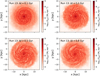 |
Fig. 18 Gas mass surface density maps, viewed face-on, for run 13, after ∆t = 0.1 Gyr (top left), ∆t = 0.2 Gyr (top right), ∆t = 0.5 Gyr (bottom left), and ∆t = 0.8 Gyr (bottom right) from the end of the relaxation phase, respectively. |
6 Summary and conclusions
This work presents the implementation and validation of an end-to-end pipeline (dubbed RTGen) based on the RADMC-3D code (Dullemond et al. 2012) aimed at performing a posteriori continuum and spectral line radiative transfer simulations of hydrodynamic simulations of galaxies. We summarize the main steps and features of the pipeline, as well as the main results and conclusions below.
The implemented framework relies on a Monte Carlo radiative transfer algorithm that first determines the dust temperature and then ray-traces photons at a given wavelength, solving for the continuum or line transfer equation, depending on the requested setup. Given that RADMC-3D is model-agnostic and only runs the radiative transfer computation once the physical problem is fully specified, the pipeline implements a detailed modeling of the gas, dust, and stellar density leveraging state-of-the-art public tools, models, and observational results from the literature. In particular, we first interpolate the gas and star particles onto a grid using an SPH kernel and a CIC scheme, respectively. Afterwards, we model the input stellar spectrum for each of the studied galaxies as sum of the spectra of the different stellar particles, computed by relying on the STARBURST99 stellar population synthesis code (Leitherer et al. 1999). Since the dust formation, growth, and destruction are not tracked in the hydrodynamic simulations used in this paper, we predict the dust abundance from the gas density field by applying a scaling relation linking the DGR to the gas metallicity, measured from the SIMBA simulation and found to agree well with state-of-the-art observational results (Li et al. 2019). After running the Monte Carlo dust radiative transfer and the ray tracing to obtain continuum images, we obtained the radiation field self-consistently in our pipeline from radiative transfer at λ = 0.1 µm and used it to compute the atomic-to-molecular transition presented in Gnedin & Kravtsov (2011). We then calibrated it onto a high-resolution hydrodynamic simulation. This allowed us to obtain predictions for the atomic (H I) and molecular (H2) density. Eventually, we used the latter to compute the CO abundance and predict the CO luminosity via line radiative transfer computation.
Within our dust modeling, we tested the assumptions behind dust composition and grain size. In particular, we found that assuming dust composition of approximately similar proportion of silicate and carbonaceous grains yields a reasonable convergence in the predicted SEDs, while we observe significant deviations when the dust is assumed to be composed just by silicate grains. When looking into the results from different models for the dust grain size, we find a good convergence (within <10% deviations) of the predicted SEDs at λ ≲ 10 µm for all the studied cases, whereas the SEDs tend to diverge at longer wavelengths. This suggests the need for a careful study and testing of the adopted model on a case-by-case basis.
The atomic and molecular splitting yields a skewed distribution for the molecular fraction, fmol, which is found to have a strong dependence on resolution and on the gas fraction. In addition, the predicted spatial distribution with galactocentric distance of H I and H2 is in good qualitative agreement with well-studied cases in the local Universe, where the latter is found to be confined in a small disc at the center of the galaxy, whereas the former forms a disc which extends out to much larger radii (e.g., Walter et al. 2008; Leroy et al. 2008).
Eventually, we predict the CO luminosity by calibrating the H2-to-CO abundance and forward-modeling the radiative transfer, assuming the Milky Way CO-to-H2 conversion factor αCO (e.g., Bolatto et al. 2013). The predicted CO luminosity images show greatly enhanced morphological structure in the galaxies and, in particular, they highlight the clumpy structure that will be the subject of a more detailed investigation in a forthcoming paper.
We note that while we have thoroughly addressed the impact of the dust modeling, we will perform a systematic investigation of the uncertainties associated with the atomic-to-molecular transition and on the H2-to-CO conversion in a future work.
We envision that this pipeline can be used for a variety of studies of galaxy formation and evolution, allowing us to study the impact of several different aspects of galaxy formation and feedback models on typical galaxy observables such as the SEDs and multi-wavelength images. In particular, the mock images produced within the RTGen pipeline can be postprocessed by applying JWST filters to continuum images and ALMA systematics (array configuration and noise, among others) to CO images using CASA (CASA Team 2022). In a forthcoming publication, we will use these techniques to perform a comparative study of the nature of massive clumps in high-redshift galaxies, as was done by Tamburello et al. (2017) leveraging the Hα line.
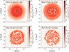 |
Fig. 19 Gas mass surface density maps, viewed face-on, for run 25, after ∆t = 0.1 Gyr (top left), ∆t = 0.2 Gyr (top right), ∆t = 0.5 Gyr (bottom left), and ∆t = 0.8 Gyr (bottom right) from the end of the relaxation phase, respectively. |
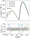 |
Fig. 20 Top: Comparison of the SED predictions for run 13 at different time snapshots, ∆t = 0.1 Gyr (blue solid), ∆t = 0.2 Gyr (orange dashed), ∆t = 0.5 Gyr (purple dotted), and ∆t = 0.8 Gyr (green dotted- dashed) after the end of the relaxation phase, respectively. Bottom: Ratios between the SED of each studied case and the baseline (∆t = 0.2 Gyr). |
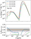 |
Fig. 21 Top: Comparison of the SED predictions for run 25 at different time snapshots, ∆t = 0.1 Gyr (blue solid), ∆t = 0.2 Gyr (orange dashed), ∆t = 0.5 Gyr (purple dotted), and ∆t = 0.8 Gyr (green dotted- dashed) after the end of the relaxation phase, respectively. Bottom: Ratios between the SED of each studied case and the baseline (∆t = 0.2 Gyr). |
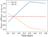 |
Fig. 22 Total CO(1–0) luminosity at different time snapshots normalized to the total CO(1-0) luminosity ∆t = 0.2 Gyr after the relaxation phase, for run 13 (blue solid) and run 25 (orange dashed). The red dotted-dashed line marks unity ratios. |
Data availability
The code implementing the models presented in this work is publicly available10.
Acknowledgements
The authors warmly thank the anonymous referee, whose insightful comments helped improving the quality of the manuscript. The authors wish to also acknowledge Cornelis Dullemond – the author of the RADMC-3D code – for making the code available and for assistance on the usage of the software. FS acknowledges the support of the Swiss National Science Foundation (SNSF) 200021_214990/1 grant. FS is also grateful to Dr Gaia Lacedelli, for availability of computing resources. LM acknowledges support from the SNSF under the Grant 200020_207406. PRC acknowledges support from the SNSF under the Sinergia Grant CRSII5_213497 (GW-Learn).
Appendix A Monte Carlo radiative transfer in RADMC-3D
In this appendix, we summarize the main working principle behind the RADMC-3D code, as well as that of the Monte Carlo radiative transfer implemented therein.
Dust temperature computation
RADMC-3D implements the radiative transfer Monte Carlo method described in Bjorkman & Wood (2001), including the continuous absorption method (Lucy 1999).
The whole method is based on enforcing radiative equilibrium, for which the absorbed energy in a volume element (in our case, a cell of the grid) must be re-radiated.
We can express the energy emitted over a time interval ∆t as
 (A.1)
(A.1)
where jv = ρLvBv(T) is the dust thermal emissivity, ρ is the dust density, Lν is the dust absorption opacity, Bν(T) is the Planck function at temperature T, kp(T) = LνBνdυ/B is the Planck mean opacity, and B = σT4/π is the Planck function integrated over frequency, which is the result of the Stefan-Boltzmann law with σ the Stefan-Boltzmann constant.
Briefly, RADMC-3D injects in the grid a given number of photon packages Nγ (which is an input parameter), each package with the same initial energy Eγ = E/Nγ, where E is the total energy in the model. In our framework, because the source of luminosity in our radiative transfer simulations is a stellar density grid (in contrast to single stars, as the code allows in other configurations), the energy of each photon package is computed using the total luminosity in a cell, instead of that of a single star.
After this step, each photon package in RADMC-3D is assigned a random frequency sampled from the chosen SED. In this way, the number of photons constituting the photon package will be automatically determined by energy conservation. We describe the modeling of stellar sources and the associated SED in Sect. 3.4.
Once a photon package has been initialized, its motion is started in a random direction. At this point, a random number z is obtained via a uniform random sampling from the interval I = [0, 1). In this formalism, the mean free path of a photon package between two events is assumed to be x = − ln(z), which corresponds to a physical displacement l = x/[ρ(Lν + σν)], where σν is the dust scattering opacity (Lucy 1999). After displacing each photon package by l along the initial direction, if the package goes beyond the boundary of the initial cell, then one computes l again. If instead a photon package remains inside the same cell, it gets scattered by a dust grain if z < σν/(Lν + σν), or it gets absorbed otherwise.
When a photon package gets scattered, the frequency is kept unchanged, while only the direction is reassigned, depending on the scattering approximation used. RADMC-3D implements isotropic scattering, as well anisotropic scattering in different degrees of complexity and realism. The different scattering mechanisms are described in Sect. A.3.
When a photon package gets absorbed, it must be re-radiated instead. In this case, both the direction and the frequency must be reassigned. Assuming LTE, the emitted energy after an absorption event is given by the radiative equilibrium condition expressed in Eq. A.1.
Each time a photon package enters a cell, the energy associated with the cell increases and the dust temperature must be recomputed. This treatment is different from that in Bjorkman & Wood (2001), in which the temperature is recomputed only if an absorption event occurs. Hence, in RADMC-3D the energy increase in each cell is given by the energy Eγ associated with the photon package. Enforcing the radiative equilibrium condition and setting Eem = Eγ gives an implicit equation for the dust temperature, which must be solved iteratively at each step.
In this way, a photon package travels throughout the probed volume until it escapes, at which point a new package is launched and the simulation continues until all photons have been injected into the box and they have escaped it. We notice from now that the calculation will be subject to the number of photon packages used in the calculation, given the intrinsic degree of stochasticity. In general, one expects that the higher the number of photons, the less prone the results will be to stochastic fluctuations, but the more expensive a Monte Carlo will become. In Sect. A.5, we show that the computation converges to sub-percent deviations accuracy if a sufficiently large number of photon packages is chosen, and we will adopt the minimum number of packages which ensures convergence throughout this work. We refer to Lucy (1999) and Bjorkman & Wood (2001) for a more detailed treatment of the Monte Carlo radiative transfer method used herein.
A.1 Continuum transfer
Once the dust temperature has been determined using the Monte Carlo method described in Sect. A, RADMC-3D performs the raytracing of individual photons at an arbitrary wavelength defined by the user. In particular, given a photon of frequency ν, the code solves the radiative transfer equation,
 (A.2)
(A.2)
where τν denotes the optical depth at a frequency, ν. Also, Iν is the intensity of the local radiation field and αν is the extinction coefficient. In the present case, the emissivity has both a thermal emission and a scattering term:  . The thermal part,
  , is given by product of the absorption extinction
  and the Planck function. The scattering term can instead be expressed as
 (A.3)
(A.3)
where,  is the scattering extinction and
  is the scattering source function, which will be discussed more in detail in Sect. A.3.
Similarly, also the extinction term of Eq. A.2 can be expressed as the sum of two components, namely a scattering and an absorption part. In particular, one can write  , where the two addends are defined as above.
The equation is fully specified if the dust temperature, T, the dust density, ρ, the opacities, kν, and the scattering phase functions are known. In this case, we notice that T is the outcome of the Monte Carlo thermal run described in Sect. A, ρ is an input of the model, the scattering phase function is either known analytically or is pre-tabulated, and the kν coefficients are also pre-computed using Mie theory (see Sect. A.3). Hence, the equation can be readily solved at this point.
A.2 Spectral line transfer
After employing the Monte Carlo run to obtain the dust temperature, RADMC-3D can also solve the radiative transfer equation (Eq. A.2) for spectral lines. Given a spectral line arising from a transition between two energy levels i and j, Eq. A.2 reads
 (A.4)
(A.4)
with
 (A.5)
(A.5)
where N is the total number density of the studied atom/molecule, ni is the relative abundance of the atom/molecule at level i, Aij is the Einstein coefficient for the emission from level i and j, Bij and Bji are the Einstein B-coefficients, and  is the line profile function. Here, N, Aij , and bij are supplied by the user as inputs, while ni and
  are computed internally within the code. We refer to the documentation of RADMC-3D for a complete description of the implementation, which goes beyond the scope of this paper.
RADMC-3D implements the solution of the radiative transfer equation in LTE conditions, as well as the approximated solution in non-LTE conditions with different methods. We notice that a full non-LTE treatment for line transfer is not available in RADMC-3D (see, instead, e.g., Matsumoto et al. 2023, for a self-consistent treatment of dust and non-LTE CO radiative transfer), but for most of the cases it would probably become too computationally expensive and probably not necessary. In this work, we test the large velocity gradient (hereafter LVG, also known as Sobolov approximation) + Escape Probability (hereafter, EscProb) non-LTE method (Ossenkopf 1997; Shetty et al. 2011). In this method, the local mean intensity J = (1 − β) S is integrated over the line, where S is the line intensity and β is the escape fraction parametrized as β = (1 − exp(−τ))/τ, where τ = min(τLVG, τEscProb): in this formalism, one seeks to determine the minimum optical depth which causes a photon to escape due to either the presence of large velocity gradients (τLVG) or due to the finite width of the line (τEscProb). In the LVG method, τLVG ∝ 1/|∇υ| (see, e.g., van der Tak et al. 2007; Shetty et al. 2011), where ∇υ is the gradient of the local velocity field, such that the escape probability is larger than the absolute value of the velocity gradient. In the escape probability method, τEscProb ∝ L/wline, where L is a free scale parameter (to be supplied by the user) and wline is the width of the spectral line, where again the smaller is L the more non-local is the method becomes and for L → ∞ the case is equivalent to pure LVG.
To address the impact of assuming a simpler LTE formalism over performing the non-LTE computation, we study the CO(1–0) resulting spectra from such two methods. The results are shown in Figure A.1, where we show the spectra in the top panel, and the ratio between the non-LTE and the LTE spectra in the bottom panel. The ratios clearly show that the difference between the LTE and non-LTE computation is ≲1% across the whole spectrum. This means that, in this specific problem and under the studied configuration, the adoption of a non-LTE method is not crucial, and goes at the expense of a significantly longer computing time.
A.3 Opacity computation and scattering treatment
The scattering and absorption opacity must be computed given the features of the dust grains in the model. While the opacity is not directly computed inside RADMC-3D, we have included in the RTGen pipeline an external package to compute the opacity as a function of wavelength.11
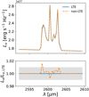 |
Fig. A.1 CO(1–0) line spectra for run 13, obtained projecting the galaxy edge-on. The top panel shows the comparison between the spectrum obtained in LTE approximation (blue solid) and the one obtained adopting the non-LTE method (orange dashed). The bottom panel displays the wavelength-wise ratio between the spectra, highlighting that the difference is ≲1% in almost all bins. |
Briefly, the opacity computation relies on Mie scattering theory (Mie 1908; van de Hulst 1958; Bohren & Huffman 1983). Following Bohren & Huffman (1983) and expressing the dust absorption opacity as kν = sνn/ρ, where sν is the interaction cross section, and n and ρ are the number and mass density of the dust respectively, one can express the total and the scattering cross sections σtot and σsc in terms of vector spherical harmonics expansion as
 (A.6)
(A.6)
 (A.7)
(A.7)
where ai and bi are the scattering coefficients, defined as
 (A.8)
(A.8)
 (A.9)
(A.9)
where ψi and ξi are the Riccati-Bessel functions, m is the complex refractive index of the considered medium, and x = 2πa/λ is the ratio between the size of the particle a and the wavelength λ.
In this way, the used piece of software allows us to obtain the scattering and absorption opacity. Also, while an exhaustive treatment of this topic goes beyond the scope of the paper (see Bohren & Huffman 1983, and references therein, for a detailed explanation), the same code also returns the scattering Müller matrix 𝒵 transforming an input Stokes vector S0 = (I0, Q0, U0, V0) into the output Stokes vector S = (I, Q, U, V) via the relation S = 𝒵S0 . For randomly-oriented particles, 𝒵 is a symmetric matrix, for which only 6 elements (e.g., the upper triangular part including the diagonal) are independent. Also, the elements of 𝒵 will depend on the angle between the incoming and outgoing scattering directions θ and on the wavelength λ. Therefore, it is necessary to compute that Müller matrix for a grid on θ and for all the λ included in the model.
With these ingredients, RADMC-3D implements six treatments of scattering, of increasing realism and complexity:
no scattering: scattering is not included. This option is clearly not realistic, but it is still instructive to test it and compare it with other ways of treating scattering;
-
isotropic scattering: in this case, the scattering source function
 in Eq. A.3 is the integral over the solid angle of the intensity Iv:
 (A.10)
which is independent of the direction;
-
anisotropic scattering with the Henyey-Greenstein phase fuction: in the anisotropic scattering case, the scattering source function can be obtained by updating the previous expression with the introduction of the scattering phase function Φ(nin, nout), which depends on incoming and outgoing direction, parametrized through the unit vectors nin and nout . Defining θ as the angle subtended by nin and nout and cos θ = µ = nin · nout, we can express Φ(nin, nout) = Φ(µ) and write the scattering source function as
 (A.11)
In this option, the scattering phase function is assumed to be the Henyey-Greenstein function (e.g., Henyey & Greenstein 1941; Toublanc 1996):
 (A.12)
where g is the anisotropy parameter and is computed numerically from Mie theory.
anisotropic scattering with the phase function tabulated by the user: in this case, one has to specify the 𝒵11 element of the Müller matrix, which is then linked to the phase function as Φ(µ) = 4π𝒵11/σ;
anisotropic scattering using the full scattering matrix for polarization and randomly-oriented particles: in this case, the full Müller matrix is used to compute the phase function, but it is still a symmetric matrix with just six independent elements;
anisotropic scattering with full polarization treatment: in this case, the potential alignment of non-spherical dust grains is taken into account and the full Müller matrix (with 16 independent elements) is used in the computation.
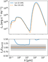 |
Fig. A.2 Results from the baseline analysis for run 16 (orange dashed) and run 22 (blue solid). Top: SED predictions as a function of the simulation’s resolution (number of SPH particles). Bottom: ratios between the SED of each studied case and the baseline, with the light and dark gray bands showing a 10% and 20% difference, respectively. |
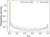 |
Fig. A.3 Same as Figure 11, but for runs 22 and 16, i.e., as a function of the simulations resolution (number of SPH particles). |
We notice that, since we are not interested in studying polarization at this stage, we do not investigate the three last options, which are also the most computationally expensive. We leave such a study for future work.
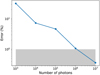 |
Fig. A.4 Maximum percentage uncertainty on the SED as a function of the number of photons used in the Monte Carlo dust radiative transfer simulations. Sub-percent convergence is reached for nphot = 107 . |
A.4 Impact of resolution
In this section, we study the impact of the simulation’s resolution on the predicted observables. In particular, we consider the high-resolution simulation counterpart of run 16 – i.e., run 22 from Tamburello et al. (2015) – and run our pipeline over it. Figure A.2 shows the comparison between the SEDs obtained from run 16 (low resolution, orange dashed) and run 22 (high resolution, blue solid). The top panel shows the resulting SEDs, whereas the bottom panel displays the ratios between the SED of each studied case and that of run 16, with the gray bands marking 10% (darker) and 20% (lighter) deviations, respectively. One clearly sees that the high-resolution case predicts a brighter SED across all wavelengths. Figure A.3 displays the resulting distribution for the cell-wise molecular fraction fmol = ρH2/ρgas,tot, similarly to Figure 11, but for runs 16 and 22. This plot shows that run 22 has generally a larger molecular fraction than that of run 16. These results can be easily understood by noticing that a higher resolution implies the formation of higher-density regions in the simulation, thereby favouring the molecular cloud formation and consequently star formation. This translates into having in such regions, on average, younger stellar populations, as well as larger dust density, given that the latter is proportional to the gas density in our framework. These two facts motivate the SED of run 22 being brighter than that of run 16 in the UV/optical regions and in the FIR region, respectively.
A.5 Convergence tests against number of photons
To study the impact of stochastic fluctuations due to the intrinsic Monte Carlo nature of our simulations and the consequent robustness of our results, we perform convergence tests studying the variation in the SED as a function of the number of photons used in our runs. In particular, the goal is to establish the minimum number of photons for which the simulations are well converged, to strike a balance between the computational cost and the stability of the results. To do so, we vary the number of photons in the range nphot = 103–107 (one case per order of magnitude, i.e., five cases in total) and run 50 dust continuum transfer simulations for each case. Afterwards, we compute the average  and SED for all the simulations of the same case and its standard deviation σ(λ), and quantify the percentage error as
  . We then compute the maximum error over the wavelength range, to have a conservative estimate of the stochastic uncertainty. Figure A.4 shows the results of this test. Our findings evidence that the maximum error in the SED is ~30% for nphot = 103, it approaches ~1% for nphot = 106, and it is ~0.1% for nphot = 107. Therefore, for all the simulations discussed in the remainder of the paper, we set nphot = 107 , to be sure to have a sub-percent convergence even in extreme cases (a 5σ deviation from the mean would correspond to a ~0.5% error).
References
- Allen, M. G., Groves, B. A., Dopita, M. A., Sutherland, R. S., & Kewley, L. J. 2008, ApJS, 178, 20 [Google Scholar]
- Aoyama, S., Hou, K.-C., Shimizu, I., et al. 2017, MNRAS, 466, 105 [NASA ADS] [CrossRef] [Google Scholar]
- Baes, M., & Camps, P. 2015, Astron. Comput., 12, 33 [NASA ADS] [CrossRef] [Google Scholar]
- Bekki, K. 2015, MNRAS, 449, 1625 [Google Scholar]
- Bialy, S., Burkhart, B., & Sternberg, A. 2017, ApJ, 843, 92 [NASA ADS] [CrossRef] [Google Scholar]
- Bjorkman, J. E., & Wood, K. 2001, ApJ, 554, 615 [NASA ADS] [CrossRef] [Google Scholar]
- Blitz, L., & Rosolowsky, E. 2004, ApJ, 612, L29 [NASA ADS] [CrossRef] [Google Scholar]
- Blitz, L., & Rosolowsky, E. 2006, ApJ, 650, 933 [NASA ADS] [CrossRef] [Google Scholar]
- Bohren, C. F., & Huffman, D. R. 1983, Absorption and scattering of light by small particles, Research supported by the University of Arizona and Institute of Occupational and Environmental Health (New York: Wiley-Interscience), 541 [Google Scholar]
- Bolatto, A. D., Wolfire, M., & Leroy, A. K. 2013, ARA&A, 51, 207 [CrossRef] [Google Scholar]
- Boogaard, L. A., van der Werf, P., Weiss, A., et al. 2020, ApJ, 902, 109 [NASA ADS] [CrossRef] [Google Scholar]
- Bothwell, M. S., Smail, I., Chapman, S. C., et al. 2013, MNRAS, 429, 3047 [Google Scholar]
- Bressan, A., Fagotto, F., Bertelli, G., & Chiosi, C. 1993, A&AS, 100, 647 [NASA ADS] [Google Scholar]
- Bressan, A., Marigo, P., Girardi, L., et al. 2012, MNRAS, 427, 127 [NASA ADS] [CrossRef] [Google Scholar]
- Bullock, J. S., Kolatt, T. S., Sigad, Y., et al. 2001, MNRAS, 321, 559 [Google Scholar]
- Camps, P., & Baes, M. 2015, Astron. Comput., 9, 20 [Google Scholar]
- Camps, P., & Baes, M. 2020, Astron. Comput., 31, 100381 [NASA ADS] [CrossRef] [Google Scholar]
- Capelo, P. R., Bovino, S., Lupi, A., Schleicher, D. R. G., & Grassi, T. 2018, MNRAS, 475, 3283 [NASA ADS] [CrossRef] [Google Scholar]
- CASA Team (Bean, B., et al.) 2022, PASP, 134, 114501 [NASA ADS] [CrossRef] [Google Scholar]
- Casey, C. M. 2012, MNRAS, 425, 3094 [Google Scholar]
- Casey, C. M., Narayanan, D., & Cooray, A. 2014, Phys. Rep., 541, 45 [Google Scholar]
- Crain, R. A., & van de Voort, F. 2023, ARA&A, 61, 473 [NASA ADS] [CrossRef] [Google Scholar]
- da Cunha, E., Groves, B., Walter, F., et al. 2013, ApJ, 766, 13 [Google Scholar]
- Daddi, E., Dannerbauer, H., Liu, D., et al. 2015, A&A, 577, A46 [NASA ADS] [CrossRef] [EDP Sciences] [Google Scholar]
- Davé, R., Thompson, R., & Hopkins, P. F. 2016, MNRAS, 462, 3265 [Google Scholar]
- Davé, R., Anglés-Alcázar, D., Narayanan, D., et al. 2019, MNRAS, 486, 2827 [Google Scholar]
- De Vis, P., Jones, A., Viaene, S., et al. 2019, A&A, 623, A5 [NASA ADS] [CrossRef] [EDP Sciences] [Google Scholar]
- Dell’Agli, F., Tosi, S., Kamath, D., et al. 2023, MNRAS, 526, 5386 [CrossRef] [Google Scholar]
- den Brok, J. S., Bigiel, F., Chastenet, J., et al. 2023, A&A, 676, A93 [NASA ADS] [CrossRef] [EDP Sciences] [Google Scholar]
- Dessauges-Zavadsky, M., Zamojski, M., Schaerer, D., et al. 2015, A&A, 577, A50 [NASA ADS] [CrossRef] [EDP Sciences] [Google Scholar]
- Dessauges-Zavadsky, M., Richard, J., Combes, F., et al. 2019, Nat. Astron., 3, 1115 [NASA ADS] [CrossRef] [Google Scholar]
- Dessauges-Zavadsky, M., Richard, J., Combes, F., et al. 2023, MNRAS, 519, 6222 [NASA ADS] [CrossRef] [Google Scholar]
- Dewdney, P. E., Hall, P. J., Schilizzi, R. T., & Lazio, T. J. L. W. 2009, IEEE Proc., 97, 1482 [Google Scholar]
- Diemer, B., Stevens, A. R. H., Forbes, J. C., et al. 2018, ApJS, 238, 33 [NASA ADS] [CrossRef] [Google Scholar]
- Draine, B. T. 1978, ApJS, 36, 595 [Google Scholar]
- Draine, B. T. 2003, ARA&A, 41, 241 [NASA ADS] [CrossRef] [Google Scholar]
- Draine, B. T., & Lee, H. M. 1984, ApJ, 285, 89 [NASA ADS] [CrossRef] [Google Scholar]
- Draine, B. T., & Bertoldi, F. 1996, ApJ, 468, 269 [Google Scholar]
- Dubois, Y., Rodríguez Montero, F., Guerra, C., et al. 2024, A&A, 687, A240 [NASA ADS] [CrossRef] [EDP Sciences] [Google Scholar]
- Dullemond, C. P., Juhasz, A., Pohl, A., et al. 2012, RADMC-3D: A multipurpose radiative transfer tool, Astrophysics Source Code Library [record ascl:1202.015] [Google Scholar]
- Esmerian, C. J., & Gnedin, N. Y. 2022, ApJ, 940, 74 [NASA ADS] [CrossRef] [Google Scholar]
- Feldmann, R., & Mayer, L. 2015, MNRAS, 446, 1939 [Google Scholar]
- Ferland, G. J., Korista, K. T., Verner, D. A., et al. 1998, PASP, 110, 761 [Google Scholar]
- Ferland, G. J., Chatzikos, M., Guzmán, F., et al. 2017, Rev. Mexicana Astron. Astrofis., 53, 385 [Google Scholar]
- Ferrarotti, A. S., & Gail, H. P. 2006, A&A, 447, 553 [CrossRef] [EDP Sciences] [Google Scholar]
- Fiacconi, D., Feldmann, R., & Mayer, L. 2015, MNRAS, 446, 1957 [Google Scholar]
- Gall, C., & Hjorth, J. 2018, ApJ, 868, 62 [CrossRef] [Google Scholar]
- Gardner, J. P., Mather, J. C., Clampin, M., et al. 2006, Space Sci. Rev., 123, 485 [Google Scholar]
- Gebek, A., Baes, M., Diemer, B., et al. 2023, MNRAS, 521, 5645 [NASA ADS] [CrossRef] [Google Scholar]
- Gnedin, N. Y., & Abel, T. 2001, New A, 6, 437 [NASA ADS] [CrossRef] [Google Scholar]
- Gnedin, N. Y., & Kravtsov, A. V. 2010, ApJ, 714, 287 [NASA ADS] [CrossRef] [Google Scholar]
- Gnedin, N. Y., & Kravtsov, A. V. 2011, ApJ, 728, 88 [NASA ADS] [CrossRef] [Google Scholar]
- Gnedin, N. Y., & Draine, B. T. 2014, ApJ, 795, 37 [Google Scholar]
- Gnedin, N. Y., Kravtsov, A. V., & Chen, H.-W. 2008, ApJ, 672, 765 [Google Scholar]
- Gnedin, N. Y., Tassis, K., & Kravtsov, A. V. 2009, ApJ, 697, 55 [NASA ADS] [CrossRef] [Google Scholar]
- Goldman, S. R., Boyer, M. L., Dalcanton, J., et al. 2022, ApJS, 259, 41 [NASA ADS] [CrossRef] [Google Scholar]
- Griffin, M. J., Abergel, A., Abreu, A., et al. 2010, A&A, 518, L3 [EDP Sciences] [Google Scholar]
- Henyey, L. G., & Greenstein, J. L. 1941, ApJ, 93, 70 [Google Scholar]
- Hernquist, L. 1993, ApJS, 86, 389 [NASA ADS] [CrossRef] [Google Scholar]
- Hirashita, H. 2015, MNRAS, 447, 2937 [NASA ADS] [CrossRef] [Google Scholar]
- Hirashita, H., & Kobayashi, H. 2013, Earth Planets Space, 65, 1083 [NASA ADS] [CrossRef] [Google Scholar]
- Hopkins, P. F., & Lee, H. 2016, MNRAS, 456, 4174 [Google Scholar]
- Jones, A. P., Köhler, M., Ysard, N., Bocchio, M., & Verstraete, L. 2017, A&A, 602, A46 [NASA ADS] [CrossRef] [EDP Sciences] [Google Scholar]
- Jonsson, P., Groves, B. A., & Cox, T. J. 2010, MNRAS, 403, 17 [NASA ADS] [CrossRef] [Google Scholar]
- Kannan, R., Garaldi, E., Smith, A., et al. 2022, MNRAS, 511, 4005 [NASA ADS] [CrossRef] [Google Scholar]
- Kapoor, A. U., Baes, M., van der Wel, A., et al. 2023, MNRAS, 526, 3871 [NASA ADS] [CrossRef] [Google Scholar]
- Khatri, P., Porciani, C., Romano-Díaz, E., Seifried, D., & Schäbe, A. 2024, A&A, 688, A194 [NASA ADS] [CrossRef] [EDP Sciences] [Google Scholar]
- Kroupa, P. 2001, MNRAS, 322, 231 [NASA ADS] [CrossRef] [Google Scholar]
- Krumholz, M. R. 2013, MNRAS, 436, 2747 [CrossRef] [Google Scholar]
- Krumholz, M. R. 2014, MNRAS, 437, 1662 [NASA ADS] [CrossRef] [Google Scholar]
- Leitherer, C., Schaerer, D., Goldader, J. D., et al. 1999, ApJS, 123, 3 [Google Scholar]
- Leroy, A. K., Walter, F., Brinks, E., et al. 2008, AJ, 136, 2782 [Google Scholar]
- Li, Q., Narayanan, D., & Davé, R. 2019, MNRAS, 490, 1425 [CrossRef] [Google Scholar]
- Li, Y., Gu, M. F., Yajima, H., Zhu, Q., & Maji, M. 2020, MNRAS, 494, 1919 [NASA ADS] [CrossRef] [Google Scholar]
- Liang, L., Feldmann, R., Kereš, D., et al. 2019, MNRAS, 489, 1397 [NASA ADS] [CrossRef] [Google Scholar]
- Lucy, L. B. 1999, A&A, 344, 282 [NASA ADS] [Google Scholar]
- Ludlow, A. D., Navarro, J. F., Angulo, R. E., et al. 2014, MNRAS, 441, 378 [NASA ADS] [CrossRef] [Google Scholar]
- Lupi, A., Bovino, S., Capelo, P. R., Volonteri, M., & Silk, J. 2018, MNRAS, 474, 2884 [NASA ADS] [CrossRef] [Google Scholar]
- Ma, X., Hayward, C. C., Casey, C. M., et al. 2019, MNRAS, 487, 1844 [NASA ADS] [CrossRef] [Google Scholar]
- Magnelli, B., Lutz, D., Saintonge, A., et al. 2014, A&A, 561, A86 [NASA ADS] [CrossRef] [EDP Sciences] [Google Scholar]
- Marigo, P. 2001, A&A, 370, 194 [NASA ADS] [CrossRef] [EDP Sciences] [Google Scholar]
- Mathis, J. S., Rumpl, W., & Nordsieck, K. H. 1977, ApJ, 217, 425 [Google Scholar]
- Matsumoto, K., Camps, P., Baes, M., et al. 2023, A&A, 678, A175 [NASA ADS] [CrossRef] [EDP Sciences] [Google Scholar]
- Mayer, L., Governato, F., Colpi, M., et al. 2001, ApJ, 547, L123 [NASA ADS] [CrossRef] [Google Scholar]
- Mayer, L., Moore, B., Quinn, T., Governato, F., & Stadel, J. 2002, MNRAS, 336, 119 [CrossRef] [Google Scholar]
- Mie, G. 1908, Ann. Phys., 330, 377 [Google Scholar]
- Nagy, D., Dessauges-Zavadsky, M., Richard, J., et al. 2022, A&A, 657, A25 [NASA ADS] [CrossRef] [EDP Sciences] [Google Scholar]
- Narayanan, D., Turk, M. J., Robitaille, T., et al. 2021, ApJS, 252, 12 [NASA ADS] [CrossRef] [Google Scholar]
- Navarro, J. F., Frenk, C. S., & White, S. D. M. 1997, ApJ, 490, 493 [Google Scholar]
- Noebauer, U. M., & Sim, S. A. 2019, Liv. Rev. Computat. Astrophys., 5, 1 [CrossRef] [Google Scholar]
- Nozawa, T., Kozasa, T., Habe, A., et al. 2007, ApJ, 666, 955 [NASA ADS] [CrossRef] [Google Scholar]
- Nozawa, T., Maeda, K., Kozasa, T., et al. 2011, ApJ, 736, 45 [NASA ADS] [CrossRef] [Google Scholar]
- O’Donnell, J. E., & Mathis, J. S. 1997, ApJ, 479, 806 [CrossRef] [Google Scholar]
- Ossenkopf, V. 1997, New A, 2, 365 [Google Scholar]
- Ouchi, M., Shimasaku, K., Akiyama, M., et al. 2008, ApJS, 176, 301 [Google Scholar]
- Pawlik, A. H., & Schaye, J. 2008, MNRAS, 389, 651 [NASA ADS] [CrossRef] [Google Scholar]
- Péroux, C., & Howk, J. C. 2020, ARA&A, 58, 363 [CrossRef] [Google Scholar]
- Poglitsch, A., Waelkens, C., Geis, N., et al. 2010, A&A, 518, L2 [NASA ADS] [CrossRef] [EDP Sciences] [Google Scholar]
- Polzin, A., Kravtsov, A. V., Semenov, V. A., & Gnedin, N. Y. 2024, arXiv e-prints [arXiv:2407.11125] [Google Scholar]
- Popping, G., & Péroux, C. 2022, MNRAS, 513, 1531 [CrossRef] [Google Scholar]
- Rémy-Ruyer, A., Madden, S. C., Galliano, F., et al. 2014, A&A, 563, A31 [Google Scholar]
- Rieke, M. J., Kelly, D., & Horner, S. 2005, SPIE Conf. Ser., 5904, 1 [NASA ADS] [Google Scholar]
- Rieke, M. J., Kelly, D. M., Misselt, K., et al. 2023, PASP, 135, 028001 [CrossRef] [Google Scholar]
- Robertson, B., Johnson, B. D., Tacchella, S., et al. 2024, ApJ, 970, 31 [NASA ADS] [CrossRef] [Google Scholar]
- Robertson, B. E., & Kravtsov, A. V. 2008, ApJ, 680, 1083 [NASA ADS] [CrossRef] [Google Scholar]
- Rosdahl, J., Katz, H., Blaizot, J., et al. 2018, MNRAS, 479, 994 [NASA ADS] [Google Scholar]
- Sarangi, A., & Cherchneff, I. 2015, A&A, 575, A95 [NASA ADS] [CrossRef] [EDP Sciences] [Google Scholar]
- Schneider, R., Valiante, R., Ventura, P., et al. 2014, MNRAS, 442, 1440 [NASA ADS] [CrossRef] [Google Scholar]
- Schreiber, C., Elbaz, D., Pannella, M., et al. 2018, A&A, 609, A30 [NASA ADS] [CrossRef] [EDP Sciences] [Google Scholar]
- Shen, S., Wadsley, J., & Stinson, G. 2010, MNRAS, 407, 1581 [NASA ADS] [CrossRef] [Google Scholar]
- Shen, S., Madau, P., Guedes, J., et al. 2013, ApJ, 765, 89 [NASA ADS] [CrossRef] [Google Scholar]
- Shetty, R., Glover, S. C., Dullemond, C. P., & Klessen, R. S. 2011, MNRAS, 412, 1686 [NASA ADS] [CrossRef] [Google Scholar]
- Simpson, J. M., Smail, I., Swinbank, A. M., et al. 2017, ApJ, 839, 58 [NASA ADS] [CrossRef] [Google Scholar]
- Spilker, J. S., Marrone, D. P., Aguirre, J. E., et al. 2014, ApJ, 785, 149 [NASA ADS] [CrossRef] [Google Scholar]
- Spitzer, Lyman, J., & Zweibel, E. G. 1974, ApJ, 191, L127 [NASA ADS] [CrossRef] [Google Scholar]
- Steinacker, J., Baes, M., & Gordon, K. D. 2013, ARA&A, 51, 63 [CrossRef] [Google Scholar]
- Sternberg, A. 1988, ApJ, 332, 400 [NASA ADS] [CrossRef] [Google Scholar]
- Sternberg, A., Le Petit, F., Roueff, E., & Le Bourlot, J. 2014, ApJ, 790, 10 [CrossRef] [Google Scholar]
- Stinson, G., Seth, A., Katz, N., et al. 2006, MNRAS, 373, 1074 [NASA ADS] [CrossRef] [Google Scholar]
- Tacconi, L. J., Genzel, R., & Sternberg, A. 2020, ARA&A, 58, 157 [NASA ADS] [CrossRef] [Google Scholar]
- Tamburello, V., Mayer, L., Shen, S., & Wadsley, J. 2015, MNRAS, 453, 2490 [Google Scholar]
- Tamburello, V., Rahmati, A., Mayer, L., et al. 2017, MNRAS, 468, 4792 [NASA ADS] [CrossRef] [Google Scholar]
- Teng, Y.-H., Sandstrom, K. M., Sun, J., et al. 2023, ApJ, 950, 119 [NASA ADS] [CrossRef] [Google Scholar]
- Thompson, R., Nagamine, K., Jaacks, J., & Choi, J.-H. 2014, ApJ, 780, 145 [Google Scholar]
- Thomson, A. P., Simpson, J. M., Smail, I., et al. 2017, ApJ, 838, 119 [Google Scholar]
- Todini, P., & Ferrara, A. 2001, MNRAS, 325, 726 [NASA ADS] [CrossRef] [Google Scholar]
- Toomre, A. 1964, ApJ, 139, 1217 [Google Scholar]
- Toublanc, D. 1996, Appl. Opt., 35, 3270 [NASA ADS] [CrossRef] [Google Scholar]
- Valentino, F., Fujimoto, S., Giménez-Arteaga, C., et al. 2024, A&A, 685, A138 [NASA ADS] [CrossRef] [EDP Sciences] [Google Scholar]
- Vallini, L., Pallottini, A., Ferrara, A., et al. 2018, MNRAS, 473, 271 [NASA ADS] [CrossRef] [Google Scholar]
- van de Hulst, H. C. 1958, Q. J. Roy. Meteorol. Soc., 84, 198 [Google Scholar]
- van der Tak, F. F. S., Black, J. H., Schöier, F. L., Jansen, D. J., & van Dishoeck, E. F. 2007, A&A, 468, 627 [NASA ADS] [CrossRef] [EDP Sciences] [Google Scholar]
- Vogelsberger, M., Marinacci, F., Torrey, P., & Puchwein, E. 2020, Nat. Rev. Phys., 2, 42 [Google Scholar]
- Wadsley, J. W., Stadel, J., & Quinn, T. 2004, New A, 9, 137 [NASA ADS] [CrossRef] [Google Scholar]
- Wadsley, J. W., Keller, B. W., & Quinn, T. R. 2017, MNRAS, 471, 2357 [NASA ADS] [CrossRef] [Google Scholar]
- Walter, F., Brinks, E., de Blok, W. J. G., et al. 2008, AJ, 136, 2563 [Google Scholar]
- Wendland, H. 1995, Adv. Computat. Math., 4, 389 [CrossRef] [Google Scholar]
- Wootten, A., & Thompson, A. R. 2009, IEEE Proc., 97, 1463 [NASA ADS] [CrossRef] [Google Scholar]
- Ysard, N., Jones, A. P., Guillet, V., et al. 2024, A&A, 684, A34 [NASA ADS] [CrossRef] [EDP Sciences] [Google Scholar]
- Zanella, A., Daddi, E., Magdis, G., et al. 2018, MNRAS, 481, 1976 [Google Scholar]
- Zavala, J. A., Aretxaga, I., Dunlop, J. S., et al. 2018, MNRAS, 475, 5585 [Google Scholar]
The line overlapping takes place when spectral lines of shorter wavelength and of higher order overlap with the spectral lines of longer wavelength and of lower order.
We define the molecular fraction as fmol = ρH2/ρgas,tot, where ρH2 and ρgas,tot are the molecular and the total gas density, respectively.
Ray tracing consists in the procedure of following the spatial trajectory of photons while solving the radiative transfer equation.
We caution that the galaxies with lower gas fraction in our sample are not necessarily granted to be representative of cosmic noon galaxies.
We limit the histogram to 25 K for visual purposes.
The package is a Python rewriting by C.P. Dullemond of the original Fortran77 code by B. Draine available at https://www.astro.princeton.edu/~draine/scattering.html.
All Tables
All Figures
|
Fig. 1 Gas mass surface density maps, viewed face-on, for the six different runs analyzed in this paper, after ∆t = 0.2 Gyr from the end of the relaxation phase. The run each projection refers to is reported inside the corresponding panel. |
| In the text | |
|
Fig. 2 Stellar mass surface density maps, viewed face-on, for the six different runs analyzed in this paper, after ∆t = 0.2 Gyr from the end of the relaxation phase. The run each projection refers to is reported inside the corresponding panel. |
| In the text | |
|
Fig. 3 SED prediction from the baseline analysis for the six runs analyzed in this work. |
| In the text | |
|
Fig. 4 Dust temperature probability density distribution function for the silicate (blue solid) and carbonaceous (orange dashed) dust species in run 13 and for the analogous species in run 25 (green dotted-dashed and purple dotted, respectively). |
| In the text | |
|
Fig. 5 Dust continuum luminosity images at λ = 100 µm, viewed face-on, for the six different runs analyzed in this paper, after ∆t = 0.2 Gyr from the end of the relaxation phase. The run each image refers to is reported inside the corresponding panel. |
| In the text | |
|
Fig. 6 Radial luminosity profiles at λ = 100 µm for run 13 (blue solid), run 16 (orange dashed), run 23 (purple dotted), run 25 (gray dashed), run 26 (green dotted-dashed), and run 27 (black dotted-dashed). The red dashed line marks the lower limit of the colorbar in Figure 5. |
| In the text | |
|
Fig. 7 Dust continuum luminosity images at λ = 0.7 µm (top left), λ = 1.5 µm (top right), λ = 70 µm (mid left), λ = 100 µm (mid right), λ = 250 µm (bottom left), and λ = 500 µm (bottom right), viewed face-on, for run 13, after ∆t = 0.2 Gyr from the end of the relaxation phase. |
| In the text | |
|
Fig. 8 Radial luminosity profiles for run 13 at λ = 8 µm (blue solid), λ = 24 µm (orange dashed), λ = 70 µm (purple dotted), λ = 100 µm (gray dashed), λ = 250 µm (green dotted-dashed), and λ = 500 µm (black dotted-dashed), obtained from the dust continuum luminosity maps shown in Figure 6. The red dashed line marks the lower limit of the colorbar in Figure 7. |
| In the text | |
|
Fig. 9 Results from the baseline analysis for run 13 (orange dashed), compared to the results from the other studied dust compositions: C/O ~ 0 (blue solid), C/O ~ 1 (purple dotted), C/O ~ 1.2 (gray dashed), and C/O → ∞ (black dotted-dashed). Top: SED predictions as a function of the relative abundance of silicate and carbonaceous grains. Bottom: Ratios between the SED of each studied case and the baseline (C/O ~ 0.8), with the light and dark gray bands showing a 10% and 20% difference, respectively. |
| In the text | |
|
Fig. 10 Results from the baseline analysis for run 13 (orange dashed), compared to the results from the other studied grain size distribution results: fixed grain size with a = 1 nm (blue solid), fixed grain size with a = 10 nm (gray dashed), fixed grain size with a = 100 nm (green dotted), and explicit modeling of the grain size distribution n(a) ~ a−3.5 (purple dotted). Top: SED predictions as a function of the modeling of the grain size distribution. Bottom: Ratios between the SED of each studied case and the baseline (effective mixture of grains with a distribution of n(a) ~ a−3.5), with the light and dark gray bands showing a 10% and 20% difference, respectively. |
| In the text | |
|
Fig. 11 Probability density distribution function for the molecular fraction fmol (see Sect. 3.2). All the distributions feature a major peak around fmol ~ 0 (fully atomic gas) and a less significant peak around fmol ~ 1 (fully molecular gas). The displayed curves are normalized so that they subtend an area equal to unity. |
| In the text | |
|
Fig. 12 Gas mass surface density (top left), stellar mass surface density (top-right), H2 mass surface density (mid-left), and H I mass surface density (mid-right) maps, continuum luminosity image at λ = 100 µm (bottom-left), and CO(1–0) luminosity image (bottom-right), viewed face- on, for run 13, after ∆t = 0.2 Gyr from the end of the relaxation phase. |
| In the text | |
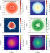 |
Fig. 13 Same as Figure 12, but for run 25. |
| In the text | |
|
Fig. 14 Radial surface density profiles for run 13 of the total gas density (blue solid), stellar density (orange dashed), H2 density (purple dotted), and H I density (green dashed). The curves are normalized to the total gas density in the innermost bin (i.e., at the center). |
| In the text | |
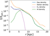 |
Fig. 15 Same as Figure 14, but for run 25. |
| In the text | |
|
Fig. 16 CO(1–0) luminosity images, viewed face-on, for the six different runs analyzed in this paper, after ∆t = 0.2 Gyr from the end of the relaxation phase. The run each image refers to is reported inside the corresponding panel. |
| In the text | |
|
Fig. 17 CO SLED for the baseline analysis of the six simulations studied in this work, after ∆t = 0.2 Gyr from the end of the relaxation phase. The thin red lines display the literature results for different galaxies at cosmic noon. |
| In the text | |
|
Fig. 18 Gas mass surface density maps, viewed face-on, for run 13, after ∆t = 0.1 Gyr (top left), ∆t = 0.2 Gyr (top right), ∆t = 0.5 Gyr (bottom left), and ∆t = 0.8 Gyr (bottom right) from the end of the relaxation phase, respectively. |
| In the text | |
|
Fig. 19 Gas mass surface density maps, viewed face-on, for run 25, after ∆t = 0.1 Gyr (top left), ∆t = 0.2 Gyr (top right), ∆t = 0.5 Gyr (bottom left), and ∆t = 0.8 Gyr (bottom right) from the end of the relaxation phase, respectively. |
| In the text | |
|
Fig. 20 Top: Comparison of the SED predictions for run 13 at different time snapshots, ∆t = 0.1 Gyr (blue solid), ∆t = 0.2 Gyr (orange dashed), ∆t = 0.5 Gyr (purple dotted), and ∆t = 0.8 Gyr (green dotted- dashed) after the end of the relaxation phase, respectively. Bottom: Ratios between the SED of each studied case and the baseline (∆t = 0.2 Gyr). |
| In the text | |
|
Fig. 21 Top: Comparison of the SED predictions for run 25 at different time snapshots, ∆t = 0.1 Gyr (blue solid), ∆t = 0.2 Gyr (orange dashed), ∆t = 0.5 Gyr (purple dotted), and ∆t = 0.8 Gyr (green dotted- dashed) after the end of the relaxation phase, respectively. Bottom: Ratios between the SED of each studied case and the baseline (∆t = 0.2 Gyr). |
| In the text | |
|
Fig. 22 Total CO(1–0) luminosity at different time snapshots normalized to the total CO(1-0) luminosity ∆t = 0.2 Gyr after the relaxation phase, for run 13 (blue solid) and run 25 (orange dashed). The red dotted-dashed line marks unity ratios. |
| In the text | |
|
Fig. A.1 CO(1–0) line spectra for run 13, obtained projecting the galaxy edge-on. The top panel shows the comparison between the spectrum obtained in LTE approximation (blue solid) and the one obtained adopting the non-LTE method (orange dashed). The bottom panel displays the wavelength-wise ratio between the spectra, highlighting that the difference is ≲1% in almost all bins. |
| In the text | |
|
Fig. A.2 Results from the baseline analysis for run 16 (orange dashed) and run 22 (blue solid). Top: SED predictions as a function of the simulation’s resolution (number of SPH particles). Bottom: ratios between the SED of each studied case and the baseline, with the light and dark gray bands showing a 10% and 20% difference, respectively. |
| In the text | |
|
Fig. A.3 Same as Figure 11, but for runs 22 and 16, i.e., as a function of the simulations resolution (number of SPH particles). |
| In the text | |
|
Fig. A.4 Maximum percentage uncertainty on the SED as a function of the number of photons used in the Monte Carlo dust radiative transfer simulations. Sub-percent convergence is reached for nphot = 107 . |
| In the text | |
Current usage metrics show cumulative count of Article Views (full-text article views including HTML views, PDF and ePub downloads, according to the available data) and Abstracts Views on Vision4Press platform.
Data correspond to usage on the plateform after 2015. The current usage metrics is available 48-96 hours after online publication and is updated daily on week days.
Initial download of the metrics may take a while.