| Issue |
A&A
Volume 696, April 2025
|
|
|---|---|---|
| Article Number | A122 | |
| Number of page(s) | 19 | |
| Section | Stellar atmospheres | |
| DOI | https://doi.org/10.1051/0004-6361/202453295 | |
| Published online | 14 April 2025 | |
Discovery of a pair of very metal-poor stars enriched in neutron-capture elements
The proto-disk r-II star BPS CS 29529-0089 and the Gaia-Sausage-Enceladus r-I star TYC 9219-2422-1★
Nicolaus Copernicus Astronomical Center, Polish Academy of Sciences,
ul. Bartycka 18,
00-716
Warsaw, Poland
★★ Corresponding author; This email address is being protected from spambots. You need JavaScript enabled to view it.
Received:
4
December
2024
Accepted:
26
February
2025
Abstract
Context. R-process enhanced metal-poor stars ([Eu/Fe] ≥ +0.3 and [Fe/H] ≤ −1.0) are rare objects, the study of which can provide clues as to the astrophysical sites of the rapid neutron capture process.
Aims. In this study, we investigate the detailed chemical abundance patterns of two of these anomalous stars, originally identified among stars observed by the GALAH survey. Our aim is to obtain the detailed chemical abundance pattern of these stars with spectroscopy at a higher resolution and signal-to-noise ratio.
Methods. We used a calibration of the infrared flux method to determine accurate effective temperatures, and Gaia parallaxes together with broadband photometry and theoretical bolometric corrections to determine surface gravity. Metallicities and chemical abundances were determined with model atmospheres and spectrum synthesis. We also integrated stellar orbits for a complete chemodynamic analysis.
Results. We determined abundances for up to 47 chemical species (44 elements), of which 27 are neutron-capture elements. Corrections because of deviations from the local thermodynamical equilibrium were applied to the metallicities and 12 elements. We find that one of the stars, BPS CS 29529-0089, is a proto-disk star of the Milky Way of r-II type, with [Eu/Fe] = +1.79 dex. The second star, TYC 9219-2422-1, is part of the halo and associated with the Gaia-Sausage-Enceladus merger event. It is of r-I type with [Eu/Fe] = +0.54. Abundances of Th are also provided for both stars.
Conclusions. BPS CS 29529-0089 is the most extreme example of an r-process enhanced star known with disk-like kinematics and not carbon enhanced. TYC 9219-2422-1 is found to be an archetypal Gaia-Sausage-Enceladus star. Their abundances of C, Mg, Ni, Sc, Mn, and Al seem consistent with expectations for stars enriched by a single population III core collapse supernova, despite their relatively high metallicities ([Fe/H] ∼ −2.4).
Key words: stars: abundances / stars: chemically peculiar / stars: Population II / Galaxy: disk / Galaxy: halo / Galaxy: stellar content
Based on observations made with ESO Telescopes at the La Silla Paranal Observatory under programme ID 0108.D-0626(A) and 65.L-0507.
© The Authors 2025
 Open Access article, published by EDP Sciences, under the terms of the Creative Commons Attribution License (https://creativecommons.org/licenses/by/4.0), which permits unrestricted use, distribution, and reproduction in any medium, provided the original work is properly cited.
This article is published in open access under the Subscribe to Open model. This email address is being protected from spambots. You need JavaScript enabled to view it. to support open access publication.
1 Introduction
Old, metal-poor stars offer valuable information for understanding the formation and evolution of our Galaxy (Beers & Christlieb 2005). As long-lived low-mass stars, they are thought to have preserved the chemical properties of the local interstellar medium at the place and time of their formation. One can speculate that the material that formed some of these stars was enriched by only one or maybe a few nucleosynthetic sources (Frebel & Norris 2015). Therefore, the study of their chemical composition may give an unique insight into the first few generations of stars that marked the early history of Galactic chemical enrichment.
Interestingly, some of these old stars have been found to be enriched in r-process elements (Sneden et al. 2008). The rapid neutron capture process (r process, see e.g. Cowan et al. 2021) is a nucleosynthetic mechanism that produces the heaviest elements in the periodic table, along with the slow neutron capture process (s process, e.g. Lugaro et al. 2023) and possibly the intermediate neutron capture process (i process, see e.g. Choplin et al. 2023). The three mechanisms differ with respect to the neutron flux that affects the material and the comparative timescales between successive neutron captures and the beta decay (Arcones & Thielemann 2023). Importantly in this context, the astrophysical sources of the r-process elements are still a mystery.
After neutron capture was proposed as the origin of the heavy elements (Burbidge et al. 1957), several astrophysical sources were suggested as the site where such mechanisms could take place. Among the sites proposed to explain the r process is the merger of degenerate matter objects, such as double systems containing a black hole and a neutron star (BH-NS, Lattimer & Schramm 1974) or two neutron stars (NS-NS, Symbalisty & Schramm 1982). Li & Paczyński (1998) later proposed that such mergers would be accompanied by a transient event, now usually called a kilonova or a macronova.
In this regard, AT 2017gfo (the optical counterpart of the gravitational wave event GW170817, Abbott et al. 2017; Coulter et al. 2017; Valenti et al. 2017) was the first such event to clearly associate a neutron star merger (NSM) with neutron-capture element production (Tanvir et al. 2017; Pian et al. 2017). The list of elements with features identified in the AT 2017gfo spectra includes Sr (Watson et al. 2019), La III and Ce III (Domoto et al. 2022), and Te (Hotokezaka et al. 2023). On the other hand, elements such as Au and Pt were searched for but not found (Gillanders et al. 2021). Currently, there is an active debate about whether lanthanide-poor or lanthanide-rich models better reproduce the spectral evolution of AT 2017gfo (Domoto et al. 2021; Vieira et al. 2024).
Other possible sites of r-process nucleosynthesis include different types of supernovae and hypernovae (see Cowan et al. 2021, and references therein). However, there has still been no clear observational confirmation of the production of r-process elements at any other astrophysical site. In fact, the topic remains highly debated, and sometimes disparate conclusions are reached. For example, Siegel (2019) argue that collapsars (high-mass stars that produce a black hole in their collapse, together with a long-duration gamma-ray burst and a hypernova) could supply about 80% of the r-process elements in the Universe. However, the work of Bartos & Marka (2019) indicates that collapsars could possibly contribute less than 20% of the r-process elements found in the Solar System. In connection with that, it is worth mentioning that the supernova associated with the long-duration gamma-ray burst GRB 221009A, the brightest observed to date, was found to lack an r-process signature (Blanchard et al. 2024).
The current era of large astrometric, photometric, and spectroscopic stellar surveys, such as Gaia (Gaia Collaboration 2016), S-PLUS (Southern Photometric Local Universe Survey, Mendes de Oliveira et al. 2019; Perottoni et al. 2024), J-PLUS (Javalambre-Photometric Local Universe Survey, Cenarro et al. 2019), APOGEE (Apache Point Observatory Galactic Evolution Experiment, Majewski et al. 2016), Gaia-ESO (Randich et al. 2022) and GALAH (GALactic Archaeology with HERMES, De Silva et al. 2015), give us the opportunity to identify and study larger samples of metal-poor stars (e.g. Da Costa et al. 2023; Placco et al. 2023; Viswanathan et al. 2024; Bonifacio et al. 2024; Hou et al. 2024; Xylakis-Dornbusch et al. 2024). Among these metal-poor stars, it is possible to discover and study objects with unusual r- and s-process abundance patterns, including those that are enriched and/or depleted in such elements (e.g. François et al. 2007; Holmbeck et al. 2020; Placco et al. 2023; Saraf et al. 2023; Sestito et al. 2024). All of these data provide a unique opportunity to obtain a holistic view of all possible sources of the r process.
R-process enriched stars (RPEs) have traditionally been classified as r-I and r-II (Beers & Christlieb 2005), whereby r-I stars are ones with moderate enrichment of the r process with 0.3 ≤ [Eu/Fe] ≤ +1.0 dex and the r-II stars are ones with extreme r-process enrichment with [Eu/Fe] ≥ +1.0 dex. Early studies such as Sneden et al. (1994) and Hill et al. (2002) were already able to find a few examples of RPEs with quiet high [Eu/Fe] ratios, ≥ +1.6 dex. Nevertheless, such objects are rare. Ezzeddine et al. (2020) report on a sample of253 RPEs, ofwhich only 7.4% are r-II. Moreover, recently a new class of super RPEs, the r-III, was proposed to account for a few of the most extreme objects with [Eu/Fe] ≥ +2.0 dex (Cain et al. 2020; Roederer et al. 2024).
The Stellar Abundances for Galactic Archeology (SAGA) database1 (Suda et al. 2008) lists 26 stars with [Eu/Fe] ≥ +1.7 dex. Of these, 21 are also carbon-enhanced metal-poor (CEMP, [C/Fe]≥ +1.0) stars belonging to the Milky Way. Moreover, Roederer et al. (2024) discuss four additional stars that are not in the SAGA database, with [Eu/Fe] ≥ +1.7 dex: TYC 8100-833-1, SMSS J145341.38+004046.7 (Ezzeddine et al. 2020), TYC 7325920-1 (Cain et al. 2020), and TYC 8444-76-1 (Roederer et al. 2024). To our knowledge, the star with the highest nominal [Eu/Fe] reported to date is BPS CS 31070-0073, a CEMP-r star with [Eu/Fe] = +2.83(25)2 (Allen et al. 2012).
The vast majority of known RPEs are kinematically part of the Milky Way’s halo population, with only about 10% potentially being members of the disk (Gudin et al. 2021). Those belonging to the halo include stars that formed in situ in the Milky Way as well as accreted stars (Roederer et al. 2018a,b). A major source of RPEs seems to be the Gaia-Enceladus merger event, a possible origin of about 20% of the halo RPEs (Yuan et al. 2020; Gudin et al. 2021; Limberg et al. 2021). The Gaia-Enceladus event, discovered from Gaia DR2 data (Belokurov et al. 2018; Helmi et al. 2018), is believed to have been the last major merger to have taken place in the Milky Way (but see Donlon et al. 2024, for a different view). Gaia-Enceladus completed its merger about 9.6 billion years ago (Giribaldi & Smiljanic 2023b). On the other hand, Xie et al. (2024) recently reported the first RPE with thin disk kinematics which has [Eu/Fe] = +1.32(13) but is not very metal-poor, with [Fe/H] = −0.52. Johnson et al. (2013) found an RPE star in the bulge of the Galaxy. Two other examples of RPE have also been reported in the inner Galaxy and the Bulge, thanks to increased efforts to identify metal-poor stars in these regions (Forsberg et al. 2023; Mashonkina et al. 2023). In addition to the Milky Way, other stars with [Eu/Fe] ≥ +1.7 dex have been found in the dwarf galaxy Reticulum II (Ji et al. 2016), in the Fornax dwarf galaxy (Reichert et al. 2021), in the Large Magellanic Cloud (Reggiani et al. 2021), and in the Indus stellar stream (Hansen et al. 2021).
In this work, we report a detailed chemical abundance analysis of two new examples of r-process-enhanced very metal-poor stars ([Fe/H] < −2). A total of 47 chemical species, including 27 neutron-capture elements, were investigated. These two stars are part of an observational program that we started with the aim of providing detailed chemical abundances for a new set of RPEs. As is discussed in the next sections, our results indicate that one star (BPS CS 29529-0089) was probably formed in the proto-disk of the Milky Way, while the other (TYC 92192422-1) was probably part of the Gaia-Enceladus system. BPS CS 29529-0089 is the metal-poor star with disk kinematics with the highest known [Eu/Fe] that is not a CEMP. This work is organized as follows. We present the selection criteria, observational setups, and analysis methods in Section 2. The results are presented in Section 3 and their implications are discussed in Section 4. Finally, our conclusions are summarized in Section 5.
2 Methods
2.1 Sample selection and observations
The two stars that we discuss here, BPS CS 29529-0089 and TYC 9219-2422-1, were selected from the GALAH survey. As of data release 3 (Buder et al. 2021), the one used in this work, GALAH provides up to 30 elemental abundances for 588 571 stars, including elemental abundances for two neutron capture elements, Ba and Eu. As the sample of our observational program, we selected very metal-poor ([Fe/H] ≤ −2) GALAH stars that had values of [Eu/Fe] and [Ba/Fe] that differed by more than 3 σ from the mean of the whole sample (see Fig. 1). For this selection, we did not take into consideration the quality flags of GALAH abundances, as using these flags could exclude outlier stars with uncertain but high Eu and Ba abundances, which are exactly the kind of stars that we are interested in. In total we selected 167 candidates that had Johnson V band magnitudes in the literature. As a pilot study, to test whether we were indeed selecting real examples of RPE, we decided to first observe the two most anomalous and bright stars: TYC 9219-2422-1 and BPS CS 29529-0089.
The two stars were observed with the Ultraviolet and Visual Echelle Spectrograph (UVES, Dekker et al. 2000) at the Very Large Telescope of the European Southern Observatory (ESO). Two spectra were obtained for TYC 9219-2422-1 and three spectra for BPS CS 29529-0089, with a resolving power (R) of ~41600 and signal-to-noise ratio (S/N) of ~50 at 372.4 nm. The wavelength range was divided into two arms, a blue one centered at 390 nm and a red one centered at 580 nm (see details in Table 1). For comparison purposes, we also analyzed spectra of the Gaia benchmark star HD 122563 (Jofré et al. 2014). The HD 122563 spectra that we analyzed were taken from the UVES Paranal Observatory Project archive (Bagnulo et al. 2003) and observed with spectrograph setups identical to the two stars in our program. Data reduction was performed using the UVES pipeline (Ballester et al. 2000). Using iSpec (Blanco-Cuaresma et al. 2014; Blanco-Cuaresma 2019), we determined radial velocities (P) and barycentric corrections, placed them in the rest frame, and combined the multiple spectra of each star.
Observations.
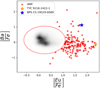 |
Fig. 1 Selection of anomalous stars in GALAH DR3. In gray scale is a 2D histogram of all stars in GALAH DR3 with Ba and Eu abundances. The red ellipsis marks the region differing by 3 σ from the mean abundances. The red star symbols show the anomalous stars that also have [Fe/H] ≤ 2. The two stars analyzed here are shown in different colors. |
2.2 Atmospheric parameters
The effective temperatures (Teff) were derived iteratively with the infrared flux method (IRFM) calibrations of Casagrande et al. (2021) by means of the code colte3, using the photometric bands of the Two Micron All Sky Survey (2MASS, Skrutskie et al. 2006) and Gaia (Riello et al. 2021). Values of Teff determined with such calibrations tend to have a very good accuracy (Giribaldi et al. 2021, 2023). The photometric data for BPS CS 29529-0089 and TYC 9219-2422-1 are given in Table 2.
The values of surface gravity (log g) were determined with Gaia parallaxes (Gaia Collaboration 2021), corrected by the biases using the tool made available by Lindegren et al. (2021), and bolometric correction computed with the method from Masana et al. (2006). The extinction values were obtained using the Galactic Dust Reddening and Extinction service from the InfraRed Science Archive (IRSA)4 and corrected using the recipe from Beers et al. (2002).
Metallicities ([Fe/H]) were determined using Fe II lines that have good values of oscillator strengths( log gf) given in Meléndez & Barbuy (2009) (see Table 3 for the list of lines we used). We chose to use Fe II lines as they tend to be less sensitive to departures from the local thermodynamical equilibrium (the so-called non-LTE effects) compared to neutral Fe lines. The Fe II lines were fit with synthetic spectra calculated with TSFitPy5, a Python wrapper for the Turbospectrum NLTE6 code (Gerber et al. 2023; Plez 2012). For the calculations, we assumed a fixed microturbulence velocity (vmic) of 1.5 km s−1, used MARCS model atmospheres (Gustafsson et al. 2008), and adopted the solar abundances from Asplund et al. (2009) modified by Magg et al. (2022). The atmospheric parameters determined for our two sample stars are given in Table 4. For HD 122563, we adopted the accurate values of Teff and log g determined by Giribaldi et al. (2023) with a revised metallicity value7.
Uncertainties in Teff are provided by colte and come from Monte Carlo simulations using the uncertainties of the photometric bands. For the log g uncertainties, we applied a Monte Carlo to the photometric bands, Teff, parallax, and [Fe/H] over their uncertainties (the standard deviation in the case of metallicity) and added the systematic uncertainty in the bolometric correction presented in Masana et al. (2006). We adopted a fixed uncertainty for vmic of 0.1 km s−1. The fixed values adopted here for vmic and its uncertainty are consistent with what was found, for example, by Limberg et al. (2024) for metal-poor stars of similar surface gravity. For [Fe/H], we reran TSFitPy to determine the effect of changing the other atmospheric parameters (Teff, log g, and vmic) by their uncertainties.
Photometric data.
List of Fe II lines used in this work.
2.3 Chemical abundances
Chemical abundances were determined by spectral synthesis. The order for the determination of abundances followed the periodic table (ascending Z), except for the carbon abundance, which was the first to be determined. To account for possible blends because of the enhanced lines of heavy elements, the abundance determination loop was run twice. In the second time, all abundance values found in the first run were used as input values. We generated grids of spectra using TSFitPy for each spectral line. The grids were generated with values from [X/Fe] = −3.0 dex to [X/Fe] = +3.0 dex in steps of 0.01 and χ2 values were calculated to compare the synthesized spectra and the observed spectrum. Then, a Nelder-Mead optimization algorithm, implemented using scipy (Virtanen et al. 2020), was used to find the minimum. This approach was performed in a region of 1 nm around each spectral line. The final mean abundances are given in Table A.1 and the line-by-line values are available in the data availability Section 5. For elements with multiple spectral lines, the abundance results are the mean with outliers excluded using a 3-σ clipping criterion. Statistical uncertainties are the standard deviation of the line-by-line values. Some selected lines with their respective synthetic fits are shown in Appendix D.
The grid procedure was also applied to estimate the uncertainties of the abundances caused by the errors in the atmospheric parameters. This was done by changing the atmospheric parameters (Teff, log g, [Fe/H], and vmic) up and down by their respective uncertainties and synthesizing spectra spanning 1 dex around the measured value of the abundance in steps of 0.02 dex. These uncertainties are also listed in Table A.1.
Most of the atomic data we used are those compiled by the Gaia-ESO Survey (Heiter et al. 2021), complemented with data taken from the Vienna Atomic Line Database (Vienna Atomic Line Database, Ryabchikova et al. 2015) below 420 nm. In the latter case, the lines are part of the line list compiled and tested as described in Giribaldi & Smiljanic (2023a). When available, we adopted the hyperfine structure (HFS) of the spectral lines in the blue (≤420 nm) from the linemake8 list generator (Placco et al. 2021). For lines in the redder part of the spectra (≥420 nm), the Gaia-ESO (Heiter et al. 2021) HFS data was used. Exceptions to the above are the HFS for the lines of Eu II and Ba II that we recalculated here. In summary, the elements Sc, V, Mn, Co, Nb, Ag, Ba, La, Pr, Nd, Sm, Eu, Tb, Ho, Yb, Lu, Ir, and Pb had HFS taken into account during the spectral synthesis.
For the Eu lines in the blue region (at 3724.9, 3819.7, 3907.1, 3930.5,4129.7, and 4205.0 Å) and the line at 6645.1 Å in the red, we recalculated the HFS taking into account isotopic splitting (isotopes with A = 151 and 153), adopting the data from Lawler et al. (2001). For the Ba lines at 5853.67, 6141.71, and 6496.90 Å, the calculations used the isotopic splitting and HFS data from Van Hove et al. (1982) and Villemoes et al. (1993). Hyperfine splitting is only important for isotopes with A = 135 and 137, but lines for isotopes with A = 134, 136, and 138 are also taken into account, as they are present in important amounts. The energy shifts and line strengths were calculated as in Smiljanic et al. (2023) with the help of the code made public by Mathar (2011) and equations that can be found, for example, in Emery (2006). The data for the Eu lines can be found in Appendix B and for the Ba lines in Appendix C.
When possible, abundances were corrected for non-LTE effects, adopting atomic models and lists already available in TSFitPy (Gerber et al. 2023). The list of elements and references for the corrections is as follows: Al and Na (Ezzeddine et al. 2018) and (Nordlander & Lind 2017), Y (Storm & Bergemann 2023), Sr (Bergemann et al. 2012), Ba (Gallagher et al. 2020), Ni (Bergemann et al. 2021), Ti (Bergemann 2011), Co (Bergemann et al. 2010), Fe (Bergemann et al. 2012), Mn (Bergemann et al. 2019), Mg (Bergemann et al. 2017), and Ca (Mashonkina et al. 2017).
Atmospheric parameters of the stars.
Positions and kinematics of the target stars.
2.4 Dynamics
We integrated the stellar orbits using Gaia DR3 data (coordinates, parallaxes and proper motions, Gaia Collaboration 2021). We used the Python code galpy (Bovy 2015) to integrate the orbits assuming the McMillan (2017) Milky Way potential. The integration lasted for 13 Ga9 backward in steps of 260 Ma. A Monte Carlo simulation was performed on the uncertainties of the positions, velocities, and parallaxes. We analyzed these stars in a similar manner to da Silva & Smiljanic (2023).
3 Results
As was mentioned in Section 2, we selected a sample of GALAH stars ignoring the quality flags of the Ba and Eu abundances. However, it turns out that the [Ba/Fe] in both TYC 9219-24221 and BPS CS 29529-0089, selected for this pilot study, have flag 0 (indicating reliable values) in GALAH DR3. The abundances of Ba for the two stars in GALAH agree well with the values determined here. The [Eu/Fe] for BPS CS 29529-0089 is also very close to ours. These similarities are somewhat surprising, as the GALAH effective temperatures differ from our values by about 2σ. In GALAH DR3, Teff values were derived spectroscopically through the Fe excitation and ionization equilibria. GALAH also provide alternative Teff values based on the IRFM from Casagrande et al. (2021) and those values differ from ours by only 11 K. As for [Eu/Fe] in TYC 9219-2422-1, GALAH only provides an upper limit (indicated by flag 1 in the GALAH tables) of +2.34(14), which is much higher than the value derived here.
3.1 Light elements and Fe-peak
We present the chemical abundances in Table A.1. The three stars analyzed in this study have low carbon abundances ([C/Fe]< 1.0) and are therefore not part of any CEMP subclass of metalpoor star. Carbon corrections based on the evolutionary status of the stars (Placco et al. 2014)10 for BPS CS 29529-0089 and TYC 9219-2422-1 are on the same order of magnitude as the abundance uncertainties. However, for HD 122563 the carbon correction is 0.74, bringing its actual [C/Fe] ratio to about 0.06 dex.
We tried to derive the abundances of N using the CN molecular bands between 387.5 and 390.0 nm; however, those CN lines were found to be too faint. The forbidden oxygen line at 630.03 nm in both BPS CS 29529-0089 and TYC 9219-2422-1 is unfortunately contaminated by a telluric line.
The Li abundances were measured using the doublet lines around 670.7 nm. BPS CS 29529-0089 presents A(Li)= 1.23 and TYC 9219-2422-1 A(Li) = 1.29 while HD 122563 A(Li)= −0.28. These values put both BPS CS 29529-0089 and TYC 9219-2422-1 at the Li plateau of metal-poor red giants discovered by Mucciarelli et al. (2022), which is consistent with the Spite plateau (Spite & Spite 1982) of lithium measured in metalpoor dwarfs after the dilution by evolutionary effects is taken into account.
The α elements (Mg, Si, and Ca) are enhanced in all three stars, as was expected, in particular after non-LTE corrections are taken into account (see Ca for HD 122563). Aluminum in the three stars is well below the solar [Al/Fe] ratio, with TYC 92192422-1 and BPS CS 29529-0089 presenting [Al/Fe] < −0.7 dex. We also find that the three stars have low manganese abundances ([Mn/Fe] < 0.0 dex). We refrain from discussing the stars in the [Mg/Mn] versus [Al/Fe] plane, as an indicator of accreted origin, as this has mostly been used for stars with [Fe/H] > −2.0 (Das et al. 2020).
Apart from Mn, the other iron peak elements between Sc and Zn in BPS CS 29529-0089 mostly exhibit [Element/Fe] ratios close to solar. The only exception is Cr, which is found to be quite low at [Cr/Fe] = −0.51. Interestingly, TYC 9219-2422-1 tends to have [Element/Fe] ratios that are 0.1 to 0.2 dex higher than BPS CS 29529-0089 in all these elements. An even-odd effect can be observed in the abundances from C to Zn in both BPS CS 29529-0089 and TYC 9219-2422-1.
For HD 122563, the abundance levels are all below solar. Abundances of iron-peak elements for HD 122563 have been determined, for example, by Barbuy et al. (2003). Our [Ele- ment/Fe] ratios are, on average, −0.13 dex lower than the values obtained by Barbuy et al. (2003). However, their metallicity value ([Fe/H] = −2.71) is lower than the one we adopted by 0.12 dex. This difference essentially fully explains the difference in [Element/Fe] ratios.
3.2 Neutron capture elements
Our results show that the Gaia-Benchmark HD 122563 presents no enrichment in neutron capture elements. This is in agreement with previous results in the literature (Honda et al. 2006). The [Y/Fe] we determined in LTE ([Y/Fe] = −0.59) is actually within the interval presented by the NLTE analysis of Storm & Bergemann (2023) (see bottom panel of Fig. 8 of their paper).
TYC 9219-2422-1 presents a moderate but clear enrichment in neutron capture elements. Our new measurement of [Eu/Fe] = 0.54(12) together with [Ba/Eu] = −0.70 (in LTE), indicates that TYC 9219-2422-1 is an r-I star. BPS CS 29529-0089 is found to have a stronger enrichment in neutron-capture elements. Star BPS CS 29529-0089 has [Eu/Fe] = 1.79 and [Ba/Eu] = −0.76 (LTE). BPS CS 29529-0089 is thus a r-II star and the abundances point to a probable r-process-only enrichment (see Bisterzo et al. 2014). We compare the [Eu/Fe] levels of BPS CS 29529-0089 and TYC 9219-2422-1 with 379 non-CEMP stars from the JINA database11 (Abohalima & Frebel 2018) in the same manner as Cain et al. (2020) (see Fig. 2).
We detected Th in both BPS CS 29529-0089 and TYC 92192422-1, but the lines of uranium could not be detected. The high abundance of Th indicates an actinide-rich environment forming BPS CS 29529-0089. A fraction of metal-poor stars, mostly below [Fe/H] = −3.0, have been found to be enhanced in Th and U with respect to lighter r-process elements and have been called actinide-boost stars (e.g. Holmbeck et al. 2018; Placco et al. 2023). For BPS CS 29529-0089, we found log є Th/Eu = −0.40, which, although above solar, implies that this star is not part of the actinide-boost class, even though we do not know its uranium abundance.
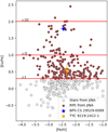 |
Fig. 2 The [Eu/Fe] ratio as a function of [Fe/H]. The stars shown as circles are non-CEMP metal-poor stars from the JINA database (Abohalima & Frebel 2018). Open circles are ordinary stars, while brown ones are RPEs. R-I, r-II, and r-III levels are shown by the red lines. BPS CS 29529-0089 and TYC 9219-2422-1 are shown as colored star symbols. |
4 Discussion
4.1 Chemodynamic analysis
We used the dimensionality reduction algorithm t-SNE (t-distributed stochastic neighbour embedding) for the chemodynamic classification of the stars, in a similar manner as was done in da Silva & Smiljanic (2023). For this analysis, we adopted four quantities, [Fe/H], [Mg/Fe],  and
and  12, as dimensions, and used t-SNE to obtain a projection of the stellar distribution in two dimensions (2D). The 2D projection is shown in Fig. 3. To perform the classification, we also included the stars of the GALAH sample used in da Silva & Smiljanic (2023). The same four groups defined in that work are highlighted in Fig. 3: a group with average zero angular momentum associated with Gaia Enceladus, a second group that is slightly more prograde, a third group that is slightly more retrograde, and a fourth group that includes the most retrograde stars of the sample (see Fig. 4). We recall that da Silva & Smiljanic (2023) found that the Gaia Enceladus group was chemically similar to both the retrograde and prograde groups. Only the most retrograde group showed a distinct chemical composition and was suggested to be dominated by stars from the Sequoia and/or Thamnos mergers (see Myeong et al. 2019; Koppelman et al. 2019). For comparison purposes, we also added to the sample several RPEs from the SAGA database and from Roederer et al. (2024) that have [Eu/Fe] ≥ +1.70 dex.
In the tSNE projection, BPS CS 29529-0089 falls in the region dominated by disk stars (bottom part, with values below ~−20 in the projetion 2 axis). Both HD 122563 and TYC 92192422-1 fall in the other region, dominated by halo objects. The action map shown in Fig. 5 supports this, as BPS CS 295290089 is seen to have an orbit that is prograde, circular, and in the plane. Compared to the action map of Shank et al. (2023), BPS CS 29529-0089 fits their definition of the metal-weak thick disk (MWTD) group. These stars are thought to be primordial proto-disk stars that have migrated due to interactions within the Milky Way or with merger events (Shank et al. 2023). Interestingly, Shank et al. (2023) indicates that the MWTD does not seem to have suffered r-process enrichment events that would create a significant fraction of RPE stars (Shank et al. 2022a,b). This already highlights the uniqueness of BPS CS 29529-0089.
Three other RPE stars fall in the same region as BPS CS 29529-0089 in the t-SNE map: HE 1105+0027, TYC 7325-920-1 and CD-28 1082. However, only two of them (HE 1105+0027 and CD-28 1082) remain close to BPS CS 29529-0089 in the action map (Fig. 5) and in the Lindblad diagram (Fig. 4). TYC 7325920-1, with [Fe/H] = −2.80, [C/Fe] = 0.56, [Ba/Fe] = 1.35, and [Eu/Fe] = 2.23 (Cain et al. 2020), has a high zmax and kinematic and does not match the thick disk (see Table A.2).
However, CD-28 1082 and HE 1105+0027 have thick disk characteristics. CD-28 1082 ([Fe/H] = −2.45) is highly enhanced in C, Ba, and Eu; [C/Fe] = 2.19, [Ba/Fe] =2.09, and [Eu/Fe] = 2.07 (Purandardas et al. 2019; Goswami et al. 2021). HE 1105+0027 ([Fe/H] = −2.42) is similarly enhanced in C, Ba, and Eu; [C/Fe] = 2.00, [Ba/Fe] =2.45, and [Eu/Fe] = 1.81 (Goswami et al. 2021). These stars have dynamic properties similar to BPS CS 29529-0089. This can be easily seen in the Lindblad diagram (Fig. 4) and the action map (Fig. 5), which show only these two stars nearby BPS CS 29529-0089. The characteristic that distinguishes BPS CS 29529-0089 is that it has a normal carbon abundance. This star seems to be the only known very metal-poor r-II star belonging to the old disk.
Our second target, TYC 9219-2422-1 falls on the prograde group that da Silva & Smiljanic (2023) associated to Gaia - Sausage-Enceladus (see e.g. Helmi et al. 2018; Belokurov et al. 2018). Aguado et al. (2021) and Matsuno et al. (2021) report a [Ba/Fe] ≤ 0.0 and [Eu/Fe] ~ +0.5 which is in good agreement with TYC 9219-2422-1. da Silva & Smiljanic (2023) showed that the Gaia-Sausage-Enceladus stars have [Eu/Mg] ~ 0.40 in the metallicity interval between about −0.8 and −1.7. More recently, Monty et al. (2024), Ou et al. (2024) and Ernandes et al. (2024) found that the [Eu/α] ratio decreases for metallicities below that interval, reaching [Eu/α] ~ 0.0 (with some scatter) at the metallicity of TYC 9219-2422-1. As discussed in Ou et al. (2024), for example, delayed r-process sources, such as NSMs, are needed to explain the increase in the [Eu/Mg] ratio with increasing metallicity. We compare TYC 9219-2422-1 with stars in Ou et al. (2024) in Fig. 7. Its position on the [Mg/H] by [Eu/Mg] plane matches the position of the other stars in the magnesium-poor tail of their sample.
In our analysis, HD 122563 falls on Gaia-Sausage- Enceladus group proper (the one with average zero angular momentum in Fig. 4). However, it terms of its chemistry, besides [Fe/H] and [Mg/Fe] values that agree with Gaia-Sausage- Enceladus, HD 122563 is extremely poor in neutron capture elements. Therefore, we suggest that HD 122563 is instead part of the in situ population that contaminates this region of the parameter space (as discussed in da Silva & Smiljanic 2023, in situ populations seem to be present in all groups that were investigated in that work).
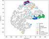 |
Fig. 3 Projection map obtained using t-SNE. The gray stars are the sample from GALAH used in da Silva & Smiljanic (2023). The four groups defined in that work (Gaia Enceladus, prograde, retrograde, and most retrograde) are colored in green, blue, light brown, and dark purple, respectively. The cyan stars are 28 RPE stars with [Eu/Fe] ≥ + 1.7 dex found in the SAGA database (Soubiran et al. 2024) complemented by five stars from Roederer et al. (2024). The Sun is added as reference. |
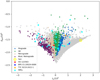 |
Fig.4 Lindblad diagram (Lz × En). Coloring is the same as Fig. 3. Error bars are smaller than the size of the symbols. |
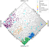 |
Fig. 5 Action map. Coloring is the same as Fig. 3. Note BPS CS 29529- 0089in the most prograde, circular and in the plane orbits. Error bars are smaller than the size of the symbols. |
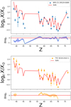 |
Fig. 6 Top: comparison of the solar r-process abundance pattern with the abundances of BPS CS 29529-0089. Bottom: same comparison for TYC 9219-2422-1. |
4.2 BPS CS 29529-0089 as part of the proto-disk population
As was mentioned in the introduction, RPEs have been shown to generally be part of the halo stellar population. As such, they are either accreted stars from dwarf galaxies that merged with the Milky Way, from systems maybe similar to ultra-faint dwarf galaxies or dwarf spheroidals (see e.g. Ji et al. 2016; Reichert et al. 2020, 2021), or they are part of the in situ halo of our Galaxy. In support of the idea of accreted origin, RPEs have been found in streams such as Indus (Hansen et al. 2021) and in dwarf galaxies such as Fornax (Ji et al. 2016) and Reticulum II (Reichert et al. 2020). Some studies have shown that a fraction (~ 10%) of RPE stars with an origin in the Milky Way display disk dynamics (see e.g Gudin et al. 2021; Shank et al. 2022a). More recently, the first thin-disk RPE star (with [Fe/H] > −1.0) was discovered (Xie et al. 2024).
Cosmological zoom-in simulations of Milky Way-like galaxies could shed light on where RPE form. In this context, Hirai et al. (2022, 2024) simulated the formation of small stellar systems that were later accreted into a Milky Way-like galaxy. Both studies concluded that RPE stars more easily form in small dwarf systems. This is due to the fact that a single NSM can significantly increase the abundance of r-process elements in these systems because of their relatively low gas mass. Observationally, Limberg et al. (2024) note that on these small systems a delayed source is enough to explain the r-process enrichment.
Hirai et al. (2022, 2024) also found that in situ RPEs can be formed. This occurs in clumps contaminated with NSM ejecta in which mixing has not had enough time to dilute the enrichment before new stars are formed. Hirai et al. (2022) point out that around 90% of r-II stars with [Fe/H] ≤ −2 in a Milky-Way like galaxy have accreted origins. In the newer study, they point out that less than 20% of stars with +1.5 ≤[Eu/Fe] ≤ +1.9 would have an in situ origin. Moreover, Hirai et al. (2024) found that only 0.2% of r-II RPE stars have an origin in the in situ component of their simulation. Together, the results discussed above show that there is a plausible scenario in which an r-II star forms on the Milky Way disk and confirm that BPS CS 29529-0089 is an example of a very rare object.
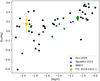 |
Fig. 7 [Mg/H] by [Eu/Mg] plane. Black circles are stars from Ou et al. (2024), green squares are stars from MINCE (Cescutti et al. 2022; François et al. 2024, as cited in Ou et al. 2024), and blue triangles are stars from Aguado et al. (2021). TYC 9219-2422-1 is the orange star. |
4.3 Stellar abundances and the origin of their r-process elements
Complete inventories of chemical abundances in metal-poor stars are somewhat rare in the literature. Some examples of RPE with more than 35 elemental abundances derived are: HD 222925 (Roederer et al. 2022), 2MASS J22132050-513785 (Roederer et al. 2024), 2MASS J00512646-1053170 (Shah et al. 2024), HD 20 (Hanke et al. 2020), and BPS CS 31082-001 (Hill et al. 2002; Ernandes et al. 2022, 2023). For our target BPS CS 29529-0089, we provide abundances for 44 elements, of which 27 are neutron-capture elements. This is a slightly higher number of elements than was found for HD 222925 (Roederer et al. 2022) using only ground UV and the visible part of the spectrum. Thus, BPS CS 29529-0089 is an excellent candidate for space UV observations, ≤3000 Å, to increase the number of neutroncapture elements with abundances, possibly including some rare elements like gold.
In Fig. 6, we compare our results with the solar r-process abundance pattern. To obtain the solar r-process component, we subtracted the expected contribution of the s-process using the fractions from Bisterzo et al. (2014). In the comparison, we normalize the abundance pattern to the Eu abundance. For BPS CS 29529-0089, the most significant deviations occur for elements with Z < 50. Such deviations have been seen before in other stars and have been attributed to the contribution of a weak r process (or similar mechanism) to the solar material. This process is believed to synthesize lighter elements such as Sr (Z = 38), Y (Z = 39), and Zr (Z = 40), but it is not able to produce heavier than the first-peak r-process elements (Siqueira Mello et al. 2014; Xing et al. 2024). In contrast, TYC 9219-2422-1 appears to follow the solar r-process pattern for these lighter elements more closely, but we see some discrepancy in the abundances of Ce (Z = 58) and Nd (Z = 60). Finally, for both stars, ytterbium (Yb, Z = 70) stands out as an element that does not align with the expected pattern.
To gain some insight into the possible origins of abundances in BPS CS 29529-0089 and TYC 9219-2422-1, we used starfit13 (Heger & Woosley 2010). The code starfit compares the measured abundance pattern in a star to a series of model abundances from different possible progenitors. Here we used the option with a genetic algorithm to choose the best-fitting model(s) among the calculations of Heger & Woosley (2010), Mendoza-Temis et al. (2015), and Wu et al. (2016).
Our choice of models for starfit means that we are searching only for solutions that combine one population III (pop III) core collapse supernova (SN) with a second source responsible for the r process. This does not need to be the correct combination of sources needed to explain the abundances in our two stars. In fact, given their relatively high metallicity, [Fe/H] = −2.3 to −2.5, we should anticipate that there is a low probability that the stars are direct descendants of pop III SNe. Nevertheless, there are theoretical simulations that indicate that a single pop III SN could enrich the surrounding medium to a level close to [Fe/H] = −2.0 (e.g. Smith et al. 2015). Moreover, the work of Hartwig et al. (2018) shows that other chemical abundances, in addition to Fe, are important in the search for such monoenriched stars. These authors investigated regions of the chemical abundance parameter space with high probability of being populated by second-generation stars enriched by a single pop III supernova.
Following Hartwig et al. (2018), we looked at the abundances of C, Mg, Ni, Sc, Mn, and Al (in addition to Fe) compared to their chemical divergence maps (see their Fig. 18). For BPS CS 29529-0089, we have [Mg/C] = 0.30(13) dex, [C/Ni] = 0.04(17) dex, and [Sc/Mn] = 0.39(16) dex, while for TYC 9219-2422-1, the corresponding values are [Mg/C] = 0.27(14) dex, [C/Ni] = 0.07(23) dex, and [Sc/Mn] = 0.61(19) dex. These measurements place both BPS CS 29529-0089 and TYC 9219-2422-1 within the regions dominated by mono-enriched stars in Fig. 18 of Hartwig et al. (2018). However, we remark that, as is discussed in Hartwig et al. (2018), this comparison does not give a probability that the stars are mono-enriched. It simply shows that in the chemical abundance space they are located in a region dominated by mono-enriched stars. There may be other means for such abundances to be obtained apart from a single pop III star. In any case, this comparison indicates that it is interesting to use starfit to search for pop III progenitors that could explain our two stars.
A fit for the abundance pattern of TYC 9219-2422-1 is provided in Fig. 8. From this fit, the most probable phenomenon leading to the chemical abundance pattern of this star is a combination between one pop III supernovae, with the progenitor mass of 10.7 M⊙ (fitting the lighter elements with the even-odd pattern until Zn), with a NSM r-process phenomenon occurring 13 Ga ago (fitting heavier elements from Sr upwards). If correct, this fit would agree with the findings of Ernandes et al. (2024), pointing to an important enrichment of r-process elements coming from NSM in stars of Gaia-Sausage-Enceladus.
The abundance pattern for BPS CS 29529-0089 is shown in Fig. 9 in conjunction with the best-fitting models. The abundance pattern of BPS CS 29529-0089 indicates a combined contribution from a pop III SN with 15 M⊙ and a NSM r-process enrichment 13 Ga ago. The NSM model fits the abundances of this star better than what was seen with TYC 9219-2422-1. A possible NSM origin for the r-process enrichment of BPS CS 29529-0089 is consistent with the scenario proposed in Hirai et al. (2022, 2024) for the formation of such stars in situ in the proto-disk of the Milky Way, as was discussed above.
We note that both stars present an excess in the abundance of the elements around Z∼40 and ∼58 with respect to the models. This could be explained with fission products, as is suggested in Roederer et al. (2023). Fission products are daughter nuclides of spontaneous fission that neutron-rich father nuclides undergo, especially for transuranic elements (with Z ≥ 92). This stochastic process produces pairs of daughter nuclides with a two-peak distribution with maxima around A∼95 or A ∼ 140. Roederer et al. (2023) argue that the strong correlation between the abundances of elements such as ruthenium, rhodium, palladium, and silver points to an excess abundance caused by fission fragments of transuranic elements with a large number of neutrons. In fact, the values of log ϵ (Ru/Zr) = −0.19, log ϵ (Rh/Zr) = −1.05, and log ϵ (Pd/Zr) = −0.48 for BPS CS 29529-0089, are similar to the expected values to be found in case of fission, around −0.18, −0.82, and −0.54, respectively, for the level of [Eu/Fe] seen in the star (see Fig. 8 in Roederer et al. 2024).
As a last point, we note that essentially all heavier neutron capture abundances appear to follow the expected pattern, except for the element Yb. We rechecked its abundance, determined using the Yb II line in 3694Å for the three stars (see Fig. D.8 in Appendix D). We confirmed the values, but we do not have a clear explanation for the apparent deficiency.
4.4 Nucleocosmochronology
Most of the nuclides are unstable. They decay in a stochastic manner with the rate of decay as a function of time. The phenomenon of radioactive decay has been used to determine accurate and precise ages in a series of fields from archaeology to environmental radiometry. Although the use of radioactivity to determine the age of stars has been suggested as a result of its convenience, there are limitations. Specifically, it is not feasible to directly measure radionuclide abundances; only total elemental abundances are accessible, and the initial production ratios remain highly uncertain (Cayrel et al. 2001).
Given the detection of both Th and Hf in BPS CS 29529-0089, we decided to try to date this star using nucleocosmochronology. We followed here Kratz et al. (2007), who suggested that the Th/Hf ratio is possibly one of the most accurate cosmochronometers, given that the production of Hf tends to closely follow the production of heavier elements of the third r-process peak.
We used the equation in Cayrel et al. (2001) and initial ratios from both Schatz et al. (2002) and Kratz et al. (2007) to calculate the nucleocosmochronological age of BPS CS 29529-0089. As usual in this type of calculation, a large scatter in values was found (see also Ludwig et al. 2010). The Th/Hf ratio itself, using the initial ratios from Kratz et al. (2007), seems to give an age in agreement with what should be expected for such metal-poor stars, an estimated age of 12.91 ± 6.64 (abund.) ± 1.03 (PR) Ga.
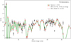 |
Fig. 8 Model fit using starfit for the abundances of TYC 9219-2422-1. The dashed line is a model from the DB0 database of pop III progenitor stars from Heger & Woosley (2010) and later updates. The dash-dotted line is a model from the DB3 database of NSM r-process models from Mendoza-Temis et al. (2015) and Wu et al. (2016). Model 33, which best fits the neutron-capture abundances here, is a NSM model that forms a black hole of about 3M⊙ with a torus ejecta of 0.10M⊙ (for more details see model m0.10 in Wu et al. 2016). The black points are the observed abundances. The green line with red triangles is the sum of the two best-fitting models. |
 |
Fig. 9 Model fit using starfit for the abundances for BPS CS 29529-0089. The dashed line is a model from the DB0 database of pop III progenitor stars from Heger & Woosley (2010) and later updates. The dash-dotted line is a model from the DB3 database of NSM r-process models from Mendoza-Temis et al. (2015) and Wu et al. (2016). Model 19, which best fits the neutron-capture abundances here, is a NSM model that forms a black hole of about 3M⊙ with a torus eject of 0.03M⊙ (for more details see the similar model S-def in Wu et al. 2016). The black points are the observed abundances. The green line with red triangles is the sum of the two best-fitting models. |
5 Conclusions
In this work, we present the chemical abundance analysis of BPS CS 29529-0089, TYC 9219-2422-1 ,and HD 122563 using highresolution spectra obtained with the UVES spectrograph. Atmospheric parameters were determined iteratively using IRFM calibrations, bolometric corrections, Gaia parallaxes, and Fe II lines. We also determined abundances for 47 chemical species of 44 elements through spectral grid generation. Corrections for departures from LTE were used for 15 chemical species of 13 elements. We investigated the chemodynamics of the stars following the procedure outlined in da Silva & Smiljanic (2023), to investigate the possible origins of the objects in the Milky Way evolution context. We find that their abundances of C, Mg, Ni, Sc, Mn, and Al are consistent with expectations for mono-enriched stars, following Hartwig et al. (2018, see their Fig. 18).
BPS CS 29529-0089 has enhanced abundances of a series of elements produced by neutron-capture processes. This made possible the determination of an almost complete set of heavy elements with lines available between 330 nm to 670 nm. We found that BPS CS 29529-0089 is the first known r-II star ([Eu/Fe] = +1.79 dex) with thick disk dynamics that is not carbon-enhanced. Two other r-II stars in the MWTD are known, but they are both CEMP. We suggest that the most probably BPS CS 29529-0089 was formed in situ, in the proto-disk of the Milky Way. Alongside other thick disk stars, its kinematics was probably heated during the merger events undergone by the Milky Way, such as the one with Gaia-Sausage-Enceladus. The abundance pattern of BPS CS 29529-0089 could be explained by the combination of two phenomena: i) for elements with Z ≤ 30 (until Zn), a supernova of a pop III progenitor with 15 M⊙ , and ii) for elements with Z ≥ 38 (from Sr), a NSM r-process enrichment that happened about 13 Ga ago. We speculate that fission products could explain some of the excesses of neutroncapture elements seen around Z ∼ 40 and 58, in the same way as is discussed in Roederer et al. (2024).
TYC 9219-2422-1 is an archetypal star from Gaia-Sausage- Enceladus. It has a moderate europium enrichment of [Eu/Fe] = +0.54(17) dex with [Ba/Fe] = −0.16(12), which leads to the r-I classification. The [Eu/Mg] ratio observed in TYC 9219-24221 is also in agreement with the range observed for the Gaia- Sausage-Enceladus magnesium-poor tail (Matsuno et al. 2021; Ou et al. 2024). The orbit of TYC 9219-2422-1, although slightly prograde, is highly eccentric, e ~ 0.8, which agrees with the well-known high eccentricity of Gaia-Sausage-Enceladus (see e.g., Helmi 2008; Koppelman et al. 2020; Limberg et al. 2021; da Silva & Smiljanic 2023). The TYC 9219-2422-1abundance pattern could be explained by the combination of two phenomena: i) for elements with Z ≤ 30 (until Zn), a supernova of a pop III progenitor with 10.7 M⊙, and ii) for elements with Z ≥ 38 (from Sr), a NSM r-process enrichment that happened about 13 Ga ago.
HD 122563 was in principle also found to be associated with Gaia-Sausage-Enceladus, based on the values of actions, [Fe/H], and [Mg/Fe]. However, this star has very low abundances of neutron capture elements. This pattern does not match the established Gaia-Sausage-Enceladus r-process enrichment (Aguado et al. 2021; Matsuno et al. 2021). Therefore, most probably HD 122563 is an old metal-poor in situ halo star.
Data availability
A list of lines, log gf, and abundances are provided in Zenodo
Acknowledgements
ARS and RS acknowledge the support of the Polish National Science Centre (NCN) through the project 2018/31/B/ST9/01469. ARS thanks Riano Giribaldi for the discussion on HD122563 and the data provided. ARS thanks Hélio Perottoni, Maria L. L. Dantas and Guilherme Limberg for the discussions. This work is based on observations collected at the European Southern Observatory under ESO programmes: 0108.D-0626(A) and 65.L-0507. This research has made use of the SIMBAD database, operated at CDS, Strasbourg, France and of NASA’s Astrophysics Data System. This research has made use of the NASA/IPAC Infrared Science Archive, which is funded by the National Aeronautics and Space Administration and operated by the California Institute of Technology. This work has made use of data from the European Space Agency (ESA) mission Gaia (https://www.cosmos.esa.int/gaia), processed by the Gaia Data Processing and Analysis Consortium (DPAC, https://www.cosmos.esa.int/web/gaia/dpac/consortium). Funding for the DPAC has been provided by national institutions, in particular the institutions participating in the Gaia Multilateral Agreement. This work also made use of GALAH survey data, their website is http://galah-survey.org/.
Appendix A Chemical abundances and dynamics
Tables with the determined chemical abundances and dynamic parameters are available in tables A.1 and A.2.
Appendix B Hyperfine structure and isotopic splitting of the Eu II lines
This appendix lists the oscillator strengths for each hyperfine component of the Eu II lines that were analyzed in this work, for the two isotopes of importance that were considered here. The isotopic fractions (47.81% and 52.19%, for A = 151 and A = 153, respectively) are taken into account as an additional multiplicative factor internally to the spectrum synthesis.
Appendix C Hyperfine structure and isotopic splitting of the Ba II lines
This appendix lists the oscillator strengths for the isotopic splitting of the Ba II lines, and their hyperfine components when relevant. The isotopic fractions (2.417%, 6.592%, 7.854%, 11.232%, and 71.698%, for A = 134, 135, 136, 137, and 138, respectively) are taken into account as an additional multiplicative factor internally to the spectrum synthesis.
Appendix D Line fits
On this appendix, we provide some line fits using the observed spectra and the synthetic fit with determined abundances. We provide the the fits for the carbon-band from 429 to 431 nm in Fig. D.1. Barium lines in Fig. D.2. Europium lines in Fig. D.3. Thorium lines in Figs. D.4 and D.5. Molybdenum in Fig. D.6. For BPS CS 29529-0089 some other interesting element lines in Figs. Os: D.7, Yb: D.8, Ce: D.9, Nd: D.10 and Sr: D.11.
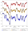 |
Fig. D.1 Molecular band of CH from 4307 to 4310 Å for BPS CS 29529-0089, TYC 9219-2422-1 and HD 122563 with fit abundance and ±0.2 dex. |
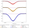 |
Fig. D.2 Ba line in 6141 Å for BPS CS 29529-0089, TYC 9219-24221 and HD 122563 with fit abundance and ±0.2 dex. Fluxes are offset by 0.5. BPS CS 29529-0089 is shown in blue, TYC 9219-2422-1 in orange and HD 122563 in red. |
Determined abundances and uncertainties
Kinematic and dynamic parameters
Hyperfine structure of the Eu II line at 3724.9 Å.
Hyperfine structure of the Eu II line at 3819.6 Å.
Hyperfine structure of the Eu II line at 3907.1 Å.
Hyperfine structure of the Eu II line at 3930.5 Å.
Hyperfine structure of the Eu II line at 4129.7 Å.
Hyperfine structure of the Eu II line at 4205.0 Å.
Hyperfine structure of the Eu II line at 6645.1 Å.
Isotopic splitting and HFS of the Ba II line at 5853.675 Å.
Isotopic splitting and HFS of the Ba II line at 6141.71 Å.
Isotopic splitting and HFS of the Ba II line at 6496.69 Å.
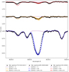 |
Fig. D.3 Eu line in 4129 Å for BPS CS 29529-0089, TYC 9219-2422-1 and HD 122563 with fit abundance and ±0.2 dex. Fluxes are offset by 0.5. BPS CS 29529-0089 is shown in blue, TYC 9219-2422-1 in orange and HD 122563 in red. |
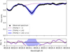 |
Fig. D.4 Th line 4019 Å for BPS CS 29529-0089 with best fit abundance for the line and ±0.2 dex. |
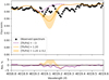 |
Fig. D.5 Th line 4019 Å for TYC 9219-2422-1 with upper limit and ±0.2 dex. |
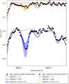 |
Fig. D.6 Mo line 3864 Å for BPS CS 29529-0089 and TYC 9219-2422-1 with fit abundance and ±0.2 dex. Fluxes are offset by 0.2. |
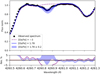 |
Fig. D.7 Os line in 4260 Å for BPS CS 29529-0089 with fit abundance and ±0.2 dex. |
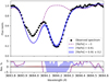 |
Fig. D.8 Yb line 3694 Å for BPS CS 29529-0089 with fit abundance and ±0.2 dex. |
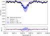 |
Fig. D.9 Ce line 5187 Å for BPS CS 29529-0089 with fit abundance and ±0.2 dex. |
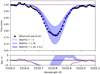 |
Fig. D.10 Nd line 5319 Å for BPS CS 29529-0089 with fit abundance and ±0.2 dex. |
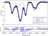 |
Fig. D.11 Sr line 4078 Å for BPS CS 29529-0089 with fit abundance and ±0.2 dex. |
References
- Abbott, B. P., Abbott, R., Abbott, T. D., et al. 2017, Phys. Rev. Lett., 119, 161101 [Google Scholar]
- Abohalima, A., & Frebel, A. 2018, ApJS, 238, 36 [NASA ADS] [CrossRef] [Google Scholar]
- Aguado, D. S., Belokurov, V., Myeong, G. C., et al. 2021, ApJ, 908, L8 [NASA ADS] [CrossRef] [Google Scholar]
- Allen, D. M., Ryan, S. G., Rossi, S., Beers, T. C., & Tsangarides, S. A. 2012, A&A, 548, A34 [NASA ADS] [CrossRef] [EDP Sciences] [Google Scholar]
- Arcones, A., & Thielemann, F.-K. 2023, A&A Rev., 31, 1 [NASA ADS] [CrossRef] [Google Scholar]
- Asplund, M., Grevesse, N., Sauval, A. J., & Scott, P. 2009, ARA&A, 47, 481 [NASA ADS] [CrossRef] [Google Scholar]
- Bagnulo, S., Jehin, E., Ledoux, C., et al. 2003, The Messenger, 114, 10 [Google Scholar]
- Ballester, P., Modigliani, A., Boitquin, O., et al. 2000, The Messenger, 101, 31 [NASA ADS] [Google Scholar]
- Barbuy, B., Meléndez, J., Spite, M., et al. 2003, ApJ, 588, 1072 [NASA ADS] [CrossRef] [Google Scholar]
- Bartos, I., & Marka, S. 2019, Nature, 569, 85 [Google Scholar]
- Beers, T. C., & Christlieb, N. 2005, ARA&A, 43, 531 [NASA ADS] [CrossRef] [Google Scholar]
- Beers, T. C., Drilling, J. S., Rossi, S., et al. 2002, AJ, 124, 931 [CrossRef] [Google Scholar]
- Belokurov, V., Erkal, D., Evans, N. W., Koposov, S. E., & Deason, A. J. 2018, MNRAS, 478, 611 [Google Scholar]
- Bergemann, M. 2011, MNRAS, 413, 2184 [NASA ADS] [CrossRef] [Google Scholar]
- Bergemann, M., Pickering, J. C., & Gehren, T. 2010, MNRAS, 401, 1334 [CrossRef] [Google Scholar]
- Bergemann, M., Hansen, C. J., Bautista, M., & Ruchti, G. 2012, A&A, 546, A90 [NASA ADS] [CrossRef] [EDP Sciences] [Google Scholar]
- Bergemann, M., Collet, R., Amarsi, A. M., et al. 2017, ApJ, 847, 15 [NASA ADS] [CrossRef] [Google Scholar]
- Bergemann, M., Gallagher, A. J., Eitner, P., et al. 2019, A&A, 631, A80 [NASA ADS] [CrossRef] [EDP Sciences] [Google Scholar]
- Bergemann, M., Hoppe, R., Semenova, E., et al. 2021, MNRAS, 508, 2236 [NASA ADS] [CrossRef] [Google Scholar]
- Bisterzo, S., Travaglio, C., Gallino, R., Wiescher, M., & Käppeler, F. 2014, ApJ, 787, 10 [NASA ADS] [CrossRef] [Google Scholar]
- Blanchard, P. K., Villar, V. A., Chornock, R., et al. 2024, Nat. Astron., 8, 774 [NASA ADS] [CrossRef] [Google Scholar]
- Blanco-Cuaresma, S. 2019, MNRAS, 486, 2075 [Google Scholar]
- Blanco-Cuaresma, S., Soubiran, C., Heiter, U., & Jofré, P. 2014, A&A, 569, A111 [CrossRef] [EDP Sciences] [Google Scholar]
- Bonifacio, P., Caffau, E., Monaco, L., et al. 2024, A&A, 684, A91 [NASA ADS] [CrossRef] [EDP Sciences] [Google Scholar]
- Bovy, J. 2015, ApJS, 216, 29 [NASA ADS] [CrossRef] [Google Scholar]
- Buder, S., Sharma, S., Kos, J., et al. 2021, MNRAS, 506, 150 [NASA ADS] [CrossRef] [Google Scholar]
- Burbidge, E. M., Burbidge, G. R., Fowler, W. A., & Hoyle, F. 1957, Rev. Mod. Phys., 29, 547 [NASA ADS] [CrossRef] [Google Scholar]
- Cain, M., Frebel, A., Ji, A. P., et al. 2020, ApJ, 898, 40 [NASA ADS] [CrossRef] [Google Scholar]
- Casagrande, L., Lin, J., Rains, A. D., et al. 2021, MNRAS, 507, 2684 [NASA ADS] [CrossRef] [Google Scholar]
- Cayrel, R., Hill, V., Beers, T. C., et al. 2001, Nature, 409, 691 [CrossRef] [PubMed] [Google Scholar]
- Cenarro, A. J., Moles, M., Cristóbal-Hornillos, D., et al. 2019, A&A, 622, A176 [NASA ADS] [CrossRef] [EDP Sciences] [Google Scholar]
- Cescutti, G., Bonifacio, P., Caffau, E., et al. 2022, A&A, 668, A168 [NASA ADS] [CrossRef] [EDP Sciences] [Google Scholar]
- Choplin, A., Siess, L., & Goriely, S. 2023, in European Physical Journal Web of Conferences, 279, 07001 [NASA ADS] [CrossRef] [EDP Sciences] [Google Scholar]
- Coulter, D. A., Foley, R. J., Kilpatrick, C. D., et al. 2017, Science, 358, 1556 [NASA ADS] [CrossRef] [Google Scholar]
- Cowan, J. J., Sneden, C., Lawler, J. E., et al. 2021, Rev. Mod. Phys., 93, 015002 [Google Scholar]
- Da Costa, G. S., Bessell, M. S., Nordlander, T., et al. 2023, MNRAS, 520, 917 [NASA ADS] [CrossRef] [Google Scholar]
- da Silva, A. R., & Smiljanic, R. 2023, A&A, 677, A74 [NASA ADS] [CrossRef] [EDP Sciences] [Google Scholar]
- Das, P., Hawkins, K., & Jofré, P. 2020, MNRAS, 493, 5195 [NASA ADS] [CrossRef] [Google Scholar]
- Deka-Szymankiewicz, B., Niedzielski, A., Adamczyk, M., et al. 2018, A&A, 615, A31 [NASA ADS] [CrossRef] [EDP Sciences] [Google Scholar]
- Dekker, H., D’Odorico, S., Kaufer, A., Delabre, B., & Kotzlowski, H. 2000, SPIE Conf. Ser., 4008, 534 [Google Scholar]
- De Silva, G. M., Freeman, K. C., Bland-Hawthorn, J., et al. 2015, MNRAS, 449, 2604 [NASA ADS] [CrossRef] [Google Scholar]
- Domoto, N., Tanaka, M., Wanajo, S., & Kawaguchi, K. 2021, ApJ, 913, 26 [NASA ADS] [CrossRef] [Google Scholar]
- Domoto, N., Tanaka, M., Kato, D., et al. 2022, ApJ, 939, 8 [NASA ADS] [CrossRef] [Google Scholar]
- Donlon, T., Newberg, H. J., Sanderson, R., et al. 2024, MNRAS, 531, 1422 [NASA ADS] [CrossRef] [Google Scholar]
- Emery, G. 2006, in Springer Handbook of Atomic, ed. G. W. F. Drake (Springer), 253 [CrossRef] [Google Scholar]
- Ernandes, H., Barbuy, B., Friaça, A., et al. 2022, MNRAS, 510, 5362 [CrossRef] [Google Scholar]
- Ernandes, H., Castro, M. J., Barbuy, B., et al. 2023, MNRAS, 524, 656 [NASA ADS] [CrossRef] [Google Scholar]
- Ernandes, H., Feuillet, D., Feltzing, S., & Skúladóttir, Á. 2024, A&A, 691, A333 [NASA ADS] [CrossRef] [EDP Sciences] [Google Scholar]
- Ezzeddine, R., Merle, T., Plez, B., et al. 2018, A&A, 618, A141 [NASA ADS] [CrossRef] [EDP Sciences] [Google Scholar]
- Ezzeddine, R., Rasmussen, K., Frebel, A., et al. 2020, ApJ, 898, 150 [NASA ADS] [CrossRef] [Google Scholar]
- Forsberg, R., Rich, R. M., Nieuwmunster, N., et al. 2023, A&A, 669, A17 [Google Scholar]
- François, P., Depagne, E., Hill, V., et al. 2007, A&A, 476, 935 [Google Scholar]
- François, P., Cescutti, G., Bonifacio, P., et al. 2024, A&A, 686, A295 [NASA ADS] [CrossRef] [EDP Sciences] [Google Scholar]
- Frebel, A., & Norris, J. E. 2015, ARA&A, 53, 631 [NASA ADS] [CrossRef] [Google Scholar]
- Gaia Collaboration (Prusti, T., et al.) 2016, A&A, 595, A1 [NASA ADS] [CrossRef] [EDP Sciences] [Google Scholar]
- Gaia Collaboration (Brown, A. G. A., et al.) 2021, A&A, 649, A1 [NASA ADS] [CrossRef] [EDP Sciences] [Google Scholar]
- Gallagher, A. J., Bergemann, M., Collet, R., et al. 2020, A&A, 634, A55 [NASA ADS] [CrossRef] [EDP Sciences] [Google Scholar]
- Gerber, J. M., Magg, E., Plez, B., et al. 2023, A&A, 669, A43 [NASA ADS] [CrossRef] [EDP Sciences] [Google Scholar]
- Gillanders, J. H., McCann, M., Sim, S. A., Smartt, S. J., & Ballance, C. P. 2021, MNRAS, 506, 3560 [NASA ADS] [CrossRef] [Google Scholar]
- Giribaldi, R. E., & Smiljanic, R. 2023a, Exp. Astron., 55, 117 [NASA ADS] [CrossRef] [Google Scholar]
- Giribaldi, R. E., & Smiljanic, R. 2023b, A&A, 673, A18 [NASA ADS] [CrossRef] [EDP Sciences] [Google Scholar]
- Giribaldi, R. E., da Silva, A. R., Smiljanic, R., & Cornejo Espinoza, D. 2021, A&A, 650, A194 [NASA ADS] [CrossRef] [EDP Sciences] [Google Scholar]
- Giribaldi, R. E., Van Eck, S., Merle, T., et al. 2023, A&A, 679, A110 [NASA ADS] [CrossRef] [EDP Sciences] [Google Scholar]
- Goswami, P. P., Rathour, R. S., & Goswami, A. 2021, A&A, 649, A49 [NASA ADS] [CrossRef] [EDP Sciences] [Google Scholar]
- Gudin, D., Shank, D., Beers, T. C., et al. 2021, ApJ, 908, 79 [NASA ADS] [CrossRef] [Google Scholar]
- Gustafsson, B., Edvardsson, B., Eriksson, K., et al. 2008, A&A, 486, 951 [NASA ADS] [CrossRef] [EDP Sciences] [Google Scholar]
- Hanke, M., Hansen, C. J., Ludwig, H.-G., et al. 2020, A&A, 635, A104 [NASA ADS] [CrossRef] [EDP Sciences] [Google Scholar]
- Hansen, T. T., Ji, A. P., Da Costa, G. S., et al. 2021, ApJ, 915, 103 [NASA ADS] [CrossRef] [Google Scholar]
- Hartwig, T., Yoshida, N., Magg, M., et al. 2018, MNRAS, 478, 1795 [CrossRef] [Google Scholar]
- Heger, A., & Woosley, S. E. 2010, ApJ, 724, 341 [Google Scholar]
- Heiter, U., Lind, K., Bergemann, M., et al. 2021, A&A, 645, A106 [EDP Sciences] [Google Scholar]
- Helmi, A. 2008, A&A Rev., 15, 145 [NASA ADS] [CrossRef] [Google Scholar]
- Helmi, A., Babusiaux, C., Koppelman, H. H., et al. 2018, Nature, 563, 85 [Google Scholar]
- Hill, V., Plez, B., Cayrel, R., et al. 2002, A&A, 387, 560 [CrossRef] [EDP Sciences] [Google Scholar]
- Hirai, Y., Beers, T. C., Chiba, M., et al. 2022, MNRAS, 517, 4856 [NASA ADS] [CrossRef] [Google Scholar]
- Hirai, Y., Beers, T. C., Lee, Y. S., et al. 2024, arXiv e-prints [arXiv:2410.11943] [Google Scholar]
- Holmbeck, E. M., Beers, T. C., Roederer, I. U., et al. 2018, ApJ, 859, L24 [NASA ADS] [CrossRef] [Google Scholar]
- Holmbeck, E. M., Hansen, T. T., Beers, T. C., et al. 2020, ApJS, 249, 30 [NASA ADS] [CrossRef] [Google Scholar]
- Honda, S., Aoki, W., Ishimaru, Y., Wanajo, S., & Ryan, S. G. 2006, ApJ, 643, 1180 [NASA ADS] [CrossRef] [Google Scholar]
- Hotokezaka, K., Tanaka, M., Kato, D., & Gaigalas, G. 2023, MNRAS, 526, L155 [NASA ADS] [CrossRef] [Google Scholar]
- Hou, X., Zhao, G., & Li, H. 2024, MNRAS, 532, 1099 [NASA ADS] [CrossRef] [Google Scholar]
- Ji, A. P., Frebel, A., Simon, J. D., & Chiti, A. 2016, ApJ, 830, 93 [NASA ADS] [CrossRef] [Google Scholar]
- Jofré, P., Heiter, U., Soubiran, C., et al. 2014, A&A, 564, A133 [NASA ADS] [CrossRef] [EDP Sciences] [Google Scholar]
- Johnson, C. I., McWilliam, A., & Rich, R. M. 2013, ApJ, 775, L27 [NASA ADS] [CrossRef] [Google Scholar]
- Koppelman, H. H., Helmi, A., Massari, D., Price-Whelan, A. M., & Starkenburg, T. K. 2019, A&A, 631, L9 [NASA ADS] [CrossRef] [EDP Sciences] [Google Scholar]
- Koppelman, H. H., Bos, R. O. Y., & Helmi, A. 2020, A&A, 642, L18 [NASA ADS] [CrossRef] [EDP Sciences] [Google Scholar]
- Kratz, K.-L., Farouqi, K., Pfeiffer, B., et al. 2007, ApJ, 662, 39 [NASA ADS] [CrossRef] [Google Scholar]
- Lattimer, J. M., & Schramm, D. N. 1974, ApJ, 192, L145 [NASA ADS] [CrossRef] [Google Scholar]
- Lawler, J. E., Wickliffe, M. E., den Hartog, E. A., & Sneden, C. 2001, ApJ, 563, 1075 [CrossRef] [Google Scholar]
- Li, L.-X., & Paczyński, B. 1998, ApJ, 507, L59 [NASA ADS] [CrossRef] [Google Scholar]
- Limberg, G., Rossi, S., Beers, T. C., et al. 2021, ApJ, 907, 10 [Google Scholar]
- Limberg, G., Ji, A. P., Naidu, R. P., et al. 2024, MNRAS, 530, 2512 [NASA ADS] [CrossRef] [Google Scholar]
- Lindegren, L., Bastian, U., Biermann, M., et al. 2021, A&A, 649, A4 [EDP Sciences] [Google Scholar]
- Ludwig, H. G., Caffau, E., Steffen, M., Bonifacio, P., & Sbordone, L. 2010, A&A, 509, A84 [NASA ADS] [CrossRef] [EDP Sciences] [Google Scholar]
- Lugaro, M., Pignatari, M., Reifarth, R., & Wiescher, M. 2023, Annu. Rev. Nucl. Part. Sci., 73, 315 [NASA ADS] [CrossRef] [Google Scholar]
- Magg, E., Bergemann, M., Serenelli, A., et al. 2022, A&A, 661, A140 [NASA ADS] [CrossRef] [EDP Sciences] [Google Scholar]
- Majewski, S. R., APOGEE Team, & APOGEE-2 Team 2016, Astron. Nachr., 337, 863 [NASA ADS] [CrossRef] [Google Scholar]
- Masana, E., Jordi, C., & Ribas, I. 2006, A&A, 450, 735 [NASA ADS] [CrossRef] [EDP Sciences] [Google Scholar]
- Mashonkina, L., Sitnova, T., & Belyaev, A. K. 2017, A&A, 605, A53 [NASA ADS] [CrossRef] [EDP Sciences] [Google Scholar]
- Mashonkina, L., Arentsen, A., Aguado, D. S., et al. 2023, MNRAS, 523, 2111 [NASA ADS] [CrossRef] [Google Scholar]
- Mathar, R. J. 2011, J. Phys. A: Math. Gen. 37, 3259 [Google Scholar]
- Matsuno, T., Hirai, Y., Tarumi, Y., et al. 2021, A&A, 650, A110 [NASA ADS] [CrossRef] [EDP Sciences] [Google Scholar]
- McMillan, P. J. 2017, MNRAS, 465, 76 [NASA ADS] [CrossRef] [Google Scholar]
- Meléndez, J., & Barbuy, B. 2009, A&A, 497, 611 [NASA ADS] [CrossRef] [EDP Sciences] [Google Scholar]
- Mendes de Oliveira, C., Ribeiro, T., Schoenell, W., et al. 2019, MNRAS, 489, 241 [NASA ADS] [CrossRef] [Google Scholar]
- Mendoza-Temis, J. D. J., Wu, M.-R., Langanke, K., et al. 2015, Phys. Rev. C, 92, 055805 [CrossRef] [Google Scholar]
- Monty, S., Belokurov, V., Sanders, J. L., et al. 2024, MNRAS, 533, 2420 [NASA ADS] [CrossRef] [Google Scholar]
- Mucciarelli, A., Monaco, L., Bonifacio, P., et al. 2022, A&A, 661, A153 [NASA ADS] [CrossRef] [EDP Sciences] [Google Scholar]
- Myeong, G. C., Vasiliev, E., Iorio, G., Evans, N. W., & Belokurov, V. 2019, MNRAS, 488, 1235 [Google Scholar]
- Nordlander, T., & Lind, K. 2017, A&A, 607, A75 [NASA ADS] [CrossRef] [EDP Sciences] [Google Scholar]
- Ou, X., Ji, A. P., Frebel, A., Naidu, R. P., & Limberg, G. 2024, ApJ, 974, 232 [NASA ADS] [CrossRef] [Google Scholar]
- Perottoni, H. D., Placco, V. M., Almeida-Fernandes, F., et al. 2024, A&A, 691, A138 [NASA ADS] [CrossRef] [EDP Sciences] [Google Scholar]
- Pian, E., D’Avanzo, P., Benetti, S., et al. 2017, Nature, 551, 67 [Google Scholar]
- Placco, V. M., Frebel, A., Beers, T. C., & Stancliffe, R. J. 2014, ApJ, 797, 21 [Google Scholar]
- Placco, V. M., Sneden, C., Roederer, I. U., et al. 2021, RNAAS, 5, 92 [NASA ADS] [Google Scholar]
- Placco, V. M., Almeida-Fernandes, F., Holmbeck, E. M., et al. 2023, ApJ, 959, 60 [NASA ADS] [CrossRef] [Google Scholar]
- Plez, B. 2012, Turbospectrum: Code for spectral synthesis, Astrophysics Source Code Library [record ascl:1205.004] [Google Scholar]
- Purandardas, M., Goswami, A., Goswami, P. P., Shejeelammal, J., & Masseron, T. 2019, MNRAS, 486, 3266 [Google Scholar]
- Randich, S., Gilmore, G., Magrini, L., et al. 2022, A&A, 666, A121 [NASA ADS] [CrossRef] [EDP Sciences] [Google Scholar]
- Reggiani, H., Schlaufman, K. C., Casey, A. R., Simon, J. D., & Ji, A. P. 2021, AJ, 162, 229 [NASA ADS] [CrossRef] [Google Scholar]
- Reichert, M., Hansen, C. J., Hanke, M., et al. 2020, A&A, 641, A127 [NASA ADS] [CrossRef] [EDP Sciences] [Google Scholar]
- Reichert, M., Hansen, C. J., & Arcones, A. 2021, ApJ, 912, 157 [NASA ADS] [CrossRef] [Google Scholar]
- Riello, M., De Angeli, F., Evans, D. W., et al. 2021, A&A, 649, A3 [NASA ADS] [CrossRef] [EDP Sciences] [Google Scholar]
- Roederer, I. U., Hattori, K., & Valluri, M. 2018a, AJ, 156, 179 [NASA ADS] [CrossRef] [Google Scholar]
- Roederer, I. U., Sakari, C. M., Placco, V. M., et al. 2018b, ApJ, 865, 129 [NASA ADS] [CrossRef] [Google Scholar]
- Roederer, I. U., Lawler, J. E., Den Hartog, E. A., et al. 2022, ApJS, 260, 27 [NASA ADS] [CrossRef] [Google Scholar]
- Roederer, I. U., Vassh, N., Holmbeck, E. M., et al. 2023, Science, 382, 1177 [CrossRef] [PubMed] [Google Scholar]
- Roederer, I. U., Beers, T. C., Hattori, K., et al. 2024, ApJ, 971, 158 [NASA ADS] [CrossRef] [Google Scholar]
- Ryabchikova, T., Piskunov, N., Kurucz, R. L., et al. 2015, Phys. Scr, 90, 054005 [Google Scholar]
- Saraf, P., Allende Prieto, C., Sivarani, T., et al. 2023, MNRAS, 524, 5607 [NASA ADS] [CrossRef] [Google Scholar]
- Schatz, H., Toenjes, R., Pfeiffer, B., et al. 2002, ApJ, 579, 626 [NASA ADS] [CrossRef] [Google Scholar]
- Schlafly, E. F., & Finkbeiner, D. P. 2011, ApJ, 737, 103 [Google Scholar]
- Sestito, F., Hayes, C. R., Venn, K. A., et al. 2024, MNRAS, 528, 4838 [NASA ADS] [CrossRef] [Google Scholar]
- Shah, S. P., Ezzeddine, R., Roederer, I. U., et al. 2024, MNRAS, 529, 1917 [NASA ADS] [CrossRef] [Google Scholar]
- Shank, D., Beers, T. C., Placco, V. M., et al. 2022a, ApJ, 926, 26 [NASA ADS] [CrossRef] [Google Scholar]
- Shank, D., Komater, D., Beers, T. C., Placco, V. M., & Huang, Y. 2022b, ApJS, 261, 19 [NASA ADS] [CrossRef] [Google Scholar]
- Shank, D., Beers, T. C., Placco, V. M., et al. 2023, ApJ, 943, 23 [NASA ADS] [CrossRef] [Google Scholar]
- Siegel, D. M. 2019, Eur. Phys. J. A, 55, 203 [NASA ADS] [CrossRef] [Google Scholar]
- Siqueira Mello, C., Hill, V., Barbuy, B., et al. 2014, A&A, 565, A93 [NASA ADS] [CrossRef] [EDP Sciences] [Google Scholar]
- Skrutskie, M. F., Cutri, R. M., Stiening, R., et al. 2006, AJ, 131, 1163 [NASA ADS] [CrossRef] [Google Scholar]
- Smiljanic, R., da Silva, A. R., & Giribaldi, R. E. 2023, Exp. Astron., 55, 95 [NASA ADS] [CrossRef] [Google Scholar]
- Smith, B. D., Wise, J. H., O’Shea, B. W., Norman, M. L., & Khochfar, S. 2015, MNRAS, 452, 2822 [Google Scholar]
- Sneden, C., Preston, G. W., McWilliam, A., & Searle, L. 1994, ApJ, 431, L27 [NASA ADS] [CrossRef] [Google Scholar]
- Sneden, C., Cowan, J. J., & Gallino, R. 2008, ARA&A, 46, 241 [Google Scholar]
- Soubiran, C., Creevey, O. L., Lagarde, N., et al. 2024, A&A, 682, A145 [NASA ADS] [CrossRef] [EDP Sciences] [Google Scholar]
- Spite, F., & Spite, M. 1982, A&A, 115, 357 [NASA ADS] [Google Scholar]
- Storm, N., & Bergemann, M. 2023, MNRAS, 525, 3718 [NASA ADS] [CrossRef] [Google Scholar]
- Suda, T., Katsuta, Y., Yamada, S., et al. 2008, PASJ, 60, 1159 [NASA ADS] [Google Scholar]
- Symbalisty, E., & Schramm, D. N. 1982, Astrophys. Lett., 22, 143 [NASA ADS] [Google Scholar]
- Tanvir, N. R., Levan, A. J., González-Fernández, C., et al. 2017, ApJ, 848, L27 [CrossRef] [Google Scholar]
- Valenti, S., Sand, D. J., Yang, S., et al. 2017, ApJ, 848, L24 [CrossRef] [Google Scholar]
- Van Hove, M., Borghs, G., DeBisschop, P., & Silverans, R. E. 1982, J. Phys. B At. Mol. Phys., 15, 1805 [NASA ADS] [CrossRef] [Google Scholar]
- Vieira, N., Ruan, J. J., Haggard, D., et al. 2024, ApJ, 962, 33 [NASA ADS] [CrossRef] [Google Scholar]
- Villemoes, P., Arnesen, A., Heijkenskjold, F., & Wannstrom, A. 1993, J. Phys. B At. Mol. Phys., 26, 4289 [NASA ADS] [CrossRef] [Google Scholar]
- Virtanen, P., Gommers, R., Oliphant, T. E., et al. 2020, Nat. Methods, 17, 261 [Google Scholar]
- Viswanathan, A., Starkenburg, E., Matsuno, T., et al. 2024, A&A, 683, L11 [NASA ADS] [CrossRef] [EDP Sciences] [Google Scholar]
- Watson, D., Hansen, C. J., Selsing, J., et al. 2019, Nature, 574, 497 [NASA ADS] [CrossRef] [Google Scholar]
- Wu, M.-R., Fernández, R., Martínez-Pinedo, G., & Metzger, B. D. 2016, MNRAS, 463, 2323 [NASA ADS] [CrossRef] [Google Scholar]
- Xie, X.-J., Shi, J., Yan, H.-L., et al. 2024, ApJ, 970, L30 [NASA ADS] [CrossRef] [Google Scholar]
- Xing, Q., Zhao, G., Aoki, W., et al. 2024, ApJ, 965, 79 [NASA ADS] [CrossRef] [Google Scholar]
- Xylakis-Dornbusch, T., Christlieb, N., Hansen, T. T., et al. 2024, A&A, 687, A177 [NASA ADS] [CrossRef] [EDP Sciences] [Google Scholar]
- Yuan, Z., Myeong, G. C., Beers, T. C., et al. 2020, ApJ, 891, 39 [NASA ADS] [CrossRef] [Google Scholar]
- Zacharias, N., Finch, C. T., Girard, T. M., et al. 2013, AJ, 145, 44 [Google Scholar]
We adopt the SI standard for uncertainties throughout the text. In this notation, the numbers in parenthesis are uncertainties in the last digits of the number, i.e. 3.11(1) is equivalent to 3.11 ± 0.01 while 3.1(1) is equivalent to 3.1 ± 0.1.
Giribaldi, R. 2024, private communication.
The lower-case letter ‘a’ is the symbol adopted by the International Astronomical Union (IAU) and the bureau of weights and measures of the International System of Units (BIPM/SI) for ‘year’, and is thus the symbol used here.
Using calculator available in http://vplacco.pythonanywhere.com/
Available in https://jinabase.pythonanywhere.com/
 and
and  are the axis of the Action Map, we use a system that Jϕ=Lz.
All Tables
All Figures
|
Fig. 1 Selection of anomalous stars in GALAH DR3. In gray scale is a 2D histogram of all stars in GALAH DR3 with Ba and Eu abundances. The red ellipsis marks the region differing by 3 σ from the mean abundances. The red star symbols show the anomalous stars that also have [Fe/H] ≤ 2. The two stars analyzed here are shown in different colors. |
| In the text | |
|
Fig. 2 The [Eu/Fe] ratio as a function of [Fe/H]. The stars shown as circles are non-CEMP metal-poor stars from the JINA database (Abohalima & Frebel 2018). Open circles are ordinary stars, while brown ones are RPEs. R-I, r-II, and r-III levels are shown by the red lines. BPS CS 29529-0089 and TYC 9219-2422-1 are shown as colored star symbols. |
| In the text | |
|
Fig. 3 Projection map obtained using t-SNE. The gray stars are the sample from GALAH used in da Silva & Smiljanic (2023). The four groups defined in that work (Gaia Enceladus, prograde, retrograde, and most retrograde) are colored in green, blue, light brown, and dark purple, respectively. The cyan stars are 28 RPE stars with [Eu/Fe] ≥ + 1.7 dex found in the SAGA database (Soubiran et al. 2024) complemented by five stars from Roederer et al. (2024). The Sun is added as reference. |
| In the text | |
|
Fig.4 Lindblad diagram (Lz × En). Coloring is the same as Fig. 3. Error bars are smaller than the size of the symbols. |
| In the text | |
|
Fig. 5 Action map. Coloring is the same as Fig. 3. Note BPS CS 29529- 0089in the most prograde, circular and in the plane orbits. Error bars are smaller than the size of the symbols. |
| In the text | |
|
Fig. 6 Top: comparison of the solar r-process abundance pattern with the abundances of BPS CS 29529-0089. Bottom: same comparison for TYC 9219-2422-1. |
| In the text | |
|
Fig. 7 [Mg/H] by [Eu/Mg] plane. Black circles are stars from Ou et al. (2024), green squares are stars from MINCE (Cescutti et al. 2022; François et al. 2024, as cited in Ou et al. 2024), and blue triangles are stars from Aguado et al. (2021). TYC 9219-2422-1 is the orange star. |
| In the text | |
|
Fig. 8 Model fit using starfit for the abundances of TYC 9219-2422-1. The dashed line is a model from the DB0 database of pop III progenitor stars from Heger & Woosley (2010) and later updates. The dash-dotted line is a model from the DB3 database of NSM r-process models from Mendoza-Temis et al. (2015) and Wu et al. (2016). Model 33, which best fits the neutron-capture abundances here, is a NSM model that forms a black hole of about 3M⊙ with a torus ejecta of 0.10M⊙ (for more details see model m0.10 in Wu et al. 2016). The black points are the observed abundances. The green line with red triangles is the sum of the two best-fitting models. |
| In the text | |
|
Fig. 9 Model fit using starfit for the abundances for BPS CS 29529-0089. The dashed line is a model from the DB0 database of pop III progenitor stars from Heger & Woosley (2010) and later updates. The dash-dotted line is a model from the DB3 database of NSM r-process models from Mendoza-Temis et al. (2015) and Wu et al. (2016). Model 19, which best fits the neutron-capture abundances here, is a NSM model that forms a black hole of about 3M⊙ with a torus eject of 0.03M⊙ (for more details see the similar model S-def in Wu et al. 2016). The black points are the observed abundances. The green line with red triangles is the sum of the two best-fitting models. |
| In the text | |
|
Fig. D.1 Molecular band of CH from 4307 to 4310 Å for BPS CS 29529-0089, TYC 9219-2422-1 and HD 122563 with fit abundance and ±0.2 dex. |
| In the text | |
|
Fig. D.2 Ba line in 6141 Å for BPS CS 29529-0089, TYC 9219-24221 and HD 122563 with fit abundance and ±0.2 dex. Fluxes are offset by 0.5. BPS CS 29529-0089 is shown in blue, TYC 9219-2422-1 in orange and HD 122563 in red. |
| In the text | |
|
Fig. D.3 Eu line in 4129 Å for BPS CS 29529-0089, TYC 9219-2422-1 and HD 122563 with fit abundance and ±0.2 dex. Fluxes are offset by 0.5. BPS CS 29529-0089 is shown in blue, TYC 9219-2422-1 in orange and HD 122563 in red. |
| In the text | |
|
Fig. D.4 Th line 4019 Å for BPS CS 29529-0089 with best fit abundance for the line and ±0.2 dex. |
| In the text | |
|
Fig. D.5 Th line 4019 Å for TYC 9219-2422-1 with upper limit and ±0.2 dex. |
| In the text | |
|
Fig. D.6 Mo line 3864 Å for BPS CS 29529-0089 and TYC 9219-2422-1 with fit abundance and ±0.2 dex. Fluxes are offset by 0.2. |
| In the text | |
|
Fig. D.7 Os line in 4260 Å for BPS CS 29529-0089 with fit abundance and ±0.2 dex. |
| In the text | |
|
Fig. D.8 Yb line 3694 Å for BPS CS 29529-0089 with fit abundance and ±0.2 dex. |
| In the text | |
|
Fig. D.9 Ce line 5187 Å for BPS CS 29529-0089 with fit abundance and ±0.2 dex. |
| In the text | |
|
Fig. D.10 Nd line 5319 Å for BPS CS 29529-0089 with fit abundance and ±0.2 dex. |
| In the text | |
|
Fig. D.11 Sr line 4078 Å for BPS CS 29529-0089 with fit abundance and ±0.2 dex. |
| In the text | |
Current usage metrics show cumulative count of Article Views (full-text article views including HTML views, PDF and ePub downloads, according to the available data) and Abstracts Views on Vision4Press platform.
Data correspond to usage on the plateform after 2015. The current usage metrics is available 48-96 hours after online publication and is updated daily on week days.
Initial download of the metrics may take a while.