| Issue |
A&A
Volume 696, April 2025
|
|
|---|---|---|
| Article Number | A65 | |
| Number of page(s) | 15 | |
| Section | Planets, planetary systems, and small bodies | |
| DOI | https://doi.org/10.1051/0004-6361/202452428 | |
| Published online | 04 April 2025 | |
From streaming instability to the onset of pebble accretion
I. Investigating the growth modes in planetesimal rings
1
Physikalisches Institut, Universität Bern,
Gesselschaftsstrasse 6,
3012
Bern, Switzerland
2
Instituto de Astrofísica de La Plata, CCT La Plata-CONICET-UNLP,
Paseo del Bosque S/N (1900),
La Plata,
Argentina
3
Department of Aerospace Science and Technology, Politecnico di Milano,
Milano,
20156,
Italy
★ Corresponding author; This email address is being protected from spambots. You need JavaScript enabled to view it.
Received:
30
September
2024
Accepted:
29
January
2025
Abstract
Context. The localised formation of planetesimals can be triggered with the help of streaming instability when the local pebble density is high. This can happen at various locations in the disc, and it leads to the formation of local planetesimal rings. The planetesimals in these rings subsequently grow from mutual collisions and by pebble accretion.
Aims. We investigate the early growth of protoplanetary embryos from a ring of planetesimals created from streaming instability to see if they reach sizes where they accrete pebbles efficiently.
Methods. We simulated the early stages of planet formation for rings of planetesimals, which we assumed were created by streaming instability at various separations from the star and for various stellar masses using a semi-analytic model.
Results. The rings in the inner disc are able to produce protoplanetary embryos in a short time, whereas at large separations there is little to no growth. The growth of the largest bodies is significantly slower around lower-mass stars.
Conclusions. The formation of planetary embryos from filaments during the disc lifetime is possible but strongly dependent on the separation from the star and the mass of the host star. Forming the seeds of pebble accretion early in the outer disc, ∼50AU, remains difficult, especially for low-mass stars.
Key words: methods: numerical / planets and satellites: formation / protoplanetary disks
© The Authors 2025
 Open Access article, published by EDP Sciences, under the terms of the Creative Commons Attribution License (https://creativecommons.org/licenses/by/4.0), which permits unrestricted use, distribution, and reproduction in any medium, provided the original work is properly cited.
This article is published in open access under the Subscribe to Open model. This email address is being protected from spambots. You need JavaScript enabled to view it. to support open access publication.
1 Introduction
To form planets in protoplanetary discs, the initially micronsized dust has to grow by many orders of magnitude. On this size ladder, there are many barriers to growth through coagulation, such as the fragmentation barrier and the limitation of growth through radial drift as the dust decouples from the gas. These barriers typically halt the growth of the dust at pebble-sizes (~ millimetre to centimetre sizes) defined by their Stokes number τs ≈ 10−2−10−1 (Güttler et al. 2010; Zsom et al. 2010; Krijt et al. 2015; Birnstiel et al. 2011; Stammler & Birnstiel 2022; Birnstiel 2023).
The streaming instability offers a potential avenue to grow past this barrier, as it helps concentrate the pebbles into clumps (Youdin & Goodman 2005; Johansen & Youdin 2007), and the direct gravitational collapse of these overdense clumps of pebbles into planetesimals is then also a promising way to further overcome the growth barrier. The initial mass function (IMF) of planetesimals formed through these mechanisms is typically sharply peaked at around 100 kilometres (Johansen et al. 2009; Bai & Stone 2010). Still, the distribution strongly depends on the local properties of the gas disc and the properties of the collapsing pebbles (Schäfer et al. 2017; Klahr & Schreiber 2020; Polak & Klahr 2022) and it is still poorly constrained.
To trigger the streaming instability, a highly enhanced local dust-to-gas ratio in the midplane (i.e. ρpeb ≈ ρgas) is needed. There are various viable mechanisms that can lead to such an enhancement of the dust-to-gas ratio at specific locations in the disc, and the ice lines of different elements and molecules serve as such potential locations. For example, the silicate and water condensation lines have been investigated in this context, as they account for a large portion of the mass budget, thus leading to a bigger enhancement of the local dust-to-gas ratio. This happens due to the re-condensation of vapour outside the respective ice line (Stevenson & Lunine 1988; Drążkowska & Alibert 2017; Schoonenberg & Ormel 2017; Abod et al. 2019; Schneider & Bitsch 2021). Further mechanisms to enhance the dust-to-gas ratio have been proposed, including the dead zone inner edge, where a transition in turbulence generates a pressure bump and can trap the drifting pebbles (Chatterjee & Tan 2013; Guilera et al. 2020). The edge of a gap in the gas disc carved by giant planets is also able to accumulate pebbles that lead to the formation of planetesimals (Shibaike & Alibert 2020, Shibaike & Alibert 2023; Sándor et al. 2024). Most of these formation mechanisms lead to the formation of planetesimals in small regions all over the disc, which is in contrast to the classical picture of core accretion that usually starts with planetesimals distributed in the entire disc (Emsenhuber et al. 2021; Chambers 2006a; Pollack et al. 1996).
If there exist variations in the pressure gradient of the gas disc (i.e. pressure bumps), regardless of their physical origin, they are also able to concentrate the drifting pebbles, thus enhancing the local dust-to-gas ratio and triggering the streaming instability. The formation of planetesimals and planets in these postulated structures has been investigated in many recent works (Jiang & Ormel 2021; Stammler et al. 2019; Lau et al. 2022; Sándor et al. 2024). Although the structures in the simulations are not modelled physically self-consistently, there is ample observational evidence for their existence in observations (Bae et al. 2023; Pinte et al. 2022). In these pressure structures, the largest planetesimals formed from direct collapse are directly able to accrete pebbles efficiently with negligible contributions from mutual collisions among planetesimals. In these environments, the longer encounter times between the planetesimals and pebbles lead to a higher accretion efficiency. This happens because the radial drift of pebbles is severely slowed down as the headwind from the gas disc vanishes.
The formation of planetesimals in discs without structures has also been investigated in various works (Lenz et al. 2019; Voelkel et al. 2020; Lau et al. 2024; Jiang & Ormel 2021). These formation models are motivated by transient pebble traps that could trigger the streaming instability anywhere in the disc while not affecting the global disc evolution. The subsequent growth in such planetesimal filaments or rings in discs without structures has been studied by Liu et al. (2019b); Jang et al. (2022) and Lorek & Johansen (2022). For these environments, the largest planetesimals formed are typically in the mass range where they accrete pebbles in the Bondi regime, which typically leads to slow growth. The second source of accretion is from the mutual collisions of planetesimals, which tend to be slow for large planetesimals, as they are weakly coupled to the gas but may contribute significantly in the early stages (Liu et al. 2019b). We note that the growth in planetary rings differs from the classical runaway and oligarchic regimes due to the fact that the width of the ring is typically smaller than the classical feeding zone, so the maximal mass the largest body can reach is limited by the total mass of the filament rather than the classical isolation mass. However, most planet formation models based on pebble accretion insert larger embryos as the initial conditions that can accrete pebbles efficiently (Lambrechts & Johansen 2014; Guilera et al. 2021; Drazkowska et al. 2021) to form planets during the lifetime of the gas disc. This timescale constraint is crucial for giant planets, as they are required to form early enough before the gas disc dissipates to accrete significant gaseous envelopes. Therefore we investigate the growth in such planetesimal rings in unstructured discs to see if and on what timescale protoplanetary embryos can form. To do this we simulated the growth in such filaments at different locations in the disc using our newly developed model.
This study, although similar in setup, is complementary to the aforementioned studies and differs from their approaches in the following ways. In the works of Liu et al. (2019b) and Jang et al. (2022), they use N-body methods to describe the planetesimals, and this forces them to truncate the initial size distribution and treat planetesimal collisions as perfect mergers in order to have reasonable computation times. In contrast, we use a Eulerian approach for our planetesimals that allows us to describe a larger number of planetesimals. In addition to the effects considered in the work of Lorek & Johansen (2022) that investigates the growth in these filaments from planetesimal accretion, we also consider the accretion of pebbles onto the embryo. Additionally, in our model, the distribution of planetesimals evolves in time by solving the continuity equation as opposed to their local approach. Lastly, we consider the full-size distribution when we calculate the fragmentation of planetesimals as opposed to a fixed size of fragments since this allows us to more accurately capture the size evolution of the planetesimals and the associated accretional processes.
This paper is structured in the following ways: in Sect. 2, we present the planet formation model used to simulate the early growth of protoplanetary embryos from a ring of planetesimals including pebble accretion. In Sect. 3, we show the results of our investigation and discuss how the different model parameters influence our results, we explore the formation around stars of different masses, and we discuss the implications of our simulation for the timing of core formation. In Sect. 4, we discuss our results, go over the limitations of our approach, and give a final summary.
2 Planet formation model and setup
We modelled the formation of planetary embryos from an initial ring of planetesimals at different locations in the disc. This localised formation of a ring of planetesimal is motivated by the streaming instability (Youdin & Goodman 2005; Johansen et al. 2007; Schäfer et al. 2017) that requires a local pebble overdensity to be triggered. This leads to the formation of a ring of planetesimals with a width that is dictated by the pressure gradient of the gas  disc and the separation of the star r0 as ∆w ~ η * r0 (Yang et al. 2017; Li et al. 2019). There are many possible mechanisms that can lead to the required concentration of pebbles for the streaming instability to happen. For example, the ice line (Drążkowska & Alibert 2017) where the outwards diffusion of the water vapour leads to an enhanced enrichment of the disc. Other mechanisms proposed to concentrate the dust include the dead zone inner boundary (Hu et al. 2018), differential drift due to the back reaction of the dust (Jiang & Ormel 2021), and the external photo-evaporation in the outer disc (Carrera et al. 2017) or the gap opened by the other planets in the disc (Shibaike & Alibert 2020, 2023).
We tested the growth of a single discrete embryo in these planetesimal rings at different locations in a smooth disc without invoking a specific mechanism or structure for the formation. We used a semi-analytic model based on the Bern model (Emsenhuber et al. 2021) that simulates the growth of a single discrete embryo that represents the single largest planetesimal formed in a ring of planetesimals with a size distribution. Additionally, we calculated the evolution of the gas disc and the pebble flux from the outer disc. We first explain the evolution of the solids the accretion description used, then we go over the disc model, and finally we explain the initial conditions used.
2.1 Evolution of the solids
The solids in the disc are described by a two-component approach: the planetary embryo and the planetesimals. The planetary embryo is described as a discrete body of mass Mem, and it accretes planetesimals as described in Emsenhuber et al. (2021), Chambers (2006b), and Inaba (2001). Since the width of the initial filament is significantly smaller than the classical feeding zone of the embryo in the oligarchic regime, we had to define the mean local surface density of planetesimals used to calculate the accretion rate,
 (1)
(1)
where  and Pcol is the intrinsic collision probability according to Inaba (2001) and σk is the local surface density of the planetesimals of population k. To do this, we calculated the mean surface density in an annulus around the embryo that contains erf(2−0.5) ≈ 68% of the total mass of the planetesimals. This choice was motivated by comparing our results with the analytical formula for the spreading of a planetesimal belt described in Eq. (17) of Liu et al. (2019b).
As this study focuses on the early stages of core formation, the gas accretion of a planetary envelope was neglected. The core was assumed to have the same initial bulk density as the planetesimals ρs and was considered to be on a circular orbit as the damping by dynamical friction of the embryo from the planetesimals leads to a rapid decay of its eccentricity and inclination (Lorek & Johansen 2022).
The planetesimals follow a fluid-like description on a grid and are characterised by their surface density σ, their mean root squared eccentricity (e) and inclination (i), and their bulk density (ρs). They are described on a grid both as a function of the distance from the star (ai) and planetesimal radius rpi,  where the planetesimals occupy different logarithmic spaced bins ri according to their size:
 (2)
(2)
where  is the size of the i’th planetesimal bin (population), N refers to the number of size bins, and rmax and rmin refer to the maximal and minimal size of planetesimals considered in the code. The surface density
  then describes the mass contained in bodies between
 ![Mathematical equation: $\left[ {\sqrt {{r_{{p_i}}}*{r_{{p_{i + 1}}}}} ,\sqrt {{r_{{p_i}}}*{r_{{p_{i - 1}}}}} } \right]$](/articles/aa/full_html/2025/04/aa52428-24/aa52428-24-eq8.png) . The maximal size is dictated by the initial conditions described in Sect. 2.5, and the minimal size was chosen to be 1 cm. The dynamical state of each size bin of planetesimals is described by their mean squared eccentricity (e) and inclination (i), which are calculated by solving their evolution equation as described in Kaufmann & Alibert (2023). The model takes into consideration the damping by gas drag (Chambers 2006a), the stirring by other planetesimals (Ohtsuki et al. 2002), and the embryo including dynamical friction (Emsenhuber et al. 2021), and it solves the evolution equation for e and i. Additionally, we solved the continuity equation for the planetesimals given by
. The maximal size is dictated by the initial conditions described in Sect. 2.5, and the minimal size was chosen to be 1 cm. The dynamical state of each size bin of planetesimals is described by their mean squared eccentricity (e) and inclination (i), which are calculated by solving their evolution equation as described in Kaufmann & Alibert (2023). The model takes into consideration the damping by gas drag (Chambers 2006a), the stirring by other planetesimals (Ohtsuki et al. 2002), and the embryo including dynamical friction (Emsenhuber et al. 2021), and it solves the evolution equation for e and i. Additionally, we solved the continuity equation for the planetesimals given by
![Mathematical equation: $\eqalign{ & {\partial \over {\partial t}}\left( {{\Sigma _i}} \right) - {1 \over r}{\partial \over {\partial r}}\left( {r{\v _{drift}}{\Sigma _i}} \right) - {1 \over r}{\partial \over {\partial r}}\left[ {3{r^{0.5}}{\partial \over {\partial r}}\left( {{r^{0.5}}v{\Sigma _i}} \right)} \right] \cr & \,\,\,\,\,\,\,\,\,\,\,\,\,\, = {{\dot \Sigma }_{accretion{\rm{ }}}} + {{\dot \Sigma }_{frag{\rm{ }}}}, \cr} $](/articles/aa/full_html/2025/04/aa52428-24/aa52428-24-eq9.png) (3)
(3)
where the drift is caused by the headwind experienced by the planetesimals due to the sub-Keplerian orbital velocity of the gas (Guilera et al. 2014); however, as the large planetesimals are only weakly bound to the gas, we ignored the effects of radial drift in this study. The diffusion of the planetesimals due to their mutual gravitational interaction follows the description of Ohtsuki & Tanaka (2003) and Tanaka et al. (2003), yet this description of the viscosity can lead to a negative diffusion coefficient for small values of β = i/e when it is significantly below the equilibrium value of β = 0.5, which may not be physical. This can occur in the zones where the stirring by the protoplanetary embryo falls off and in the early stages of formation where the stirring rates for the eccentricities are significantly higher than for the inclinations (Liu et al. 2019b; Ohtsuki et al. 2002). For simplicity, we considered the averaged diffusion rate over the entire filament by calculating the viscosity using the average surface density in the filament and the values of e and i at the location of the embryo.
2.2 Planetesimal fragmentation model
To investigate the growth of the embryo in these filaments, we had to consider the fragmentation of planetesimals due to mutual collisions among them, as they can have an impact on the growth timescales involved due to the evolution of the size distribution of the planetesimals (Lorek & Johansen 2022). The outcome of the collisions among planetesimals is determined by both their material strength and the kinetic energy involved in the collisions. The mass distribution of the bodies emerging from the collision of a projectile of mass MP with a target of mass MT ≥ MP can be described by a remnant body Mr and the continuous distribution of smaller fragments represented by a power law  up to the largest fragment size MF. The mass of the remnant after the collision between the target and a projectile can be described by (Morbidelli et al. 2009)
![Mathematical equation: ${M_R} = \left\{ {\matrix{ {[ - 0.5 \times (\phi - 1) + 0.5] \times \left( {{M_T} + {M_P}} \right)} \hfill & {\phi \le 1} \hfill \cr {max\left\{ {0,[ - 0.35 \times (\phi - 1) + 0.5] \times \left( {{M_T} + {M_P}} \right)} \right\}} \hfill & {\phi > 1} \hfill \cr } ,} \right.$](/articles/aa/full_html/2025/04/aa52428-24/aa52428-24-eq11.png) (4)
(4)
where  describes the ratio between the specific impact energy
  and where
  is the reduced mass and
  is the specific fragmentation energy of the target. The impact velocity vimp is given by the relative velocities between two swarms of planetesimals (i, j) whose eccentricities and inclination follow the Rayleigh distribution with mean ei,j and
  , where
  and
and  .
.
The specific fragmentation energy describes the energy needed to fragment and disperse half of the target mass and can be described by (Benz & Asphaug 1999; Benz 2000)
 (5)
(5)
where ρs is the bulk density of the planetesimals and the coefficients Q0s, bs, Q0g, and bg can be found in Kaufmann & Alibert (2023). For simplicity, in this study, we utilise the fragmentation energy for icy bodies at 3 km/s. In general, the specific fragmentation energy depends on the composition, relative impact speeds, and whether one assumes the target to be monolithic or a rubble pile. This can lead to a significant shift in the shape and magnitude of the specific fragmentation energy and therefore changes the evolution of the size distribution of the planetesimals (e.g. see Stewart & Leinhardt 2009; Leinhardt & Stewart 2012; Kobayashi & Tanaka 2018; Krivov et al. 2018), but due to the large uncertainties in the actual initial properties of the primordial planetesimals, we chose the description of Benz (2000) used in many planet formation models including fragmentation (Sebastián et al. 2019; Lorek & Johansen 2022; Kobayashi & Tanaka 2018). For consistency, we calculated the specific fragmentation energy using the effective radius given by
 (6)
(6)
For very high impact energies ф ≫ 1, MR can become negative and is set to zero. The target is considered pulverised, and all the mass is lost. The mass excavated from the target body is then given by Mex = Mtot − MR. We note that this describes both accreting and disruptive collision, as MR can be larger than MT for low-impact energies (i.e. for  for equal mass colliders). We distributed this excavated mass following a power law dn /dm = m−p between the largest fragment MF, given by
 (7)
(7)
and the minimum size considered, which is two orders of magnitude lower than the smallest planetesimal size (i.e. corresponding to rext = 10−2 cm), and the exponent is p = 5/3. The mass deposited in sizes below the smallest planetesimal bin is considered lost. For highly energetic collisions, we set the mass of the largest fragment to MF = 0.5MR.
The number of collisions between targets i and projectiles j during time δt is given by (Ormel & Kobayashi 2012)
 (8)
(8)
where  is the intrinsic collision probability (Morbidelli et al. 2009), σi,j the collisional cross-section, and nk the number of targets and projectiles. To track the evolution of the size distribution, we calculated the resulting change in mass for each bin according to the collisions with all the smaller projectiles only in their respective radial bin. To prevent spurious waves in the size distribution (Guilera et al. 2014), in each step, we reconstructed the size distribution below the minimal size via extrapolation down to rext = 10−2cm and tracked the collisions of these particles with the larger ones as well. A comparison of our local fragmentation model with the model described in Guilera et al. (2014) can be found in Appendix A.
2.3 Pebble accretion
For our choice of planetesimal IMF, the largest bodies emerging from streaming instability are still too small to accrete pebbles efficiently if there is no migration trap for the pebbles to increase the encounter time (Lau et al. 2022). However, the mass of the most massive bodies emerging from streaming instability can be quite close to the transition between the Bondi and Hill regimes, where pebble accretion becomes more efficient. Therefore, we modelled the accretion of pebbles onto the embryo as described in Liu et al. (2019b); Ormel & Liu (2018) and Liu & Ormel (2018). For simplicity, we assumed a radially constant flux of pebbles. We explored either a value that is constant in time of Fpeb = 50 M⊕/Myr or a time-dependent flux inferred from the evolution of the disc, as described below. We assumed pebbles have a fixed Stokes number of τs = 0.1 in our nominal simulations, as informed by dust growth simulation (Birnstiel et al. 2012; Stammler & Birnstiel 2022). We note that considering a fixed Stokes number is a good approximation when the pebble growth is drift-limited, which usually happens in the outer part of the disc (see for example Drazkowska et al. 2021). In addition, this approximation is often adopted in planet formation models that do not include detailed dust growth and evolution models (e.g. Baumann & Bitsch 2020), which is the case in our study (Izidoro et al. 2021; Liu et al. 2019b; Jang et al. 2022).
The pebble accretion rate of the embryo can be described as a fraction of the incoming pebble flux as follows:
 (9)
(9)
where єpeb is the pebble accretion efficiency that is described by
 (10)
(10)
with  being the settling factor determining the transition from the ballistic to the settling regime and
  vk as the corresponding transition velocity from the ballistic to the settling regime. The relative velocity between the planet and the pebble is given by
![Mathematical equation: ${\Delta _\v } = {\left[ {1 + 5.7\left( {{{{q_p}} \over {{q_{hw/sh}}}}} \right)} \right]^{ - 1}}{\v _{hw}} + {\v _{sh}},$](/articles/aa/full_html/2025/04/aa52428-24/aa52428-24-eq29.png) (11)
(11)
where vhw = ηvk is the velocity contribution due to the particle drift, vsh = 0.52(qpτs)1/3vk is caused by the Keplerian shear, and factors qhw/sh = η3 /τs and qp = Mem /M⋆ govern the transition between the two regimes. The accretion in the settling regime in the 2D and 3D regimes is then given by
 (12)
(12)
and
 (13)
(13)
respectively, and  is the ballistic cross-section. The pebble aspect ratio is given by
  , where hgαs is the aspect ratio of the gas disc. We used a value of αz = 10−4 to describe the vertical mid-plane turbulence, which is different from the turbulent viscosity α used to evolve the gas disc (Pinilla et al. 2021).
Additionally, instead of assuming a pebble flux that is constant in time, we accounted for the evolution of the pebble flux described in Lambrechts & Johansen (2014). Therefore, we defined the growth radius rg, which is the distance from the star at which the dust has grown to sizes where its growth is halted by its inward drift (i.e. where its growth timescale is equal to its drift timescale),
 (14)
(14)
which results in a growth radius of
 (15)
(15)
As this growth radius moves outwards, one can calculate the resulting mass flux from the inward drifting pebbles, which we assumed to be radially constant inside the growth radius and is described by
 (16)
(16)
where σd,0 is the initial dust surface density at t = t0, which is linked to the initial gas surface density via the disc metallicity via σd,0 = Z0 * σg,0. The resulting pebble flux for our chosen disc model around a solar, a 0.3, and a 0.1 M⊙ mass star with Z0 = 0.01 can be seen in Fig. 1. We note that due to the time offset t0 in our initial conditions that accounts for the time for the filament to form, the pebble flux has to account for the same time offset to be consistent. This is described in further detail in Sect. 2.7. Since the characteristic planetesimal mass in our setup accretes pebbles well in the ballistic regime, which leads to negligible accretion rates, we only consider the accretion onto the embryo.
A good heuristic to identify which bodies grow significantly from pebble accretion is to compare the mass of the accreting body with the following characteristic masses. The onset mass Mon, marks the transition from the pebbles being accreted in the ballistic to the Bondi and Hill regimes, and it can be derived by equating the encounter time of the pebbles with the embryo and their friction time. Below this mass, pebble accretion is slow, as the cross-section of the accreting body is not enhanced by gas drag. This transition happens at a mass of
 (17)
(17)
Additionally, we introduced the transition mass Mtr. It describes the mass where the accretion regime of the pebbles changes from the Bondi to the Hill regime (Ormel & Liu 2018). Following Ormel (2017), it is described by:
 (18)
(18)
Above the transition mass Mtr, the accretion of pebbles is enhanced (in the 2D regime), as can be seen in Eq. (12).
Finally, when the embryo is large enough and reaches its isolation mass Miso, it carves a gap in the gas disc, thus reversing the local pressure gradient of the gas, and thereby cuts itself off from the incoming pebble flux, which happens at (Bitsch et al. 2018; Ataiee et al. 2018)
 (19)
(19)
where  is the unperturbed local logarithmic pressure gradient. To illustrate the different accretion regimes and the corresponding pebble accretion times M/Ṁpeb in the mass ranges considered for our initial conditions, we plotted the pebble growth times for a pebble flux of 50 M⊕/Myr and τs = 0.1 for our chosen disc model, which can be seen in Fig. 2. One can clearly see the transitions in figure from the ballistic to the Bondi regime and from the Bondi to the Hill regime from the change in the accretion time dependency on the embryo’s mass. Here, one can clearly see the efficient accretion in the Hill regime where the accretion time only weakly depends on the embryo’s mass.
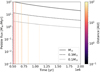 |
Fig. 1 Resulting pebble fluxes from Eq. (16) for Z0 = 0.01 around a solar mass star (solid), a 0.3 M⊕ star (dashed), and a 0.1 M⊕ star (dotted) along with the t0 as described by Eq. (29) for filaments at different separations from the star. |
2.4 Initial conditions and disc model
In this paper, we follow the growth after a localised formation of planetesimals, as has been investigated in multiple previous works (e.g. Lorek & Johansen 2022; Liu et al. 2019b). We did not simulate the concentration of the dust and subsequent collapse to form the initial ring of planetesimals, and we assumed that all the planetesimals are formed at time t0 in our simulation. However, to account for the fact that these processes have to take place before the start of our simulation, we chose the remaining initial conditions to reflect this, which we discuss in further detail in Sect. 2.7. We note that this means we have a different t0 for the different locations in the disc.
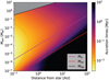 |
Fig. 2 Accretion timescale (Mpl/Ṁpl [Myr]) for a fixed pebble flux and τpeb = 0.1 as a function of the embryo mass Mem and distance from the star with the different transition regimes. |
2.5 Gas disc
To describe the initial gas disc and its evolution, we followed the viscously evolving α disc (Lynden-Bell & Pringle 1974) using the self-similar solution. The temperature profile of the disc was chosen to be (Ida et al. 2016)
 (20)
(20)
We chose a constant α = 10−2 throughout the disc. This resulted in a power-law dependence of the viscosity of  . The evolution of the surface density for our chosen temperature profile and v ~ rγ (γ = 15/14) can be described by the self-similar solution, which is given by
![Mathematical equation: ${\Sigma _} = {{{{\dot M}_{acc,0}}} \over {3\pi v\left( {{r_1}} \right)}}{\left( {r/{r_1}} \right)^{ - \gamma }}{\tau ^{ - (5/2 - \gamma )/(2 - \gamma )}}\exp \left[ { - {1 \over \tau }{{\left( {{r \over {{r_1}}}} \right)}^{2 - \gamma }}} \right].$](/articles/aa/full_html/2025/04/aa52428-24/aa52428-24-eq43.png) (21)
(21)
The characteristic evolution timescale is given by  , and r1 is the characteristic radius (Armitage & Kley 2019). The initial mass accretion rate was chosen to be M⋆,0 = 10−7 M⊙/yr at 0.5 Myr. The total disc mass was set to be Mgas = 0.1 M⋆ at time t = 0, which let us calculate the characteristic radius r1 by integrating the surface density profile (from 0.1 AU to infinity), and we chose r1 so that the total gas mass matches the chosen value. This yielded a characteristic radius of ~72 AU for a solar mass star.
To model the formation around stars with different masses, we had to adapt the disc model and initial conditions. As lower mass stars show lower accretion rates, we scaled the gas disc model with the stellar mass according to Hartmann et al. (2016) linearly Ṁ ∝ M⋆. We kept the disc to stellar mass ratio constant for all stellar masses. This means the characteristic radius r1 is different for different stellar masses. We scaled the luminosity as  , which is consistent with the scaling derived for young stars < 10 Myr that show a range of one to two for the exponent in the L⋆−M⋆ relation for these young stars (Liu et al. 2020).
2.6 Filament
The localised ring of planetesimals modelled in this work was assumed to have formed by streaming instability (Liu et al. 2019b; Gerbig et al. 2020). The typical width of a dense filament of pebbles and the resulting planetesimals forming in them is typically determined by the pressure gradient of the disc  and the separation from the star r0 as ∆w = η ⋅ r0. By postulating a solid-to-gas ratio in the filament Z and a planetesimal formation efficiency factor peff, we could calculate the total mass of planetesimals created in such a filament. The total mass of planetesimals is given by Mfil = 2πr0∆w∑gasZpeff. The IMF of the planetesimals created in these filaments can be described by the cumulative number distribution given by (Schäfer et al. 2017)
![Mathematical equation: ${{{N_ \ge }(m)} \over {{N_{tot{\rm{ }}}}}} = {\left( {{m \over {{m_{min}}}}} \right)^{ - p}}\exp \left[ {{{\left( {{{{m_{min}}} \over {{m_p}}}} \right)}^q} - {{\left( {{m \over {{m_p}}}} \right)}^q}} \right],$](/articles/aa/full_html/2025/04/aa52428-24/aa52428-24-eq47.png) (22)
(22)
where the characteristic planetesimal mass mp is given by
 (23)
(23)
and  is a self-gravity parameter of the gas (Liu & Ji 2020). For the parameters chosen (q = 0.4 and p = 0.6), the mass budget of the planetesimals is dominated by bodies of the characteristic mass mp , whereas the number of bodies is dominated by the smallest bodies Ntot = Mfil/mmin, which was chosen to be mmin = 10−3 mp in our setup (Lorek & Johansen 2022). This allowed us to calculate the largest single body generated in such a filament, which is given by N≥(Mem) = 1. We used this body as the planetary embryo, that is, the initial seed for our forming planet’s core, and we placed it at r0 to track its subsequent growth. As the IMF is strongly peaked around its characteristic mass mp, we initialised the planetesimals as a single-sized population of planetesimals of size
  . The initial surface density of the planetesimals given by
 (24)
(24)
The initial eccentricities and inclinations of the planetesimals are given by e = 2i = η/2 (Lorek & Johansen 2022). Although they are not well constrained from the formation, we know that they have to be smaller than the width of the filament. To visualise the mass scales of the different components described above, we plot the characteristic mass of the planetesimal along with the initial embryo mass and the mass of the entire ring in Fig. 3 for the different stellar masses for our nominal choice of filament metallicity of Z = 0.1.
The initial masses of the planetesimals, the embryo, and the ring increase monotonically with increasing semi-major axis and are lower for lower stellar masses. The ratio of the largest body to the characteristic planetesimal mass stays roughly constant throughout the disc with a ratio of ≈330. We note that the initial mass of the embryo is significantly lower than the initial embryo mass used in most planet formation models (typically 0·01 M⊕).
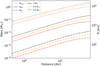 |
Fig. 3 Total ring mass (dotted) and the mass of the single largest (dashed) and characteristic (dashdotted) planetesimal mass for different stellar masses (colour) for filaments with different separations from the star. |
2.7 Initial time
As we assumed the planetesimals to be formed at the start of our simulations, we had to account for the time it took for the dust to grow into pebble sizes and the time required for the pebbles to collapse into planetesimals. We assumed the dust growth to commence in a class-II disc with a typical age of tclassII = 0.5 Myr (Williams & Cieza 2011). To estimate the growth timescale, we followed the approach of Lorek & Johansen (2022). The growth timescale of the dust (Birnstiel et al. 2012) can be described by
 (25)
(25)
where the sticking efficiency given by єp = 0.5 and the Z0 is the dust to gas ratio in the disc. Then, the time required for the dust of initial size r0 to grow to rmax is simply
 (26)
(26)
The growth of the pebbles is limited by two processes: drift and fragmentation. The upper size limit of the pebbles in terms of their Stokes number is described by (Birnstiel et al. 2012)
 (27)
(27)
where vfrag is the fragmentation velocity that we consider to be 1 m/s in this work. The physical size of the pebbles can then be calculated from their Stokes number and assuming Epstein drag via
 (28)
(28)
The time that it takes for the pebbles to collapse into the final planetesimals is on the order of tens to several thousand orbital periods (Yang et al. 2017; Li et al. 2019). Therefore, we used tSI = 500 * 2π/ΩK. This means the initial time of our simulations is considered to be
 (29)
(29)
For our nominal setup around a solar-type star, this results in a time offset from 0.5 Myr in the inner disc up to ~1 Myr at 100 AU. The results shown in the following section all display the time relative to the initial time t0 of the simulation.
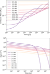 |
Fig. 4 Embryo masses for filaments at different separations from the star over time (top) and the surface density of planetesimals in the ring (bottom) as a function of time. |
3 Results
We probed the formation of embryos in filaments at different locations ranging from 0.5 to 50 AU from their initial time t0 to 10 Myr, which serves as a reasonable upper bound for the gas disc lifetime. The growth of the embryos and the evolution of the surface density of the planetesimals at the different separations from the star for our nominal model can be seen in Fig. 4. The parameters of our nominal setup are a metallicity of Z = 0.1 for the filament with a Mgas = 0.1 M⊙ gas disc around a solar mass star, and we did not include pebble accretion and fragmentation. The remaining parameters of the nominal simulation can be found in Table B.1.
As dictated by our initial conditions, the initial mass of the embryos ascends with increasing separation from the star (see Fig. 3). However, due to the higher surface density of planetesimals and the higher orbital frequency closer to the star, the embryos closer in can grow significantly faster and accrete all the mass in their filament, whereas with increasing distance, the growth of the largest body is significantly slower, making it almost negligible at 50 AU. The surface density of the planetesimals in the ring starts to decrease even at early times due to the diffusion of the planetesimals, which is caused by their mutual gravitational interaction and acts as a further barrier to the growth of the embryo, as it directly relates to the accretion rate that is shown in the bottom panel of Fig. 4. To get a better idea of how the filaments at different separations evolve in time, we plot the embryo masses throughout time for the filaments at the different semi-major axes in Fig. 5. We also include a plot of the characteristic mass of the planetesimals and the total mass contained in the filament. To better visualise where pebbles could be accreted efficiently (although pebble accretion is not considered for this set of simulations), we plotted the different efficiency regimes according to the transitions from ballistic to Bondi and Bondi to Hill, respectively, as described in Sect. 2.3. As one can see, the initial mass of the largest body (i.e. the embryo) is quite close to the transition mass (by a factor of ≈1.5) for the filaments up to 10 AU. Even so, the growth of the largest body from planetesimal accretion is only significant enough to reach the transition mass up to ~10 AU. Farther out, there is virtually no growth, and the embryo fails to accrete any significant amount of mass from the planetesimal ring. However, in the inner disc, the embryo is able to accrete the entire mass of the filament up to ~2 AU. Whereas, in the intermediate regime, the growth is too slow to accrete all the material. This growth pattern is consistent with previous studies (Lorek & Johansen 2022), which also show this stark radial dependence of embryo growth.
To investigate the impact different physical processes have on the early growth in these filaments, we first ran simulations with the same setup as above, but we included additional physical effects, for example, fragmentation and the effect diffusion has on early growth. Additionally, we investigated the formation around lower-mass stars when considering planetesimal accretion only. Then, we investigated how the early growth is impacted when we consider the accretion of pebbles concurrently. Finally, we discuss the implications of our results for the timing of core formation and how it can inform the initial conditions of global formation models.
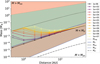 |
Fig. 5 Mass of the largest body in the ring (embryo; solid), the initial characteristic planetesimal mass (dash doted), and ring mass (dotted). The background colours refer to the different pebble accretion regimes (red: ballistic/isolation regime; brown: Bondi regime; and green: Hill regime). |
3.1 Fragmentation
As described by Lorek & Johansen (2022), the consideration of fragmentation can have an effect on the mass growth and final mass of the embryo forming in these rings. To investigate this, we also ran a set of simulations that include the effect of frag mentation with the collision model as described in Sect. 2.2. illustrate the effect fragmentation has on the growth of embry in Fig. 6 we show the surface densities of initial planetesim and the fragments, that is, the sum over all the planetesimal mass bins smaller than the initial planetesimal mass that get created via collisions in the ring in Fig. 6.
As one can clearly see, the number of fragments and the speed at which they are created is significantly shorter in the inner disc, whereas virtually no fragments are created in the outer disc. This can be explained by the longer collision timescales caused by the lower surface densities, scaling with separation, and a bigger initial planetesimal size leading to a higher specific material strength of the initial planetesimals (Benz & Asphaug 1999). The resulting growth of the filaments including fragmentation can be seen in Fig. 7. The final mass of the largest body within 1 AU is smaller than its non-fragmenting counterpart due to the fact that some of the mass excavated the collisions is deposited into dust (i.e. mass deposited in sizes below rmin), which is considered to be lost in our model for the purposes of accretion. However, the growth of the filament at intermediate separations between ~1–5 AU is enhanced when the embryo approaches the filament mass, as the embryo starts to stir up the relative velocities of the planetesimals. This leads to higher final masses for the bodies, as the fragments are easier to accrete because they are more tightly bound to the gas. As indicated by the number of fragments produced and the growth track, fragmentation plays virtually no role in the growth of the embryo in the outer disc, which is in line with previous findings (Kaufmann & Alibert 2023; Lorek & Johansen 2022). We note that due to computational constraints, we evolved the simulations only for 6 Myr.
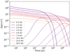 |
Fig. 6 Surface density of the planetesimals (solid) and fragments (dashed) for the filaments at different separations. |
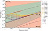 |
Fig. 7 Same as Fig. 5 but with the addition of the mass lost from collisions among planetesimals (dark red). |
3.2 Effect of diffusion
The diffusive widening of the ring of planetesimals reduces their surface density, as can be seen in Fig. 4, which slows down the growth of the embryo. To understand the importance of this effect, we performed a set of simulations where we set the diffusion term in Eq. (3) to zero. Although nonphysical, it illustrates a setup closer to the formation in structured discs that act as migration traps due to a change in the gas pressure gradient (Jiang & Ormel 2022). The growth of the different filaments without diffusion can be seen in Fig. 8.
The growth of the embryos is significantly enhanced when diffusion is not considered since it allows the largest body to accrete the entire mass contained in the filament up to ~7 AU. Additionally, it also allows the largest body to grow to the transition mass for a larger separation up to 25 AU. This clearly demonstrates a difference in growth patterns when we consider a radially localised distribution of planetesimals.
3.3 Varying stellar mass
As planet formation strongly depends on the mass of its host star, we additionally ran a set of simulations for a host star with a mass of 0.3 and a 0.1 M⊙. The changes in the disc model and the initial conditions are outlined in Sect. 2.5, and the change in mass for the ring and planetesimals can be seen in Fig. 3. We note that in order to keep the disc star mass ratio constant (i.e. Mgas = 0.1 M⋆), the characteristic radius of the gas disc varies for different stellar masses. In Fig. 9, we show the growth of the filaments for a 0.3 M⊕ (top) and a 0.1 M⊙ (bottom) mass star at different separations, using the nominal setup, in Fig. 9.
As can be clearly seen in the figure, the growth around both the 0.3 and 0.1 M⊙ mass stars are significantly reduced. For the 0.3 M⊙ star, the filaments up to 3 AU are able to reach the transition mass, whereas for the 0.1 M⊙ star, this only happens up to ~1 AU. This can easily be explained as being due to how the chosen initial conditions and the characteristic masses scale with the mass of the host star. That is, the embryos need to grow significantly more in order to reach the transition mass Mtr for lower stellar masses. Although the ring properties are dependent on the distance from the star, the following scaling relations we derived are valid for planetesimal rings with separations of up to 10 AU from the star. We outline how the different components scale with the mass of the host star in order to explain the aforementioned differences in early growth of the embryo for a varying stellar mass. Farther out, there is a radial dependence of these scaling laws due to the different characteristic radii and growth times (leading to different t0), so the following relations are only applicable to the inner disc, where the initial gas surface density scales as  (which was fitted to the initial disc profiles around different stellar masses). As a result of the chosen initial conditions, the characteristic planetesimal mass given in Eq. ( scales as
  with the stellar mass of the host star. This leads to a scaling of the mass of the largest body according to
  . We note that these relations are not derived fully analytically, as the initial planetesimal surface density and embryo mass were calculated from implicit equations. For chosen disc model, the transition mass scales as
  The onset mass for pebble accretion scales either as
  or
or  , depending on whether we choose to consider the Stokes number for the pebbles to be fixed or if it is given by the fragmentation size limit in Eq. (27). This makes it quite apparent that the formation of massive embryos around higher- mass stars is a lot easier, as the initial masses of the embryos are greater, and transitions of the pebble accretion regimes hap at lower masses. This illustrates well that the largest planetesimals are smaller around lower-mass stars and the characteristic masses of pebble accretion are larger, making it harder to form massive embryos around these stars.
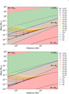 |
Fig. 9 Same as Fig. 5 but for filaments around a 0.3 M⊙ mass star (top) and around a 0.1 M⊙ mass star (bottom). |
3.4 Including pebble accretion
Thus far we have ignored the fact that although the accretion of pebbles is in the less efficient Bondi regime for initial masses of bodies created by streaming instability, it still contributes to the mass growth of the larger bodies. Therefore, we modelled the accretion of pebbles onto the embryo using the approach outlined in Liu et al. (2019b), considering a radially constant flux of pebbles with a fixed Stokes number of τs = 0.1. We calculated the pebble flux using the approach of Lambrechts & Johansen (2014). The resulting pebble flux along with the initial time t0 of the different rings due to their different growth timescales and the times it takes for the planetesimals to collapse can be seen in Fig. 1. We ignored the pebble accretion on the smaller planetesimals, as their masses are significantly lower than the onset mass for all our setups, and therefore pebble accretion is suppressed. The growth of the largest body when pebble accretion is included for the filaments throughout the disc is shown in Fig. 10.
In the figure, one can clearly see that with the addition of pebble accretion, growth is significantly enhanced for filaments at all distances from the star. Up until a few au, this even allows the largest body to reach the isolation mass at which the accretion of pebbles is stopped and the rapid accretion of gas should commence. However, at larger separations beyond 25 AU, it still takes a significant amount of time for the embryo to grow, and due to the decay of the pebble flux, the embryo never reaches the isolation mass. To probe the growth mode in the rings, in Fig. 11 we plot the mass of the embryos throughout time at varying locations along with the mass they accreted from planetesimals (dashed) and pebbles (dotted) and with the time where the pebble accretion changes regimes, that is, from the Bondi to the Hill regime (cross). As expected, the accretion from planetesimals only plays a role in the very beginning and is quickly overtaken by the pebble accretion. We observed that for all separations, the planetesimals are the main growth mode only for very early times and that pebble accretion quickly becomes the dominant source of accretion for the largest body. This clearly shows that even for this early growth phase, the accretion of pebbles cannot be neglected.
To probe the influence the dynamical size of the pebbles has on the early growth, we ran the same set of simulations as mentioned before but considering pebbles of a fixed lower Stokes number of τs = 0.03. We show the results of these simulations in Fig. 12 along with a comparison with the growth tracks considering the accretion of pebbles with different aerodynamic sizes. We observed that, initially, the (aerodynamically) larger pebbles result in higher accretion rates; however, at higher embryo masses, this trend reverses, leading to faster growth from smaller pebbles. In the inner disc, the embryo reaches the isolation mass at earlier times for the smaller pebbles, and in the outer disc, this results in higher final masses. The results show that overall, the early growth is enhanced for pebbles of these lower Stokes numbers for the same pebble flux. To check how consistent the choice of pebbles with a fixed Stokes number is in the drift size limit, we computed the Stokes numbers in the local drift limit following the approach of Izidoro et al. (2021), which yielded Stokes numbers of τs ~ 0.01–0.07. This motivated us to explore this second set of simulations with a fixed lower Stokes number.
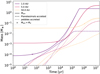 |
Fig. 11 Total mass of the embryo (solid), the mass budget of planetesimals accreted (dashed), and mass of accreted pebbles (dotted). |
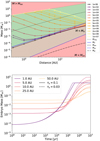 |
Fig. 12 Same as Fig. 10 but for pebbles with a Stokes number of τs = 0.03 (top); mass of the embryo (bottom) considering the accretion of pebbles with τs = 0.1 (solid) and τs = 0.03 (dashed). |
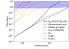 |
Fig. 13 Time required for the embryo to reach the transition mass for the nominal simulations without pebble accretion (solid) when considering the time-dependent pebble flux (dashed) and the fixed pebble flux (dotted) for different stellar masses (colour). The blue-shaded region refers to the time after which the gas surface density is reduced by half. |
3.5 The timing of core formation
As many global planet formation models start with partially assembled cores as their initial conditions (Emsenhuber et al. 2021; Liu et al. 2019a; Savvidou & Bitsch 2025; Venturini et al. 2020, 2024), it is important to constrain the timing of when bodies of that size are able to form. Therefore, an interesting metric to investigate is the time at which a filament can produce the seed for efficient pebble accretion is the time that the largest body reaches the transition mass described in Eq. (18), or if an embryo of that mass can even form out of planetesimal rings. Thus, we calculated the transition time Mem (ttr) = Mtr, that is, the time it takes for the single largest planetesimal to grow to the transition mass for our different aforementioned setups, including the simulations considering pebble accretion and those without it. In addition to the simulations with a time-dependent pebble flux, we also performed a set of simulations but considered a pebble flux that is fixed in the time of Fpeb = 50 M⊕/Myr for reference.
In Fig. 13, we plot the time in the simulation at which the largest body reaches Mtr as described in Eq. (18) to better understand the timing of embryo formation for the simulations only considering planetesimal accretion, the time-dependent pebble flux, and the constant pebble flux and for the different stellar masses. We also highlight the time at which the gas surface density has reduced by half of the initial value as a proxy for the disc lifetime, as we did not consider external photoevaporation or other mass-loss mechanisms for our gas disc. As can be clearly seen, the time needed to reach the transition mass monotonically increases with distance from the star and with decreasing stellar mass. One can also see that the addition of pebble accretion reduces the time to reach the transition significantly, although the effect is more visible for the rings at larger separations, as in the inner disc there is still a significant contribution from planetesimal accretion.
Additionally, to probe the influence of the IMF of the planetesimals and the properties of the initial filament, we performed another set of simulations considering a reduced filament metallicity of Z = 0.01 and one where we reduced the initial mass of the largest planetesimal by a factor of ten while keeping the total mass constant. The results of this investigation can be seen in Fig. 14, where we once again plot the time for the largest planetesimal to reach the transition mass.
As we expected, the reduction in initial embryo mass leads to a significantly longer formation timescale so that outside of a few AU, the embryo is not able to reach the transition mass at all. The simulations with reduced metallicity showed a very similar picture but with even slightly longer timescales, as in addition to a reduced initial embryo mass, the surface density of the planetesimals is also reduced, leading to longer accretion timescales.
To gain an idea of which model parameters influence the timing of embryo formation the most and offer a simple description that can inform population synthesis models as to what time to insert the initial partially assembled embryos in their simulations, we performed a grid of simulations where we varied multiple key model parameters: the semi-major axis of the filament, the stellar mass, the pebble flux, and the mass of the largest embryo. The timing of embryo formation was inferred by calculating the transition timing for each simulation. In Table 1, we present the grid chosen for the different parameters along with the nominal value. We note that we varied the initial embryo mass as a factor of the nominal model (i.e. Mem,grid = fem * Mem,0) rather than choosing a fixed value in order to keep the investigated scenario consistent with the planetesimal IMF we considered. A visualisation of the simulation results can be seen in Fig. 15, where for a fixed stellar mass, we plot the transition timing for the remaining parameter pairs. In the interest of brevity, the same plots for further stellar masses can be found in Fig. C.1. Additionally, in Fig. 16, we plot the transition timing for different stellar masses at different distances to show the influence of the stellar mass on core formation.
As expected, we recovered the observed behaviour of the effects of the distance from the star and the pebble flux on the transition timing. We also observed that the effect of the distance is much more important for the formation time when compared to the pebble flux whose influence is lower, especially for the solar mass star and in the inner disc. The initial embryo mass is highly important for the subsequent growth, and its effect dominates over the pebble flux but is less influential around lower-mass stars (as can be seen in Fig. C.1), where the pebble flux gains more importance. This is consistent with the simulations with a higher metallicity that we ran for low-mass stars that did not enhance growth significantly. To make the data easily accessible, they have been uploaded as a Python package to GitHub,1 which contains the transit timings for all the simulations along with the time (if) the embryo reaches 10–3 and 10–2 M⊕. We note that even though the calculated initial times are model dependent and therefore should be treated as an estimate, due to the modular nature of the model, it can be easily adapted to various scenarios by, for example, changing the disc and planetesimal IMF, which we aim to explore in future works.
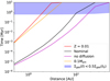 |
Fig. 14 Same as Fig. 13 but for the following setups: nominal (black), with a reduced initial embryo mass (yellow), reduced filament metallicity (red), and ignoring diffusion (magenta). |
Parameter grid for the simulations to infer the timing of embryo formation.
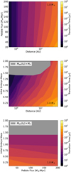 |
Fig. 15 Transition timing (colour) for the grid simulations around a 1 M⊙ mass star as a function of two grid dimensions, where the last variable not plotted is given by the bold value in Table 1. The grey area refers to simulations where the initial embryo is already larger than the transition mass. |
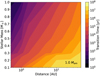 |
Fig. 16 Transition timing of the grid at different stellar masses and separations where Fpeb = 100 M⊕/Myr and Mem = 1 Mem,0. |
4 Discussion and conclusions
4.1 Limitations of the model
There are several simplifications that we made for the model described in this paper that have to be discussed. Firstly, we neglected the migration of both the embryo and the planetesimals. However, in the mass regime of the embryo, we state in this paper that the migration timescales are much longer than the time it takes to reach the transition masses; nevertheless, for the cases where the embryo grows larger, up to its isolation mass, these effects should be considered (Paardekooper et al. 2011; Ida et al. 2020). Due to the fact that the torque generated by the disc onto the planet scales with the planet’s mass until the embryos reach the transition mass, planet migration should not play a relevant role (Tanaka et al. 2002; Paardekooper et al. 2011; Ida et al. 2020). However, when the mass of the embryo exceeds the transition mass, planet migration could be too crucial to be ignored. In addition, if pebble accretion becomes very efficient, thermal torques (Guilera et al. 2021; Baumann & Bitsch 2020) or dust torques (Guilera et al. 2023) could be relevant as well.
Regarding the planetesimals, for those of initial sizes rp > 10 km, the drift is negligible (Ormel & Kobayashi 2012), and only for planetesimals of radii ≲1 km does planetesimal drift play an important role (Guilera et al. 2010; Guilera & Sándor 2017). For the fragments produced in collisions, the radial transport is significant, as it leads to further depletion of solids in the ring, so our simulations can be seen as upper limits when we include the fragmentation of planetesimals. The choice of the IMF of the planetesimals significantly shapes the nature of the subsequent growth in the ring (Liu et al. 2019b). However, as planetesimal formation is a very active field of research, the precise nature of the IMF remains very uncertain both from a formation point (Polak & Klahr 2022; Schäfer et al. 2017) and also from observational constraints (Morbidelli et al. 2009; Schlichting et al. 2013) from the Solar System. Therefore, we limited ourselves to the IMF as described in Sect. 2.5. Additionally, our model only considers the formation in a single ring, whereas a fully global model could model the formation of many concurrently forming planets and rings, leading to interactions between them, for example, by reducing the pebble flux for further filaments downstream.
For this study, we chose simple dust evolution and pebble accretion models, as they made it easier to investigate the influence of the different model parameters (e.g. the pebble flux or Stokes number) on the early growth stage. However, as a tradeoff, there are certain characteristics of pebble accretion we had to neglect. Firstly, even though we inferred the pebble flux from the disc properties (Lambrechts & Johansen 2014), we did not calculate the dust and pebble properties self-consistently throughout the disc as could be done by modelling the dust evolution using models of varying complexity (e.g. Drazkowska et al. 2021; Pfeil et al. 2024; Stammler & Birnstiel 2022). This would then also allow us to account for the shift in accretion efficiencies due to the presence of pebbles of different sizes. Lyra et al. (2023) have shown that accounting for the size distribution of pebbles significantly changes the accretion efficiency in the Bondi regime. This would promote enhanced early growth; that is, it would reduce the effective onset mass of pebble accretion. Using their description of poly-disperse pebble accretion, the works of Lyra et al. (2023) shows that the initial embryos in the same mass range as considered in this work show significantly lower accretion timescales compared to single-size pebbles. The higher accretion rates due to the presence of pebbles of smaller sizes were qualitatively shown in Fig. 12, but properly accounting for the poly-disperse nature of the pebble flux is beyond the scope of this work (and incompatible with the analytic calculation of the pebble flux), and it will therefore be explored in future works.
4.2 Conclusions and summary
In this paper, we have investigated the early growth of a planetary embryo from a ring of planetesimals to sizes large enough to accrete pebbles efficiently. We developed a formation model that tracks the evolution of a ring of planetesimals created from streaming instability. We simulated the planetesimals and the largest body, including the relevant physics to evolve the system self-consistently considering the evolution of the random velocities’ mutual collisions and pebble accretion. Our main findings are as follows:
Growing the seed of pebble accretion from a planetesimal ring when only considering the growth from planetesimal accretion is possible only in the inner disc (< 1 AU) and on short timescales. However, the embryo growth from planetesimal accretion is negligible at large separations;
The diffusion of the planetesimal ring is a major inhibitor for the growth of the largest body;
The inclusion of pebble accretion cannot be neglected, as it contributes significantly to the growth of the embryo, even in the slower Bondi regime. Still, at a large separation of ≈50 AU, it takes a considerable amount of time for the largest planetesimal to reach the transition mass from the Bondi to the Hill regime;
For lower stellar masses, the growth of the largest body is slower, and even at moderate distances of ≈1–10 AU, it remains hard to grow the core of planets within the typical lifetime of protoplanetary discs. These results could be related to the lack of giant planets compared to more massive stars (Sabotta et al. 2021);
The timing of core formation is strongly dependent on stellar mass and semi-major axis, which should be taken into account for formation models starting with partially assembled cores.
Understanding the formation pathway presented in this work and in similar works (Liu et al. 2019b; Jiang & Ormel 2022; Lorek & Johansen 2022) is vital to constraining the early stages of planet formation and the interplay of planetesimal formation and planetesimal and pebble accretion. However, these works all consider the isolated formation of planets at a single location. This calls for the investigation of these formation scenarios using global evolution models that allow for the formation of planetesimals in multiple rings and interaction among them (Lau et al. 2024). Furthermore, it highlights the necessity to better constrain the IMF of planetesimals, as it has a major impact on the subsequent growth in these filaments.
Acknowledgements
O.M.G. gratefully acknowledges the invitation and financial support from the International Space Science Institute (ISSI) Bern in early 2024. This research was partially supported through the Visiting Scientist program of the ISSI in Bern. O.M.G. and I.L.S.S. are partially supported by PIP-2971 from CONICET (Argentina) and by PICT 2020-03316 from Agencia I+D+i (Argentina). We acknowledge the support from the NCCR PlanetS.
Appendix A Validation and comparison of the fragmentation model
 |
Fig. A.1 Growth track of a moon-mass embryo at 5 AU in our model (blue) and (Guilera et al. 2014) with only the local collisions (red) and the multi-annulus case (green). |
To test the validity of the simplifications made in the fragmentation model derived in this work we compare it against the model implemented in Guilera et al. (2014) and Sebastián et al. (2019). To do this, and to isolate the effects of the fragmentation description the treatment of the remaining physics is kept as simple as possible to perform the comparison. We computed the formation of a planet just considering the accretion of planetesimals of 100 km radius and the fragments generated by the planetesimal fragmentation process; that is, we did not consider gas accretion onto the planet or the enhancement in the planet’s cross-section of the capture radius due to the presence of an envelope. We consider the same initial conditions as in Guilera et al. (2014) and Sebastián et al. (2019), that is the growth of an initial mass Moon embryo located at 5 AU and immersed in a planetesimal disc ten times more massive than the minimum mass solar nebula (Hayashi 1981). The gas disc is considered to decay with a characteristic timescale of 6 Myr. Additionally, we do not consider accreting collisions among planetesimals meaning collisions where Equation 4 MR > MT in Eq. (4). We note that we only consider the fragmentation of planetesimals that belong to the same annulus (as in Kaufmann & Alibert 2023), but for the sake of comparison we also compute the multi-annulus case, that is where targets and projectiles can belong to different annulus. In figure A.1 we can see the resulting growth track of the planetary embryo using the different codes.
The growth tracks in both models are a good match. Our code seems to have slightly faster growth leading to an increased final mass which can be explained because of the way we calculate the feeding zone which differs in both codes (Guilera et al. (2014) considers a feeding zone with a half-width of 4Rh with a soothing function whereas we consider at top with a half-width of 5Rh) as this difference shows up before the first fragments are created. As the focus of this comparison is the fragmentation model we are also interested in the size distribution of the planetesimals at the planet’s location throughout the formation process. To illustrate those we show in Fig. A.2 the surface density distribution of the different sizes at 4 Myr in both models.
As we can see even though there are some differences in the size distribution they seem to fit very well overall however for the smaller sizes there seem to be some deviations stemming from the fact that we only consider local collisions and that for a given time the embryo in both simulations does not have the same mass resulting in a slight difference in the evolution of the size distribution of the planetesimals.
 |
Fig. A.2 Surface density distribution of the planetesimals at the location of the planet calculated using our model (blue) and the model presented in Guilera et al. (2014) with only the local collisions (red) and the multi-annulus case (green). |
Appendix B Model parameters
Table with the chosen parameters for the simulations.
Appendix C Grid simulations
References
- Abod, C. P., Simon, J. B., Li, R., et al. 2019, ApJ, 883, 192 [Google Scholar]
- Armitage, P. J., & Kley, W. 2019, Saas-Fee Advanced Course, 45, eds. M. Audard, M. R. Meyer, & Y. Alibert (Berlin, Heidelberg: Springer Berlin Heidelberg) [Google Scholar]
- Ataiee, S., Baruteau, C., Alibert, Y., & Benz, W. 2018, A&A, 615, A110 [NASA ADS] [CrossRef] [EDP Sciences] [Google Scholar]
- Bai, X.-N., & Stone, J. M. 2010, ApJ, 722, 1437 [NASA ADS] [CrossRef] [Google Scholar]
- Baumann, T., & Bitsch, B. 2020, A&A, 637, A11 [NASA ADS] [CrossRef] [EDP Sciences] [Google Scholar]
- Benz, W., & Asphaug, E. 1999, Icarus, 142, 5 [NASA ADS] [CrossRef] [Google Scholar]
- Bae, J., Isella, A., Zhu, Z., et al. 2023, arXiv e-prints [arXiv:2210.13314] [Google Scholar]
- Benz, W. 2000, in From Dust to Terrestrial Planets, 9, eds. W. Benz, R. Kallenbach, & G. W. Lugmair (Dordrecht: Springer Netherlands), 279 [NASA ADS] [CrossRef] [Google Scholar]
- Birnstiel, T. 2023, arXiv e-prints [arXiv:2312.13287] [Google Scholar]
- Birnstiel, T., Ormel, C. W., & Dullemond, C. P. 2011, A&A, 525, A11 [NASA ADS] [CrossRef] [EDP Sciences] [Google Scholar]
- Birnstiel, T., Klahr, H., & Ercolano, B. 2012, A&A, 539, A148 [NASA ADS] [CrossRef] [EDP Sciences] [Google Scholar]
- Bitsch, B., Morbidelli, A., Johansen, A., et al. 2018, A&A, 612, A30 [NASA ADS] [CrossRef] [EDP Sciences] [Google Scholar]
- Carrera, D., Gorti, U., Johansen, A., & Davies, M. B. 2017, ApJ, 839, 16 [Google Scholar]
- Chambers, J. E. 2006a, ApJ, 652, L133 [NASA ADS] [Google Scholar]
- Chambers, J. 2006b, Icarus, 180, 496 [NASA ADS] [CrossRef] [Google Scholar]
- Chatterjee, S., & Tan, J. C. 2013, ApJ, 780, 53 [NASA ADS] [CrossRef] [Google Scholar]
- Drążkowska, J., & Alibert, Y. 2017, A&A, 608, A92 [Google Scholar]
- Drazkowska, J., Stammler, S. M., & Birnstiel, T. 2021, A&A, 647, A15 [EDP Sciences] [Google Scholar]
- Emsenhuber, A., Mordasini, C., Burn, R., et al. 2021, A&A, 656, A69 [NASA ADS] [CrossRef] [EDP Sciences] [Google Scholar]
- Gerbig, K., Murray-Clay, R. A., Klahr, H., & Baehr, H. 2020, ApJ, 895, 91 [CrossRef] [Google Scholar]
- Guilera, O. M., & Sándor, Z. 2017, A&A, 604, A10 [Google Scholar]
- Guilera, O. M., Brunini, A., & Benvenuto, O. G. 2010, A&A, 521, A50 [NASA ADS] [CrossRef] [EDP Sciences] [Google Scholar]
- Guilera, O. M., de Elía, G. C., Brunini, A., & Santamaría, P. J. 2014, A&A, 565, A96 [NASA ADS] [CrossRef] [EDP Sciences] [Google Scholar]
- Guilera, O. M., Sándor, Z., Ronco, M. P., Venturini, J., & Bertolami, M. M. M. 2020, A&A, 642, A140 [NASA ADS] [CrossRef] [EDP Sciences] [Google Scholar]
- Guilera, O. M., Bertolami, M. M. M., Masset, F., et al. 2021, MNRAS, 507, 3638 [NASA ADS] [CrossRef] [Google Scholar]
- Guilera, O. M., Benitez-Llambay, P., Miller Bertolami, M. M., & Pessah, M. E. 2023, ApJ, 953, 97 [NASA ADS] [CrossRef] [Google Scholar]
- Güttler, C., Blum, J., Zsom, A., Ormel, C. W., & Dullemond, C. P. 2010, A&A, 513, A56 [Google Scholar]
- Hartmann, L., Herczeg, G., & Calvet, N. 2016, Annu. Rev. Astron. Astrophys., 54, 135 [Google Scholar]
- Hayashi, C. 1981, Progr. Theor. Phys. Suppl., 70, 35 [Google Scholar]
- Hu, X., Tan, J. C., Zhu, Z., et al. 2018, ApJ, 857, 20 [NASA ADS] [CrossRef] [Google Scholar]
- Ida, S., Guillot, T., & Morbidelli, A. 2016, A&A, 591, A72 [NASA ADS] [CrossRef] [EDP Sciences] [Google Scholar]
- Ida, S., Muto, T., Matsumura, S., & Brasser, R. 2020, MNRAS, 494, 5666 [Google Scholar]
- Inaba, S. 2001, Icarus, 149, 235 [CrossRef] [Google Scholar]
- Izidoro, A., Bitsch, B., Raymond, S. N., et al. 2021, A&A, 650, A152 [EDP Sciences] [Google Scholar]
- Jang, H., Liu, B., & Johansen, A. 2022, A&A, 664, A86 [NASA ADS] [CrossRef] [EDP Sciences] [Google Scholar]
- Jiang, H., & Ormel, C. W. 2021, MNRAS, 505, 1162 [NASA ADS] [CrossRef] [Google Scholar]
- Jiang, H., & Ormel, C. W. 2022, MNRAS, 518, 3877 [NASA ADS] [CrossRef] [Google Scholar]
- Johansen, A., & Youdin, A. 2007, ApJ, 662, 627 [Google Scholar]
- Johansen, A., Oishi, J. S., Mac Low, M.-M., et al. 2007, Nature, 448, 1022 [Google Scholar]
- Johansen, A., Youdin, A., & Klahr, H. 2009, ApJ, 697, 1269 [Google Scholar]
- Kaufmann, N., & Alibert, Y. 2023, A&A, 676, A46 [NASA ADS] [CrossRef] [EDP Sciences] [Google Scholar]
- Klahr, H., & Schreiber, A. 2020, ApJ, 901, 54 [NASA ADS] [CrossRef] [Google Scholar]
- Kobayashi, H., & Tanaka, H. 2018, ApJ, 862, 127 [Google Scholar]
- Krijt, S., Ormel, C. W., Dominik, C., & Tielens, A. G. G. M. 2015, A&A, 574, A83 [NASA ADS] [CrossRef] [EDP Sciences] [Google Scholar]
- Krivov, A. V., Ide, A., Löhne, T., Johansen, A., & Blum, J. 2018, MNRAS, 474, 2564 [NASA ADS] [CrossRef] [Google Scholar]
- Lambrechts, M., & Johansen, A. 2014, A&A, 572, A107 [NASA ADS] [CrossRef] [EDP Sciences] [Google Scholar]
- Lau, T. C. H., Drążkowska, J., Stammler, S. M., Birnstiel, T., & Dullemond, C. P. 2022, A&A, 668, A170 [NASA ADS] [CrossRef] [EDP Sciences] [Google Scholar]
- Lau, T. C. H., Birnstiel, T., Drążkowska, J., & Stammler, S. 2024, A&A, 688, A22 [NASA ADS] [CrossRef] [EDP Sciences] [Google Scholar]
- Lau, T. C. H., Lee, M. H., Brasser, R., & Matsumura, S. 2024, A&A, 683, A204 [NASA ADS] [CrossRef] [EDP Sciences] [Google Scholar]
- Leinhardt, Z. M., & Stewart, S. T. 2012, arXiv e-prints [arXiv:1106.6084] [Google Scholar]
- Lenz, C. T., Klahr, H., & Birnstiel, T. 2019, ApJ, 874, 36 [NASA ADS] [CrossRef] [Google Scholar]
- Li, R., Youdin, A. N., & Simon, J. B. 2019, ApJ, 885, 69 [NASA ADS] [CrossRef] [Google Scholar]
- Liu, B., & Ji, J. 2020, Res. Astron. Astrophys., 20, 164 [Google Scholar]
- Liu, B., & Ormel, C. W. 2018, A&A, 615, A138 [NASA ADS] [CrossRef] [EDP Sciences] [Google Scholar]
- Liu, B., Lambrechts, M., Johansen, A., & Liu, F. 2019a, A&A, 632, A7 [NASA ADS] [CrossRef] [EDP Sciences] [Google Scholar]
- Liu, B., Ormel, C. W., & Johansen, A. 2019b, A&A, 624, A114 [NASA ADS] [CrossRef] [EDP Sciences] [Google Scholar]
- Liu, B., Lambrechts, M., Johansen, A., Pascucci, I., & Henning, T. 2020, A&A, 638, A88 [EDP Sciences] [Google Scholar]
- Lorek, S., & Johansen, A. 2022, A&A, 666, A108 [NASA ADS] [CrossRef] [EDP Sciences] [Google Scholar]
- Lynden-Bell, D., & Pringle, J. E. 1974, MNRAS, 168, 603 [Google Scholar]
- Lyra, W., Johansen, A., Cañas, M. H., & Yang, C.-C. 2023, arXiv e-prints [arXiv:2301.03825] [Google Scholar]
- Morbidelli, A., Bottke, W., Nesvorny, D., & Levison, H. F. 2009, Icarus, 204, 558 [NASA ADS] [CrossRef] [Google Scholar]
- Ohtsuki, K., & Tanaka, H. 2003, Icarus, 162, 47 [NASA ADS] [CrossRef] [Google Scholar]
- Ohtsuki, K., Stewart, G. R., & Ida, S. 2002, Icarus, 155, 436 [Google Scholar]
- Ormel, C. W. 2017, in Formation, Evolution, and Dynamics of Young Solar Systems, 445, eds. M. Pessah & O. Gressel (Cham: Springer International Publishing), 197 [NASA ADS] [CrossRef] [Google Scholar]
- Ormel, C. W., & Kobayashi, H. 2012, ApJ, 747, 115 [NASA ADS] [CrossRef] [Google Scholar]
- Ormel, C. W., & Liu, B. 2018, A&A, 615, A178 [NASA ADS] [CrossRef] [EDP Sciences] [Google Scholar]
- Paardekooper, S.-J., Baruteau, C., & Kley, W. 2011, MNRAS, 410, 293 [NASA ADS] [CrossRef] [Google Scholar]
- Pfeil, T., Birnstiel, T., & Klahr, H. 2024, A&A, 691, A45 [NASA ADS] [CrossRef] [EDP Sciences] [Google Scholar]
- Pinilla, P., Lenz, C. T., & Stammler, S. M. 2021, A&A, 645, A70 [NASA ADS] [CrossRef] [EDP Sciences] [Google Scholar]
- Pinte, C., Teague, R., Flaherty, K., et al. 2022 [Google Scholar]
- Polak, B., & Klahr, H. 2022, arXiv e-prints [arXiv:2211.13318] [Google Scholar]
- Pollack, J. B., Hubickyj, O., Bodenheimer, P., et al. 1996, Icarus, 124, 62 [NASA ADS] [CrossRef] [Google Scholar]
- Sabotta, S., Schlecker, M., Chaturvedi, P., et al. 2021, A&A, 653, A114 [NASA ADS] [CrossRef] [EDP Sciences] [Google Scholar]
- Sándor, Zs., Guilera, O. M., Regály, Zs., & Lyra, W. 2024, A&A, 686, A78 [NASA ADS] [CrossRef] [EDP Sciences] [Google Scholar]
- Savvidou, S., & Bitsch, B. 2025, A&A, 693, A302 [NASA ADS] [Google Scholar]
- Schäfer, U., Yang, C.-C., & Johansen, A. 2017, A&A, 597, A69 [Google Scholar]
- Schlichting, H. E., Fuentes, C. I., & Trilling, D. E. 2013, AJ, 146, 36 [NASA ADS] [CrossRef] [Google Scholar]
- Schneider, A. D., & Bitsch, B. 2021, A&A, 654, A71 [Google Scholar]
- Schoonenberg, D., & Ormel, C. W. 2017, A&A, 602, A21 [NASA ADS] [CrossRef] [EDP Sciences] [Google Scholar]
- Sebastián, I. L. S., Guilera, O. M., & Parisi, M. G. 2019, A&A, 625, A138 [NASA ADS] [CrossRef] [EDP Sciences] [Google Scholar]
- Shibaike, Y., & Alibert, Y. 2020, A&A, 644, A81 [NASA ADS] [CrossRef] [EDP Sciences] [Google Scholar]
- Shibaike, Y., & Alibert, Y. 2023, A&A, 678, A102 [NASA ADS] [CrossRef] [EDP Sciences] [Google Scholar]
- Stammler, S. M., & Birnstiel, T. 2022, ApJ, 935, 35 [NASA ADS] [CrossRef] [Google Scholar]
- Stammler, S. M., Drażkowska, J., Birnstiel, T., et al. 2019, ApJ, 884, L5 [NASA ADS] [CrossRef] [Google Scholar]
- Stewart, S. T., & Leinhardt, Z. M. 2009, ApJ, 691, L133 [NASA ADS] [CrossRef] [Google Scholar]
- Stevenson, D. J., & Lunine, J. I. 1988, Icarus, 75, 146 [NASA ADS] [CrossRef] [Google Scholar]
- Tanaka, H., Takeuchi, T., & Ward, W. R. 2002, ApJ, 565, 1257 [Google Scholar]
- Tanaka, H., Ohtsuki, K., & Daisaka, H. 2003, Icarus, 161, 144 [NASA ADS] [CrossRef] [Google Scholar]
- Venturini, J., Guilera, O. M., Ronco, M. P., & Mordasini, C. 2020, A&A, 644, A174 [NASA ADS] [CrossRef] [EDP Sciences] [Google Scholar]
- Venturini, J., Ronco, M. P., Guilera, O. M., et al. 2024, A&A, 686, L9 [NASA ADS] [CrossRef] [EDP Sciences] [Google Scholar]
- Voelkel, O., Klahr, H., Mordasini, C., Emsenhuber, A., & Lenz, C. 2020, A&A, 642, A75 [NASA ADS] [CrossRef] [EDP Sciences] [Google Scholar]
- Williams, J. P., & Cieza, L. A. 2011, ARA&A, 49, 67 [Google Scholar]
- Yang, C.-C., Johansen, A., & Carrera, D. 2017, A&A, 606, A80 [NASA ADS] [CrossRef] [EDP Sciences] [Google Scholar]
- Youdin, A. N., & Goodman, J. 2005, ApJ, 620, 459 [Google Scholar]
- Zsom, A., Ormel, C. W., Guettler, C., Blum, J., & Dullemond, C. P. 2010, A&A, 513, A57 [NASA ADS] [CrossRef] [EDP Sciences] [Google Scholar]
All Tables
All Figures
|
Fig. 1 Resulting pebble fluxes from Eq. (16) for Z0 = 0.01 around a solar mass star (solid), a 0.3 M⊕ star (dashed), and a 0.1 M⊕ star (dotted) along with the t0 as described by Eq. (29) for filaments at different separations from the star. |
| In the text | |
|
Fig. 2 Accretion timescale (Mpl/Ṁpl [Myr]) for a fixed pebble flux and τpeb = 0.1 as a function of the embryo mass Mem and distance from the star with the different transition regimes. |
| In the text | |
|
Fig. 3 Total ring mass (dotted) and the mass of the single largest (dashed) and characteristic (dashdotted) planetesimal mass for different stellar masses (colour) for filaments with different separations from the star. |
| In the text | |
|
Fig. 4 Embryo masses for filaments at different separations from the star over time (top) and the surface density of planetesimals in the ring (bottom) as a function of time. |
| In the text | |
|
Fig. 5 Mass of the largest body in the ring (embryo; solid), the initial characteristic planetesimal mass (dash doted), and ring mass (dotted). The background colours refer to the different pebble accretion regimes (red: ballistic/isolation regime; brown: Bondi regime; and green: Hill regime). |
| In the text | |
|
Fig. 6 Surface density of the planetesimals (solid) and fragments (dashed) for the filaments at different separations. |
| In the text | |
|
Fig. 7 Same as Fig. 5 but with the addition of the mass lost from collisions among planetesimals (dark red). |
| In the text | |
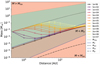 |
Fig. 8 Same as Fig. 5 but excluding the diffusive widening of the planetesimal ring. |
| In the text | |
|
Fig. 9 Same as Fig. 5 but for filaments around a 0.3 M⊙ mass star (top) and around a 0.1 M⊙ mass star (bottom). |
| In the text | |
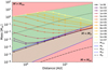 |
Fig. 10 Same as Fig. 5 but including the accretion of pebbles of τpeb = 0.1 onto the embryo. |
| In the text | |
|
Fig. 11 Total mass of the embryo (solid), the mass budget of planetesimals accreted (dashed), and mass of accreted pebbles (dotted). |
| In the text | |
|
Fig. 12 Same as Fig. 10 but for pebbles with a Stokes number of τs = 0.03 (top); mass of the embryo (bottom) considering the accretion of pebbles with τs = 0.1 (solid) and τs = 0.03 (dashed). |
| In the text | |
|
Fig. 13 Time required for the embryo to reach the transition mass for the nominal simulations without pebble accretion (solid) when considering the time-dependent pebble flux (dashed) and the fixed pebble flux (dotted) for different stellar masses (colour). The blue-shaded region refers to the time after which the gas surface density is reduced by half. |
| In the text | |
|
Fig. 14 Same as Fig. 13 but for the following setups: nominal (black), with a reduced initial embryo mass (yellow), reduced filament metallicity (red), and ignoring diffusion (magenta). |
| In the text | |
|
Fig. 15 Transition timing (colour) for the grid simulations around a 1 M⊙ mass star as a function of two grid dimensions, where the last variable not plotted is given by the bold value in Table 1. The grey area refers to simulations where the initial embryo is already larger than the transition mass. |
| In the text | |
|
Fig. 16 Transition timing of the grid at different stellar masses and separations where Fpeb = 100 M⊕/Myr and Mem = 1 Mem,0. |
| In the text | |
|
Fig. A.1 Growth track of a moon-mass embryo at 5 AU in our model (blue) and (Guilera et al. 2014) with only the local collisions (red) and the multi-annulus case (green). |
| In the text | |
|
Fig. A.2 Surface density distribution of the planetesimals at the location of the planet calculated using our model (blue) and the model presented in Guilera et al. (2014) with only the local collisions (red) and the multi-annulus case (green). |
| In the text | |
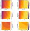 |
Fig. C.1 Same as Fig. 15 but for a 0.3M⊙ (left) and a 0.1M⊙ (right) mass star. |
| In the text | |
Current usage metrics show cumulative count of Article Views (full-text article views including HTML views, PDF and ePub downloads, according to the available data) and Abstracts Views on Vision4Press platform.
Data correspond to usage on the plateform after 2015. The current usage metrics is available 48-96 hours after online publication and is updated daily on week days.
Initial download of the metrics may take a while.