| Issue |
A&A
Volume 666, October 2022
|
|
|---|---|---|
| Article Number | A108 | |
| Number of page(s) | 12 | |
| Section | Planets and planetary systems | |
| DOI | https://doi.org/10.1051/0004-6361/202244333 | |
| Published online | 18 October 2022 | |
Growing the seeds of pebble accretion through planetesimal accretion
1
Centre for Star and Planet Formation, Globe Institute, University of Copenhagen,
Øster Voldgade 5-7,
1350
Copenhagen, Denmark
e-mail: sebastian.lorek@sund.ku.dk
2
Lund Observatory, Department of Astronomy and Theoretical Physics, Lund University,
Box 43,
221 00
Lund, Sweden
Received:
23
June
2022
Accepted:
1
August
2022
We explore the growth of planetary embryos by planetesimal accretion up to and beyond the point at which pebble accretion becomes efficient at the so-called Hill-transition mass. Both the transition mass and the characteristic mass of planetesimals that formed by the streaming instability increase with increasing distance from the star. We developed a model for the growth of a large planetesimal (embryo) embedded in a population of smaller planetesimals formed in a filament by the streaming instability. The model includes in a self-consistent way the collisional mass growth of the embryo, the fragmentation of the planetesimals, the velocity evolution of all involved bodies, and the viscous spreading of the filament. We find that the embryo accretes all available material in the filament during the lifetime of the protoplanetary disc only in the inner regions of the disc. In contrast, we find little or no growth in the outer parts of the disc beyond 5-10 AU. Overall, our results demonstrate very long timescales for collisional growth of planetesimals in the regions of the protoplanetary disc in which giant planets form. This means that in order to form giant planets in cold orbits, pebble accretion must act directly on the largest bodies present in the initial mass function of planetesimals with little or no help from mutual collisions.
Key words: methods: numerical / planets and satellites: formation
© S. Lorek and A. Johansen 2022
 Open Access article, published by EDP Sciences, under the terms of the Creative Commons Attribution License (https://creativecommons.org/licenses/by/4.0), which permits unrestricted use, distribution, and reproduction in any medium, provided the original work is properly cited.
This article is published in open access under the Subscribe-to-Open model. Subscribe to A&A to support open access publication.
1 Introduction
The classic picture for the formation of planets requires growth over several orders of magnitude in size. Starting from micrometre-sized dust and ice grains, coagulation produces millimetre-sized pebbles. Collisional and dynamical processes, such as bouncing, fragmentation, and radial drift, limit the maximum particle size (Blum & Wurm 2008; Güttler et al. 2010; Zsom et al. 2010; Krijt et al. 2015), and the formation of larger bodies is effectively prevented. Porosity in combination with an increased stickiness of ice could bypass these barriers (Wada et al. 2009; Okuzumi et al. 2012; Kataoka et al. 2013). However, it requires that ice is indeed stickier than rocky material (Gundlach & Blum 2015; Arakawa & Krijt 2021; Schräpler et al. 2022), which might not necessarily be the case (Musiolik & Wurm 2019; Kimura et al. 2020), and that the initial grains are sub-micron in size.
An alternative mechanism that has been extensively studied since its discovery invokes the concentration of pebbles through streaming instability and the subsequent gravitational collapse of dense filament-like structures that converts about millimetre-sized pebbles directly to about kilometre-sized planetesimals (e.g. Youdin & Goodman 2005; Johansen et al. 2007, 2014; Simon et al. 2016; Schäfer et al. 2017; Abod et al. 2019). These planetesimals then would grow to planet-sized bodies through runaway and oligarchic growth.
Runaway growth occurs when a planetesimal that is slightly more massive than the rest of the bodies accretes more efficiently through gravitational focusing. The mass ratio of the two bodies then increases with time, and the more massive body quickly outgrows the other planetesimals. As the growing body becomes more massive, it starts to gravitationally stir the surrounding planetesimals, which reduces gravitational focusing, and runaway growth ceases (Ida & Makino 1993; Kokubo & Ida 1996; Ormel et al. 2010). Eventually, a number of planetary embryos form that grow in an oligarchic fashion by accreting the plan-etesimals in their respective feeding zones until they reach their isolation mass (Kokubo & Ida 1998, 2000). In the final assembly of planets, these bodies grow by collisions, and when they reach a threshold mass of ~10 M⊕, they start to accrete gas from the surrounding nebula to form the terrestrial and giant planets.
Planetesimal accretion has long been thought to be the main pathway of planet formation. However, accretion is only efficient when the planetesimals are small. For small planetesimals of the order of a few kilometres in size at most, gas drag damps eccentricities and inclinations, boosting the accretion rate. However, it is uncertain whether planetesimals actually formed small or if they were large to begin with, typically around 100 km in diameter (Morbidelli et al. 2009; Weidenschilling 2011; Johansen et al. 2015). Evidence for the latter case is seen not only in the size distribution of the asteroid belt (Bottke et al. 2005) and in the cold classical Kuiper belt objects (Kavelaars et al. 2021), which are most likely the unaltered remnants of the planetesimals that formed in the outer Solar System, but also in the absence of large craters on Pluto, which indicates a lack of bodies ≲1 to 2 km in diameter (Singer et al. 2019). Furthermore, numerical studies of planetesimal formation through the streaming instability indicate a large initial size (Youdin & Goodman 2005; Johansen et al. 2007). The fragmentation of dense pebble filaments into planetesimals results in an initial mass function (IMF) of planetesimals that is well described by a power law with exponential cut-off for bodies exceeding a characteristic mass.
The characteristic mass translates into a characteristic size of ~ 100 km at a heliocentric distance of the asteroid belt, and the largest bodies that form through this process are roughly the size of Ceres (!10−4 Μ⊕; Simon et al. 2016; Schäfer et al. 2017; Abod et al. 2019; Li et al. 2019).
Because of the long timescales for planetesimal accretion, an efficient formation of terrestrial planets and the cores of giant planets within the lifetime of the protoplanetary disc of typically only a few million years (Haisch et al. 2001) is problematic. Johansen & Bitsch (2019) explored the conditions for forming the cores of the giant planets through planetesimal accretion. Their model focused on the growth track of a single migrating protoplanet sweeping through a population of planetesimals. They found that their fiducial model with constraints from the Solar System of (i) a primordial population of planetesimals of a few hundred Earth masses, (ii) a characteristic planetesimal size of ~ 100 km, and (iii) a weakly turbulent protoplanetary disc allow protoplanets to grow to only ~0.1 Μ⊕ within the disc lifetime of 3 Myr. Allowing for a massive disc of planetesimals of ~ 1000 Μ⊕ produces close-in giant planets, but fails to form cold giant planets, such as Jupiter or Saturn in the Solar System, unless the planetesimal size and turbulence strength are reduced at the same time. The conclusion of Johansen & Bitsch (2019) was that unless all three constraints are ignored, planetesimal accretion is insufficient to grow the cores of giant planets.
In contrast, fast growth can be achieved by the accretion of pebbles that are ubiquitous in the protoplanetary disc. Processes such as the streaming instability that explain planetesimal formation would convert between ~ 10% and up to 80% of the pebble mass trapped in filaments into planetesimals (Abod et al. 2019). The remnant pebbles as well as newly forming pebbles in the outer disc, where growth timescales are longer, would then provide a mass reservoir for further growth through pebble accretion. Pebble accretion becomes efficient for sufficiently large embryos above the so-called transition mass (Lambrechts & Johansen 2012), at which the growth mode changes from slow Bondi accretion to fast Hill accretion. The transition mass is ~2 × 10⁻³ Μ⊕ at 1 AU and ~6 × 10⁻³ Μ⊕ at 10 AU (Ormel & Klahr 2010; Lambrechts & Johansen 2012). Such a body then accretes a large number of pebbles within a short timescale and can form the terrestrial planets and the cores of the giant planets, consistent with the lifetime of protoplanetary discs (Lambrechts & Johansen 2012, 2014; Johansen & Lambrechts 2017; Johansen et al. 2021). However, a body of ~ 10−3 to 10−2 Μ⊕ needs to form in the first place, and planetesimal accretion could be the process for this.
In this paper, we investigate whether and under which conditions planetesimal accretion would lead to the formation of pebble-accreting embryos. Most simplified models that were developed to describe the growth of planets start with a narrow annulus of uniformly distributed planetesimals and an embryo in the centre. The growth of the embryo is followed until all planetesimals from the feeding zone are accreted (e.g. Thommes et al. 2003; Chambers 2006; Fortier et al. 2013). It is commonly assumed that there is only one planetesimal size, that the embryo mass follows from the transition from runaway to oligarchic growth, and that the feeding zone of the embryo is always populated with planetesimals. In our model, we wish to deviate in some aspects from this approach. While we also model the growth of an embryo embedded in a population of planetesimals, we employ a different initial situation where we (i) limit the available mass at a certain location by assuming that it is given by the mass budget of a streaming instability filament and (ii) use the streaming instability IMF to derive the characteristic planetesimal size and the size of the embryo. We furthermore deviate from the approach of Johansen & Bitsch (2019) by (i) ignoring migration, (ii) including fragmentation, and (iii) treating the growth rates and the eccentricity and inclination evolution of embryos, planetesimals, and fragments self-consistently. In this way, we study the growth from planetesimals to planetary embryos, while Johansen & Bitsch (2019) focused on the later growth stages in which migration is important.
Liu et al. (2019) investigated the growth from planetesimals to embryos and beyond through planetesimal and pebble accretion at the water snowline by means of N-body simulations. They tested different initial conditions for the planetesimal population of (i) a mono-dispersed population of planetesimals, (ii) a poly-dispersed population with IMF from streaming instability simulations, and (iii) a two-component population emerging from runaway growth of planetesimals. They find that a mono-dispersed population of planetesimals with a size of 400 km fails to form planets because growth timescales are too long due to the rapid excitation of eccentricities and inclinations of the planetesimals. In the other two cases, however, the largest body that forms, either because of the IMF or as a result of runaway growth of 100 km sized planetesimals, grows to several Earth masses firstly by planetesimal accretion and later through pebble accretion when the embryo reaches a mass of ~10−3 to 10−2 Μ⊕. Our work is complementary to their study because we explore the planetesimal accretion phase at various locations, whereas Liu et al. (2019) focused on a single site, the snowline at 2.7 AU.
The paper outline is as follows. In Sect. 2, we outline our model and our assumptions. In Sect. 3, we present the results of planetesimal accretion around a solar-like star, which is our fiducial model. In Sect. 4, we explore and discuss parameter variations of the fiducial model. Finally, in Sect. 5 we summarise and conclude the study.
2 Methods
2.1 Basic outline
We used a semi-analytic model to follow the growth of a planetary embryo at a fixed distance r from the central star (e.g. Chambers 2006). Three different types of bodies were considered. These are (i) an embryo, (ii) a population of planetesimals, and (iii) a population of fragments.
The embryo was treated as a single body with mass Μem, radius Rem, eccentricity eem, inclination iem, and surface density Σem. For the surface density of the embryo, we simply assumed that the mass of the embryo was distributed uniformly in an annulus of area Aem centred at r with a width of brh,

where rh = r (Μem/3Μ⊙))1/3 is the Hill radius (Chambers 2006). The value b = 10 corresponds to the typical spacing of isolated embryos, which has been shown in N-body simulations to be ~10 Hill radii (Kokubo & Ida 1998).
A single planetesimal has mass mp and radius Rp, and the population has a surface density Σp. We took the root-mean-square eccentricity and inclination to describe the orbits of the planetesimals. The fragments were treated in the same way as the planetesimals with a mass mfr and radius Rfr for a single fragment, and a surface density Σfr, root-mean-square eccentricity, and inclination for the population.
2.2 Mass and surface density evolution, fragmentation
The embryo grows by accreting planetesimals and fragments. The accretion rate of the embryo can be written as

where stands for either planetesimals or fragments. Furthermore, we have the reduced mutual Hill radius hem,k = ((Mem + mk) / (3 M⊙))1/3, the Keplerian frequency ΩK, and a dimensionless collision rate Pcol that is a function of the sizes of the colliding bodies, and their mutual eccentricities and inclinations (Inaba et al. 2001; Chambers 2006).
We are now able to formulate the evolution equations for the surface densities. For the embryo surface density, we differentiate Eq. (1) with respect to time and obtain

for the change of surface density due to the accretion of bodies from population k.
To derive the evolution of planetesimal and fragment surface densities, we first need to derive the number of fragments that is produced in a collision between planetesimals. To do this, we first calculated the number of collisions per unit time between planetesimals,

where Ns,p = Σp/mp is the surface number density of planetesimals and Pcol is the collision rate between planetesimals (Inaba et al. 2001). Initially, there are no fragments. When planetesimals are excited to a high enough eccentricity, such that evK ≈ vesc, collisions become disruptive and fragments are produced. Typically, this results in a collisional cascade with a size distribution of fragments, but here we used a typical fragment size of 0.5 km to represent the fragment population. The fragmentation model of Kobayashi & Tanaka (2010) allowed us to determine the total mass of fragments ∆Mfr that is produced in a disruptive collision between two planetesimals. The value of ∆Mfr depends on the ratio of impact energy and material-dependent critical disruption energy of the planetesimals. By multiplying the collision rate of planetesimals with ∆Mfr, we obtain the mass production rate of fragments,

Our approach was to keep the total mass of solids constant, that is, we have the condition

where the total mass of planetesimals Mp is given by ΣpAp, where Ap = 2πr∆r is the area of the annulus of width ∆r that the planetesimals occupy, and likewise for the fragments. The initial width of the annulus is ηr (see below) for planetesimals and fragments, but the annuli widen diffusively with time because eccentricities and inclinations are excited by viscous stirring (Ohtsuki & Tanaka 2003; Tanaka et al. 2003).
With the assumption of constant total mass, we can now formulate the evolution equations for the surface densities given the mass accretion rate of the embryo  and the production rate of fragments by taking the time derivative of Eq. (6), which gives

Substituting the total mass changes with surface densities and areas, we obtain that the surface density of planetesimals reduces due to accretion of planetesimals by the embryo and due to fragmentation,

The area ratio appears because of the mass conservation condition. Likewise, the surface density of fragments evolves according to

The set of Eqs. (3), (4), (5), (8), and (9) fully describes the mass growth of the embryo and the conversion of planetesimals into fragments.
We emphasise that the embryo does not grow to the isolation mass in the classical sense by accreting all the material in the expanding feeding zone. Instead, growth is limited by the available mass contained in the annulus of width ∆r. We considered this approach suitable for studying the growth of an embryo in an isolated filament formed through streaming instability where a fixed amount of mass is converted into planetesimals in a confined narrow ring. Furthermore, while the embryo grows by the accretion of planetesimals and fragments, the mass distribution of planetesimals and fragments does not evolve over time owing to our choice of representing these populations by bodies of a characteristic mass.
2.3 Velocity evolution
The velocity distributions, that is, the eccentricities and inclinations, of the bodies evolve through viscous stirring and dynamical friction. To take this into account, we used the rate equations from Ohtsuki et al. (2002) for the root-mean-square eccentricities and inclinations. We included viscous stirring and dynamical friction between all populations with the exception that the single embryo did not interact with itself. Gas drag dampens the orbits of the bodies, and we included damping for the embryo, the planetesimals, and the fragments (Adachi et al. 1976; Inaba et al. 2001). We did not include turbulent stirring of planetesimals through the disc gas.
2.4 Protoplanetary disc
We used the self-similar solution for a viscously evolving α-disc (Shakura & Sunyaev 1973; Lynden-Bell & Pringle 1974). The disc is heated by stellar irradiation with a temperature profile of

(Ida et al. 2016). The viscously heated part ofthe disc would initially extend to ~5 AU for our fiducial parameter choices (Ida et al. 2016). However, we neglected viscous heating here (i) because recent work indicates that irradiation rather than viscous heating might be the relevant heat source for protoplanetary discs (Mori et al. 2019, 2021), and (ii) because we verified by running a model with a viscous temperature profile where it applies that the choice of temperature profile has negligible impact on the planetesimal accretion process studied here. The filament mass (see Sect. 2.6) and the initial radii of planetesimals and embryos (see Sect. 2.7) vary only within a factor of unity, which does not affect the results.
The viscosity in the α-disc model is  , where we used α = 10−2. The value of α determines the viscous evolution timescale of the disc and the accretion of the gas onto the star. The value is consistent with what is determined from observations of protoplanetary discs (Hartmann et al. 1998). For the temperature profile used here, the viscosity is a power law in radial distance, ν ∝ rγ, with an exponent of γ = 15/14.
The surface density profile of the self-similar solution for a power-law viscosity is
![${\sum _{{\rm{gas}}}}{\rm{ = }}{{{{\dot M}_{ \star 0}}} \over {3\pi {v_1}}}{\left( {{r \over {{r_1}}}} \right)^{ - \gamma }}\tau \left( {5/2 - \gamma } \right)/\left( {2 - \gamma } \right)\exp \left[ { - {1 \over \tau }{{\left( {{r \over {{r_1}}}} \right)}^{2 - \gamma }}} \right],$](/articles/aa/full_html/2022/10/aa44333-22/aa44333-22-eq13.png)
where  is the characteristic time for the viscous evolution, τ = (t/tvis) + 1, r1 is the characteristic radius of the disc, and ν1 = v(r1) is the viscosity at distance r1. For the initial mass accretion rate, we used
  at 0.5 Myr, which corresponds to a typical class II object (Hartmann et al. 1998, 2016). The total disc mass was set to be 10% of the stellar mass, and by integrating the surface density at t = 0 from the inner edge of the disc, which we set to 0.1 AU, to infinity, we can determine the characteristic disc radius, which is ~72 AU in our fiducial case.
2.5 Formation time of planetesimals and embryo
Our model started at time t0 when planetesimals are expected to have formed. To estimate t0, we assumed that the planetesimal accretion phase takes place in the class-II phase of the disc, ~0.5 Myr after star formation (Evans et al. 2009; Williams & Cieza 2011).
To form planetesimals, dust first grows by coagulation to pebbles. The growth timescales  of the dust is

where ∈g ≈ 0.5 is a coagulation efficiency and Z is the solid-togas ratio of the dust in the disc (Birnstiel et al. 2012; Lambrechts & Johansen 2014). The time for grains of radius R0 to grow to pebbles of radius Rpeb is found to be

(Lambrechts & Johansen 2014). Dust growth is limited by radial drift and fragmentation (Birnstiel et al. 2012), and we used the minimum of both for the pebbles. The fragmentation-limited Stokes numberis

where we set the collision velocity of similar-sized pebbles driven by turbulence (Ormel & Cuzzi 2007) equal to the fragmentation threshold velocity vfrag. The value of vfrag ranges from ~ 1 m s−1 for silicate pebbles (Blum & Wurm 2008) to ~ 10 m s−1 for icy pebbles (Gundlach & Blum 2015). However, more recent studies have shown that ice might not be as sticky as previously thought (e.g. Musiolik & Wurm 2019; Kimura et al. 2020) and that the tensile strength of ice aggregates is comparable to the tensile strength of silicates (Gundlach et al. 2018). We therefore used a common fragmentation threshold velocity of vfrag = 1 ms−1 for fragmentation-limited growth in our study. The turbulent collision velocity depends on the midplane turbulence at, which is different from the gas a that drives the viscous evolution of the protoplanetary disc. The value of at obtained from observations of the dust component of protoplanetary discs ranges from ~10−5 to a few times 10−4 (Pinte et al. 2016; Villenave et al. 2022). We decided to use a value of αt = 10−4 in our study.
In the drift-limited case, the Stokes number is

which is obtained from setting the growth timescale of the pebbles (Eq. (12)) equal to the drift timescale tdrift = r/vr, with vr = 2ηvKτs being the radial velocity of the pebbles.
The pebbles are subsequently concentrated by the streaming instability and form planetesimals through the gravitational collapse of dense particle filaments. Depending on the size of the pebbles that form, the streaming instability takes about ten (for large pebbles, τs = 0.3) to a few thousand (for small pebbles, τs ≈ 10−3−10−2) local orbital periods to create dense filaments that subsequently fragment gravitationally into planetesimals (Yang & Johansen 2014; Yang et al. 2017; Li et al. 2018, 2019). We calculated the pebble growth time at distance r according to Eq. (13) and the streaming instability timescale as  and added both to the 0.5 Myr to obtain the initial time t0 for our simulations.
2.6 Filament mass
The initial conditions of the planetesimal population are derived in the framework of planetesimal formation through the streaming instability. We assumed that the streaming instability forms a dense filament of pebbles which fragments into planetesimals. The typical radial width of a filament is ~ηr, where η is related to the pressure gradient of the disc gas and r is the distance from the star (Yang & Johansen 2014; Liu et al. 2019; Gerbig et al. 2020). This length scale can be thought of as the length scale over which the Keplerian flow adjusts to the gas flow. We set the solid-to-gas ratio in the filament to Zfil = 0.1, and the mass contained in one filament is therefore Mfil = 2πrΣgasZfll ηr (Liu et al. 2019). Because not all pebbles are converted into planetesimals, we introduced a planetesimal formation efficiency peff. The total mass of planetesimals is then peff Mfil (Liu et al. 2019). For an optimistic upper limit on embryo growth, we assumed peff = 1 throughout the study. Figure 1 shows the mass of the filaments as a function of distance for different stellar masses.
2.7 Initial masses of planetesimals and embryo
The initial sizes of planetesimals and embryos follow from the IMF found in streaming instability simulations. The IMF is a power law with an exponential cut-off above a characteristic mass,
![${{{N_ > }\left( m \right)} \over {{N_{{\rm{tot}}}}}} = {\left( {{m \over {{m_{\min }}}}} \right)^{ - p}}\exp \left[ {{{\left( {{{{m_{\min }}} \over {{m_{\rm{p}}}}}} \right)}^q} - {{\left( {{m \over {{m_{\rm{p}}}}}} \right)}^q}} \right]$](/articles/aa/full_html/2022/10/aa44333-22/aa44333-22-eq22.png)
(Schäfer et al. 2017). The slope of the power law was p ≈ 0.6 and the steepness of the cut-off was q ≈ 0.4 (Simon et al. 2016; Schäfer et al. 2017). The IMF is top heavy, which means that most of the mass is in the large bodies of characteristic mass. We used the characteristic mass above which the IMF drops exponentially as a proxy for the planetesimal mass, which is

where  and h is the aspect ratio of the disc (Liu et al. 2020). To determine the mass of the embryo, we calculated the mass of the single most massive body that forms from the IMF. To do this, we set N>(m) = 1 in Eq. (16) and solved for m. The value of Ntot was found by noting that the total number of bodies are determined by the smallest bodies. We set the minimum mass to mmin = 10−3 mp and calculated Ntot = Mfil/mmin. Figure 2 shows the initial mass and size of the embryo and the planetesimals as a function of distance for different stellar masses.
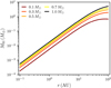 |
Fig. 1 Total mass of filaments formed through streaming instability. The mass of the filament Mfil = 2πrΣgasΖfilηr increases with distances from ≲10−3 Μ⊕ in the inner disc to almost 10 Μ⊕ in the outer disc. Mfil is the maximum mass the embryo can obtain by accreting planetesimals. The filament masses for different stellar masses are colour-coded. |
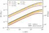 |
Fig. 2 Initial masses of planetesimals and embryos. We show the mass of planetesimals (solid) and embryos (dashed) at initial time t0, which ranges from ~0.5 Myr in the inner disc to ~1.5 Myr in the outer disc. The planetesimal size is the characteristic size, which follows from the streaming instability IMF, and the embryo size is the single most massive body. The initial sizes for different stellar masses are colour-coded. |
Fiducial simulation parameters.
2.8 Diffusion of planetesimals and fragments
We included the diffusive widening of the planetesimal and fragment rings due to viscous stirring (Ohtsuki & Tanaka 2003; Tanaka et al. 2003). This reduced the surface densities with time which impacts both the accretion and the stirring rates. We assumed that the initial width of ηr increases with time as  , where D is the diffusion coefficient and t is the time, as it is characteristic for a random walk (Liu et al. 2019). The diffusion coefficient is related to the viscous stirring rates of eccentricity and inclination (Ohtsuki & Tanaka 2003; Tanaka et al. 2003).
3 Results
In the fiducial model, we used a solar-mass central star with a viscously evolving disc heated by solar irradiation. We placed filaments at various distances ranging from 0.1 to 100 AU and simulated the growth of the embryo for 10 Myr. Table 1 summarises the model parameters. We later varied the stellar mass, the solid-to-gas ratio of the filament, and other parameters to explore how they affect the growth of the embryo.
3.1 Growth of the embryo
Figure 3 shows how the embryo mass evolves with time as a function of distance. The time snapshots are relative to the initial time t0 of the simulation, which ranged from ~0.5 Myr in the inner disc to ~ 1.5 Myr in the outer disc. The planetesimal size increased with distance, and the initial mass of the embryo was typically a factor 102 to 103 higher than the planetesimal mass, as shown in Fig. 2. Inside ~2 AU, the growth timescale is short and embryos reach their final mass by accreting all the available mass in the filament within 10 Myr. Farther out, growth slows down and ceases to almost zero for ≳20 AU.
The reasons for the rapid growth inside ~2 AU are the high surface density of planetesimals, which results in a short growth timescale, and the excitation of the eccentricities of the planetesimals, which results in fragmentation and the boost of growth through accretion of fragments. This is visible in Fig. 4, which shows the time evolution of the surface densities of the planetesimals and the fragments and the eccentricity evolution of the planetesimals in the middle and bottom panels for various distances. The eccentricity at which the collision speed exceeds the escape speed of the planetesimal is approximately given by

where we set the random speed of the planetesimals ~evK equal to their escape speed. The bottom panel in Fig. 4 shows that within ~2 AU, the embryo excites the planetesimals above the threshold in short times (≲ 104 yr). As a consequence, the embryo efficiently accretes the small fragments (which we assumed here to have a constant radius of 0.5 km). However, in the outer disc, this effect is negligible because planetesimal eccentricities are not excited enough to result in fragmentation. For example, at 5 AU and for 200 km planetesimals (see Fig. 2), this requires eccentricities ≳2 × 10⁻², which are reached only after ~1 Myr (after t0) and later. Therefore, fragmentation, if at all, sets in late and embryo growth is not boosted by fragment accretion as is the case in the inner disc. At even larger distances, fragmentation plays no role because the stirring of planetesimals by the embryo and by self-stirring is not sufficient to reach eesc. Therefore, the long accretion timescale limits the growth in the outer disc.
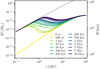 |
Fig. 3 Embryo mass at different distances for different time snapshots around a 1 M⊙ star. The embryo mass is shown for different times (relative to t0) as coloured lines. Accretion efficiency decreases with increasing distance and almost ceases outside of ~20 AU. The maximum mass Mfil that an embryo can reach (dotted black line) is over-plotted. |
3.2 Eccentricity evolution
Figure 5 shows the eccentricities of embryos, planetesimals, and fragments as a function of distance for different times. Initially, embryos and planetesimals have the same eccentricity and inclination such that e = η/2 and i/e =1/2 because we assumed that just after formation there has not been enough time for dynamical friction to result in a mass dependent eccentricity. The initial eccentricity of the fragments was set to 10% of the escape speed of a planetesimal.
3.2.1 Planetesimals
In the inner disc, the eccentricity of the planetesimals is determined by the equilibrium of viscous stirring by the embryo and gas drag because the gas density is sufficiently high. The damping timescale for gas drag is

where mp and Rp are mass and radius of the planetesimal, ρgas is the gas density, and Cd is the drag coefficient (Adachi et al. 1976; Inaba et al. 2001). The timescale on which viscous stirring of planetesimals by an embryo of mass Mem and surface density Σem excites eccentricities is given by

(Ida & Makino 1993). When viscous stirring by the embryo and gas drag on the planetesimal are in equilibrium, the eccentricity can be calculated by setting the damping timescale equal to the stirring timescale,

(Thommes et al. 2003). The drag coefficient can be assumed to be 2, which is valid for planetesimal-sized bodies. The typical spacing of embryos b is of the order of 10 Hill radii (Kokubo & Ida 1998) and enters via the embryo surface density Σem = Mem/(2πrbrh). Figure 2 shows that the mass of planetesimals and embryos scales with distance approximately as mp ∝ r3/2. Because of the distance dependence of mp and ρgas, Tdrag ∝ r47/14 (for our viscous α-disc) increases strongly with distance and the equilibrium eccentricity increases with distance approximately as eeq ∝ r61/70, which is the slope of e with r, as shown in Fig. 5 inside of ~0.8 AU.
In the outer disc, damping by gas drag becomes inefficient because of the lower gas density and because of the large planetesimals. Therefore, viscous stirring by the embryo is the process that determines the planetesimal eccentricity. The viscous stirring of planetesimals by the embryo is expressed as

(Ida & Makino 1993). Inserting Eq. (20), we can integrate Eq. (22), which gives

where Tvis,0 is the viscous stirring timescale for initial planetesimal eccentricity e0. Figure 4 shows that e ∝ t1/4 for large distances, that is, outside of ~2 AU. Evaluating the scaling with distance, we find that e ∝ r1/4, when taking the r dependency of the embryo mass (initial mass because there is some growth up to ~20 AU) and of the initial eccentricity (∝ r4/7 because η ∝ (cs/vK)2) into account. However, Fig. 5 shows a more flat scaling with r. The reason is that even though the eccentricity evolution is determined by viscous stirring because the damping timescale is too long to result in equilibrium eccentricities, gas drag still damps the eccentricities.
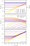 |
Fig. 4 Embryo mass, surface densities, and planetesimal eccentricity as function of time at different distances. The different panels are (top) embryo mass, (middle) surface densities of planetesimals (solid) and fragments (dashed), and (bottom) planetesimal eccentricity and threshold eccentricity for fragmentation (dashed). Time is expressed relative to the planetesimal formation time t0 for better comparison. The colours correspond to the different distances. |
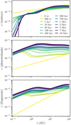 |
Fig. 5 Eccentricities of embryos, planetesimals, and fragments at different distances for different times. The different panels show the eccentricities of the embryo (top), the planetesimals (middle), and the fragments (bottom). The eccentricities are shown for different times (relative to t0) as coloured lines. In the inner disc, the bodies follow the equilibrium eccentricity given by the balance of viscous stirring through the embryo and friction with the gas. In the outer disc, eccentricities are determined by viscous stirring with minor damping from gas drag. |
3.2.2 Fragments
The eccentricities of the fragments within ~1 AU are given by the equilibrium eccentricity. Because fragments are smaller, they are more strongly damped by the gas and hence acquire lower eccentricities. The ratio of fragment size to planetesimal size is ~10−2 close to the star, which translates into a ratio of eeq to ~0.4, as shown in Fig. 5. In the outer disc, eccentricities are excited by viscous stirring and damped by gas drag, where equilibrium values might be reached at late times.
3.2.3 Embryo
The eccentricity of the embryo is more complex, as shown in Fig. 5, because it is determined through the interplay of viscous stirring through the planetesimals, dynamical friction from planetesimals and fragments, and damping through gas drag. The mass growth further complicates the picture, and simple scaling arguments as provided for planetesimals and fragments no longer suffice. However, qualitatively, the embryo keeps a low eccentricity (≲ 10−3) throughout the simulation. Close to the star, the high gas and planetesimal surface density in combination with the fast growth circularises the orbit. In the outer disc, where no growth occurs, the embryo eccentricity remains close to the initial value experiencing some damping through gas drag and dynamical friction.
4 Discussion
4.1 Varying the stellar mass
The stellar mass affects the mass accretion rate  , the luminosity L⋆, and the density and temperature structure of the disc.
Here, we investigate the growth of embryos around different stellar masses, ranging from 0.1 M⊙ to 1 M⊙. The mass accretion rate of low-mass stars is also lower. Manara et al. (2012) provided a fit for the mass accretion rate as a function of stellar age and mass. For our chosen initial time of 0.5 Myr, we find  . Hartmann et al. (2016) reported that the mass accretion rate correlates with stellar mass as
  . The linear scaling of Manara et al. (2012), with
  , results in smaller and more rapidly evolving discs than the quadratic scaling. We ran simulations with both relations to scale the initial mass accretion rate of 10−7 M⊙ yr−1 for = 1 M⊙ to lower stellar masses. The luminosity scales with mass as
  for stellar ages ≲ 10 Myr (Liu et al. 2020), and hence we set the slope of the L⋆-M⋆-relation to an intermediate value of 1.5.
Figure 6 shows the final embryo mass at 10 Myr as a function of distance for different stellar masses for  . We find that the maximum distance out to which embryos accrete all available mass of the filament scales with stellar mass, ranging from ~0.3 AU for a M⋆ = 0.1 M⊙ to ~ 1 AU for a M⋆+ = 1 M⊙. Farther out, accretion becomes less efficient and ceases for distances ≳10 AU for = 0.1 M⊙ and ≳30 AU for M⋆ = 1 M⊙. In comparison to the quadratic scaling, the final embryo masses for
  are shown in Fig. 7. The general finding is the same as for Fig. 6, but the embryos are more massive for all stellar masses <1 M⊙. The reason for this is that
  . For the shallower scaling, the discs around the lower mass stars have higher surface densities and hence the masses of the filaments are higher, which consequently leads to higher masses of embryos and more mass that is available for the embryos to accrete.
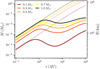 |
Fig. 6 Final sizes of embryos for different stellar masses. The embryo mass after 10 Myr is shown as a function of distances for different stellar masses (colour-coded). We used the quadratic scaling |

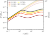 |
Fig. 7 Final sizes of embryos for different stellar masses. The embryo mass after 10 Myr is shown as a function of distances for different stellar masses (colour-coded). We used the linear scaling |

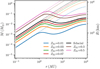 |
Fig. 8 Final sizes of embryos for different filament solid-to-gas ratios. The embryo mass after 10 Myr is shown as a function of distances for a 1 M⊙ star for different values of Zfil (coloured lines). The fiducial case (solid black line) as well as the filament mass (dotted lines) are shown for comparison. |
4.2 Varying the filament solid-to-gas ratio
Figure 8 shows the outcome of our model for different values of the filament solid-to-gas ratio. This Ζfil provides a minimum value for how much pebble mass is turned into planetesimals (assuming that the planetesimal formation efficiency is 100%, which we used in our model). We varied Ζfil from the canonical value of Ζfil = 0.01 to Ζfil = 0.5, which means that the mass in planetesimals would be 50% of the gas mass at distance r. We find that varying the value of Ζfil does not change the general picture of efficient growth for distances ≲1 to 2 AU. The final embryo masses vary according to the value of Zfil simply because the filaments are more massive.
4.3 Reducing the initial embryo mass
In the fiducial run and variations thereof, we used the single most massive body from the streaming instability IMF as the embryo. In this case, the embryo is typically a factor 103 more massive than the planetesimals (see Fig. 2). We ran a model in which we reduced the embryo mass by a factor of 10 while keeping the total mass of the filament fixed. The mass ratio of embryo to planetesimals is hence ~ 10 to 100. Figure 9 shows that reducing the initial mass of the embryo does not change the final outcome for ≲3 AU, where the embryo accretes nearly all the available mass. Outside ~3AU, however, accretion efficiency decreases and for ≳20 AU, the embryo does not grow significantly.
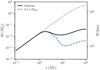 |
Fig. 9 Final sizes of embryos for reduced initial embryo mass. The embryo mass after 10 Myr is shown as a function of distances for a 1 M⊙ star for a 10 times lower initial embryo mass (blue line). The fiducial case (black line) as well as the filament mass (dotted line) are shown for comparison. |
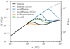 |
Fig. 10 Final sizes of embryos for different parameter variations. The embryo mass after 10 Myr is shown as a function of distances for a 1 M⊙ star for different cases (coloured lines) of no fragmentation, no diffusive widening, and fixed zero fragment eccentricity. The fiducial case (solid black line) as well as the filament mass (black dotted line) are shown for comparison. |
4.4 Fragmentation, eccentricities, and diffusive widening
Figure 10 compares the final masses of embryos for models, where we set the fragment eccentricity and inclination to zero, disabled fragmentation, disabled diffusive widening of the planetesimal and fragment rings, or extended the simulation from 10 Myr to 1 Gyr.
Disabling fragmentation results in longer growth timescales. The final mass of the embryo after 10 Myr, however, is not strongly affected. Inside of ~ 1 AU, we find the same final mass while between ~ 1 and ~5 AU, the final mass is lower by less than a factor of 2 at most. Outside ~5 AU, we find the same final mass as in the fiducial case because fragmentation does not play a role.
The eccentricity of the fragments affects the growth behaviour more strongly. Fixing the fragments on orbits with zero eccentricity and inclination (i.e. assuming that gas drag is very efficient) allows the embryo to accrete fragments at a constant rate in the low-velocity regime (Inaba et al. 2001; Chambers 2006), while in the fiducial case, the accretion rate decreases as fragments are excited by viscous stirring through the embryo and the planetesimals. As a consequence, we find that the embryos are more massive than in the fiducial case out to distances of ~20 AU. We also ran a model in which we set the eccentricity and inclination of the embryo to zero. In this case, we did not find any significant deviation from the fiducial run. We conclude that a circular and planar embryo orbit as used in other studies (e.g. Chambers 2006) is a valid approximation because the eccentricity of the embryo is ~10−3≪ep,efr because of dynamical friction and gas drag (Fig. 5).
Lastly, we considered the diffusive widening of the planetesimal and fragment rings. Disabling diffusion has a strong impact on embryo growth. Within 10 Myr and out to ~5 AU, the embryo accretes all the filament mass, which allows growth to up to ~0.2 M⊕. On much longer timescales than 10 Myr, embryos would grow up to ~ 1M⊕ out to ~20 AU. This is shown in Fig. 10, in which we show the final mass after 1 Gyr for the fiducial and the no-diffusion case for comparison. Without diffusion, embryos grow up to ~1 M⊕, whereas with diffusion, the mass even after 1 Gyr is ~0.1 M⊕ at most. The reason for the strongly enhanced growth without diffusive widening is that the surface densities of planetesimals and fragments decrease only through accretion. However, the increase in eccentricities and inclinations through viscous stirring causes the bodies to occupy a larger volume, which additionally reduces the surface density and hence reduces the accretion rate of the embryo, which is proportional to the surface density of the accreted bodies.
4.5 Implications for pebble accretion
The growth of embryos by planetesimal accretion in the filaments formed through streaming instability is efficient only in the inner part of the protoplanetary disc. In the inner disc, the collision timescale is short enough and fragmentation of planetesimals is efficient enough for an embryo to accrete all the available material. At larger distances and especially outside ~5 to 10 AU, planetesimal accretion is highly inefficient, even though the available material in the filament increases. The larger sizes of the planetesimals, the excitation of planetesimal eccentricities, and the lack of fragmentation prevents embryos from growing massive within the lifetime of the disc of 10 Myr.
The inefficient growth by planetesimal accretion does not necessarily imply that planets cannot form at all. We did not consider pebble accretion in our model because we focused on the accretion of the filament material turned into planetesimals. However, embryos might still be able to reach masses for which pebble accretion becomes an highly efficient growth process. Pebble accretion becomes important when the friction time of the pebbles is shorter than the time in which they would pass by the embryo (Ormel 2017). This condition leads to the onset mass for pebble accretion
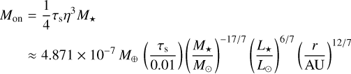
(Visser & Ormel 2016; Ormel 2017). Above the so-called transition mass, pebble accretion becomes very efficient. The transition mass marks the change from drift-driven (Bondi) accretion to shear-driven (Hill) accretion of pebbles (Lambrechts & Johansen 2012; Johansen & Lambrechts 2017; Ormel 2017). This means that in the latter case, pebbles from the entire Hill sphere are accreted by the embryo. The transition mass can be found by equating the Bondi radius rB = GMem/(ηvK)2 and the Hill radius, and it reads

(Ormel 2017). Pebble accretion stops when the embryo reaches the pebble isolation mass. At this mass, the embryo carves a gap in the gas disc that creates a pressure bump outside its orbit, which stops pebbles from drifting inward and being accreted by the embryo. The pebble isolation mass is

which is derived from fits to hydrodynamic simulations of pebble accretion (Bitsch et al. 2018).
We now compare the embryo masses to the characteristic masses for the pebble accretion given above. Figure 11 shows a map in which we highlight the different regimes of pebble accretion. For an embryo to accrete pebbles efficiently, the mass needs to be above the transition mass. Below the transition mass and above the onset mass, embryos would still be able to accrete pebbles, but on the less efficient Bondi branch. Figure 11 shows that the initial embryo mass is below the transition mass for all stellar masses; even though the difference is small for M⋆ = 1 Μ⊙. For M⋆ = 0.1 M⊙, the initial embryo mass is even below the onset mass for distances ≳2 AU. For M* = 0.3 M⊙, the initial embryo mass is below the onset mass outside of ~50 AU. Figure 11 also shows that the maximum mass an embryo can reach through planetesimal accretion in a filament (the filament mass Μfil) is above the transition mass (except for the M⋆ = 0.1 Μ⊙ outside ~20 AU), but well below the pebble isolation mass, which means that enough mass in planetesimals would be available for embryos to grow into the pebble-accreting regime. However, we find that embryos growing through accretion of planetesimal would reach the transition mass only out to a distance of ~20 AU for a solar-like central star within the lifetime of a protoplanetary disc. For stars of lower mass, this distance shifts significantly inwards to ≲1 AU for M⋆ = 0.1 Μ⊙. Therefore, we conclude that planetesimal accretion might be a channel for forming the seeds for pebble accretion out to ~20 AU. Farther out, where planetesi-mal accretion becomes negligible, pebble accretion even though on the slow Bondi branch would be the only growth channel. Our result agrees with Liu et al. (2019), who investigated the growth of planetesimals to planets at a single site, namely the water snowline at 2.7 AU, through planetesimal and pebble accretion using N-body simulations. In their work, embryos would also grow to masses of 10−3 to 10−2 M⊕ through planetesimal accretion, after which pebble accretion would take over. The final embryo masses in our model at 2.7 AU (Fig. 3 and the bottom right panel of Fig. 11) show comparable masses.
4.6 Limitations of the model
Our model describes the growth of an embryo at a fixed location. We neglected the migration of the embryo, the planetesi-mals, and the fragments for several reasons: (i) For the embryo masses considered here (≲0.1 M⊕), the migration timescales are some million years and longer (Tanaka et al. 2002; Cresswell & Nelson 2008; Ida et al. 2020), (ii) in addition to a more complicated model, radial drift of planetesimals and fragments would only reduce the accretion efficiency due to an additional drain of available material, and (iii) gas-drag-induced radial drift peaks for metre-sized bodies, but planetesimals, fragments, and embryos have sizes of one kilometre to several hundreds of kilometres, resulting in slow radial drift. Therefore, the non-migrating bodies provide an upper limit on the final masses. Any migration would result in bodies with lower mass.
In our study, we did not assume that streaming instability forms filaments at special locations in the disc, such as snowlines, where a pressure bump would naturally lead to an increased solid-to-gas ratio due to pile-up of pebbles that would trigger the streaming instability (Drazkowska & Alibert 2017; Schoonenberg et al. 2018). Instead, we studied what would happen if filaments occurred at any location (Carrera et al. 2017; Lenz et al. 2019). A consequence of this would be a significant reservoir of planetesimals that are not accreted. This reservoir can nevertheless interact with the planets that might form by pebble accretion, leading to scattering and populating of the Kuiper belt, scattered disc, and Oort cloud, thus providing the bodies for comets and Kuiper belt objects (Brasser & Morbidelli 2013). The fact that outside of 10 AU neither significant growth nor fragmentation occurs might imply that the size distribution of the planetesimals remains also largely unchanged. The cold-classical Kuiper belt might be a remnant of this. In our model, the total mass of planetesimals in the whole disc is ~333 M⊕. The mass contained in the asteroid belt region between 2 AU and 4 AU is ~10 M⊕, and in the region of the primordial disc region between 15 AU and 30 AU it is ~50 M⊕, both of which are orders of magnitude higher than the current mass in asteroids and in the Kuiper belt, which are estimated to be 4 × 10⁻⁴ M⊕ and ~10−2 M⊕, respectively (DeMeo & Carry 2013; Fraser et al. 2014). Therefore, efficient depletion becomes necessary, such as the giant planet instability in the Nice model, which could have been responsible for sculpturing the outer Solar System and depleting the asteroid belt by scattering of planetesimals and ejection of planetesimals from the Solar System (Gomes et al. 2005; Tsiganis et al. 2005; Morbidelli 2010; Brasser & Morbidelli 2013). On the other hand, we assumed that 100% of the filament mass is converted into planetesimals, which gives an upper limit on the available mass. The planetesimal formation efficiencies in streaming instability simulations are not well constrained and can vary significantly from ≲10% to as high as ~80% (Abod et al. 2019). Converting fewer pebbles into planetesimals will reduce the available mass significantly, and additionally, lifting the assumption that filaments form throughout the disc reduces the amount of planetesimals even further.
We furthermore neglected interactions of filaments with each other and that especially the large embryos in the outer disc whose Hill radii might exceed the typical spacing of the filaments would be able to accrete from neighbouring filaments. However, the relevance of this might be low because even though there is a huge mass reservoir of planetesimals of several Earth masses, the embryos accrete almost no planetesimals.
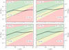 |
Fig. 11 Mapping final regimes of embryo masses to pebble accretion. The figure shows the masses of the embryos at 10 Myr for four different stellar masses as a function of distance. The initial masses (dashed lines) and the filament masses (dotted lines) are shown for comparison. Where the mass is below the onset mass Mon (Eq. (24)) or above the pebble isolation mass Miso (Eq. (26)), pebble accretion would be absent (red area). Above the onset mass but below the transition mass Mtr (Eq. (25)), embryos would accrete pebbles on the Bondi branch (yellow area). Efficient pebble accretion would be possible for embryo masses above Mtr (green). |
5 Conclusion
We modelled the planetesimal accretion phase that follows the birth of planetesimals. To do this, we developed a model for the growth of a large planetesimal (embryo) embedded in a population of smaller planetesimals of characteristic size. The model included mass growth of the embryo, the fragmentation of planetesimals, and the velocity evolution of all involved bodies in a self-consistent fashion. We represented the planetesimal size distribution at birth with bodies of characteristic masses, the planetesimals and the embryo. Our growth model hence described an oligarchic-like growth. Fragmentation assumed a representative fragment size. We found that embryos accrete the available material efficiently only in the inner disc where a combination of high planetesimal surface density and fragmentation ensures short growth timescales for the embryo. On the other hand, we find little to no growth in the outer parts of the disc beyond ~5 to 10 AU on a 10 Myr timescale. The embryos typically reached masses in the range ~10−3 to 10−1 M⊕. When we compared the embryo masses to the transition mass for pebble accretion, we found that embryos would be able to grow into the pebble-accreting regime through planetesimal accretion out to ~20 AU. Pebble accretion on the less efficient Bondi branch might help embryos to reach the transition mass also beyond ~20 AU.
Acknowledgements
We thank the anonymous referee for a constructive feedback that contributed in improving the quality of our work. A.J. is supported by the Swedish Research Council (Project Grant 2018-04867), the Danish National Research Foundation (DNRF Chair grant DNRF159), and the Knut and Alice Wallenberg Foundation (Wallenberg Academy Fellow Grant 2017.0287). A.J. further thanks the European Research Council (ERC Consolidator Grant 724 687-PLANETESYS), the Göran Gustafsson Foundation for Research in Natural Sciences and Medicine, and the Wallenberg Foundation (Wallenberg Scholar KAW 2019.0442) for research support.
References
- Abod, C. P., Simon, J. B., Li, R., et al. 2019, ApJ, 883, 192 [Google Scholar]
- Adachi, I., Hayashi, C., & Nakazawa, K. 1976, Progr. Theor. Phys., 56, 1756 [Google Scholar]
- Arakawa, S., & Krijt, S. 2021, ApJ, 910, 130 [NASA ADS] [CrossRef] [Google Scholar]
- Birnstiel, T., Klahr, H., & Ercolano, B. 2012, A&A, 539, A148 [NASA ADS] [CrossRef] [EDP Sciences] [Google Scholar]
- Bitsch, B., Morbidelli, A., Johansen, A., et al. 2018, A&A, 612, A30 [NASA ADS] [CrossRef] [EDP Sciences] [Google Scholar]
- Blum, J., & Wurm, G. 2008, ARA&A, 46, 21 [Google Scholar]
- Bottke, W. F., Durda, D. D., Nesvorný, D., et al. 2005, Icarus, 175, 111 [Google Scholar]
- Brasser, R., & Morbidelli, A. 2013, Icarus, 225, 40 [Google Scholar]
- Carrera, D., Gorti, U., Johansen, A., & Davies, M. B. 2017, ApJ, 839, 16 [Google Scholar]
- Chambers, J. 2006, Icarus, 180, 496 [NASA ADS] [CrossRef] [Google Scholar]
- Cresswell, P., & Nelson, R. P. 2008, A&A, 482, 677 [NASA ADS] [CrossRef] [EDP Sciences] [Google Scholar]
- DeMeo, F. E., & Carry, B. 2013, Icarus, 226, 723 [NASA ADS] [CrossRef] [Google Scholar]
- DraZkowska, J., & Alibert, Y. 2017, A&A, 608, A92 [CrossRef] [EDP Sciences] [Google Scholar]
- Evans, Neal J. I., Dunham, M. M., Jørgensen, J. K., et al. 2009, ApJS, 181, 321 [NASA ADS] [CrossRef] [Google Scholar]
- Fortier, A., Alibert, Y., Carron, F., Benz, W., & Dittkrist, K. M. 2013, A&A, 549, A44 [NASA ADS] [CrossRef] [EDP Sciences] [Google Scholar]
- Fraser, W. C., Brown, M. E., Morbidelli, A., Parker, A., & Batygin, K. 2014, ApJ, 782, 100 [Google Scholar]
- Gerbig, K., Murray-Clay, R. A., Klahr, H., & Baehr, H. 2020, ApJ, 895, 91 [CrossRef] [Google Scholar]
- Gomes, R., Levison, H. F., Tsiganis, K., & Morbidelli, A. 2005, Nature, 435, 466 [Google Scholar]
- Gundlach, B., & Blum, J. 2015, ApJ, 798, 34 [Google Scholar]
- Gundlach, B., Schmidt, K. P., Kreuzig, C., et al. 2018, MNRAS, 479, 1273 [NASA ADS] [CrossRef] [Google Scholar]
- Güttler, C., Blum, J., Zsom, A., Ormel, C. W., & Dullemond, C. P. 2010, A&A, 513, A56 [Google Scholar]
- Haisch, Karl E. J., Lada, E. A., & Lada, C. J. 2001, ApJ, 553, L153 [NASA ADS] [CrossRef] [Google Scholar]
- Hartmann, L., Calvet, N., Gullbring, E., & D’Alessio, P. 1998, ApJ, 495, 385 [Google Scholar]
- Hartmann, L., Herczeg, G., & Calvet, N. 2016, ARA&A, 54, 135 [Google Scholar]
- Ida, S., & Makino, J. 1993, Icarus, 106, 210 [NASA ADS] [CrossRef] [Google Scholar]
- Ida, S., Guillot, T., & Morbidelli, A. 2016, A&A, 591, A72 [NASA ADS] [CrossRef] [EDP Sciences] [Google Scholar]
- Ida, S., Muto, T., Matsumura, S., & Brasser, R. 2020, MNRAS, 494, 5666 [Google Scholar]
- Inaba, S., Tanaka, H., Nakazawa, K., Wetherill, G. W., & Kokubo, E. 2001, Icarus, 149, 235 [CrossRef] [Google Scholar]
- Johansen, A., & Bitsch, B. 2019, A&A, 631, A70 [NASA ADS] [CrossRef] [EDP Sciences] [Google Scholar]
- Johansen, A., & Lambrechts, M. 2017, Annu. Rev. Earth Planet. Sci., 45, 359 [Google Scholar]
- Johansen, A., Oishi, J. S., Mac Low, M.-M., et al. 2007, Nature, 448, 1022 [Google Scholar]
- Johansen, A., Blum, J., Tanaka, H., et al. 2014, in Protostars and Planets VI, eds. H. Beuther, R. S. Klessen, C. P. Dullemond, & T. Henning, 547 [Google Scholar]
- Johansen, A., Mac Low, M.-M., Lacerda, P., & Bizzarro, M. 2015, Sci. Adv., 1, 1500109 [CrossRef] [Google Scholar]
- Johansen, A., Ronnet, T., Bizzarro, M., et al. 2021, Sci. Adv., 7, eabc0444 [NASA ADS] [CrossRef] [Google Scholar]
- Kataoka, A., Tanaka, H., Okuzumi, S., & Wada, K. 2013, A&A, 557, L4 [NASA ADS] [CrossRef] [EDP Sciences] [Google Scholar]
- Kavelaars, J. J., Petit, J.-M., Gladman, B., et al. 2021, ApJ, 920, L28 [NASA ADS] [CrossRef] [Google Scholar]
- Kimura, H., Wada, K., Kobayashi, H., et al. 2020, MNRAS, 498, 1801 [Google Scholar]
- Kobayashi, H., & Tanaka, H. 2010, Icarus, 206, 735 [NASA ADS] [CrossRef] [Google Scholar]
- Kokubo, E., & Ida, S. 1996, Icarus, 123, 180 [Google Scholar]
- Kokubo, E., & Ida, S. 1998, Icarus, 131, 171 [Google Scholar]
- Kokubo, E., & Ida, S. 2000, Icarus, 143, 15 [Google Scholar]
- Krijt, S., Ormel, C. W., Dominik, C., & Tielens, A. G. G. M. 2015, A&A, 574, A83 [NASA ADS] [CrossRef] [EDP Sciences] [Google Scholar]
- Lambrechts, M., & Johansen, A. 2012, A&A, 544, A32 [NASA ADS] [CrossRef] [EDP Sciences] [Google Scholar]
- Lambrechts, M., & Johansen, A. 2014, A&A, 572, A107 [NASA ADS] [CrossRef] [EDP Sciences] [Google Scholar]
- Lenz, C. T., Klahr, H., & Birnstiel, T. 2019, ApJ, 874, 36 [NASA ADS] [CrossRef] [Google Scholar]
- Li, R., Youdin, A. N., & Simon, J. B. 2018, ApJ, 862, 14 [NASA ADS] [CrossRef] [Google Scholar]
- Li, R., Youdin, A. N., & Simon, J. B. 2019, ApJ, 885, 69 [NASA ADS] [CrossRef] [Google Scholar]
- Liu, B., Ormel, C. W., & Johansen, A. 2019, A&A, 624, A114 [NASA ADS] [CrossRef] [EDP Sciences] [Google Scholar]
- Liu, B., Lambrechts, M., Johansen, A., Pascucci, I., & Henning, T. 2020, A&A, 638, A88 [EDP Sciences] [Google Scholar]
- Lynden-Bell, D., & Pringle, J. E. 1974, MNRAS, 168, 603 [Google Scholar]
- Manara, C. F., Robberto, M., Da Rio, N., et al. 2012, ApJ, 755, 154 [NASA ADS] [CrossRef] [Google Scholar]
- Morbidelli, A. 2010, Comptes Rendus Physique, 11, 651 [NASA ADS] [CrossRef] [Google Scholar]
- Morbidelli, A., Bottke, W. F., Nesvorný, D., & Levison, H. F. 2009, Icarus, 204, 558 [Google Scholar]
- Mori, S., Bai, X.-N., & Okuzumi, S. 2019, ApJ, 872, 98 [NASA ADS] [CrossRef] [Google Scholar]
- Mori, S., Okuzumi, S., Kunitomo, M., & Bai, X.-N. 2021, ApJ, 916, 72 [NASA ADS] [CrossRef] [Google Scholar]
- Musiolik, G., & Wurm, G. 2019, ApJ, 873, 58 [NASA ADS] [CrossRef] [Google Scholar]
- Ohtsuki, K., & Tanaka, H. 2003, Icarus, 162, 47 [NASA ADS] [CrossRef] [Google Scholar]
- Ohtsuki, K., Stewart, G. R., & Ida, S. 2002, Icarus, 155, 436 [Google Scholar]
- Okuzumi, S., Tanaka, H., Kobayashi, H., & Wada, K. 2012, ApJ, 752, 106 [NASA ADS] [CrossRef] [Google Scholar]
- Ormel, C. W. 2017, Astrophysics and Space Science Library, The Emerging Paradigm of Pebble Accretion, eds. M. Pessah, & O. Gressel, 445, 197 [NASA ADS] [CrossRef] [Google Scholar]
- Ormel, C. W., & Cuzzi, J. N. 2007, A&A, 466, 413 [NASA ADS] [CrossRef] [EDP Sciences] [Google Scholar]
- Ormel, C. W., & Klahr, H. H. 2010, A&A, 520, A43 [NASA ADS] [CrossRef] [EDP Sciences] [Google Scholar]
- Ormel, C. W., Dullemond, C. P., & Spaans, M. 2010, ApJ, 714, L103 [NASA ADS] [CrossRef] [Google Scholar]
- Pinte, C., Dent, W. R. F., Ménard, F., et al. 2016, ApJ, 816, 25 [Google Scholar]
- Schäfer, U., Yang, C.-C., & Johansen, A. 2017, A&A, 597, A69 [Google Scholar]
- Schoonenberg, D., Ormel, C. W., & Krijt, S. 2018, A&A, 620, A134 [NASA ADS] [CrossRef] [EDP Sciences] [Google Scholar]
- Schräpler, R. R., Landeck, W. A., & Blum, J. 2022, MNRAS, 509, 5641 [Google Scholar]
- Shakura, N. I., & Sunyaev, R. A. 1973, A&A, 24, 337 [NASA ADS] [Google Scholar]
- Simon, J. B., Armitage, P. J., Li, R., & Youdin, A. N. 2016, ApJ, 822, 55 [Google Scholar]
- Singer, K. N., McKinnon, W. B., Gladman, B., et al. 2019, Science, 363, 955 [NASA ADS] [CrossRef] [Google Scholar]
- Tanaka, H., Takeuchi, T., & Ward, W. R. 2002, ApJ, 565, 1257 [Google Scholar]
- Tanaka, H., Ohtsuki, K., & Daisaka, H. 2003, Icarus, 161, 144 [NASA ADS] [CrossRef] [Google Scholar]
- Thommes, E. W., Duncan, M. J., & Levison, H. F. 2003, Icarus, 161, 431 [NASA ADS] [CrossRef] [Google Scholar]
- Tsiganis, K., Gomes, R., Morbidelli, A., & Levison, H. F. 2005, Nature, 435, 459 [Google Scholar]
- Villenave, M., Stapelfeldt, K. R., Duchêne, G., et al. 2022, ApJ, 930, 11 [NASA ADS] [CrossRef] [Google Scholar]
- Visser, R. G., & Ormel, C. W. 2016, A&A, 586, A66 [NASA ADS] [CrossRef] [EDP Sciences] [Google Scholar]
- Wada, K., Tanaka, H., Suyama, T., Kimura, H., & Yamamoto, T. 2009, ApJ, 702, 1490 [Google Scholar]
- Weidenschilling, S. J. 2011, Icarus, 214, 671 [NASA ADS] [CrossRef] [Google Scholar]
- Williams, J. P., & Cieza, L. A. 2011, ARA&A, 49, 67 [Google Scholar]
- Yang, C.-C., & Johansen, A. 2014, ApJ, 792, 86 [Google Scholar]
- Yang, C. C., Johansen, A., & Carrera, D. 2017, A&A, 606, A80 [NASA ADS] [CrossRef] [EDP Sciences] [Google Scholar]
- Youdin, A. N., & Goodman, J. 2005, ApJ, 620, 459 [Google Scholar]
- Zsom, A., Ormel, C. W., Güttler, C., Blum, J., & Dullemond, C. P. 2010, A&A, 513, A57 [NASA ADS] [CrossRef] [EDP Sciences] [Google Scholar]
All Tables
All Figures
|
Fig. 1 Total mass of filaments formed through streaming instability. The mass of the filament Mfil = 2πrΣgasΖfilηr increases with distances from ≲10−3 Μ⊕ in the inner disc to almost 10 Μ⊕ in the outer disc. Mfil is the maximum mass the embryo can obtain by accreting planetesimals. The filament masses for different stellar masses are colour-coded. |
| In the text | |
|
Fig. 2 Initial masses of planetesimals and embryos. We show the mass of planetesimals (solid) and embryos (dashed) at initial time t0, which ranges from ~0.5 Myr in the inner disc to ~1.5 Myr in the outer disc. The planetesimal size is the characteristic size, which follows from the streaming instability IMF, and the embryo size is the single most massive body. The initial sizes for different stellar masses are colour-coded. |
| In the text | |
|
Fig. 3 Embryo mass at different distances for different time snapshots around a 1 M⊙ star. The embryo mass is shown for different times (relative to t0) as coloured lines. Accretion efficiency decreases with increasing distance and almost ceases outside of ~20 AU. The maximum mass Mfil that an embryo can reach (dotted black line) is over-plotted. |
| In the text | |
|
Fig. 4 Embryo mass, surface densities, and planetesimal eccentricity as function of time at different distances. The different panels are (top) embryo mass, (middle) surface densities of planetesimals (solid) and fragments (dashed), and (bottom) planetesimal eccentricity and threshold eccentricity for fragmentation (dashed). Time is expressed relative to the planetesimal formation time t0 for better comparison. The colours correspond to the different distances. |
| In the text | |
|
Fig. 5 Eccentricities of embryos, planetesimals, and fragments at different distances for different times. The different panels show the eccentricities of the embryo (top), the planetesimals (middle), and the fragments (bottom). The eccentricities are shown for different times (relative to t0) as coloured lines. In the inner disc, the bodies follow the equilibrium eccentricity given by the balance of viscous stirring through the embryo and friction with the gas. In the outer disc, eccentricities are determined by viscous stirring with minor damping from gas drag. |
| In the text | |
|
Fig. 6 Final sizes of embryos for different stellar masses. The embryo mass after 10 Myr is shown as a function of distances for different stellar masses (colour-coded). We used the quadratic scaling |
| In the text | |
|
Fig. 7 Final sizes of embryos for different stellar masses. The embryo mass after 10 Myr is shown as a function of distances for different stellar masses (colour-coded). We used the linear scaling |
| In the text | |
|
Fig. 8 Final sizes of embryos for different filament solid-to-gas ratios. The embryo mass after 10 Myr is shown as a function of distances for a 1 M⊙ star for different values of Zfil (coloured lines). The fiducial case (solid black line) as well as the filament mass (dotted lines) are shown for comparison. |
| In the text | |
|
Fig. 9 Final sizes of embryos for reduced initial embryo mass. The embryo mass after 10 Myr is shown as a function of distances for a 1 M⊙ star for a 10 times lower initial embryo mass (blue line). The fiducial case (black line) as well as the filament mass (dotted line) are shown for comparison. |
| In the text | |
|
Fig. 10 Final sizes of embryos for different parameter variations. The embryo mass after 10 Myr is shown as a function of distances for a 1 M⊙ star for different cases (coloured lines) of no fragmentation, no diffusive widening, and fixed zero fragment eccentricity. The fiducial case (solid black line) as well as the filament mass (black dotted line) are shown for comparison. |
| In the text | |
|
Fig. 11 Mapping final regimes of embryo masses to pebble accretion. The figure shows the masses of the embryos at 10 Myr for four different stellar masses as a function of distance. The initial masses (dashed lines) and the filament masses (dotted lines) are shown for comparison. Where the mass is below the onset mass Mon (Eq. (24)) or above the pebble isolation mass Miso (Eq. (26)), pebble accretion would be absent (red area). Above the onset mass but below the transition mass Mtr (Eq. (25)), embryos would accrete pebbles on the Bondi branch (yellow area). Efficient pebble accretion would be possible for embryo masses above Mtr (green). |
| In the text | |
Current usage metrics show cumulative count of Article Views (full-text article views including HTML views, PDF and ePub downloads, according to the available data) and Abstracts Views on Vision4Press platform.
Data correspond to usage on the plateform after 2015. The current usage metrics is available 48-96 hours after online publication and is updated daily on week days.
Initial download of the metrics may take a while.