| Issue |
A&A
Volume 696, April 2025
|
|
|---|---|---|
| Article Number | A138 | |
| Number of page(s) | 11 | |
| Section | Extragalactic astronomy | |
| DOI | https://doi.org/10.1051/0004-6361/202451206 | |
| Published online | 10 April 2025 | |
The MeerKAT Fornax Survey
V. H I kinematics and Fornax cluster membership of the dwarf galaxy ESO 358-60
1
Ruhr University Bochum, Faculty of Physics and Astronomy, Astronomical Institute (AIRUB), 44780 Bochum, Germany
2
INAF – Osservatorio Astronomico di Cagliari, Via della Scienza 5, I-09047 Selargius (CA), Italy
3
Netherlands Institute for Radio Astronomy (ASTRON), Oude Hoogeveensedijk 4, 7991 PD Dwingeloo, The Netherlands
4
Max-Planck-Institut für Radioastronomie, Auf dem Hügel 69, 53121 Bonn, Germany
5
Department of Physics and Electronics, Rhodes University, Artillery Road, Makhanda, 1640
South Africa
⋆ Corresponding author; This email address is being protected from spambots. You need JavaScript enabled to view it.
Received:
21
June
2024
Accepted:
6
March
2025
Abstract
Context. The MeerKAT Fornax Survey (MFS) is a large survey project mapping the H I in the Fornax cluster. Most of the cluster members detected in H I show significant signs of interaction with the intracluster medium or other galaxies. The galaxy ESO 358-60, however, stands out as its large H I disk appears regular and undisturbed. Combined with the fact that the galaxy’s systemic velocity is at the edge of the velocity distribution of Fornax, a possible explanation for this undisturbed disk is that the galaxy is not in Fornax.
Aims. Our goal is to understand the detailed morphology and kinematics of the H I disk of ESO 358-60 and, by doing so, establish whether the galaxy is a member of Fornax.
Methods. We analyzed the H I distribution within and around ESO 358-60 based on the MFS observations in a 2 deg2 field around the galaxy. We visually inspected the low resolution data in order to study the H I disk from the center to its outskirts and look for low column density gas that could reveal recent interactions. We then constructed a detailed parameterization of the H I disk by fitting a tilted ring model to the high resolution data cube. Using a bootstrap method, we established accurate errors on our best-fit models. We used the fitted rotational velocity to place the galaxy on the baryonic Tully-Fisher relation. By equating the galaxy’s H I and 3.6 μm fluxes to the thus retrieved baryonic mass, we obtained a redshift-independent distance.
Results. We confirm that the immediate surroundings of ESO 358-60 are quiescent relative to other MFS detections and find no obvious companion interacting with the galaxy. Our modeling confirms the regularity of the H I disk in ESO 358-60 but also shows that the galaxy’s H I distribution contains a significant line-of-sight warp and that radial motions, on the order of 10 km s−1, cover the extent of the optical disk. From the modeling we obtain a velocity Vflat = 48.1 ± 1.4 km s−1 for the best-fit rotation curve. This leads to a distance from the baryonic Tully-Fisher relation of 9.4 ± 2.5 Mpc which is ∼10 Mpc less than the distance to the Fornax cluster. This distance fits better not only with Vflat but also with the overall rotation curves and H I content of low mass galaxies and the fact that the galaxy appears undisturbed and reasonably symmetric. It is also consistent with the distance calculated in the Cosmicflows project. At 9.4 Mpc, ESO 358-60 cannot be a member of the Fornax cluster; it is instead a foreground field galaxy.
Key words: ISM: kinematics and dynamics / ISM: structure / galaxies: distances and redshifts / galaxies: evolution / galaxies: ISM / galaxies: kinematics and dynamics
© The Authors 2025
 Open Access article, published by EDP Sciences, under the terms of the Creative Commons Attribution License (https://creativecommons.org/licenses/by/4.0), which permits unrestricted use, distribution, and reproduction in any medium, provided the original work is properly cited.
This article is published in open access under the Subscribe to Open model. This email address is being protected from spambots. You need JavaScript enabled to view it. to support open access publication.
1. Introduction
The Fornax cluster is one of the nearest clusters (D = 20 ± 0.3 ± 1.4 Mpc; Blakeslee et al. 2009), which makes it an excellent target to study the effects of the cluster environment on the neutral hydrogen content of its members. This cluster has a high central surface density of galaxies (Ferguson 1989) but a rather low mass (Mvir = 5 × 10¹³ M⊙; Drinkwater et al. 2001) and might represent an environment bridging massive groups and clusters. The MeerKAT Fornax Survey (MFS; Serra et al. 2023) mapped its 21 cm emission to determine the gas distribution and kinematics in this unique environment. As the gas content of cluster galaxies is highly skewed toward gas-poor galaxies (Dressler 1980; Kleiner et al. 2023), it is crucial to establish cluster membership for the relatively few galaxies detected in H I.
The galaxy ESO 358-60 is an irregular dwarf galaxy that appears edge-on in the optical (see Fig. 1; de Vaucouleurs et al. 1991). It has a diffuse and fairly uniform surface brightness (Matthews & Gallagher 1997) and is forming stars at a low rate (Leroy et al. 2019). Table 1 provides an overview of several of its parameters. It is classified as a likely member of the Fornax cluster (FCC 302; Ferguson 1989) following the morphological criteria developed by Binggeli et al. (1985) for determining membership to the Virgo cluster. In the absence of systemic velocities, for irregular galaxies, these criteria are “resolution into knots” of stellar associations and H II regions and adherence to the “surface brightness” versus absolute magnitude relation (Binggeli et al. 1984) in the faint end. These criteria are mostly considered for the removal of background galaxies since for Virgo only a small number or no foreground galaxies are expected (Binggeli et al. 1985). It is not clear how well these criteria exclude foreground galaxies, and Ferguson (1989) did not address this when establishing the original membership designations.
Properties of ESO 358-60.
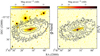 |
Fig. 1. Left: g-band optical image from the Fornax Deep Survey (FDS; Iodice et al. 2016; Venhola et al. 2018) overlaid with intensity contours of the H I (see Fig. 2). Right: Far-ultraviolet image from GALEX observations overlaid with velocity contours extracted from the 21 cm observations (Fig. 2). The blue circle marks what appears to be a large star-forming region. |
ESO 358-60 stands out from other H I detections in the MFS due to its low systemic velocity (vsys = 804 km s−1; Schröder et al. 2001) and the fact that it does not display signs of tidal interaction or an H I tail (Serra et al. 2023). Its H I disk is significantly more extended than its observed stellar disk (Fig. 1), and it is difficult to reconcile this apparently unaffected disk with the galaxy traveling through the intracluster medium (ICM) of the Fornax cluster at a speed of ≥600 km s−1. In fact, if we assume the ICM density is ∼4 × 10⁻⁵ cm−3 at the projected distance of ESO 358-60 (Chen et al. 2007) and approximate an outer stellar surface brightness of ∼0.4 M⊙ pc−2 (∼10% of the surface brightness at R80; Bouquin et al. 2018) and an outer gas surface brightness of 0.4 M⊙ pc−2 (this work), following the prescription from Gunn & Gott (1972), we find a ratio of ram pressure to restoring force of ∼100. This ratio is far too high for the gas disk of the galaxy to remain unaffected by the ram pressure.
One possible explanation for these peculiarities would be that ESO 358-60 is not part of the Fornax cluster. Its low systemic velocity does not exclude it immediately as a Fornax member as the difference with the systemic velocity of the cluster center (vsys = 1454 km s−1; Maddox et al. 2019) is slightly more than two times the velocity dispersion of the cluster (σFornax = 286 km s−1; Maddox et al. 2019). Therefore, taking advantage of the extremely regular morphology and kinematics of the H I disk (Sect. 2), we performed an in-depth investigation of the neutral hydrogen in this galaxy in order to place it on the baryonic Tully-Fisher relation (BTFR; Tully & Fisher 1977; McGaugh et al. 2000; Lelli et al. 2019). Due to its low scatter, the BTFR can be used to obtain the baryonic mass of the galaxy based solely on its rotational velocity. This mass can then be equated to the mass obtained from the flux of the stellar and gas components to calculate a distance independent of redshift (Tully & Fisher 1977).
This paper is structured as follows. In Sect. 2 we present and discuss the H I data that we used to obtain a tilted ring model (TRM) and investigate the surroundings of ESO 358-60, and Sect. 3 explains how we obtained the TRM. In Sect. 4 we derive a distance based on the BTFR and compare it to other distance indicators, in Sect. 5 we present and discuss the presence of radial motions in this galaxy, and in Sect. 6 we summarize our findings.
2. Data
The H I data used in this study were observed as part of the MFS. For the tilted ring modeling, we focused on the highest resolution data cube for ESO 358-60. We used the lower resolution data products solely to obtain an impression of the H I environment of the galaxy at the end of this section. For the details of the data reduction and the lower resolution product we refer to Serra et al. (2023).
For ESO 358-60 the high resolution data cube has a spatial resolution of 12.2″ × 9.6″ full width at half maximum (FWHM), a velocity resolution of 1.4 km s−1 and a noise level of 0.24 mJy beam−1 in a channel (nH I = 4 × 1019 cm−2 for 3σ over a 25 km s−1 line width). This is lower than the average noise across the full mosaic (σfull = 0.3 mJy beam−1; Serra et al. 2023) but within the expected variations of the noise level across the MFS footprint. The cube is in a barycentric spectroscopic frame and all velocities cited in this paper follow the optical definition.
Figure 2 shows the moment 0 and moment 1 map of the data cube and Fig. 3 the global line profile. Already by visually inspecting these maps several obvious implications can be drawn for the distribution and kinematics of the H I in this galaxy. The central surface brightness distribution is highly elongated indicating an edge-on disk or a bar like distribution in the center. The outer parts are much more circular and thus point to a lower inclination. The surface brightness distribution in the approaching and receding sides appear largely symmetric and, except for a slight position angle (PA) warp in the receding side, no major deviations from an elliptical distribution are visible. The peak of the H I emission coincides with a large star-forming region, indicated by the blue circle in Fig. 1, just offset from the center of the galaxy. The galaxy does look somewhat disturbed in the optical but this is not unusual for an irregular galaxy. The most prominent disturbance lies on the eastern edge on the optical disk; just before the start of the PA warp in the receding side of the galaxy.
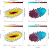 |
Fig. 2. Moment maps of the H I in the galaxy ESO 358-60. Dark gray contours show the data. The blue contours indicate the automatic model (in the top panels) and the best-fit model (in the bottom panels). Left: Moment 0 or integrated intensity map of the galaxy. Contours are at |

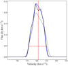 |
Fig. 3. Global line profile of ESO 358-60. The black line indicates the data, the blue the best-fit model, and the gray the automatic model. The vertical dashed red line indicates the systemic velocity, and the horizontal line the uncorrected W20. |
The velocity field shows a similar picture of regularity. The central major and minor axes are not perpendicular indicating the existence of radial motions in the galaxy. These motions appear to occur largely symmetrically around the morphological minor axis and cover the full extent of the optical disk. Besides these radial motions the velocity field appears regular and no major disturbances can be identified in this map nor in the cube directly.
We used the lower resolution products of the MFS to search for H I, which could indicate an interaction despite the regularity of the disk. Figure 4 shows the 2 deg2 surrounding ESO 358-60 and shows the relatively quiet immediate surroundings of the galaxy compared to other Fornax galaxies detected in H I. In fact, the only spectroscopically confirmed galaxy within ∼20′ (∼115 kpc at the distance of Fornax) is FCC 298, which is significantly offset in velocity (Vsys = 1620 km s−1). Within a 20’ radius there are six more dwarfs for which no redshift is observed (Venhola et al. 2018). These are all significantly redder (g′−r′ > 0.5) and fainter (mr′ > 17) than ESO 358-60 and their effective radius in the r′-band is always less than half (Reffr′ < 14″) that of ESO 358-60 (see Table 1). None of these dwarfs are detected in the MFS nor have they visibly affected the H I disk of ESO 358-60. The nearest galaxy detected in H I is NGC 1436, a lenticular galaxy for which the outer H I disk was stripped and the detected H I is well contained within the stellar disk (Loni et al. 2023). All other galaxies in Fig. 4 detected in H I show disturbed disks and tails and H I debris. It is these differences with its surrounding H I detections that have prompted us to question the cluster membership of ESO 358-60.
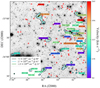 |
Fig. 4. g′-band image of the 2 deg2 surrounding ESO 358-60 from the FDS (Iodice et al. 2016; Venhola et al. 2018) overlaid with the lowest reliable contours (3σ) of the 98″ and 41″ resolutions of the MFS. For the 21″ resolution, we plot the contour corresponding to ∼1 M⊙ pc−2. The beams are displayed in the bottom-left corner. All galaxies that are spectroscopically confirmed in the field are labeled, and the background color of the label indicates the systemic velocity of the system. The color bar on the right shows the correspondence between color and velocity. Galaxies identified in the FDS, but not spectroscopically confirmed, are marked with a red x. |
As mentioned in the previous paragraph, in the cluster environment it is still possible to have a fairly regular disk that has had its outer edges stripped away by interactions (Chung et al. 2009; Loni et al. 2023). Therefore, as final check, we compared the H I diameter to the optical diameter. The ratio between these two diameters is 2.1, a ratio that is normal for field galaxies (Table 1; Broeils & Rhee 1997). This confirms that the H I of ESO 358-60 does not show significant distortions when compared to field galaxies.
3. Models
To obtain an initial TRM for the galaxy, we first ran PYFAT (v0.1.21; Kamphuis et al. 2015; Kamphuis 2024) on the data cube. The parameters of this automatic fit are shown in Fig. 5 as the gray lines and the non-radially varying parameters are listed in Table 2. Even though PYFAT divides the model into an approaching and receding side, the final preferred model is fully symmetric, reflecting the regularity and symmetry that made ESO 358-60 stand out in the first place. The moment 0 and 1 maps of the automated model are displayed as the blue contours in the top panels of Fig. 2. This model fits the data well within the parameters that are allowed to vary within PYFAT with a few exceptions. In the top left panel of Fig. 2 it can be seen that the model is too elongated compared to the data. This is due to a surface brightness that is too high in the outer rings and, even though a significant variation of the inclination (Δi ∼ 10°) is already incorporated in the model, an underestimation of the line-of-sight warp. Additionally, the radial motions are not fitted by PYFAT (see Fig. 2, top right) and need to be incorporated into the model manually. We therefore considered this model as a starting point and improved on it through guided fitting with TIRIFIC (Józsa et al. 2007).
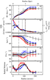 |
Fig. 5. Fitted parameters for the various models. Light gray lines represent the PYFAT model, black lines the single disk model, and the blue (approaching) and red (receding) lines the final best-fit model. The panels show the rotation velocities (a), surface brightness distribution (b), inclination (c), PA (d), and radial motions (e), all as function of radius. The vertical dot-dashed gray line indicates R25, and the vertical dashed lines in panel b mark where the surface brightness is equal to 1 M⊙ pc−2. |
Non-radially varying model parameters.
As the automatic fit is completely symmetric, we first reduced the model back to a single disk. After manually increasing the line-of-sight warping in the input parameters, we refit the model to the data. During the manual fitting, we grouped certain rings for several parameters, through TIRIFIC’s VARINDX parameter, to ensure a stable fit. The grouping varies between different parameters in order to reduce degeneracy within the fitting. For example, in the inclination we might group the rings 10 to 13 by only varying rings 10 and 13 and determining rings 11 and 12 through a non-rounded Akima interpolation with natural boundaries. In this case we would make sure that in the rotational velocities we fit either ring 11 or 12 and interpolated over rings 10 and 13 in order to counteract the degeneracy between these parameters in the fitting. If the outer most rings are not varied individually, we extrapolated by matching the ring value to the last fitted ring. We always ran TIRIFIC in a fitting mode and judged the quality of the model via a visual comparison between various representations of the data and the model. Between iterations we sometimes adjusted the limits manually in the input parameter file, but any final model is always the result of the χ2 minimization process with TIRIFIC.
Compared to the fitting philosophy of PYFAT, we made two changes to ensure the stability of the fitting when adding radial motions to the rings. Firstly, we fit the dispersion as a singular parameter. Secondly, we set the scale height of the model to the value found in the automatic fit.
After a few iterations it becomes clear that the required surface brightness of the outer rings should be so far below the noise of the data that they have no influence on the model anymore. Therefore, we cut the last two rings from the modeling. Once we deemed the outer warp to be well matched in the model, we added radial motions to the model.
This procedure led to a single disk best-fit model, the parameters of which are shown as the black lines in Fig. 5. However, after including the radial motions, we found that the H I distribution in the galaxy is not perfectly symmetric; it looked like the model can be improved by fitting the approaching and receding side independently. As such, we split the model into two disks again and refit this model in the same manner as the manual fits for the single disk. This leads to a final best-fit model of which the parameters are shown in Fig. 5 as the blue (approaching) and red (receding) lines. The bottom panels of Fig. 2 show the model overlaid on the moment maps and Fig. 6 a position-velocity (PV) diagram along the major axis.
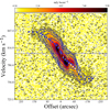 |
Fig. 6. PV diagram along the major axis. Gray contours and the color scale show the data, and blue contours show the best-fit model. Contours are at 1.5, 3, 6, 12, 24 × σ with σ = 0.24 mJy beam−1 (3.2 × 1018 cm−2 in a channel). The dashed gray line indicates the spatial fitted center, and the dashed colored line indicates the fitted systemic velocity of the best-fit model. The blue circles indicate the Vobs = Vrot × sin(i) of the best-fit model, and the white circles the same for the rising model (see text). To be concurrent with the right ascension, offsets are decreasing from left to right. |
This model fits the data remarkably well, as can be seen in the moment maps (Fig. 2, bottom panels, blue contours), and is our best-fit model. As in several smaller galaxies rotation curves (RCs) are observed to keep rising until their last measured point, we refit our best-fit model with TIRIFIC forcing a RC that continues to rise until the last point.
Visually comparing this model to the data shows that such a model deteriorates the match between the data and model in the outer rings. This is most clearly seen in the velocity field (Fig. 2, right bottom panel, white contours) where the outer contours are more open than the data. As such, we consider the RCs of the rising model as an absolute upper limit on the RC.
In the analysis that follows, we used the model with a flat outer RC where the approaching and receding side are fitted independently of each other, as this is the best-fit model. However, as the single disk model is mostly an average between the two sides (see Fig. 5) it makes little difference for the analysis of the galaxy as whole whether we use our best-fit model or the single disk model.
In the manual fitting we fit the dispersion as a singular value and have fixed the scale height. We do not expect the dispersion to affect the fitted rotational velocities, but the scale height could. The scale height we used is ∼0.4 kpc around 10 Mpc (see Table 2). This is typical for the inner parts of H I disks (O’Brien et al. 2010)2. However, H I disks are expected to flare significantly. If this is the case in ESO 358-60, we might underestimate the scale height in the outer parts of the model. In principle this can then lead to us underestimating the outer inclinations as the increased thickness of the disk is incorrectly interpreted as an increased circularity and thus a lower inclination. If the true outer inclinations are actually higher than in our best-fit model the rotational velocities in the outer parts, and thus Vflat would be lower.
It is unlikely that the effect described above significantly affect our results for the following reasons. First, the fit is not only performed on the intensity distribution but also on the kinematics. As long as the gas at increased vertical heights is corotating with the gas in the disk, the kinematics should be minimally affected by the flaring. Secondly, as the scale height is fitted in arcseconds, the closer the galaxy is to Fornax the thicker the physical disk in the model is, thus reducing the effect of us not fitting a flare. Finally, if we fully interpreted the observed decrease in the isophotal ellipticity in terms of an increase in scale-height and completely removed the change in inclination in the model, this would lead to rotational velocities ∼10% lower. Such an extreme change in model geometry is beyond what is reasonable to expect, as the warp is already visually identifiable in the data (see Fig. 2), but even in this case we would not expect our results to change significantly as other errors dominate the determination of the distance. Additionally, as we show in the next section, lower rotational velocities lead to a smaller distance as the baryonic mass derived from the BTFR would decline, strengthening our conclusion on the position of ESO 358-60 relative to Fornax along the line of sight.
After determining the best-fit models, we estimated the errors on the models using the python package TRM_errors3. This package runs TIRIFIC a given amount of times, in our case 30, with the start values varied with a binomial distribution with three times the width of their initial step size. It then calculates the errors from spread in the best-fitting output. This method provides us with the best possible errors but they do not cover possible conceptual errors, such as a fixed scale height, in our fitting setup.
4. The distance to ESO 358-60
To determine the distance to ESO 358-60, we followed a procedure similar to the one presented in Schombert et al. (2020). We started with the data presented in the Spitzer Photometry and Accurate Rotation Curves (SPARC) database (Lelli et al. 2016, 2019). The reason for using SPARC is threefold: (a) it uses resolved RCs, (b) it samples the low RC domain (≤40 km s−1) better than other resolved studies (e.g., Ponomareva et al. 2018), and (c) all input to this BTFR is available online4, allowing an in-depth comparison between the RC of ESO 358-60 and those used to construct the relationship. Unfortunately, many of the distances presented in SPARC are not redshift-independent distances. Therefore, we cross-correlated the SPARC database with the NED-D database (v17.1.0; Steer et al. 2017) and only retained those galaxies that have a distance determined through the tip of the red giant branch or Cepheids. If a galaxy has multiple distance measurements based on these methods, we took the mean of these as the distance to said galaxy. We rescaled the distance-dependent values of the SPARC database to these new distances. This results in 46 SPARC galaxies with redshift-independent distances. To increase the sample size, we added to our sample the galaxies from Ponomareva et al. (2016, 2018, all with distances from the tip of the red giant branch or Cepheids) that are not already present in the SPARC database. This led to an additional 21 galaxies. From these 67 galaxies, we determined a BTFR specifically intended for the derivation of a baryonic mass.
The BTFR can be constructed with different indicators for the circular velocity, which results in different slopes and scatter for said indicators (Lelli et al. 2019; Ponomareva et al. 2018). Additionally, different fitting routines and the inclusion of intrinsic scatter can lead to different results as well (Bradford et al. 2016; Lelli et al. 2019). Therefore, BTFRs cannot simply be compared through the various power-law fits available in the literature. However, the baryonic mass derived from the galaxy’s circular velocity through the BTFR is accurate as long the input data, for galaxy and BTFR, are consistent. For these reasons we re-derived the BTFR, defined in our dataset, using the BAYESLINEFIT software (Lelli et al. 2019).
To obtain a BTFR that delivers the most accurate baryonic mass estimate for ESO 356-60 it is important to minimize the vertical distance of the data. For this purpose, we only added vertical intrinsic scatter to the fit and refit the BTFR for Vmax, W20, and Vflat. We used these values because (i) Vflat is found to provide the tightest relation for an orthogonal fit to the SPARC database (Lelli et al. 2019), and (ii) Vmax is the resolved parameter available to all galaxies in the combined sample. We also investigated W20 corrected for inclination, as it is a parameter used in many Tully-Fisher (TF) relation studies and Ponomareva et al. (2018) find W50 to have the tightest relation5. We also compared with the recently published relation for VH I for the Widefield ASKAP L-band Legacy All-sky Blind surveY (WALLABY) pilot phase observations as recently presented in Deg et al. (2024).
The results for the different fits are presented in Table 3. We find that for our sample the observed vertical scatter for the different fits is the smallest for Vflat. Using this relation we find Mbar = 4 ± 2 × 10⁸ M⊙, where the error is calculated from the observed vertical scatter on the BTFR. Figure 7 shows the location of ESO 358-60 as a red star on top of the BTFR for Vflat. The other BTFRs investigated here provide similar results for the derived baryonic mass, albeit with larger errors due to the increased scatter.
BTFR parameters.
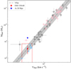 |
Fig. 7. BTFR for the sample of galaxies with redshift-independent distances from SPARC (gray+blue points; Lelli et al. 2016, 2019) supplemented with galaxies from Ponomareva et al. (2016, 2018, red points). The dashed line indicates the relation fitted for Vflat, with the shaded gray area representing the observed vertical scatter. The stars indicate ESO 358-60 on the relation for the best-fit model (red) and at a distance of 20 ± 1 Mpc (blue). The red box is determined by its top-right corner, where ESO 358-60 is positioned on the relation when using the upper limit derived from the rising RC model. |
To derive a distance from this baryonic mass we needed the stellar and gas mass individually. Using the total flux from the H I integrated intensity map (Fig. 2, left panel) and a flux measurement from 3.6 μm observations with the Infrared Array Camera (IRAC) on board the Spitzer satellite (Table 1; Bouquin et al. 2018), we calculated the distance to the galaxy as
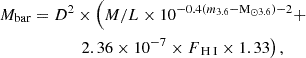 (1)
(1)
with D the distance in pc, Mbar the baryonic mass in M⊙, M/L the mass to light ratio for the 3.6 μm IRAC band 1, m3.6 and M⊙3.6 the galaxy’s apparent magnitude and the Sun’s absolute magnitude in the same band, respectively, and FH I the H I flux in Jy km s−1. Following Lelli et al. (2019), we used a factor of 1.33 to account for the presence of helium and used M/L = 0.5 for the mass-to-light ratio in the infrared. Finally, as our m3.6 is in the AB-magnitude system, we used M⊙3.6 = 6.08 (Willmer 2018). In this calculation we ignored the contribution of molecular hydrogen because Zabel et al. (2019) merely found upper limits for the galaxy and because the BTFR we used was derived under the same assumption.
The distances obtained for the various models are listed in Table 4. This table also shows the distance expected from the systemic velocity were the galaxy on the Hubble Flow and from the Cosmicflows-3 calculator (Kourkchi et al. 2020). It is obvious from these numbers that the BTFR distances are consistent with these independent distance estimates. To determine whether ESO 358-60 could be a likely member of the Fornax cluster at these distances, we estimated a lower boundary of the cluster by taking the minimal estimated distance (Dmin = 20 − 1.7 Mpc = 18.3 Mpc; Blakeslee et al. 2009) and subtracted twice the virial radius (Rvir = 0.7 Mpc; Drinkwater et al. 2001) from it. This leads to a lower boundary for the Fornax cluster of 16.9 Mpc and we see that all the BTFR distances fall significantly short of this distance. Only our upper distance limit, where the RC is forced to keep on rising, is consistent with the galaxy being part of Fornax at the upper ranges of the error bar.
ESO 358-60 distances as derived from the fitted RC by estimating its baryonic mass through the BTFR.
To ensure the applicability of the published BTFR to our galaxy, we compared several of its properties to a subsample of the SPARC galaxies that have similar Vflat. These galaxies are highlighted in blue in Fig. 7 and are defined by the box that can be drawn around ESO 358-60 by setting the top right corner as the location where the rising RC model falls on the BTFR (i.e., the red box in Fig. 7). We refer to these galaxies as the SPARC subsample in what follows.
Figure 8 compares the RCs of the SPARC subsample (gray lines) to ESO 358-60 at the best-fit distance (red and blue lines indicating the receding and approaching sides, respectively) and the same at the distance of Fornax (pink and light blue lines). It is obvious from this comparison that to be at the distance of Fornax, the RC of ESO 358-60 would have to be extremely slowly rising, that is to say, ESO 358-60 would have a very shallow matter distribution in the inner parts. Even the distance of 9.4 Mpc appears on the high side in this comparison as the best-fit RC rises more slowly than any of the curves in the SPARC subsample. The steepness of a RC, however, is also determined by the central distribution of mass (Garrido et al. 2005; Lelli 2022). The central surface brightness of ESO 358-60 (μ3.6 = 23.5 mag arcsec−2; Bouquin et al. 2018) falls on the lower end of the distribution compared to the other galaxies in Fig. 8 (SPARC-sub μ3.6 = 23.7–21.0 mag arcsec−2; Lelli et al. 2016). Hence, we would expect ESO 358-60 to have a RC that is rising relatively slowly compared to the SPARC subsample.
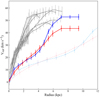 |
Fig. 8. RCs (gray lines) of the SPARC database in the neighborhood of ESO 358-60 on the TF relation. These galaxies are marked with light blue points in Fig. 7. Blue and red lines indicate the approaching and receding sides of the best-fit RC of ESO 358-60 at the BTFR-calculated distance. Light blue and pink lines show the same but at a distance of 20 Mpc. These lines continue outside the plotted area. |
The stellar mass of the galaxy at 9.4 ± 2.5 Mpc, as derived from the 3.6 μm flux, is 3 ± 2 × 10⁷ M⊙ and the H I mass is 3 ± 1 × 10⁸ M⊙. The significant errors on these masses come predominantly from the uncertainty on the distance. The stellar and H I masses of the SPARC subsample range from 0.6–17.6 × 10⁷ M⊙ and 0.5–4.1 × 10⁸ M⊙, respectively. This places the stellar mass of ESO 358-60 on the low end of SPARC subsample at the best-fit BTFR distance but at the high end at the distance of Fornax (Mstar Fornax = 12.3 × 10⁷ M⊙). The H I mass at the best-fit distance on the other hand corresponds to the mean H I mass in the SPARC subsample whereas it would be twice the maximum H I mass in this sample if ESO 358-60 were at the distance of Fornax (MH I Fornax = 11.5 × 10⁸). As the stellar and H I mass scale in the same way with distance the galaxy certainly has a high MH I/Mstar ratio of 9.6. For the SPARC subsample this ratio ranges from 0.5–13.0. For ESO 358-60 Su et al. (2021) find a stellar mass, rescaled to 9.4 Mpc, of 1.3 × 10⁷ from the g′, r′, i′ colors in the FDS. As this is even lower than the mass we derived from the 3.6 μm flux, we are convinced that the galaxy truly has a small stellar component.
To further investigate whether ESO 358-60 appears more as a field dwarf than a Fornax dwarf, we compared the g′−r′ color of ESO 358-60 to the colors of dwarfs in the Fornax cluster (Venhola et al. 2018) and in the field as found in the Canes Venatici region (Kovač 2007; Kovač et al. 2009). Figure 9 shows a color-magnitude diagram of the two samples and ESO 358-60 at the best-fit distance and at the distance of Fornax. Compared to the Fornax dwarfs ESO 358-60 is an outlier due to its blue colors, but compared to the dwarfs in the Canes Venatici region its color falls within the scatter of these galaxies. This is true regardless of which distance is considered.
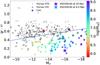 |
Fig. 9. Color-magnitude diagram of the dwarfs in the central 2.5 × 4 deg2 of the Fornax cluster (crosses indicate early-type dwarfs and circles late-type dwarfs) and those in the Canes Venatici region (squares). For the Fornax cluster, colored and black symbols are dwarfs detected and undetected in H I, respectively. The star symbols indicate ESO 358-60 at the best-fit distance (blue) and at 20 Mpc (purple). This figure is an updated version of Fig. 4. from Kleiner et al. (2023), with the Canes Venatici sample added and ESO 358-60 highlighted. |
In our literature search on the galaxy we found one more redshift-independent distance to ESO 358-60. The galaxy was included into the Cosmicflows-2 survey (Tully et al. 2013) who place the galaxy at 15.7 ± 3.1 Mpc based on an I-band TF-relation. The analysis presented in this paper provides several improvements on the Cosmicflows survey when considering individual galaxies. The most important of these improvements is that we included the H I mass in the relation, that is, we used the BTFR and not simply the TF relation. The BTFR provides a tighter relation, especially for low mass galaxies (McGaugh et al. 2000; Schombert et al. 2020) where the gas mass is as or more significant than the stellar mass. For such galaxies a relation based merely on optical light/stellar mass will overestimate the stellar contribution and thus yield a higher distance. This problem is exacerbated by the fact that Tully et al. (2013) have predominantly calibrated their relation on more massive galaxies (see their Fig. 8). In ESO 358-60 the H I mass is ∼10 times the stellar mass, and indeed if we repeat our analysis for Vflat and stellar masses instead of baryonic masses we find a distance of 13.7 ± 4.9 Mpc. Our distance is further confirmed by the Cosmicflows-3 calculator (Kourkchi et al. 2020) whose calculated distance corresponds to our distance at the location and systemic velocity of ESO 358-60. As such, we think no further explanation is required to account for the ∼6 Mpc difference with the Tully et al. (2013) result.
At the best-fit distance of 9.4 Mpc the galaxy would be closer to us compared to what we would expect from its systemic velocity assuming a Hubble flow. The difference implies a peculiar velocity toward the Fornax cluster ∼100 km s−1, indicating that the galaxy might feel the pull from the cluster and might eventually fall into it. If our best-fit distance is still overestimating the distance to ESO 358-60 the implied speed toward the cluster would increase simultaneously with its distance from the cluster. If this peculiar velocity is due to the gravitational attraction of the Fornax overdensity this would make it unlikely to be at a significantly lower distance.
From the BTFR we deduce a distance to ESO 358-60 of 9.4 ± 2.5 Mpc, placing it well in the foreground of the Fornax cluster. Such a distance fits not only better with Vflat but also with the overall RCs and H I content of low mass galaxies and the fact that the galaxy appears undisturbed and reasonably symmetric.
5. Radial motions
Radial motions, also known as streaming motions, are likely to be a crucial element in the overall evolution of spiral galaxies. Inflows to the centers of galaxies can feed the central massive black hole (Vollmer et al. 2008; Combes 2023), explain metallicity gradients (Lacey & Fall 1985; Sharda et al. 2021) and can in some cases even lead to bar-driven spiral arms (Sanders & Huntley 1976; Sellwood & Masters 2022). Foremost, inflows onto the inner disk are considered as an important candidate to sustain star formation in spiral galaxies (Ho et al. 2019; Wang & Lilly 2022). As there is not enough neutral gas available in the intergalactic medium to feed the H I in the inner disk directly from cosmological accretion (Kamphuis et al. 2022), such inflows might be required to transport gas from the outer disk to the star-forming disk.
Mechanisms resulting in large-scale radial outflows have theoretically received less interest despite the fact that they have been unambiguously detected in several galaxies (Schmidt et al. 2016). Outflows due to supernova explosions are expected to occur with a preferred vertical direction (Shapiro & Field 1976; Bregman 1980; Norman & Ikeuchi 1989) due to the steeper vertical density gradient. Indeed when holes, associated with supernova explosions, have been observed in H I the ordered combined flow is in the vertical direction (Boomsma et al. 2008) but the radial motions are circularly arranged around the center of the hole (Kamphuis et al. 1991) creating random motions on the scale of the galaxy. Small-scale radial outflows, as well as inflows, will occur along the spiral arms in disk galaxies (Kalnajs 1973) but we failed to find a theoretical background for larger scale outflows in the literature.
One can imagine that the tidal torques of an interaction or the deposition of a large quantity of high angular momentum gas in the inner disk can drive a large-scale outflow. Furthermore, additional pressure from a developing magnetic field driven by a magnetized turbulent dynamo (Beck et al. 2012) can lead to an outward pressure on the gas. However, this depends fully on the details of the emerging magnetic fields and gas distribution in the galaxy (Elstner et al. 2014). Such mechanisms need further investigation, which is beyond the scope of this paper, in order to detail their net effects on the gas kinematics. Overall, however, there is enough evidence pointing to radial gas flows as an integral part of the evolution of spiral galaxies.
Typically, observed radial motions in H I are on the order of a few km s−1 (Wong et al. 2004; Schmidt et al. 2016; Di Teodoro & Peek 2021) but can reach velocities of a few tens of km s−1 (Fraternali et al. 2002). When fitted with 2D tilted ring methods the determined radial motions are highly dependent on the underlying orientation of the model (Schmidt et al. 2016) and they are partially degenerate with the PA (Spekkens & Sellwood 2007; Wang & Lilly 2023; Sylos Labini et al. 2023). As such, they are typically difficult to identify, especially in the outer disk.
ESO 358-60 shows very clear radial motions in the center of the galaxy. They are undeniably present in the velocity field (Fig. 2) and also the 3D model is significantly improved by including radial motions (Fig. 5). The motions appear to be mostly confined inside the high density gas accompanying the high density disk. The largest radius where we detect radial motions is slightly beyond DH I (see Fig. 5). The amplitude of the motions in the model peaks at ∼15 km s−1 at a radius slightly below 100″. The motions then continue all the way inward to the center at an approximately constant level around 10 km s−1.
These motions imply a peak mass flow rate, calculated by multiplying the H I mass in a ring by its radial speed, of 0.5 M⊙ yr−1 at R = ∼100″. When we compare this to the star formation rate (SFR = 0.007 M⊙ yr−1; see Table 1), we see that such a flow would be adding more than enough gas to the inner disk to sustain the SFR if the flow were inward. Unfortunately, without further observations or modeling we cannot establish the direction of the radial motions. To establish the direction of the radial motions we need to know the near and far side of the galaxy, or in other words we need to know the direction of rotation. Often, this can be established from auxiliary data through the presence of the dust lane or the winding of the spiral arms but ESO 358-60 lacks visible spiral arms or a prominent dust lane. As such, currently we see no obvious path for determining, or even assuming, an orientation or rotational direction of the galaxy. Hence, we leave the interpretation of the radial motions in ESO 358-60 for a future publication.
6. Summary and conclusions
Due to a lack of anomalous gas in its surroundings and its very regular neutral hydrogen disk, the galaxy ESO 358-60 stands out from other H I detections in the MFS (Fig. 4; Serra et al. 2023). This motivated us to create a detailed model of the H I distribution in the galaxy to parametrize its disk in order to understand its regularity. By fitting a TRM in 3D to the H I data of the MFS, we were able to extract the kinematic and spatial parameters and obtain a detailed picture of the H I distribution in the galaxy. The H I distribution has a significant, but still almost symmetric, line-of-sight warp that starts around D25 and has a maximum shift of Δi ∼ 20°. Furthermore, radial motions are seen all over the observed optical disk, and these peak between D25 and DH I. The TRM further confirms the regularity of the disk.
The most straightforward explanation for the regularity of the H I disk, compared to other H I detections in the MFS, is a lack of interaction with Fornax’s ICM. From our TRM we establish a rotational velocity for ESO 358-60 of Vflat = 48.1 ± 1.4 km s−1. This translates to a redshift-independent distance of 9.4 ± 2.5 Mpc for ESO 358-60 when using this rotational velocity to place the galaxy on the BTFR as derived from the Vflat (McGaugh et al. 2000; Lelli et al. 2019). Comparing other properties of the galaxy, such as its H I mass or central stellar surface brightness, to those of galaxies from the SPARC database (Lelli et al. 2016, 2019) with similar Vflat led us to the conclusion that, at our derived distance, ESO 358-60 is a normal dwarf irregular with a stellar mass and central surface brightness at the low end of the distribution. Had the galaxy been at 20 Mpc, the distance of Fornax, it would have to have an extraordinary amount of H I compared to other galaxies with similar Vflat in the SPARC sample. The optical color of the galaxy matches field galaxies better than the other dwarfs found in Fornax. However, this is true regardless of the distance to ESO 358-60.
We conclude that ESO 358-60 at the retrieved redshift-independent distance is more than ∼10 Mpc in front of the Fornax cluster. As such, it is a field irregular galaxy that, at most, is starting to feel the gravitational attraction of the Fornax cluster. Our modeling shows that the observed H I distribution of the galaxy is best explained with a significant line-of-sight warp and radial motions in its inner disk, whose origins remain elusive for now.
We used a sech2 distribution in the model, which means the FWHM is ∼1.7627 × z0 = 0.7 kpc.
We used W20 as W50 is not available in SPARC. Wm50 is available in SPARC but it is based on the mean flux of the profile not the peak flux.
Acknowledgments
We thank Prof. J. English for developing a perceptually correct velocity field color map for a white background. We thank F. Loi for useful advice and discussions on the ICM density of the Fornax cluster. We would also like to thank two anonymous referees who helped to improve the paper through their careful reading and useful comments. The work at RUB is partially supported by the BMBF project 05A23PC1 for D-MeerKAT. The MeerKAT telescope is operated by the South African Radio Astronomy Observatory, which is a facility of the National Research Foundation, an agency of the Department of Science and Innovation. We acknowledge the use of the Ilifu cloud computing facility – www.ilifu.ac.za, a partnership between the University of Cape Town, the University of the Western Cape, the University of Stellenbosch, Sol Plaatje University, the Cape Peninsula University of Technology and the South African Radio Astronomy Observatory. The Ilifu facility is supported by contributions from the Inter-University Institute for Data Intensive Astronomy (IDIA – a partnership between the University of Cape Town, the University of Pretoria and the University of the Western Cape), the Computational Biology division at UCT and the Data Intensive Research Initiative of South Africa (DIRISA). This project has received funding from the European Research Council (ERC) under the European Union’s Horizon 2020 research and innovation programme (grant agreement no. 679627, “FORNAX”; and grant agreement no. 882793, “MeerGas”). The data of the MeerKAT Fornax Survey are reduced using the CARACal pipeline, partially supported by ERC Starting grant number 679627, MAECI (Italian Ministry of Foreign Affairs and International Cooperation) Grant Numbers PGR ZA23GR03 (RADIOMAP) and PGR ZA18GR02 (RADIOSKY2020), DSTNRF Grant Number 113121 as part of the ISARP Joint Research Scheme, and BMBF project 05A17PC2 for D-MeerKAT. Information about CARACal can be obtained online under the URL: https://caracal.readthedocs.io. This research has made use of the NASA/IPAC Extragalactic Database (NED), which is funded by the National Aeronautics and Space Administration and operated by the California Institute of Technology. This research has made use of the VizieR catalogue access tool, CDS, Strasbourg, France (DOI : 10.26093/cds/vizier). The original description of the VizieR service was published in 2000, A&AS 143, 23
References
- Beck, A. M., Lesch, H., Dolag, K., et al. 2012, MNRAS, 422, 2152 [NASA ADS] [CrossRef] [Google Scholar]
- Binggeli, B., Sandage, A., & Tarenghi, M. 1984, AJ, 89, 64 [NASA ADS] [CrossRef] [Google Scholar]
- Binggeli, B., Sandage, A., & Tammann, G. A. 1985, AJ, 90, 1681 [Google Scholar]
- Blakeslee, J. P., Jordán, A., Mei, S., et al. 2009, ApJ, 694, 556 [Google Scholar]
- Boomsma, R., Oosterloo, T. A., Fraternali, F., van der Hulst, J. M., & Sancisi, R. 2008, A&A, 490, 555 [NASA ADS] [CrossRef] [EDP Sciences] [Google Scholar]
- Bouquin, A. Y. K., Gil de Paz, A., Muñoz-Mateos, J. C., et al. 2018, ApJS, 234, 18 [NASA ADS] [CrossRef] [Google Scholar]
- Bradford, J. D., Geha, M. C., & van den Bosch, F. C. 2016, ApJ, 832, 11 [NASA ADS] [CrossRef] [Google Scholar]
- Bregman, J. N. 1980, ApJ, 236, 577 [NASA ADS] [CrossRef] [Google Scholar]
- Broeils, A. H., & Rhee, M. H. 1997, A&A, 324, 877 [NASA ADS] [Google Scholar]
- Chen, Y., Reiprich, T. H., Böhringer, H., Ikebe, Y., & Zhang, Y. Y. 2007, A&A, 466, 805 [NASA ADS] [CrossRef] [EDP Sciences] [Google Scholar]
- Chung, A., van Gorkom, J. H., Kenney, J. D. P., Crowl, H., & Vollmer, B. 2009, AJ, 138, 1741 [Google Scholar]
- Combes, F. 2023, Galaxies, 11, 120 [NASA ADS] [CrossRef] [Google Scholar]
- de Vaucouleurs, G., de Vaucouleurs, A., Corwin, H. G. Jr., et al. 1991, Third Reference Catalogue of Bright Galaxies (New York, NY: Springer) [Google Scholar]
- Deg, N., Palleske, R., Spekkens, K., et al. 2024, MNRAS, 525, 4663 [Google Scholar]
- Di Teodoro, E. M., & Peek, J. E. G. 2021, ApJ, 923, 220 [NASA ADS] [CrossRef] [Google Scholar]
- Dressler, A. 1980, ApJS, 42, 565 [NASA ADS] [CrossRef] [Google Scholar]
- Drinkwater, M. J., Gregg, M. D., & Colless, M. 2001, ApJ, 548, L139 [Google Scholar]
- Elstner, D., Beck, R., & Gressel, O. 2014, A&A, 568, A104 [NASA ADS] [CrossRef] [EDP Sciences] [Google Scholar]
- Ferguson, H. C. 1989, AJ, 98, 367 [Google Scholar]
- Fraternali, F., van Moorsel, G., Sancisi, R., & Oosterloo, T. 2002, AJ, 123, 3124 [CrossRef] [Google Scholar]
- Garrido, O., Marcelin, M., Amram, P., et al. 2005, MNRAS, 362, 127 [NASA ADS] [CrossRef] [Google Scholar]
- Gunn, J. E., & Gott, J. R. III 1972, ApJ, 176, 1 [NASA ADS] [CrossRef] [Google Scholar]
- Ho, S. H., Martin, C. L., & Turner, M. L. 2019, ApJ, 875, 54 [NASA ADS] [CrossRef] [Google Scholar]
- Iodice, E., Capaccioli, M., Grado, A., et al. 2016, ApJ, 820, 42 [Google Scholar]
- Józsa, G. I. G., Kenn, F., Klein, U., & Oosterloo, T. A. 2007, A&A, 468, 731 [NASA ADS] [CrossRef] [EDP Sciences] [Google Scholar]
- Kalnajs, A. J. 1973, PASA, 2, 174 [Google Scholar]
- Kamphuis, P. 2024, pyFAT: Python Fully Automated TiRiFiC, Astrophysics Source Code Library [record ascl:2407.002] [Google Scholar]
- Kamphuis, J., Sancisi, R., & van der Hulst, T. 1991, A&A, 244, L29 [Google Scholar]
- Kamphuis, P., Józsa, G. I. G., Oh, S. H., et al. 2015, MNRAS, 452, 3139 [NASA ADS] [CrossRef] [Google Scholar]
- Kamphuis, P., Jütte, E., Heald, G. H., et al. 2022, A&A, 668, A182 [NASA ADS] [CrossRef] [EDP Sciences] [Google Scholar]
- Kleiner, D., Serra, P., Maccagni, F. M., et al. 2023, A&A, 675, A108 [NASA ADS] [CrossRef] [EDP Sciences] [Google Scholar]
- Kourkchi, E., Courtois, H. M., Graziani, R., et al. 2020, AJ, 159, 67 [NASA ADS] [CrossRef] [Google Scholar]
- Kovač, K. 2007, Ph.D. Thesis, University of Groningen, The Netherlands [Google Scholar]
- Kovač, K., Oosterloo, T. A., & van der Hulst, J. M. 2009, MNRAS, 400, 743 [CrossRef] [Google Scholar]
- Lacey, C. G., & Fall, S. M. 1985, ApJ, 290, 154 [NASA ADS] [CrossRef] [Google Scholar]
- Lelli, F. 2022, Nat. Astron., 6, 35 [NASA ADS] [CrossRef] [Google Scholar]
- Lelli, F., McGaugh, S. S., & Schombert, J. M. 2016, AJ, 152, 157 [Google Scholar]
- Lelli, F., McGaugh, S. S., Schombert, J. M., Desmond, H., & Katz, H. 2019, MNRAS, 484, 3267 [NASA ADS] [CrossRef] [Google Scholar]
- Leroy, A. K., Sandstrom, K. M., Lang, D., et al. 2019, ApJS, 244, 24 [Google Scholar]
- Loni, A., Serra, P., Sarzi, M., et al. 2023, MNRAS, 523, 1140 [CrossRef] [Google Scholar]
- Maddox, N., Serra, P., Venhola, A., et al. 2019, MNRAS, 490, 1666 [Google Scholar]
- Matthews, L. D., & Gallagher, J. S. I. 1997, AJ, 114, 1899 [NASA ADS] [CrossRef] [Google Scholar]
- McGaugh, S. S., Schombert, J. M., Bothun, G. D., & de Blok, W. J. G. 2000, ApJ, 533, L99 [Google Scholar]
- Norman, C. A., & Ikeuchi, S. 1989, ApJ, 345, 372 [Google Scholar]
- O’Brien, J. C., Freeman, K. C., & van der Kruit, P. C. 2010, A&A, 515, A62 [CrossRef] [EDP Sciences] [Google Scholar]
- Ponomareva, A. A., Verheijen, M. A. W., & Bosma, A. 2016, MNRAS, 463, 4052 [NASA ADS] [CrossRef] [Google Scholar]
- Ponomareva, A. A., Verheijen, M. A. W., Papastergis, E., Bosma, A., & Peletier, R. F. 2018, MNRAS, 474, 4366 [Google Scholar]
- Sanders, R. H., & Huntley, J. M. 1976, ApJ, 209, 53 [Google Scholar]
- Schmidt, T. M., Bigiel, F., Klessen, R. S., & de Blok, W. J. G. 2016, MNRAS, 457, 2642 [NASA ADS] [CrossRef] [Google Scholar]
- Schombert, J., McGaugh, S., & Lelli, F. 2020, AJ, 160, 71 [NASA ADS] [CrossRef] [Google Scholar]
- Schröder, A., Drinkwater, M. J., & Richter, O. G. 2001, A&A, 376, 98 [NASA ADS] [CrossRef] [EDP Sciences] [Google Scholar]
- Sellwood, J. A., & Masters, K. L. 2022, ARA&A, 60, 36 [Google Scholar]
- Serra, P., Maccagni, F. M., Kleiner, D., et al. 2023, A&A, 673, A146 [NASA ADS] [CrossRef] [EDP Sciences] [Google Scholar]
- Shapiro, P. R., & Field, G. B. 1976, ApJ, 205, 762 [NASA ADS] [CrossRef] [Google Scholar]
- Sharda, P., Krumholz, M. R., Wisnioski, E., et al. 2021, MNRAS, 504, 53 [NASA ADS] [CrossRef] [Google Scholar]
- Spekkens, K., & Sellwood, J. A. 2007, ApJ, 664, 204 [NASA ADS] [CrossRef] [Google Scholar]
- Steer, I., Madore, B. F., Mazzarella, J. M., et al. 2017, AJ, 153, 37 [Google Scholar]
- Su, A. H., Salo, H., Janz, J., et al. 2021, A&A, 647, A100 [EDP Sciences] [Google Scholar]
- Sylos Labini, F., Straccamore, M., De Marzo, G., & Comerón, S. 2023, MNRAS, 524, 1560 [Google Scholar]
- Tully, R. B., & Fisher, J. R. 1977, A&A, 54, 661 [NASA ADS] [Google Scholar]
- Tully, R. B., Courtois, H. M., Dolphin, A. E., et al. 2013, AJ, 146, 86 [NASA ADS] [CrossRef] [Google Scholar]
- Venhola, A., Peletier, R., Laurikainen, E., et al. 2018, A&A, 620, A165 [NASA ADS] [CrossRef] [EDP Sciences] [Google Scholar]
- Vollmer, B., Beckert, T., & Davies, R. I. 2008, A&A, 491, 441 [NASA ADS] [CrossRef] [EDP Sciences] [Google Scholar]
- Wang, E., & Lilly, S. J. 2022, ApJ, 927, 217 [NASA ADS] [CrossRef] [Google Scholar]
- Wang, E., & Lilly, S. J. 2023, ApJ, 944, 143 [NASA ADS] [CrossRef] [Google Scholar]
- Willmer, C. N. A. 2018, ApJS, 236, 47 [Google Scholar]
- Wong, T., Blitz, L., & Bosma, A. 2004, ApJ, 605, 183 [NASA ADS] [CrossRef] [Google Scholar]
- Zabel, N., Davis, T. A., Smith, M. W. L., et al. 2019, MNRAS, 483, 2251 [Google Scholar]
All Tables
ESO 358-60 distances as derived from the fitted RC by estimating its baryonic mass through the BTFR.
All Figures
|
Fig. 1. Left: g-band optical image from the Fornax Deep Survey (FDS; Iodice et al. 2016; Venhola et al. 2018) overlaid with intensity contours of the H I (see Fig. 2). Right: Far-ultraviolet image from GALEX observations overlaid with velocity contours extracted from the 21 cm observations (Fig. 2). The blue circle marks what appears to be a large star-forming region. |
| In the text | |
|
Fig. 2. Moment maps of the H I in the galaxy ESO 358-60. Dark gray contours show the data. The blue contours indicate the automatic model (in the top panels) and the best-fit model (in the bottom panels). Left: Moment 0 or integrated intensity map of the galaxy. Contours are at |
| In the text | |
|
Fig. 3. Global line profile of ESO 358-60. The black line indicates the data, the blue the best-fit model, and the gray the automatic model. The vertical dashed red line indicates the systemic velocity, and the horizontal line the uncorrected W20. |
| In the text | |
|
Fig. 4. g′-band image of the 2 deg2 surrounding ESO 358-60 from the FDS (Iodice et al. 2016; Venhola et al. 2018) overlaid with the lowest reliable contours (3σ) of the 98″ and 41″ resolutions of the MFS. For the 21″ resolution, we plot the contour corresponding to ∼1 M⊙ pc−2. The beams are displayed in the bottom-left corner. All galaxies that are spectroscopically confirmed in the field are labeled, and the background color of the label indicates the systemic velocity of the system. The color bar on the right shows the correspondence between color and velocity. Galaxies identified in the FDS, but not spectroscopically confirmed, are marked with a red x. |
| In the text | |
|
Fig. 5. Fitted parameters for the various models. Light gray lines represent the PYFAT model, black lines the single disk model, and the blue (approaching) and red (receding) lines the final best-fit model. The panels show the rotation velocities (a), surface brightness distribution (b), inclination (c), PA (d), and radial motions (e), all as function of radius. The vertical dot-dashed gray line indicates R25, and the vertical dashed lines in panel b mark where the surface brightness is equal to 1 M⊙ pc−2. |
| In the text | |
|
Fig. 6. PV diagram along the major axis. Gray contours and the color scale show the data, and blue contours show the best-fit model. Contours are at 1.5, 3, 6, 12, 24 × σ with σ = 0.24 mJy beam−1 (3.2 × 1018 cm−2 in a channel). The dashed gray line indicates the spatial fitted center, and the dashed colored line indicates the fitted systemic velocity of the best-fit model. The blue circles indicate the Vobs = Vrot × sin(i) of the best-fit model, and the white circles the same for the rising model (see text). To be concurrent with the right ascension, offsets are decreasing from left to right. |
| In the text | |
|
Fig. 7. BTFR for the sample of galaxies with redshift-independent distances from SPARC (gray+blue points; Lelli et al. 2016, 2019) supplemented with galaxies from Ponomareva et al. (2016, 2018, red points). The dashed line indicates the relation fitted for Vflat, with the shaded gray area representing the observed vertical scatter. The stars indicate ESO 358-60 on the relation for the best-fit model (red) and at a distance of 20 ± 1 Mpc (blue). The red box is determined by its top-right corner, where ESO 358-60 is positioned on the relation when using the upper limit derived from the rising RC model. |
| In the text | |
|
Fig. 8. RCs (gray lines) of the SPARC database in the neighborhood of ESO 358-60 on the TF relation. These galaxies are marked with light blue points in Fig. 7. Blue and red lines indicate the approaching and receding sides of the best-fit RC of ESO 358-60 at the BTFR-calculated distance. Light blue and pink lines show the same but at a distance of 20 Mpc. These lines continue outside the plotted area. |
| In the text | |
|
Fig. 9. Color-magnitude diagram of the dwarfs in the central 2.5 × 4 deg2 of the Fornax cluster (crosses indicate early-type dwarfs and circles late-type dwarfs) and those in the Canes Venatici region (squares). For the Fornax cluster, colored and black symbols are dwarfs detected and undetected in H I, respectively. The star symbols indicate ESO 358-60 at the best-fit distance (blue) and at 20 Mpc (purple). This figure is an updated version of Fig. 4. from Kleiner et al. (2023), with the Canes Venatici sample added and ESO 358-60 highlighted. |
| In the text | |
Current usage metrics show cumulative count of Article Views (full-text article views including HTML views, PDF and ePub downloads, according to the available data) and Abstracts Views on Vision4Press platform.
Data correspond to usage on the plateform after 2015. The current usage metrics is available 48-96 hours after online publication and is updated daily on week days.
Initial download of the metrics may take a while.