| Issue |
A&A
Volume 695, March 2025
|
|
|---|---|---|
| Article Number | A104 | |
| Number of page(s) | 23 | |
| Section | Catalogs and data | |
| DOI | https://doi.org/10.1051/0004-6361/202453167 | |
| Published online | 14 March 2025 | |
Mapping Hα excess candidate point sources in the southern hemisphere using S-PLUS data
1
Instituto de Astrofísica de La Plata (CCT La Plata – CONICET – UNLP),
B1900FWA,
La Plata, Argentina
2
Departamento de Astronomia, Instituto de Astronomia, Geofísica e Ciências Atmosféricas da USP, Cidade Universitária,
05508-900
São Paulo, SP, Brazil
3
Departamento de Física, Universidade Federal de Sergipe,
Av. Marechal Rondon S/N,
49100-000
São Cristóvão, SE, Brazil
4
Observatório Nacional,
Rua Gal. José Cristino 77,
20921-400
Rio de Janeiro, RJ, Brazil
5
Institute for Astronomy, Astrophysics, Space Applications and Remote Sensing, National Observatory of Athens,
GR 15236
Penteli, Greece
6
Universidade Federal do Rio de Janeiro, Observatório do Valongo,
Ladeira do Pedro Antônio, 43, Saúde CEP
20080-090
Rio de Janeiro, RJ, Brazil
7
Instituto de Astrofísica de Andalucía, CSIC,
Apt 3004,
18080
Granada, Spain
8
Instituto de Física Aplicada a las Ciencias y las Tecnologías, Universidad de Alicante, San Vicent del Raspeig,
03080
Alicante, Spain
9
Instituto de Astronomía y Ciencias Planetarias, Universidad de Atacama,
Copayapu 485,
Copiapó, Chile
10
Millennium Institute of Astrophysics,
Nuncio Monseñor Sotero Sanz 100, Of. 104,
Providencia, Santiago, Chile
11
Departmento de Astronomía, Universidad de La Serena,
Avenida Raúl Bitrán 1305,
La Serena, Chile
12
International Gemini Observatory/NSF NOIRLab,
Casilla 603,
La Serena, Chile
13
Departamento de Física, Universidade Federal de Santa Catarina,
Florianópolis, SC
88040-900,
Brazil
14
Rubin Observatory Project Office,
950 N. Cherry Ave.,
Tucson, AZ
85719,
USA
15
The Observatories of the Carnegie Institution for Science,
813 Santa Barbara St,
Pasadena,
CA
91101, USA
★ Corresponding author; This email address is being protected from spambots. You need JavaScript enabled to view it.
Received:
26
November
2024
Accepted:
26
January
2025
Abstract
Context. We use the Southern Photometric Local Universe Survey (S-PLUS) Fourth Data Release (DR4) to identify and classify Hα excess point source candidates in the southern sky. This approach combines photometric data from 12 S-PLUS filters with machine learning techniques to improve source classification and advance our understanding of Hα-related phenomena.
Aims. Our goal is to enhance the classification of Hα excess point sources by distinguishing between Galactic and extragalactic objects, particularly those with redshifted emission lines, and to identify sources where the Hα excess is associated with variability phenomena, such as short-period RR Lyrae stars.
Methods. We selected Hα excess candidates using the (r − J0660) versus (r − i) colour–colour diagram from the S-PLUS main survey (MS) and Galactic Disk Survey (GDS). For the MS sample, dimensionality reduction was achieved using UMAP, followed by HDBSCAN clustering. We refined this by incorporating infrared data, which improved the separation of source types. A random forest model was then trained on the clustering results to identify key colour features for the classification of Hα excess sources. New effective colour–colour diagrams were constructed by combining data from S-PLUS MS and infrared data. These diagrams, alongside tentative colour criteria, offer a preliminary classification of Hα excess sources without the need for complex algorithms.
Results. Combining multi-wavelength photometric data with machine learning techniques significantly improved the classification of Hα excess sources. We identified 6956 sources with an excess in the J0660 filter, and cross-matching with SIMBAD allowed us to explore the types of objects present in our catalogue, including emission-line stars, young stellar objects, nebulae, stellar binaries, cataclysmic variables, variable stars, and extragalactic sources such as Quasi-Stellar Objects (QSOs), Active Galactic Nuclei (AGN), and galaxies. The cross-match also revealed X-ray sources, transients, and other peculiar objects. Using S-PLUS colours and machine learning, we successfully separated RR Lyrae stars from other Galactic stars and from extragalactic objects. Additionally, we achieved a clear separation between Galactic and extragalactic sources. However, distinguishing cataclysmic variables from QSOs at specific redshifts remained challenging. Incorporating infrared data refined the classification, enabling us to separate Galactic from extragalactic sources and to distinguish cataclysmic variables from QSOs. The Random Forest model, trained on HDBSCAN results, highlighted key colour features that distinguish the different classes of Hα excess sources, providing a robust framework for future studies, such as follow-up spectroscopy.
Key words: techniques: photometric / surveys / novae, cataclysmic variables / quasars: emission lines
© The Authors 2025
 Open Access article, published by EDP Sciences, under the terms of the Creative Commons Attribution License (https://creativecommons.org/licenses/by/4.0), which permits unrestricted use, distribution, and reproduction in any medium, provided the original work is properly cited.
This article is published in open access under the Subscribe to Open model. This email address is being protected from spambots. You need JavaScript enabled to view it. to support open access publication.
1 Introduction
Hydrogen Balmer emission lines are primarily produced by radiative processes, particularly radiative excitation and ionization, which dominate over collisional excitation under typical nebular conditions. For example, the Einstein A-coefficient for the Hα transition (A32 ≈ 4.41 × 10⁷ s−1) is significantly larger than the typical collisional excitation rate coefficient (~10−9 to 10−8 cm3 s−1) at electron temperatures around 10 000 K. While collisional excitation can become more important in shock-heated or very dense environments, it generally remains secondary in the diffuse conditions of most nebulae. Because the Universe is abundant in hydrogen, the observation of these electronic transitions offers an important window into the study of astrophysical objects. Among all the possible electronic transitions, the Balmer series represents an extremely useful tool in astronomy because it falls in the commonly used optical spectral range. In particular, the Hα emission line, with a rest-frame vacuum wavelength of 6564.614 Å, corresponding to the electron transition from n = 3 to n = 2, is the strongest in both emission and absorption. It is the most widely used line for identifying various types of objects, such as star-forming regions, H II regions, planetary nebulae (PNe), supernovae, novae, young stellar objects (YSOs), Herbig-Haro objects, circumstellar disks, post-asymptotic and asymptotic giant stars (AGBs), red giant branch stars (RGBs), and active late-type dwarfs. Among massive stars, emission lines are observed in Be stars with decretion disks, B[e] supergiants, luminous blue variables (LBVs), Wolf-Rayet (WR) stars, and interacting binary systems that are experiencing mass exchange, such as symbiotic stars (SySts), cataclysmic variables (CVs), among others.
In high-redshift sources, such as starburst galaxies and quasistellar objects (QSOs), Hα emission is present, but redshifted to longer wavelengths. However, when we detect emission near 6563 Å from high-redshift sources, the recombination of Hα is not the cause; instead, it is the outcome of UV emission lines that have shifted towards the visible spectrum.
Most existing databases of the aforementioned classes of objects are not homogeneous and remain far from complete, even in the local universe. Some classes are highly populated, while others are significantly under-represented. For example, there are ∼300 known SySts in the Milky Way, but only 75 in nearby galaxies (Akras et al. 2019b; Merc et al. 2019), although new discoveries are being made every year (e.g. Merc et al. 2020; Akras et al. 2021; Merc et al. 2021, 2022; Munari et al. 2021, 2022; Akras 2023). The number of known PNe in our Galaxy is of the order of ∼3500 (Parker et al. 2016), which may represent only 15–30% of the total population (Frew 2008; Jacoby et al. 2010).
Hα surveys have been conducted with varying angular resolutions, sky coverage, and sensitivity. Some surveys, despite their modest spatial resolutions, have successfully resolved extended nebular emissions, enabling the study of supernova remnants, galaxy groups, and star-forming regions (e.g. Davies et al. 1976; Blair & Long 2004; Jaiswal & Omar 2016; Cook et al. 2019). Others, with higher spatial resolution, have revealed compact emission-line sources in the Milky Way and nearby galaxies. Examples of them are the INT Photometric Hα survey (IPHAS; Drew et al. 2005; Barentsen et al. 2014), the SuperCOSMOS Hα survey with the UK Schmidt Telescope (UKST) of the Anglo-Australian Observatory (Parker et al. 2005), and the VST Photometric Hα Survey (VPHAS+; Drew et al. 2014).
Colour–colour diagrams from photometric surveys are also used to identify possible Hα emitters. For example, the (r - Hα) versus (r – i) colour–colour diagram, and other similar diagrams, have been used to find CVs (Witham et al. 2006, 2007), YSOs (Vink et al. 2008), SySts (Corradi et al. 2008, 2011; Corradi & Giammanco 2010; Miszalski & Mikołajewska 2014; Mikołajewska et al. 2014, 2017; Akras et al. 2019c), early-type emission-line stars (Drew et al. 2008), and PNe (Miszalski et al. 2009; Viironen et al. 2009; Sabin et al. 2010; Akras et al. 2019a). Additionally, other combinations of broadband filters have been tailored to distinguish active galactic nuclei (AGN), QSOs, and compact PNe based on their distinct photometric signatures (Peters et al. 2015; Gutiérrez-Soto et al. 2024).
In particular, the class of Be stars is the most common, nearly 50%, in the total sample of Hα emitters in IPHAS with only a moderate r-Hα excess, strongly limited near-infrared colours (J – H, H – K; Corradi et al. 2008; Raddi et al. 2015, and moderate mid-infrared colours (e.g. W1 – W4, W3 – W4; Akras et al. 2019c). In addition to the identification of different classes of Hα emitters, the r–Hα excess derived from Hα photometric surveys such as the IPHAS and VPHAS+, it also provides a new automatic way to derive the accretion rate in large numbers of YSOs (Barentsen et al. 2011; Kalari et al. 2015).
Witham et al. (2008) developed a method for selecting Hα emission-line sources in the IPHAS survey by implementing the aforementioned colour–colour diagram (r–Hα) versus (r–i). Objects with an Hα excess line were identified by iteratively fitting the stellar locus and considering as candidates those objects that fall several sigma above this stellar locus in the r–Hα colour. This conservative method yields a total of 4853 point sources in the IPHAS catalogue that exhibit strong photometric evidence for Hα emission. They obtained spectra from around 300 sources, confirming more than 95 percent of them as genuine emission-line stars.
Monguió et al. (2020) developed the INT Galactic Plane Survey (IGAPS) by merging the IPHAS and the UV-excess Survey of the Northern Galactic Plane (UVEX; Groot et al. 2009) optical surveys. The IGAPS catalogue includes 295.4 million photometric measurements in the i, r, narrowband Hα, g, and URGO filters. It identifies 8292 candidate emission-line stars and over 53 000 variable stars with confidence greater than 5σ.
More recently, Fratta et al. (2021) introduced a technique using Gaia data to identify Hα-bright sources in the IPHAS catalogue. They partitioned the data based on Gaia colour-absolute magnitude and Galactic coordinates to minimize contamination, and then applied the strategy from Witham et al. (2008) to these partitions.
Two ongoing multi-band surveys are observing the sky in a systematic, complementary way, with five broadband and seven narrowband filters, including Hα: the Javalambre Photometric Local Universe Survey (J-PLUS1; Cenarro et al. 2019), covering the northern celestial hemisphere, and the Southern-Photometric Local Universe Survey (S-PLUS2; Mendes de Oliveira et al. 2019), covering the southern sky with a twin 83 cm telescope and filter system. The first survey is paving the way for an even more ambitious survey, the Javalambre Physics of the Accelerating Universe Astrophysical Survey (J-PAS; Benitez et al. 2014 and miniJ-PAS; Bonoli et al. 2021), which will observe the northern sky with 56 narrowband filters. As source hunters, the spectral energy distributions provided by these surveys enable an unprecedented source classification using photometry only. However, in the era of Big Data, efficient investigation tools are required to deal with their massive imaging and catalogue production, and machine learning techniques have been increasingly used to explore these datasets (e.g. Bom et al. 2021; Yang et al. 2022).
Here we present a census of Hα excess point-like sources from the S-PLUS DR4, identified using the (r – J0660) versus (r – i) colour–colour diagram. Advanced machine learning techniques are employed to improve the identification and classification of these sources from the S-PLUS DR4 dataset. Specifically, we use Uniform Manifold Approximation and Projection (UMAP; Becht et al. 2019; McInnes et al. 2020) for dimensionality reduction followed by Hierarchical Density-Based Spatial Clustering of Applications with Noise (HDBSCAN; Campello et al. 2013) clustering to group sources based on their multiwavelength photometric signatures. This approach allows us to handle high-dimensional data effectively and uncover patterns that traditional methods might overlook. Additionally, we incorporate Wide-Field Infrared Survey Explorer (WISE; Wright et al. 2010) data and apply a random forest (Breiman 2001) model to refine our classification and identify key features that distinguish different types of Hα excess sources.
Section 2 describes the observations related to the S-PLUS project, including important information on the fourth data release, photometry, and data handling. Section 3.3 presents the technique implemented to select the Hα-feature sources. Section 4 includes the analysis of the results. In Sect. 5, we present the machine learning methods used to analyse and make a more accurate classification of the Hα sources. Finally, in Sect. 6 we discuss our main results and present out conclusions.
2 S-PLUS Survey overview
S-PLUS surveys the southern sky using the 12 filters from the Javalambre filter system (Marín-Franch et al. 2012), a spanning the wavelength range from 3000 Å to 10 000 Å. This system comprises seven narrowband filters (J0378, J0395, J0410, J0430, J0515, J0660, J0861, and five broadband Sloan-like (Fukugita et al. 1996) filters (see Fig. 1). The narrowband J0660 filter used in S-PLUS is centred at λ 6614Å and has a width of ≈l47Å (Table 2 of Mendes de Oliveira et al. 2019). Consequently, it covers both the Hα and the [N II] doublet λλ 6548, 6584 spectral lines for sources up to a redshift of ≈0.02. S-PLUS is conducted using a dedicated 0.83 m robotic telescope located at Cerro Tololo, Chile (Mendes de Oliveira et al. 2019).
This work uses data from S-PLUS DR4 (Herpich et al. 2024). DR4 encompasses 171 fields at very low galactic latitudes (|b| < 15°), 341 new fields added to the Main Survey (MS) footprint (with |b| > 30°), in addition to the fields carried over from DR3, and 150 fields within the Magellanic Clouds region. This accumulation results in a total of 1629 fields in DR4, covering an expansive area of 3022.7 square degrees. Notably, this coverage includes 347.4 square degrees within the disk regions and 289.5 square degrees within the Magellanic Clouds Survey (MC). Here, we explore the MS and Galactic Disk Survey (GDS), we primary goal of identify objects with Hα excess in S-PLUS DR4.
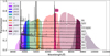 |
Fig. 1 Transmission curves of the S-PLUS filter set. The narrowband filter J0660 includes the Hα emission line. Overplotted are the spectra of different classes of emission-line objects. From top to bottom: a PN, a symbiotic star, an extragalactic H II region, a blue compact/H II galaxy, a YSO, a CV star, a B[e] star, a star-forming galaxy, and a QSO at a redshift of ~3.3l. |
2.1 Flux calibration
The flux calibration of the S-PLUS survey was performed using a combination of external and internal calibration steps to ensure uniformity and accuracy across the entire survey footprint. The calibration process begins with an external calibration, where synthetic photometry is integrated with a reference catalogue to derive the calibrated magnitudes for the different filters. Zero points (ZPs) are determined as the difference between the predicted magnitudes from the synthetic models and the instrumental magnitudes observed in the survey. The synthetic spectral library for this step was constructed by convolving the library of Coelho (2014) with the transmission curves of multiple reference catalogues and the S-PLUS filter system.
In regions where external calibration data are unavailable, such as for the u, J0410, and J0430 filters, a stellar locus method is applied. This technique calibrates these filters by leveraging the stellar locus, a relationship between specific filter magnitudes observed for a population of stars. This step is crucial when external reference data are insufficient. Once the external calibration is complete, an internal calibration step further refines the ZPs by using pre-calibrated narrowband filters, which better constrain the synthetic models and improve the calibration accuracy to 0.01–0.02 mag. This internal calibration is particularly valuable for cases where external calibration might be lacking or less precise.
Finally, the calibration is aligned to the Gaia system by applying an average offset derived from synthetic photometry, ensuring consistency across the entire survey region. This final alignment guarantees that the flux calibration is homogeneous and compatible with the Gaia photometric system, as outlined by Herpich et al. (2024).
2.2 Filter sequence and observational strategy
In the S-PLUS survey, the filters are observed in the following fixed sequence: u, J0378, J0395, J0410, J0430, J0515, g, r, i, z, J0660, J0861. Each field is observed for approximately 90 minutes, with three exposures taken per filter, accounting for readout times and filter transitions. This sequence enables the study of variability in sources over different timescales and wavelengths. Furthermore, the time gap between the r and J0660 filters, caused by the intervening filters, plays a crucial role in detecting variability in sources with periods that are captured within this observational sequence.
3 Selection procedure
The selection of Hα candidates is based on applying a series of restrictions to catalogues provided by S-PLUS DR4 in the r, i, and J0660 bands. We have reinforced this information in the Galactic disk region by generating catalogues with point spread function (PSF) photometry using SExtractor + PSFEx.
3.1 Main survey (MS) data
Amongst the different aperture photometry available in the S-PLUS DR4 catalogue, the PStotal3 photometry is used (Almeida-Fernandes et al. 2022). To acquire data with high- quality photometry and identify compact objects in the MS, several criteria were applied:
Objects must exhibit an r magnitude within the range of 13 < r ≤ 19.5.
J0660 magnitude <19.4 and i magnitude <19.2, which are average photometric depths for a S/N > 10 threshold (see Table 4 of Almeida-Fernandes et al. 2022).
Errors less than 0.2 mag in the r, J0660, and i filters.
The signal-to-noise ratio (S/N) in the respective filter should be higher than 10.
Objects should have SEX_FLAGS_DET < 4. The SEX_FLAGS_DET parameter is a bit-flag generated by SExtractor, indicating potential issues during photometry. The value corresponds to the sum of all flags, each represented by an integer. A value lower than four indicates that the flags can only sum up to: 0 (no flag), 1 (a minor issue: blending with another object), 2 (another minor issue: the object was originally blended with another one), or 3 (a combination of minor issues). Therefore, at most, we are selecting data affected by a combination of two minor issues, such as contamination from a nearby source and previous blending among sources. For more information, we refer to the documentation4.
Objects must satisfy CLASS_STAR_r = 1 and CLASS_STAR_i = 1, corresponding to the binary classification in the r and i filters, where a value of 1 indicates that the source is classified as a point source (star) in each filter, and a value of 0 denotes non-stellar or extended sources. The CLASS_STAR parameter in SExtractor represents a probability value ranging from 0 to 1, with higher values indicating a greater likelihood that the source is a point source. In our selection, we applied this binary classification for CLASS_STAR_r and CLASS_STAR_i to ensure a higher likelihood that the sources are stars.
Additional criteria were implemented. These criteria are systematically chosen to ensure the robustness and reliability of the selected sample, considering various photometric and morphological properties of the sources.
We consider the morphological properties of the sources by imposing a threshold on ellipticity. Sources with ellipticity values greater than 0.2 are likely to have non-galactic types (e.g. AGN, QSOs, galaxies, radio sources) or irregular shapes and are therefore excluded.
We select sources with compact morphology by constraining the radius enclosing 50% of the total flux, setting FLUX_RADIUS_50 < 3. Sources with a flux radius exceeding 3 pixels are likely to have extended morphology and are thus excluded from the sample.
These constraints led to the selection of 6 655 139 sources. The data were obtained by querying the project’s database using the splusdata Python package, accessible via S-PLUS Cloud5.
3.2 Galactic disk survey (GDS)
We used a combination of SExtractor6 (Bertin & Arnouts 1996) and PSFex7 (Bertin 2011) for source detection and posterior photometric measurements. We performed a serie of proofs with different SExtractor (e.g. DETECT_MINAREA, DETECT_THRESH, PHOT_APERTURES) and PSFex (e.g. PSF_SIZE, PHOTFLUX_KEY, PSFVAR_DEGREES) parameters plus test images (e.g. BACKGROUND, BACKGROUND_RMS, -BACKGROUND, APERTURES) to detect the largest number of objects with the best measurement possible of PSF-magnitude, MAG_PSF. The crucial parameters for PSF photometry are listed in Table A.1. The detection was performed on images from which their median-filtered versions was subtracted; faint sources are detected more easily in a median-subtracted image (González-Lópezlira et al. 2017). All median images were produced with a 11×11 pix2 median-filter.
The PSF photometry method is described in González Lópezlira et al. (2017), Lomelí-Núñez et al. (2022), González Lópezlira et al. (2022) and Lomelí-Núñez (in prep.). A brief description of the photometric method is given below. a) First run of SExtractor: we run SExtractor for the first time for the detection and selection of point sources based on their brightness versus compactness, as measured by the parameters of SExtractor MAG_AUTO (a Kron-like elliptical aperture magnitude; Kron 1980) and FLUX_RADIUS (similar to the effective radius). For the creation of the PSF, we selected sources in the space MAG_AUTO versus FLUX_RADIUS, in a range to: 12≲ MAG_AUTO ≲ 21.5 and 1 ≲ FLUX_RADIUS ≲ 3.5. Because we are observing towards the Galactic disk, the number of sources to creation each PSF can reach ~20 000 sources, which was not possible in the previous works because they were focused on extragalactic sources far away from the Galactic disk. b) PSF creation: we used PSFex to create the PSF using the point sources selected in the last step. The spatial variations of the PSF were modelled using third-degree polynomials as a function of the pixel coordinates (X, Y). For PSF creation, the flux of each star was measured in an aperture of 9 pixels of radius in all bands (equivalent to 4″.95×4″.95); this aperture, determined through the growth-curve method for each passband, is large enough to measure the total flux of the stars, but small enough to reduce the likelihood of contamination by external sources. c) Second run of SExtractor: we run SExtractor again this time using the PSF created in the last step as an input parameter to measure the magnitude of the PSF (MAG_PSF). In this work we always used the MAG_PSF, for simplicity only the name of each band is written.
The constraints described in Sect. 3.1 were applied with adjustments specific to the GDS to ensure high-quality data, resulting in the selection of 7 007 778 sources. To ensure the reliability of the data, five fields from the GDS were excluded from the analysis due to apparent calibration issues. These fields showed systematic offsets in the r – J0660 colour when compared to other fields, indicating potential zero-point calibration problems. Excluding these fields minimizes the impact of systematic errors and enhances the robustness of the results. Furthermore, potential edge effects were mitigated by carefully handling sources near the CCD boundaries, ensuring consistent photometric quality across the dataset.
3.3 Selection of Hα excess sources
Before searching for potential sources of Hα excess sources hidden in the S-PLUS DR4 footprint, we first divided our sample into four subsamples based on their magnitudes in the r band: (i) 13 ≤ r < 16, (ii) 16 ≤ r < 17.5, (iii) 17.5 ≤ r < 18.5, and (iv) 18.5 ≤ r < 19.5. This way, we avoided confusing bright and faint sources with low and high uncertainties, respectively. Otherwise, the selection criteria could be affected by the intrinsic scatter in the measurement of faint objects. Figures 2 and B.1 display the (r – J0660) versus (r – i) colour–colour diagrams for the sources from the MS and the GDS sub-survey of S-PLUS, respectively (see Appendix B for the latter). The lighter green and yellow points connected by lines represent the tracks of main-sequence and giant stars, respectively. These loci for main-sequence and giant stars were derived from the synthetic spectra library by Pickles (1998), convolved with the S-PLUS transmission curves in the AB magnitude system (Oke & Gunn 1983). It is important to note that in these diagrams, the magnitudes for the MS correspond to PStotal, while for the GDS sources they correspond to PSF photometry.
The identification of objects is based on the method successfully applied by Witham et al. (2006, 2008) to the IPHAS catalogue, since similar filters are also available in S-PLUS: r, J0660, and i. Similar technique was also used by Scaringi et al. (2013); Wevers et al. (2017); Monguió et al. (2020); Fratta et al. (2021) to reveal Hα excess sources.
We first generated (r – J0660) versus (r – i) diagrams for each magnitude bin in each field and then attempted to fit the regions predominantly occupied by main-sequence and giant stars using a linear regression model. After this, we applied an iterative σ- clipping technique, where data points more than several σ away from the fitted line were excluded in successive iterations to refine the fit. This process primarily aimed to remove outliers, ensuring that the final fit closely follows the bulk of the nonemitting stars, and was applied to the MS fields. Objects with Hα emission typically exhibit an excess in (r – J0660), causing them to appear above the main stellar loci in these plots. Therefore, it is expected that objects with Hα signatures will be located above these fitted lines. For fields in the MS with low stellar density, mostly those outside the Galactic plane, this fit often works well (as illustrated in Fig. 3). However, many fields of the GDS display (at least) two distinct stellar loci in the colour–colour plane, resulting from differential reddening and/or contributions from both main-sequence stars and giants, where the fit is likely to align with the reddened locus (see Fig. B.2).
To address this aspect in the GDS, we followed the procedure implemented by Witham et al. (2008): we selected the objects above the initially fitted line and iteratively adjusted the fit, moving it upwards towards the uppermost locus of points in the colour–colour diagram. As shown in Fig. B.2, this upper locus generally corresponds to the unreddened main sequence. In cases where the final fit is poorer than the initial one (e.g. in fields containing only a single stellar locus), we reverted to the initial fit. Once the appropriate fit for each magnitude bin was established, we identified objects significantly above the fit as likely Hα excess candidates. During this process, we examined the colour–colour diagram for each field and bin to ensure the fit was suitable, and found that, in general, 2 to 3 iterations were sufficient to locate the upper locus. This method ensures that objects exhibiting excess in Hα emission should adhere to the specified criterion:
 (1)
(1)
Here (r – J0660)obs denotes the observed colour difference between the r and J0660 bands, (r – J0660)fit represents the colour difference predicted by the linear regression fit, C is a constant parameter set to 5, and σest is the estimated standard deviation of the residuals around the fit, defined as
 (2)
(2)
where σs represents the root mean squared value of the residuals around the fit, σ(r–i) denotes the error in the colour index between the r and i bands, σ(r–J0660) denotes the error in the colour index between the r and J0660 bands, and m represents the slope of the linear regression fit. The fits were performed using the astropy.modeling library8.
Figure 3 illustrates the procedure applied to one field in the MS (STRIPE82-0142). The iterative approach was used for each individual field, with solid red lines indicating the initial fit.
Sources showing J0660 excess or lying significantly above the stellar locus were identified as deviations from these fitted lines. The large orange star in panel c of Fig. 3 represents a known Hα emitter (CV, FASTT 1560, Abril et al. 2020) that lies significantly above the stellar locus, with (r – J0660) > 0.5. Figure B.2 shows the same procedure applied to the GDS. The red lines indicate the initial fit, while the black dashed lines represent the final iterative fits.
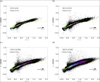 |
Fig. 2 (r – J0660) versus (r – i) colour–colour plots used to select objects with Hα excess. These plots display data for all stars from the S-PLUS DR4 MS, representing the PStotal photometry in these colours. The data are divided into four magnitude bins: (a) 13 < r ≤ 16, (b) 16 < r ≤ 17.5, (c) 17.5 < r ≤ 18.5, and (d) 18.5 < r ≤ 19.5. Objects with Hα excess are expected to be located towards the top of these diagrams. The lighter green and yellow points connected by lines represent the tracks for main-sequence and giant stars, respectively. These tracks are derived from the synthetic spectra library of Pickles (1998). The background colour gradient represents the density of objects: red indicates the highest concentration of points, followed by green, blue, and purple, which represent progressively lower concentrations. |
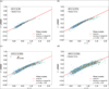 |
Fig. 3 Illustration of the selection criteria used to identify strong emission-line objects via colour–colour plots. The data shown here are from the S-PLUS field STRIPE82-0142, split into four magnitude bins, as displayed in the four panels. The thin red continuous lines show the initial linear fit to all data points (in green), while the dashed red line is the fit after applying iterative σ-clipping. Objects selected as Hα emitters are located above the dashed line. The orange star in panel c represents the cataclysmic variable (CV) FASTT 1560 (S-PLUS ID: DR4_3_STRIPE82-0142_0021237), highlighted here as an example of an Hα emitter identified by our criteria. |
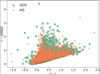 |
Fig. 4 Colour–colour diagram shows the distribution of Hα-feature sources in the (r – J0660) versus (r – i) colour–colour space. The data is divided into two populations: GDS and MS representing distinct galactic components. The GDS population, depicted by the filled circles (in green), corresponds to Hα excess sources associated with disk structures. In contrast, the MS population, represented by the squares (in orange), includes Hα excess sources primarily located in the direction of the Galactic halo and extragalactic sources. |
4 Results and analysis
Our objective is the identification of Hα excess sources within the S-PLUS footprint, leveraging the unique filter system of the survey. This effort resulted in 3637 outliers for the MS and 3319 for the GDS. The distribution of the sources with excess Hα emission in the (r – J0600) versus (r – i) colour–colour plane is depicted in Fig. 4. Square light orange symbols represent objects with Hα excess identified in the MS, while green circles denote those found in the GDS. All the sources placed above the locus of the main and giant stars exhibit an excess in the J0600 filter, attributed to the Hα excess. The broad distribution of sources on the colour–colour diagram of (r – J0660) and (r – i) indicates the selection of several types of Hα sources. These sources are likely associated with PNe, CVs, SySts, YSOs, Be stars, as well as extragalactic compact objects such as QSOs and galaxies, among others (see Fig. 2 of Gutiérrez-Soto et al. 2020).
The fractional contribution of different classes of sources to the overall sample was evaluated by cross-matching the objects’ list with the SIMBAD database9. Optical spectra available in the Sloan Digital Sky Survey (SDSS; York et al. 2000) and in the Large Sky Area Multi-Object Fiber Spectroscopic Telescope (LAMOST; Wu et al. 2011) were also explored. In all cases, positive matches between the different catalogues were considered for those sources that have an angular distance on the sky-plane within a given limit (dmax,pro j). Verification of the photometry and assessment of Hα excess in the selected objects within the disk area were conducted by cross-matching the Hα source list identified in S-PLUS with photometric data from VPHAS+ DR2.
4.1 Matches with SIMBAD sources
We identified a total of 1263 positive matches between our catalogues of Hα compact excess sources and the SIMBAD database, assuming a search radius of dmax,proj = 2 arcsec for the MS and 1 arcsec for the GDS. In the MS, the identified objects primarily fall into categories such as variable stars, predominantly cataclysmic variables and/or candidates (CataclyV*), eclipsing binaries and/or candidates (EB*), and RR Lyrae Variables (RRLyr), as well as various kinds of stars including normal stars, white dwarfs, and/or candidates (WD*). Additionally, extragalactic compact sources that exhibit redshifted lines coinciding with the J0660 filter, simulating the Hα emission line, are also present. These include AGN, Seyfert galaxies, QSOs, and other objects. It is important to note that the presence of redshifted emission lines in extragalactic sources may contribute to the identification of some of these objects as Hα excess candidates (see Table 1 for details).
For the GDS, the identified categories include emission-line stars (Em*), young stellar objects (YSOs) and candidates, which encompass T Tauri (TTau*) and Herbig Ae/Be (Ae*) star candidates. Additionally, variable stars such as cataclysmic variables (CataclyV*), eclipsing binaries (EB*), and RR Lyrae variables (RRLyr) are found, along with objects exhibiting nebular components, such as planetary nebula (PN) candidates, novae, and reflection nebulae (RfNeb), among others. As shown in Table 1, the highest number of sources in the disk belong to the Em* and young stellar objects categories, reflecting the active star formation processes in the Galactic disk.
An important consideration regarding the SIMBAD matches is that in the MS, numerous extragalactic sources with emission lines are selected due to the mapping of high latitudes in the southern sky. Conversely, for the GDS, no extragalactic sources have been selected. While the MS emphasizes extragalactic sources and diverse stellar populations, the disk region primarily showcases young stellar objects and variable stars, indicative of ongoing star formation and stellar evolution processes. In both regions, variable stars such as EB*, among others, are also present. The results are described below and listed in Table 1.
In our analysis of Hα excess sources, variable stars such as RR Lyrae stars and eclipsing binaries are frequently detected due to their tendency to exhibit significant photometric deviations in the Hα-related bands. It is important to highlight that RR Lyrae stars, which are known for their characteristic spectral features, often show Hα absorption lines. This occasionally causes them to be identified as outliers in our selection, as our criteria are sensitive to any significant deviation from expected stellar colours, whether it involves emission or absorption features. Moreover, the use of the S-PLUS filter system, with its 12 sequential filters, plays a role in detecting these short-period variables. Since both RR Lyrae and eclipsing binaries have short periods (typically hours to days), the sequential observation through S-PLUS’s filters can capture these stars at different phases of their variability. This effect can lead to apparent Hα excess due to the changes in brightness across different bands during the observation sequence. In particular, eclipsing binaries can display Hα emission due to complex interactions between the stellar components and their surrounding material. This phenomenon has been observed in systems such as the eclipsing binary VV Cephei, where periodic variations in Hα emission occur during different phases of the eclipse (Pollmann et al. 2018).
An important observation is that our selection criteria have predominantly excluded extended sources. In the MS, only 23 AGN and 9 galaxies were identified, making up approximately 3.1% and 1.2% of the total 731 SIMBAD matches (see Table 1), respectively. Additionally, we identified 143 QSOs, representing about 19.6% of the total matches. These percentages highlight the effectiveness of our selection criteria in isolating compact sources with significant Hα excess, while also illustrating the relative proportions of different astrophysical categories identified in our survey.
Positional cross-match results between S-PLUS Hα sources and the SIMBAD database.
4.2 Redshifted lines mimicking the Hα emission
According to the classification in the literature, near 20% of the Hα sources in our sample are classified as QSOs. It is important to note that the excess observed in the J0660 filter is due to QSOs whose emission lines are redshifted to the wavelength range of this filter. For instance, lines such as Hβ, Mg II 2798 Å, C III] 1909 Å, and C IV 1550 Å can contribute to this excess (see Gutiérrez-Soto et al. 2020 and the bottom of Fig. 1 of Nakazono et al. 2021, which shows the main emission lines of a quasar at different redshifts and indicates which of those fall within the J0660 filter).
This particular population of apparent Hα emitters includes AGN, Seyfert 1 galaxies, and other emission-line galaxies. In particular, within the redshift range 0.306 < z < 0.376, lines such as Hβ and [O III] 4959, 5007 Å are redshifted into the J0660 filter.
4.3 Matches with SDSS and LAMOST
Our list of Hα excess sources identified in the MS was crossmatched with the DR18 SDSS catalogue (Ahumada et al. 2020) and the DR9 LAMOST catalogue, using a 2 arcsec radius. These cross-matching identified 212 common sources (138 from SDSS and 74 from LAMOST). The procedure was restricted to the MS due to its overlap with SDSS and LAMOST areas, unlike the S-PLUS Galactic disk survey. It is noteworthy that some Hα excess sources detected by our algorithm may exhibit transient behaviour, meaning that Hα excess features might be present in spectra from one survey (SDSS or LAMOST) but not in others (S-PLUS), or vice versa. This variability is attributed to differences in observational epochs and conditions across the surveys. Upon spectroscopic examination, approximately 60% of these sources exhibited emission lines, which might include red- shifted lines other than Hα, while about 30% showed Hα-related absorption features.
Most of the objects with available spectroscopic information in SDSS and LAMOST correspond to CVs, QSOs, AGN, and variable stars. A more detailed spectroscopic characterization of these sources is beyond the scope of this paper. Also, it is worth noticing that there is a number of objects without a conclusive classification.
Figure 5 presents the SDSS (top panel) and LAMOST (middle and bottom panels) spectra, along with the corresponding S-PLUS photometry (coloured symbols), for two known CVs and one eclipsing binary. The excess in the J0660 filter is evidently produced by the Hα line. Note that the bluer emission tends to be more intense, which is consistent with the expected behavior of CVs showing strong Balmer series emission. The bottom panel of Fig. 5 displays the LAMOST spectrum and S- PLUS photometry of an eclipsing binary. The spectrum exhibits weak Hα emission, which is effectively captured by the narrow J0660 filter of S-PLUS.
Figure 6 shows the SDSS spectra and S-PLUS photometry of an RR Lyrae star with Hα in absorption. The absorption feature in Hα affects both the r-band and the J0660 filter. The apparent Hα excess observed in the r – J0660 colour index for sources with Hα absorption is due to the differential effect of the absorption feature on the broadband r filter and the narrowband J0660 filter. The Hα line lies within the r-band, so the absorption feature reduces the total flux detected, making the r band appear fainter. In contrast, the J0660 filter, shows a less pronounced reduction in flux. This difference results in a more negative r – J0660 colour index, creating an apparent Hα excess. This photometric effect is important for identifying Hα excess sources, as it indicates the presence of Hα variations, even in absorption, within various stellar objects (Fratta et al. 2021). Furthermore, most of the Hα absorption line objects in the MS (relatively high latitude) are RR Lyrae stars, as confirmed by SIMBAD, which lists 111 RR Lyrae stars in our sample. We also explore the distribution of RR Lyrae stars in the (r – J0660) versus (r – i) colour diagram, finding that these variable stars span r – J0660 values between −0.4 and 0.6. This means that a population of these stars have (r – J0660) > 0, indicating their selection (see Fig. C.1).
Figure 7 presents examples of SDSS spectra for three QSOs, where the J0660 filter captures emission from different red- shifted lines. For the QSOs in the upper panel (redshift ∼1.36), the excess corresponds to the Mg II 2798 Å line. In the middle panel (redshift ∼2.45), the excess is due to the C III] 1909 Å line. Finally, for the QSO in the bottom panel (redshift ∼3.28), the C IV 1550 Å line produces the observed excess. These plots demonstrate how the J0660 filter captures redshifted emission lines for QSOs at various redshifts.
Other extragalactic objects for which we found spectra in SDSS and LAMOST include AGN. For example, Fig. 8 displays the spectra of two nearby AGN with redshifts of approximately z ≃ 0.32 (top) and z ≃ 0.35 (bottom). In the first, the [O III] 4959, 5007 Å emission line doublet falls within our narrowband filter. For the second source, with z ≃ 0.35, the Hβ emission line lies in the J0660 filter, resulting in an observed excess.
The analysis of individual spectra reveals distinct Hα line features, including both emission and absorption at expected wavelengths, offering valuable insights into the physical characteristics and evolutionary stages of the objects. The spectral confirmation rates we present provide a conservative estimate of the selection purity. This is because our algorithm targets Hα excess sources, not strictly Hα emitters. Thus, objects with excess in the J0660 filter are selected as outliers, even if they lack a prominent Hα emission line. By referring to “Hα excess” rather than “Hα-emitters,” we highlight that our selection is based on photometric excess in the J0660 filter, rather than solely on strong Hα emission.
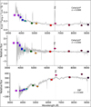 |
Fig. 5 Spectra of three objects identified as Hα excess sources using our methodology. The top panel displays the SDSS spectrum, while the middle and bottom panels show LAMOST spectra. The coloured symbols correspond to S-PLUS photometry in flux units for the following filters (from left to right): u, J0378, J0395, J0410, J0430, g, J0515, r, J0660, i, J0861, and z. The square markers represent broadband filters, while the circles denote narrowband filters. According to SIMBAD, the objects in the top and middle panels – SDSS ID J113722.24+014858.5 and LAMOST ID J232551.47-014023.5 – are classified as cataclysmic variables. The bottom panel shows an eclipsing binary star with weak Hα emission (LAMOST ID: J012119.09-001950.0). The dashed line marks the position of the Hα wavelength. |
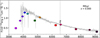 |
Fig. 6 SDSS spectrum and S-PLUS photometry of the RR Lyrae star SDSS J010045.13-010212.2, showing an Hα absorption line. |
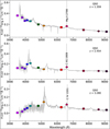 |
Fig. 7 S-PLUS photometry and SDSS spectra of three QSOs with redshifts of 1.359, 2.454, and 3.280 (from top to bottom) selected as Hα excess sources. At these redshifts, the emission lines Mg II λ2799, C III] λ1909 and C IV λ1551 are detected in the J0660 filter. The SDSS IDs of the sources are J235157.58+003610.5, J220529.34-003110.7, and J224539.94-002419.6. |
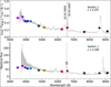 |
Fig. 8 Same as Fig. 7, but for sources with redshifts of z = 0.321 and z = 0.348. At these redshifts the [O III] λλ4959, 5007 doublet and the Hβ line are detected in the narrowband filter, generating an Hα excess. The spectra of the sources are from SDSS (top) and LAMOST (bottom) with IDs SDSS J231742.60+000535.1 and LAMOST J033429.44+000611.0, respectively. |
4.4 Evaluation of photometric colour consistency between S-PLUS and VPHAS+
We performed a comparative analysis of PSF photometric colours between the S-PLUS data from the GDS and those provided by VPHAS+ DR210. For the cross-matching, we considered a radius of 1″ and ended up with a number of 793 matches. We computed the differences in two key colour indices: (r – i) and (r – Hα). Specifically, we investigated the median difference and the median absolute deviation (MAD) of these colours to assess the consistency and agreement between the two surveys. It is worth noting that VPHAS+, as does S-PLUS, employs the r, i, and a narrowband filter (NB-659) designed to detect the Hα line, facilitating a meaningful comparison of Hα emission.
The comparison of colours reveals important insights into the consistency and reliability of S-PLUS photometry (see Fig. 9). The median difference in the r – i colour between S-PLUS and VPHAS+ was -0.21, with a MAD of 0.07. For the r – Hα colour, the median difference was 0.02 with a MAD of 0.27. These results indicate a systematic offset between the photometric colours of the two surveys, which is within the expected range considering differences in instrumentation and filter systems.
A key factor contributing to the differences in the r – Hα colour index is the distinct characteristics of the Hα filters used in S-PLUS and VPHAS+. The S-PLUS Hα filter (J0660) has an effective wavelength of 6614 Å and a width of 147 Å whereas the VPHAS+ NB-659 filter has an effective wavelength of 6588 Å and a width of 107 Å. These differences can significantly affect the measurement of Hα excess, as the narrower VPHAS+ filter captures a more restricted range of wavelengths, potentially leading to higher precision. The broader S-PLUS filter, on the other hand, may include additional continuum emission, affecting the photometric measurement. Additionally, the exposure times in the two surveys differ, with VPHAS+ using a 120- second exposure and S-PLUS using a 290-second exposure. The longer exposure time in S-PLUS allows for greater sensitivity to faint sources and potentially higher signal-to-noise ratios, contributing to the observed differences in photometric colours.
Despite the observed systematic differences, the MAD values suggest that the photometric measurements from both surveys exhibit good agreement. This consistency is crucial for cross-referencing and integrating datasets from different surveys for comprehensive astrophysical studies. The observed differences in photometric colours may result from various factors, including differences in filter characteristics, photometric calibration, and data processing techniques. Further investigations are warranted to better understand these factors’ contributions to the observed discrepancies.
4.5 Hα excess source distributions
The upper panel of Fig. 10 presents a histogram of the r-band magnitude distribution for all objects in our study from the MS. The bars represent the normalized density, allowing for comparison between different subsets. The blue bars represent Hα excess objects, while the pink bars represent all stars from the MS. The magnitude distribution for Hα excess sources shows a higher concentration at intermediate magnitudes. The lower panel of Fig. 10 focuses on the r-band magnitude distribution sources for the subset of Hα excess objects in the GDS. A noticeable large number of sources with Hα excess have magnitudes in the r-band between 13 and 13.5, something that we do not see in the stars of GDS. This implies that Hα excess objects could be intrinsically more luminous or closer to us than the general population of all stars. However, these stars are closer to the saturation limit. Therefore, we recommend exercising caution with all sources in our sample that have an r-band magnitude smaller than 13.5.
Figure C.2 shows the distribution of all Hα excess sources in Galactic latitude and longitude, along with a zoomed-in view of the GDS in the bottom panel. The distribution of objects in Galactic longitude for the MS (left panel of Fig. 11) indicates that the blue bars, representing Hα excess sources, are relatively evenly spread across the Galactic longitude, similar to the general population of stars from the MS (pink bars). Peaks are observed around Galactic longitudes of 15°, 50°, and 270°, which are also present in the general star population of the MS.
The bottom panel of Fig. C.2 and the right panel of Fig. 11 show the distribution of objects in Galactic longitude specifically within the Galactic disk or GDS. There is a noticeable concentration of Hα excess sources at specific longitudes, particularly around 243°. Additionally, there are small peaks around 225° and 268° in Galactic longitude. While Hα excess sources follow a distribution similar to that of all stars, the peaks are more pronounced for Hα excess sources.
It should be noted that the observed concentrations of Hα excess sources in certain Galactic regions may be influenced by the uneven sky coverage of the S-PLUS survey (see Fig. 6 in Herpich et al. 2024). In the MS, this effect may be more pronounced due to the lower star formation activity in high-latitude regions. For the GDS, the concentrations could be influenced by both the presence of star-forming regions and the patchy sky coverage of the survey. This limitation may lead to uneven sampling of both high-latitude and Galactic plane regions, potentially over- or under-representing the observed numbers in specific areas. Therefore, these peaks should be interpreted with this limitation in mind.
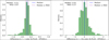 |
Fig. 9 Histograms illustrating the discrepancies in the photometric colours (r – i) and (r – Hα) between the S-PLUS and VPHAS+ surveys. The left panel depicts the differences in the (r – i) colour, while the right panel shows the differences in the r – Hα colour. The histograms reveal significant differences for the stars included in the two surveys. The median value and median absolute deviation (MAD) for each colour discrepancy are provided, offering insights into the agreement between the two datasets. |
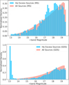 |
Fig. 10 Upper panel: distribution of r-band magnitudes for Hα excess sources (blue bars) compared to all the stars (pink curve) in the MS. Lower panel: distribution of r-band magnitudes for Hα excess sources (blue curve) compared to all stars (pink bars) in the GDS. |
5 Machine learning approaches
In this section, inspired by the goal of separating Galactic sources from extragalactic ones in our Hα excess list, we applied machine learning approaches. Our list of Hα excess sources selected in the MS of S-PLUS naturally includes extragalactic compact objects with redshifted lines detected in the J0660 filter. To classify the sources in our Hα excess list, we utilized the multi-band coverage provided by S-PLUS optical photometry.
To achieve this, we employed two unsupervised machine learning algorithms: UMAP and HDBSCAN. UMAP is used to reduce the dimensions of our data and perform a feature extraction, while HDBSCAN classifies the data based on the results from UMAP. We conducted two experiments: one using the 66 colours generated from the 12 S-PLUS filters, and a second one by adding filters from the Wide-Field Infrared Survey Explorer (WISE; Wright et al. 2010). This classification helps identify specific types of objects for subsequent spectroscopic followup. Additionally, we used a random forest algorithm to identify important features and construct colour–colour diagrams to separate the classes of objects identified by HDBSCAN. This methodology is applied to the list of Hα excess sources obtained from the MS of S-PLUS. The classification results also provide the basis for defining tentative colour criteria, which can be used to refine the separation between different classes of Hα excess sources, based on the new colour–colour diagrams proposed here.
5.1 Dimensionality reduction and clustering
5.1.1 UMAP
Uniform Manifold Approximation and Projection (UMAP; Becht et al. 2019; McInnes et al. 2020) is a dimensionality reduction algorithm designed to handle high-dimensional data while preserving its underlying structure. Unlike some other techniques, UMAP is based on a mathematical framework that combines aspects of Riemannian geometry and algebraic topology. This enables UMAP to capture both local and global relationships within the data. UMAP aims to create a low-dimensional representation that retains the intricate nonlinear relationships present in the original high-dimensional features. This process involves constructing a high-dimensional graph representation of the data and then optimizing a low-dimensional graph to match it. By doing so, UMAP effectively preserves the essential information and structure encoded in the data. This makes UMAP particularly well-suited for datasets where parameters exhibit complex nonlinear behaviour. In our analysis, we use UMAP to reduce the dimensionality of our input space, consisting of 66 colours and additional WISE bands, while retaining essential information encoded in the data.
For the implementation of the algorithm, we used the Python package umap11. UMAP has three key hyperparameters: n_neighbors, n_components, and min_dist.
The n_neighbors parameter balances local versus global structures in the data by setting the number of neighbouring points UMAP considers for each data point when learning the manifold structure. Low values of n_neighbors cause UMAP to focus on very local structures, while higher values make UMAP look at larger neighbourhoods, potentially losing fine details in favour of capturing broader patterns.
The n_components parameter, similar to the parameter used in standard dimension reduction algorithms in the scikit-learn package (Pedregosa et al. 2011), allows us to set the number of dimensions in the reduced space into which we embed the data. scikit-learn is a widely used Python library for machine learning, built on top of SciPy, and distributed under the 3-Clause BSD license. It provides implementations for many state-of-the-art machine learning techniques, making it a versatile tool for data analysis and modelling.
The min_dist parameter controls how closely UMAP can pack points together in the low-dimensional representation. Lower values result in clumpier embeddings, which are useful for clustering and capturing fine topological structures, while higher values focus on preserving broader topological structures.
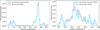 |
Fig. 11 Distribution of the objects in galactic longitude for Hα excess sources (blue bars) and all stars (pink bars) for the MS (left panel) and the GDS (right panel). |
5.1.2 HDBSCAN
After obtaining a new system of reduced variables that condenses all the information from the original variables, we utilized HDBSCAN to identify clusters within the data. This clustering approach complements the reduction achieved by UMAP, allowing for a comprehensive understanding of the underlying structure of the dataset.
Hierarchical Density-Based Spatial Clustering of Applications with Noise (HDBSCAN; Campello et al. 2013) is an unsupervised machine learning algorithm for clustering. It builds on the Density-Based Spatial Clustering of Applications with Noise (DBSCAN; Ester et al. 1996) by introducing a hierarchy to the clustering process, which allows for the extraction of persistent clusters from the hierarchical tree. HDBSCAN’s main advantage over DBSCAN is its ability to find clusters of varying densities and shapes.
For this task, we adopted the Python implementation of HDBSCAN12 (McInnes et al. 2017). The two most critical parameters are the minimum cluster size (min_cluster_size) and the minimum number of samples (min_samples). The minimum cluster size refers to the smallest group size that is considered a cluster. The minimum number of samples determines how conservative the clustering will be; larger values result in more points being classified as noise, restricting clusters to denser areas.
HDBSCAN can also classify sources as noise if they do not fit well into any cluster based on these parameters. Additionally, the algorithm relies on a distance metric, such as Euclidean distance, to measure the distance between points and determine their density. The choice of metric can significantly affect the clustering results, as it influences how distances are computed and, consequently, how clusters are formed.
5.2 Classification results
Our unsupervised UMAP model projects the data, and HDB- SCAN identifies the clusters. To ensure high-quality photometry, we required errors below 0.2 mag in all filters, reducing the sample to 2181 MS objects. This step minimizes the impact of noisy measurements, improving the performance of UMAP and HDB- SCAN. By focusing on reliable photometric data, we enhance the accuracy and robustness of the clustering, ensuring more reliable classifications of Hα excess sources.
To perform cross-validation for selecting the optimal n_neighbors and n_components parameters in UMAP, we systematically explored a range of values for these parameters. The selection of parameters n_neighbors and n_components in UMAP is critical as it directly influences the quality of the reduced-dimensional representation. Initially, we conducted exploratory data analysis to visualize the dataset in reduced dimensions using various combinations of n_neighbors and n_components. This allowed us to qualitatively assess how well UMAP preserved the underlying structure of the data.
To objectively evaluate the performance of different parameter combinations, we used two quantitative metrics: the Silhouette Score (Rousseeuw 1987) and the Davies-Bouldin Index (Davies & Bouldin 1979). The Silhouette Score measures how well-defined the clusters are in the reduced space, assessing both cohesion (how similar an object is to its own cluster) and separation (how different it is from other clusters). Higher scores indicate better separation, meaning that objects are well-matched to their own cluster and poorly matched to others. The Davies- Bouldin Index measures the average similarity between each cluster and its most similar cluster. A lower value indicates better-defined clusters. Both metrics were used to identify the optimal combination of parameters for UMAP.
A grid of tests was constructed over a range of n_neighbors (5, 10, 15, 20, 30, 50, 70, 100) and n_components (2, 3, 4, 5, 10, 20, 50) values. For each combination, UMAP was applied, followed by clustering using KMeans (Lloyd 1982), and the metrics were computed to determine the optimal parameter set. The KMeans algorithm clusters data by attempting to separate samples into n groups of equal variance by minimizing a criterion known as inertia, or the within-group sum of squares. It requires the number of clusters (n_clusters) to be specified, which was set equal to the n_components from each UMAP computation. This choice assumes that the dimensionality of the reduced space corresponds to the natural clustering structure of the data, making it a reasonable and useful strategy for exploratory data analysis. KMeans scales well to large numbers of samples and has been widely used in various fields for clustering tasks. By applying the Silhouette Score and Davies-Bouldin Index to the results, we identified the optimal parameters for both UMAP and KMeans, ensuring well-defined and separable clusters.
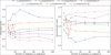 |
Fig. 12 Silhouette score (left panel) and Davies-Bouldin index (right panel) as functions of the number of neighbours (n_neighbors) for different values of UMAP components (n_components). Higher Silhouette score values and lower Davies-Bouldin index values indicate better clustering performance. |
5.2.1 Initial analysis using S-PLUS photometry
For the first experiment, we used the 66 S-PLUS colours as input parameters and applied the metric evaluation method described above. These metrics include the silhouette score, which measures cluster cohesion, and the Davies-Bouldin Index, which assesses cluster separation. Lower values of the Davies-Bouldin Index and higher silhouette scores indicate better clustering performance. After evaluating various hyperparameter combinations, we identified that setting n_neighbors = 30 and n_components = 2 yielded the highest silhouette score (0.799) and the lowest Davies-Bouldin Index (0.266). These values were subsequently adopted as the optimal hyperparameters for our analysis. For the min_dist parameter, we used the default value of 0.1. Figure 12 illustrates the behaviour of the silhouette score (left panel) and the Davies-Bouldin Index (right panel) as functions of the n_neighbors for each n_components. In the left panel, we observe that the silhouette score varies with n_neighbors, with the best performance achieved at n_neighbors = 30 and n_components = 2. The right panel shows the Davies-Bouldin Index, which decreases consistently for these hyperparameters, confirming their optimality.
Following dimensionality reduction with UMAP, the resultant variables were utilized to construct HDBSCAN models. We experimented various combination for the minimum cluster size and minimum number of samples parameters. We ended up with the optimal value of 2 and 50, respectively. Euclidean metric was employed for distance calculations throughout.
The left panel of Fig. 13 shows the distribution of the new variables in UMAP space, resulting from applying it to the 66 S-PLUS colours of the Hα excess objects for the MS. The colour bar indicates the r magnitude, highlighting the bright and faint sources. Visually, it is possible to distinguish at least four groups, with the small clusters located in the upper left of the diagram tending to be fainter. The right panel of the Fig. 13 shows the same plot but with the results of applying HDBSCAN using the parameters mentioned above. HDBSCAN identified four groups. Table D.1 provides the number of objects in each group. To further understand the nature of each group, we examined their SIMBAD counterparts, which are also detailed in the Table D.1:
Group 0 contains 58 objects, 22 of which are matched in SIMBAD. The majority are QSOs (19), with the remaining objects including one galaxy, one radio source, and one QSO candidate. This composition suggests that Group 0 primarily consists of extragalactic sources, with a redshift distribution peak around 2.45. It is worth noting that the spectral characteristics of QSOs (a type of AGN) differ significantly from typical galaxies; while starburst galaxies show strong extinction at blue wavelengths, the QSO spectrum rises sharply towards the blue, indicative of the high-energy processes associated with active galactic nuclei.
Group 1 contains 166 objects, 149 of which have entries in the database. This group is predominantly composed of RR Lyrae stars (107), followed by eclipsing binaries (19), various types of pulsating variables (9), and a few other stellar objects, including 2 QSOs. This group appears to represent objects with Hα in absorption, as it is well known that RR Lyrae stars exhibit Hα absorption lines.
Group 2 includes 1539 objects, 323 of which are catalogued in SIMBAD. The majority are eclipsing binaries (275), followed by a few stars (10), QSOs (9), and a small number of cataclysmic variables and RR Lyrae stars. In this context, the QSOs are AGN without detectable Hα emission within the S-PLUS wavelength range (or where the SDSS spectra do not cover the Hα line). This group is thus characterized by the significant presence of binary star systems and various types of variable stars.
Group 3 consists of 93 objects, 42 of which are matched in the database. According to SIMBAD, the majority are labeled as QSOs (17), along with Seyfert 1 galaxies (10) and other classifications such as AGN candidates, radio sources, and a few galaxies. However, upon inspecting the spectra of several of these QSOs, we find that the line observed within the S-PLUS J0660 filter corresponds to [O III] and/or Hβ, rather than Hα. Given the narrow redshift range (0.31 to 0.37), these characteristics suggest that the objects in this group are better classified as AGN, not QSOs. This may indicate a misclassification in SIMBAD, where sources labelled as QSOs in this group likely correspond to AGN.
Group 4 includes 325 objects, 143 of which are recorded in the database. This group has a high concentration of QSOs (78) and cataclysmic variables (25). Additionally, it features a mix of blue stars, AGN, radio sources, and white dwarf candidates. The extragalactic objects in this group show a peak in the redshift distribution around 1.35. It is expected that CVs are located closer to the QSOs than to Galactic sources in the UMAP variable space due to their photometric characteristics, which can resemble those of QSOs in certain features, despite the spectral differences (Scaringi et al. 2013).
In summary, our application of UMAP and HDBSCAN to the Hα excess sources has effectively identified distinct groups with varying astrophysical characteristics using S-PLUS photometry. The classification successfully differentiates extragalactic sources, such as QSOs and AGN, from galactic sources, including variable stars and binary systems. However, distinguishing Galactic cataclysmic variables from QSOs with redshifts around 1.35 remains challenging. Importantly, our results suggest that objects with J0660 - r colour excess due to emission lines can be distinguished from those with excess caused by Hα absorption lines, mainly RR Lyrae stars.
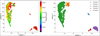 |
Fig. 13 UMAP dimension reduction applied to the MS from S-PLUS data. The left panel shows the UMAP result using only the S-PLUS colours as input parameters, with the colour bar indicating the r magnitude. The right panel displays the result after applying HDBSCAN clustering, revealing five distinct groups. |
5.2.2 Integration of S-PLUS and WISE photometry
The second experiment incorporated the W1 and W2 filters from the WISE survey. These filters were selected because they provide the best sensitivity and reliability for detecting sources with infrared excess or thermal emission (Nakazono et al. 2021). To include these data, we cross-matched the Hα sources from the Main Survey of S-PLUS with the ALLWISE catalogue (Cutri et al. 2013) using a search radius of 2 arcsec. This radius was chosen considering the broader point-spread function (PSF) of WISE compared to S-PLUS, as discussed in Nakazono et al. (2021). This process initially yielded 3173 matches, which were reduced to 1910 after applying photometric quality cuts, including errors smaller than 0.5 magnitudes in W1 and W2 and equivalent constraints for S-PLUS filters.
Additional colours were constructed by combining WISE bands (W1 and W2) with S-PLUS broadband filters, such as W1–W2, W1–u, W2–u, W1–g, and so on. This expanded the parameter space from 66 to 77 variables, enriching the dataset and enhancing the performance of machine learning models in characterizing the physical properties of the Hα sources. We identified optimal parameters for UMAP as n_neighbors = 50 and n_components = 2, based on the silhouette score and the Davies-Bouldin Index. For HDBSCAN, we employed min_cluster_size = 50 and min_samples = 5.
Figure 14 shows the results of the reduction in dimensionality and the groups identified by applying UMAP followed by HDBSCAN, using the input parameters described in the previous paragraph. On this occasion, HDBSCAN found five groups and one objects that were classified as noise. Table D.1 summarizes these results:
Group 0 contains 1437 objects, 424 of which correspond to entries in the SIMBAD database. Among these, 262 are eclipsing binaries (EB*), followed by 98 RR Lyrae stars (RRLyr). Other objects include EB* candidates, stars, pulsating variables, and a few QSOs. This group predominantly consists of variable stars and a small number of extragalactic sources.
Group 1 includes 59 objects, 23 of which are matched with SIMBAD. The majority are QSOs (20), with a few other objects, for example a galaxy, a radio source, and a QSO candidate. This group mainly represents extragalactic sources, particularly active galactic nuclei. The redshift distribution has a peak around 2.45. This group resembles Group 0 from the previous case (without WISE analysis), albeit with one additional QSO.
Group 2 consists of 93 objects, with 43 identified in the database. The group is primarily composed of QSOs (18), Seyfert 1 galaxies (10), and AGN candidates, with some galaxies and radio sources. This indicates a strong presence of active galactic nuclei and other extragalactic objects. The redshift distribution for extragalactic objects in this group ranges approximately from 0.31 to 0.37. This group is analogous to Group 3 from the previous analysis (without WISE data).
Group 3 includes 51 objects, with 36 matches in SIMBAD. The majority are cataclysmic variables (24), with a few CV candidates, hot subdwarf candidates, and white dwarf candidates. This group is largely composed of cataclysmic variables and related stellar objects.
Group 4 contains 269 objects, 100 of which are matched with the database. The majority are QSOs (83), with a mix of blue stars, AGN, radio sources, stars, and galaxies. This group shows a variety of astrophysical phenomena, both stellar and extragalactic, with a redshift distribution peaking around 1.35. It is similar to Group 4 from the previous analysis using only S- PLUS data. In the S-PLUS-only group, the majority of objects are QSOs and cataclysmic variables, while the S-PLUS + WISE group contains more QSOs but no cataclysmic variables. The photometric characteristics of CVs in S-PLUS resemble those of QSOs, explaining why they cluster closer to QSOs than to Galactic sources in the UMAP variable space. The inclusion of WISE data likely contributed to the increase in QSOs by providing infrared information that helps differentiate extragalactic objects.
In summary, the inclusion of WISE filters in our analysis has significantly enhanced the clustering of Hα excess sources. The integration of WISE data has allowed for a more precise differentiation between galactic and extragalactic sources, enriching our understanding of the objects in our dataset. Notably, it has facilitated the separation of cataclysmic variables from QSOs with redshifts around 1.35. For detailed insights, refer to Sect. 4 where the redshifted emission lines of extragalactic objects are highlighted in the J0660 filter. However, it is important to note that the addition of WISE data has introduced challenges in identifying the group of RR Lyrae stars using HDBSCAN.
Uncertainties in photometric colours of variable stars based on single, random observations are inherently biased due to the stars’ intrinsic variability. This effect is more pronounced with an increase in the amplitude of variability, as seen in classes of stars such as RR Lyrae and Mira variables, which typically exhibit amplitudes higher than 0.3 to 2 magnitudes for RR Lyrae stars Chandra X-ray Observatory. The S-PLUS survey offers a significant advantage in this regard, as its 12 photometric wavebands are observed nearly simultaneously within approximately 1.5 hours SPLUS. Consequently, these observations are closely spaced in phase for variable stars.
For instance, RR Lyrae stars (RRab subtype), which have periods of approximately 0.5 days Chandra X-ray Observatory, will have all 12 S-PLUS wavebands captured within a phase range of ≃0.1. This minimizes the variability effects on the observed photometric colours and ensures a more precise and reliable measurement of stellar parameters derived from these data. In contrast, random or non-simultaneous observations are likely to result in larger uncertainties due to phase mismatches, particularly for variable stars with significant amplitude changes over short timescales.
When S-PLUS wavebands are combined with external data, such as WISE wavebands, the phase mismatch becomes a critical source of uncertainty. WISE observations, which are not time-synchronized with S-PLUS, can introduce errors because the observed phases of variable stars in the combined dataset will be random. As a result, the derived colours and parameters will suffer from increased scatter and reduced precision. Therefore, we attribute the improved performance of models relying solely on S-PLUS observations to the reduced uncertainties in colours achieved by observing all wavebands in a near-simultaneous manner. This emphasizes the importance of phase-coherent photometric observations for the precise characterization of variable stars, especially those with significant amplitude variability.
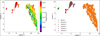 |
Fig. 14 Similar to Fig. 13, but with additional features created using the W1 and W2 bands from WISE. The left panel shows the UMAP result, with the colour bar indicating the r magnitude, and the right panel shows the HDBSCAN clustering result, identifying five distinct groups. |
5.3 Extracting main features: Colour analysis
In this section, we focus on the colours derived from the S- PLUS and WISE filters, which are effective in distinguishing the different groups of Hα excess objects identified by the combined UMAP and HDBSCAN analysis of the MS S-PLUS data.
In the MS Hα excess list, we identified extragalactic sources with higher redshifts, where blueward emission lines are red- shifted to wavelengths near Hα, resulting in an apparent Hα excess in the J0660 filter. By incorporating the WISE filters to create additional colours for the unsupervised machine learning models, we achieved better separation of extragalactic sources from Galactic sources (see Sect. 5.2 for more details).
We used the classifications made by combining UMAP and HDBSCAN to create random forest (Breiman 2001) models and identified the most important features, specifically the colours that contribute to the separation or classification of the classes of objects. The random forest algorithm is an ensemble learning method that builds multiple decision trees during the training phase. Each tree is trained on a random subset of the data and a random subset of features, which helps reduce overfitting and improves model generalization. During prediction, the results from all trees are aggregated by voting (for classification) or averaging (for regression), providing more stable and accurate predictions. Random forests are widely used for classification and regression tasks, known for their ability to handle complex data and offer reliable results. We implemented Random Forest algorithm, using 66 S-PLUS colours plus 11 additional colours generated with the W1 and W2 filters as input parameters, and labels generated by HDBSCAN.
The dataset used in this study exhibited a class imbalance: cluster 0 (1437 points), cluster 1 (59 points), cluster 2 (93 points), cluster 3 (51 points), and cluster 4 (269 points). To address this imbalance, we used the class_weight='balanced' parameter in the random forest algorithm. The classifier achieved an F1 Macro Average of 0.95 (±0.08) during 5-fold cross-validation. This high score, along with low variability, indicates that the model effectively handles the imbalance and consistently classifies the different clusters. The Macro F1 score is the average of the F1 scores calculated for each class, where each class is given equal weight, regardless of its frequency. The F1 score itself is the harmonic mean of precision and recall, providing a single metric that balances both. This metric is particularly useful in the presence of class imbalance, as it ensures that each class contributes equally to the overall score. For more details, see Sokolova & Lapalme (2009). The random forest algorithm and Macro F1 score were implemented using the scikit-learn package.
After performing the model, we accessed the feature importances using feature_importances from the random forest package. Figure 15 shows the top 20 feature importances and their respective scores, indicating the colours that contributed most to clustering the different classes of objects identified by UMAP + HDBSCAN.
Now that we have identified the important colours, we used the pairplot routine in the seaborn package (Waskom 2021) to generate all possible colour–colour diagrams using the top 20 features. Seaborn is a Python library designed to simplify the creation of statistical graphics. It extends Matplotlib and integrates seamlessly with pandas, making it particularly effective for handling and visualizing structured datasets. The pairplot function is especially useful for creating scatterplot matrices, allowing the simultaneous visualization of pairwise relationships between multiple features in the data. This allowed us to identify the colour–colour diagrams that best separate the different classes of objects and choose the most effective ones.
Figure 16 shows nine colour–colour diagrams that we selected for their ability to better separate the groups found in our Hα excess sources list. These diagrams are based on the key features of importance, and we aimed to utilize nearly all of the 20 colours. Tentative colour cuts are presented in the Fig. 16 to differentiate the various classes of Hα sources.
This exercise demonstrates that using specific colour–colour diagrams with selected filters can effectively classify objects. By relying on a few key colours instead of all 12 S-PLUS filters and 2 WISE filters required for the machine learning in Sect. 5.2, we can reduce the number of necessary observations. This approach is advantageous because not all objects have complete photometry in all filters, and some magnitudes may not meet the clean criteria, reducing the number of objects available for classification. Consequently, using a few specific colour criteria enables the classification of more objects, as it circumvents the need for complete data across all filters.
This analysis provides a practical framework for classifying Hα excess sources without relying on complex algorithms. The proposed colour–colour diagrams enable the direct application of selection criteria, offering an effective method to distinguish between different classes based on the key features identified. Building on the methodology of Corradi et al. (2008) for the (r - i) versus (r-Hα) diagram, we extend it with new and effective colour combinations. These criteria provide a valuable tool for identifying distinct classes of Hα excess sources, as shown in Table D.1, and can aid in targeted spectroscopic follow-ups.
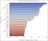 |
Fig. 15 Top 20 feature importances identified by the random forest model, showing the colours that contributed most significantly to the clustering of Hα excess objects using UMAP + HDBSCAN. The importance scores indicate the relative impact of each colour on the classification of different object classes. |
6 Conclusions
In this study, we have leveraged the S-PLUS project to analyse and classify Hα excess sources in the southern sky, resulting in the following key conclusions:
We identified 6956 Hα excess candidates by using the narrow J0660 filter in combination with the broad r and i filters from S-PLUS. This included 3637 candidates from the high-latitude MS and 3319 from the GDS.
Cross-referencing with the SIMBAD database enabled us to explore the types of objects in our list, identifying various emission-line objects such as EM stars, YSOs, Be stars, CVs, PNe, and others. We also identified QSOs, non-local galaxies, and objects with Hα in absorption, including RR Lyrae stars, primarily within the MS. The higher detection of RR Lyrae stars (111) in the MS compared to the GDS (8), based on SIMBAD, aligns with their expected distribution in older stellar populations.
Validation with spectroscopic data from LAMOST and SDSS showed that approximately 60% of the spectra exhibit Hα emission lines, while around 30% show Hα in absorption in the MS. This comparison indicates the general accuracy of our classifications and supports the reliability of our Hα excess source identifications. Furthermore, the VPHAS+ data for the GDS are consistent with our findings.
The S-PLUS 12-filter system facilitates the detection of RR Lyrae stars and eclipsing binaries as Hα excess sources, capturing their short-period variability through the sequential exposures of specific filters, such as r and J0660. This makes S-PLUS particularly suited for identifying and studying such variables, enabling the detailed analysis of their photometric behaviour and potential Hα features.
The use of machine learning techniques, specifically UMAP for dimensionality reduction and HDBSCAN for clustering, significantly enhanced our analysis of Hα excess sources. The 12 S-PLUS filters allowed the effective differentiation between Galactic Hα-emission objects and extragalactic sources, as well as those with Hα in absorption, such as RR Lyrae stars. However, the classification of CVs versus QSOs or AGN, particularly with redshifts around 1.35, remained challenging. The similarity in the photometric characteristics of these objects made the boundaries between them less distinct, highlighting the inherent complexity in separating these sources, even when applying machine learning techniques with S-PLUS colours.
The integration of WISE filter data significantly improved the clustering process, leading to a more accurate separation between extragalactic and Galactic sources. In particular, it facilitated the differentiation between CVs and QSOs, especially for objects with redshifts around 1.35, where their photometric characteristics previously overlapped. This enhancement enabled the clear separation of CVs from QSOs, refining the classification of these sources. Additionally, the infrared data allowed the identification of specific groups corresponding to AGN or QSOs at particular redshifts, clearly separating them from Galactic sources. Certain groups identified in the clustering process were distinctly linked to AGN or QSOs at specific redshifts, underscoring the value of combining optical and infrared data to resolve subtle differences in photometric signatures. However, the integration of WISE data also introduced challenges in classifying RR Lyrae stars, as the combination of optical and infrared data introduced noise in the clustering algorithm, complicating their precise classification.
Using data from the S-PLUS Main Survey (MS) and WISE, we constructed new effective colour–colour diagrams. By applying a random forest model to the results of clustering with UMAP and HDBSCAN, we identified key photometric features that differentiate the various classes of Hα excess sources. Additionally, tentative colour criteria are proposed within these colour–colour diagrams, enabling a preliminary classification of sources without the need for complex algorithms.
Our study used observational and analytical techniques to gain valuable insights into Hα excess sources. Although challenges were encountered, particularly with RR Lyrae stars and certain extragalactic objects, our methods provided a robust framework for understanding Hα excess phenomena. Our findings underscore the versatility of S-PLUS for identifying and understanding Hα excess phenomena, demonstrating its potential for future applications in different sky regions and astrophysical environments. Future research should focus on expanding sample sizes and incorporating additional spectroscopic data to further refine classifications. Applying these methods to other sky regions or wavelengths could enhance our understanding of Hα excess sources and their astrophysical contexts.
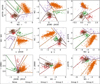 |
Fig. 16 Examples of colour–colour diagrams using the top 20 features identified by the random forest model. These diagrams show the separation of different classes of objects from the Hα excess sources list. The selected diagrams illustrate effective clustering achieved through UMAP + HDBSCAN, highlighting key colours that contribute to classification. The coloured lines represent tentative colour cuts for separating different classes of Hα excess sources. |
Data availability
The catalogues are available at the CDS via anonymous ftp to cdsarc.cds.unistra.fr (130.79.128.5) or via https://cdsarc.cds.unistra.fr/viz-bin/cat/J/A+A/695/A104
Acknowledgements
We would like to thank the anonymous referee for their detailed report on the manuscript, which significantly helped us improve the paper. LAG-S acknowledges funding for this work from CONICET and FAPESP grants 2019/26412-0. RLO acknowledges financial support from the Brazilian institutions CNPq (PQ-312705/2020-4 and 445047/2024-0) and FAPESP (#2020/00457-4). DRG acknowledges grants from FAPERJ (E-26/211.527/2023) and CNPq (315307/2023-4). LLN thanks Fundação de Amparo à Pesquisa do Estado do Rio de Janeiro (FAPERJ) for granting the postdoctoral research fellowship E-40/2021(280692). M.B.F. acknowledges financial support from the National Council for Scientific and Technological Development (CNPq) Brazil (grant number: 307711/2022-6). S.D. acknowledges CNPq/MCTI for grant 306859/2022-0. PKH gratefully acknowledges the Fundação de Amparo à Pesquisa do Estado de São Paulo (FAPESP) for the support grant 2023/14272-4. CL-D acknowledges a grant from the ESO Comite Mixto 2022. SP is supported by the international Gemini Observatory, a program of NSF NOIRLab, which is managed by the Association of Universities for Research in Astronomy (AURA) under a cooperative agreement with the U.S. National Science Foundation, on behalf of the Gemini partnership of Argentina, Brazil, Canada, Chile, the Republic of Korea, and the United States of America. AAC acknowledges financial support from the Severo Ochoa grant CEX2021- 001131-S funded by MCIN/AEI/10.13039/501100011033. The S-PLUS project, including the T80- South robotic telescope and the S-PLUS scientific survey, was founded as a partnership between the Fundação de Amparo à Pesquisa do Estado de São Paulo (FAPESP), the Observatório Nacional (ON), the Federal University of Sergipe (UFS), and the Federal University of Santa Catarina (UFSC), with important financial and practical contributions from other collaborating institutes in Brazil, Chile (Universidad de La Serena), and Spain (Centro de Estudios de Física del Cosmos de Aragón, CEFCA). We further acknowledge financial support from the São Paulo Research Foundation (FAPESP), the Brazilian National Research Council (CNPq), the Coordination for the Improvement of Higher Education Personnel (CAPES), the Carlos Chagas Filho Rio de Janeiro State Research Foundation (FAPERJ), and the Brazilian Innovation Agency (FINEP). Funding for the SDSS and SDSS-II has been provided by the Alfred P. Sloan Foundation, the Participating Institutions, the National Science Foundation, the U.S. Department of Energy, the National Aeronautics and Space Administration, the Japanese Monbukagakusho, the Max Planck Society, and the Higher Education Funding Council for England. The SDSS Web Site is http://www.sdss.org/. The SDSS is managed by the Astrophysical Research Consortium for the Participating Institutions. The Participating Institutions are the American Museum of Natural History, Astrophysical Institute Potsdam, University of Basel, University of Cambridge, Case Western Reserve University, University of Chicago, Drexel University, Fermilab, the Institute for Advanced Study, the Japan Participation Group, Johns Hopkins University, the Joint Institute for Nuclear Astrophysics, the Kavli Institute for Particle Astrophysics and Cosmology, the Korean Scientist Group, the Chinese Academy of Sciences (LAMOST), Los Alamos National Laboratory, the Max-Planck-Institute for Astronomy (MPIA), the Max-PlanckInstitute for Astrophysics (MPA), New Mexico State University, Ohio State University, University of Pittsburgh, University of Portsmouth, Princeton University, the United States Naval Observatory, and the University of Washington. Guoshoujing Telescope (the Large Sky Area Multi-Object Fiber Spectroscopic Telescope LAMOST) is a National Major Scientific Project built by the Chinese Academy of Sciences. Funding for the project has been provided by the National Development and Reform Commission. LAMOST is operated and managed by the National Astronomical Observatories, Chinese Academy of Sciences. Scientific software and databases used in this work include TOPCAT (http://www.star.bristol.ac.uk/~mbt/topcat/; (Taylor 2005)), simbad and vizier from Strasbourg Astronomical Data Center (CDS; cdsarc.cds.unistra.fr) and the following python packages: numpy, astropy, matplotlib, seaborn, pandas, scikit-learn, hdbscan, umap.
Appendix A SExtractor and PSFex parameters
Table A.1 summarizes the key SExtractor and PSFex parameters used in this work.
SExtractor and PSFex input parameters.
Appendix B Colour-colour diagrams and Hα selection for the GDS
This appendix presents two colour–colour diagrams: (r – J0660) versus (r – i) for the GDS. Figure B.1 shows the diagram for the full sample after applying the cleaned criteria described in Sect. 3, while Fig. B.2 focuses on the S-PLUS field STRIPE82- 0142, divided into four magnitude bins. This figure illustrates the process of identifying Hα excess candidates for the GDS.
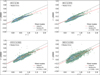 |
Fig. B.2 Colour-colour diagram of the stars located at field SPLUS-d288 of the GDS, similar to those found in Fig. 3. The red lines represent the original fit to all data, while the black dashed lines represent the final fits to the upper locus of points, obtained by applying an iterative fitting process to the initial fit. |
Appendix C Supplementary analyses
This appendix provides supplementary analyses for two related but distinct components of this study: (1) RR Lyrae stars identified through a cross-match S-PLUS with an external RR Lyrae catalogue, and (2) the broader population of Hα excess objects detected in our S-PLUS data.
Appendix C.1 RR Lyrae stars in the (r – J0660) versus (r – i) diagram
To better understand the photometric properties of RR Lyrae stars and their relationship to Hα excess sources, we performed a cross-match between the extensive RR Lyrae catalogue from Greer et al. (2017) (containing 4963 objects) and the S-PLUS dataset. This resulted in 375 matches. Figure C.1 shows the distribution of these RR Lyrae stars in the (r – J0660) versus (r – i) diagram. Notably, a subset of these stars exhibits properties consistent with Hα excess, which explains their inclusion in our Hα excess sample. The horizontal dashed line indicates the (r – J0660) = 0 value, providing a reference for interpreting the colour distribution.
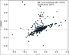 |
Fig. C.1 Distribution of RR Lyrae stars from the catalogue of Greer et al. (2017) matched with S-PLUS data, shown in the (r – J0660) vs (r – i) diagram. The horizontal dashed line indicates the (r – J0660) = 0 value. |
Appendix C.2 Spatial distribution of Hα excess objects
We also examined the spatial distribution of the broader population of Hα excess objects detected in our S-PLUS data. Figure C.2 illustrates the distribution of all Hα excess objects in Galactic longitude and latitude coordinates. The upper panel shows the full sample, while the lower panel provides a zoomedin view of their distribution in the Galactic Disk Survey (GDS).
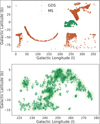 |
Fig. C.2 Distribution of Hα excess objects in Galactic longitude and latitude coordinates. The upper panel shows all the Hα sources selected, and the lower panel is a zoomed-in view of their distribution in the GDS. |
Appendix D Machine learning clustering results
To provide a comprehensive overview of the clustering results obtained using UMAP and HDBSCAN for the MS, we present in Table D.1 a summary of the number of objects in each identified group. The clustering was performed for two experiments: first using S-PLUS filters alone and second using a combination of S-PLUS and WISE filters. Additionally, we include the number of objects with SIMBAD matches and a brief description of their classifications based on SIMBAD identifications, providing insights into the distribution of sources identified through the clustering process.
Clustering results for Hα excess sources in the Main Survey (MS).
References
- Abril, J., Schmidtobreick, L., Ederoclite, A., & López-Sanjuan, C. 2020, MNRAS, 492, L40 [NASA ADS] [CrossRef] [Google Scholar]
- Ahumada, R., Prieto, C. A., Almeida, A., et al. 2020, ApJS, 249, 3 [Google Scholar]
- Akras, S. 2023, MNRAS, 519, 6044 [NASA ADS] [CrossRef] [Google Scholar]
- Akras, S., Guzman-Ramirez, L., & Gonçalves, D. R. 2019a, MNRAS, 488, 3238 [NASA ADS] [CrossRef] [Google Scholar]
- Akras, S., Guzman-Ramirez, L., Leal-Ferreira, M. L., & Ramos-Larios, G. 2019b, ApJS, 240, 21 [NASA ADS] [CrossRef] [Google Scholar]
- Akras, S., Leal-Ferreira, M. L., Guzman-Ramirez, L., & Ramos-Larios, G. 2019c, MNRAS, 483, 5077 [NASA ADS] [CrossRef] [Google Scholar]
- Akras, S., Gonçalves, D. R., Alvarez-Candal, A., & Pereira, C. B. 2021, MNRAS, 502, 2513 [CrossRef] [Google Scholar]
- Almeida-Fernandes, F., SamPedro, L., Herpich, F. R., et al. 2022, MNRAS, 511, 4590 [NASA ADS] [CrossRef] [Google Scholar]
- Barentsen, G., Vink, J. S., Drew, J. E., et al. 2011, MNRAS, 415, 103 [CrossRef] [Google Scholar]
- Barentsen, G., Farnhill, H. J., Drew, J. E., et al. 2014, MNRAS, 444, 3230 [NASA ADS] [CrossRef] [Google Scholar]
- Becht, E., McInnes, L., Healy, J., et al. 2019, Nat. Biotechnol., 37, 38 [CrossRef] [Google Scholar]
- Benitez, N., Dupke, R., Moles, M., et al. 2014, arXiv e-prints [arXiv:1403.5237] [Google Scholar]
- Bertin, E. 2011, in Astronomical Society of the Pacific Conference Series, 442, Astronomical Data Analysis Software and Systems XX, eds. I. N. Evans, A. Accomazzi, D. J. Mink, & A. H. Rots, 435 [NASA ADS] [Google Scholar]
- Bertin, E., & Arnouts, S. 1996, A&AS, 117, 393 [NASA ADS] [CrossRef] [EDP Sciences] [Google Scholar]
- Blair, W. P., & Long, K. S. 2004, ApJS, 155, 101 [NASA ADS] [CrossRef] [Google Scholar]
- Bom, C. R., Cortesi, A., Lucatelli, G., et al. 2021, MNRAS, 507, 1937 [CrossRef] [Google Scholar]
- Bonoli, S., Marín-Franch, A., Varela, J., et al. 2021, A&A, 653, A31 [NASA ADS] [CrossRef] [EDP Sciences] [Google Scholar]
- Breiman, L. 2001, Mach. Learn., 45, 5 [Google Scholar]
- Campello, R. J. G. B., Moulavi, D., & Sander, J. 2013, in Advances in Knowledge Discovery and Data Mining, eds. J. Pei, V. S. Tseng, L. Cao, H. Motoda, & G. Xu (Berlin, Heidelberg: Springer Berlin Heidelberg), 160 [Google Scholar]
- Cenarro, A. J., Moles, M., Cristóbal-Hornillos, D., et al. 2019, A&A, 622, A176 [NASA ADS] [CrossRef] [EDP Sciences] [Google Scholar]
- Coelho, P. R. T. 2014, MNRAS, 440, 1027 [Google Scholar]
- Cook, D. O., Kasliwal, M. M., Van Sistine, A., et al. 2019, ApJ, 880, 7 [Google Scholar]
- Corradi, R. L. M., & Giammanco, C. 2010, A&A, 520, A99 [NASA ADS] [CrossRef] [EDP Sciences] [Google Scholar]
- Corradi, R. L. M., Rodríguez-Flores, E. R., Mampaso, A., et al. 2008, A&A, 480, 409 [NASA ADS] [CrossRef] [EDP Sciences] [Google Scholar]
- Corradi, R. L. M., Sabin, L., Munari, U., et al. 2011, A&A, 529, A56 [NASA ADS] [CrossRef] [EDP Sciences] [Google Scholar]
- Cutri, R. M., Wright, E. L., Conrow, T., et al. 2013, Explanatory Supplement to the AllWISE Data Release Products by R. M. Cutri et al. [Google Scholar]
- Davies, D. L., & Bouldin, D. W. 1979, IEEE Trans. Pattern Anal. Mach. Intell., PAMI-1, 224 [CrossRef] [Google Scholar]
- Davies, R. D., Elliott, K. H., & Meaburn, J. 1976, MmRAS, 81, 89 [NASA ADS] [Google Scholar]
- Drew, J. E., Greimel, R., Irwin, M. J., et al. 2005, MNRAS, 362, 753 [NASA ADS] [CrossRef] [Google Scholar]
- Drew, J. E., Greimel, R., Irwin, M. J., & Sale, S. E. 2008, MNRAS, 386, 1761 [Google Scholar]
- Drew, J. E., Gonzalez-Solares, E., Greimel, R., et al. 2014, MNRAS, 440, 2036 [Google Scholar]
- Ester, M., Kriegel, H.-P., Sander, J., & Xu, X. 1996, in Proceedings of 2nd International Conference on Knowledge Discovery and Data Mining (KDD-96), 226 [Google Scholar]
- Fratta, M., Scaringi, S., Drew, J. E., et al. 2021, MNRAS, 505, 1135 [NASA ADS] [CrossRef] [Google Scholar]
- Frew, D. J. 2008, PhD thesis, Department of Physics, Macquarie University, NSW 2109, Australia [Google Scholar]
- Fukugita, M., Ichikawa, T., Gunn, J. E., et al. 1996, AJ, 111, 1748 [Google Scholar]
- González-Lópezlira, R. A., Lomelí-Núñez, L., Álamo-Martínez, K., et al. 2017, ApJ, 835, 184 [CrossRef] [Google Scholar]
- González-Lópezlira, R. A., Lomelí-Núñez, L., Ordenes-Briceño, Y., et al. 2022, ApJ, 941, 53 [CrossRef] [Google Scholar]
- Greer, P. A., Payne, S. G., Norton, A. J., et al. 2017, A&A, 607, A11 [NASA ADS] [CrossRef] [EDP Sciences] [Google Scholar]
- Groot, P. J., Verbeek, K., Greimel, R., et al. 2009, MNRAS, 399, 323 [NASA ADS] [CrossRef] [Google Scholar]
- Gutiérrez-Soto, L. A., Gonçalves, D. R., Akras, S., et al. 2020, A&A, 633, A123 [Google Scholar]
- Gutiérrez-Soto, L. A., Mari, M. B., Weidmann, W. A., & Faifer, F. R. 2024, New A, 109, 102207 [CrossRef] [Google Scholar]
- Herpich, F. R., Almeida-Fernandes, F., Oliveira Schwarz, G. B., et al. 2024, A&A, 689, A249 [NASA ADS] [CrossRef] [EDP Sciences] [Google Scholar]
- Jacoby, G. H., Kronberger, M., Patchick, D., et al. 2010, PASA, 27, 156 [Google Scholar]
- Jaiswal, S., & Omar, A. 2016, MNRAS, 462, 92 [CrossRef] [Google Scholar]
- Kalari, V. M., Vink, J. S., Drew, J. E., et al. 2015, MNRAS, 453, 1026 [CrossRef] [Google Scholar]
- Kron, R. G. 1980, ApJS, 43, 305 [Google Scholar]
- Lloyd, S. 1982, IEEE Trans. Inform. Theory, 28, 129 [Google Scholar]
- Lomelí-Núñez, L., Mayya, Y. D., Rodríguez-Merino, L. H., Ovando, P. A., & Rosa-González, D. 2022, MNRAS, 509, 180 [Google Scholar]
- Marín-Franch, A., Chueca, S., Moles, M., et al. 2012, SPIE Conf. Ser., 8450, 84503S [Google Scholar]
- McInnes, L., Healy, J., & Astels, S. 2017, J. Open Source Softw., 2 [Google Scholar]
- McInnes, L., Healy, J., & Melville, J. 2020, arXiv e-prints [arXiv:1802.03426] [Google Scholar]
- Mendes de Oliveira, C., Ribeiro, T., Schoenell, W., et al. 2019, MNRAS, 489, 241 [NASA ADS] [CrossRef] [Google Scholar]
- Merc, J., Gàlis, R., & Wolf, M. 2019, Eruptive Stars Inform. Lett., 41, 78 [Google Scholar]
- Merc, J., Mikołajewska, J., Gromadzki, M., et al. 2020, A&A, 644, A49 [NASA ADS] [CrossRef] [EDP Sciences] [Google Scholar]
- Merc, J., Gális, R., Wolf, M., et al. 2021, MNRAS, 506, 4151 [NASA ADS] [CrossRef] [Google Scholar]
- Merc, J., Gális, R., Wolf, M., et al. 2022, MNRAS, 510, 1404 [Google Scholar]
- Mikołajewska, J., Caldwell, N., & Shara, M. M. 2014, MNRAS, 444, 586 [CrossRef] [Google Scholar]
- Mikołajewska, J., Shara, M. M., Caldwell, N., Iłkiewicz, K., & Zurek, D. 2017, MNRAS, 465, 1699 [CrossRef] [Google Scholar]
- Miszalski, B., & Mikołajewska, J. 2014, MNRAS, 440, 1410 [NASA ADS] [CrossRef] [Google Scholar]
- Miszalski, B., Acker, A., Moffat, A. F. J., Parker, Q. A., & Udalski, A. 2009, A&A, 496, 813 [NASA ADS] [CrossRef] [EDP Sciences] [Google Scholar]
- Monguió, M., Greimel, R., Drew, J. E., et al. 2020, A&A, 638, A18 [NASA ADS] [CrossRef] [EDP Sciences] [Google Scholar]
- Munari, U., Traven, G., Masetti, N., et al. 2021, MNRAS, 505, 6121 [NASA ADS] [CrossRef] [Google Scholar]
- Munari, U., Alcalá, J. M., Frasca, A., et al. 2022, A&A, 661, A124 [NASA ADS] [CrossRef] [EDP Sciences] [Google Scholar]
- Nakazono, L., Mendes de Oliveira, C., Hirata, N. S. T., et al. 2021, MNRAS, 507, 5847 [CrossRef] [Google Scholar]
- Oke, J. B., & Gunn, J. E. 1983, ApJ, 266, 713 [NASA ADS] [CrossRef] [Google Scholar]
- Parker, Q. A., Phillipps, S., Pierce, M. J., et al. 2005, MNRAS, 362, 689 [NASA ADS] [CrossRef] [Google Scholar]
- Parker, Q. A., Bojičić, I. S., & Frew, D. J. 2016, in Journal of Physics Conference Series, 728, 032008 [Google Scholar]
- Pedregosa, F., Varoquaux, G., Gramfort, A., et al. 2011, J. Mach. Learn. Res., 12, 2825 [Google Scholar]
- Peters, C. M., Richards, G. T., Myers, A. D., et al. 2015, ApJ, 811, 95 [NASA ADS] [CrossRef] [Google Scholar]
- Pickles, A. J. 1998, PASP, 110, 863 [NASA ADS] [CrossRef] [Google Scholar]
- Pollmann, E., Bennett, P. D., Vollmann, W., & Somogyi, P. 2018, Inform. Bull. Variable Stars, 6249, 1 [NASA ADS] [Google Scholar]
- Raddi, R., Drew, J. E., Steeghs, D., et al. 2015, MNRAS, 446, 274 [CrossRef] [Google Scholar]
- Rousseeuw, P. J. 1987, J. Computat. Appl. Math., 20, 53 [CrossRef] [Google Scholar]
- Sabin, L., Zijlstra, A. A., Wareing, C., et al. 2010, PASA, 27, 166 [NASA ADS] [CrossRef] [Google Scholar]
- Scaringi, S., Groot, P. J., Verbeek, K., et al. 2013, MNRAS, 428, 2207 [NASA ADS] [CrossRef] [Google Scholar]
- Sokolova, M., & Lapalme, G. 2009, Inform. Process. Manage., 45, 427 [CrossRef] [Google Scholar]
- Taylor, M. B. 2005, in Astronomical Society of the Pacific Conference Series, 347, Astronomical Data Analysis Software and Systems XIV, eds. P. Shopbell, M. Britton, & R. Ebert, 29 [Google Scholar]
- Viironen, K., Mampaso, A., Corradi, R. L. M., et al. 2009, A&A, 502, 113 [NASA ADS] [CrossRef] [EDP Sciences] [Google Scholar]
- Vink, J. S., Drew, J. E., Steeghs, D., et al. 2008, MNRAS, 387, 308 [NASA ADS] [CrossRef] [Google Scholar]
- Waskom, M. L. 2021, J. Open Source Softw., 6, 3021 [CrossRef] [Google Scholar]
- Wevers, T., Jonker, P. G., Nelemans, G., et al. 2017, MNRAS, 466, 163 [NASA ADS] [CrossRef] [Google Scholar]
- Witham, A. R., Knigge, C., Gänsicke, B. T., et al. 2006, MNRAS, 369, 581 [NASA ADS] [CrossRef] [Google Scholar]
- Witham, A. R., Knigge, C., Aungwerojwit, A., et al. 2007, MNRAS, 382, 1158 [NASA ADS] [CrossRef] [Google Scholar]
- Witham, A. R., Knigge, C., Drew, J. E., et al. 2008, MNRAS, 384, 1277 [NASA ADS] [CrossRef] [Google Scholar]
- Wright, E. L., Eisenhardt, P. R. M., Mainzer, A. K., et al. 2010, AJ, 140, 1868 [Google Scholar]
- Wu, Y., Luo, A. L., Li, H.-N., et al. 2011, Res. Astron. Astrophys., 11, 924 [Google Scholar]
- Yang, L., Yuan, H., Xiang, M., et al. 2022, A&A, 659, A181 [NASA ADS] [CrossRef] [EDP Sciences] [Google Scholar]
- York, D. G., Adelman, J., Anderson, J., John E., et al. 2000, AJ, 120, 1579 [NASA ADS] [CrossRef] [Google Scholar]
PStotal refers to photometry obtained using a circular aperture of three arcseconds, with corrections applied to account for the fraction of flux that falls outside this aperture. This method is intended to provide the best estimate of the total magnitude of point sources.
More detailed information about the VPHAS+ survey can be found at: https://www.vphasplus.org/
For more details, see https://umap-learn.readthedocs.io/en/latest/index.html
All Tables
Positional cross-match results between S-PLUS Hα sources and the SIMBAD database.
All Figures
|
Fig. 1 Transmission curves of the S-PLUS filter set. The narrowband filter J0660 includes the Hα emission line. Overplotted are the spectra of different classes of emission-line objects. From top to bottom: a PN, a symbiotic star, an extragalactic H II region, a blue compact/H II galaxy, a YSO, a CV star, a B[e] star, a star-forming galaxy, and a QSO at a redshift of ~3.3l. |
| In the text | |
|
Fig. 2 (r – J0660) versus (r – i) colour–colour plots used to select objects with Hα excess. These plots display data for all stars from the S-PLUS DR4 MS, representing the PStotal photometry in these colours. The data are divided into four magnitude bins: (a) 13 < r ≤ 16, (b) 16 < r ≤ 17.5, (c) 17.5 < r ≤ 18.5, and (d) 18.5 < r ≤ 19.5. Objects with Hα excess are expected to be located towards the top of these diagrams. The lighter green and yellow points connected by lines represent the tracks for main-sequence and giant stars, respectively. These tracks are derived from the synthetic spectra library of Pickles (1998). The background colour gradient represents the density of objects: red indicates the highest concentration of points, followed by green, blue, and purple, which represent progressively lower concentrations. |
| In the text | |
|
Fig. 3 Illustration of the selection criteria used to identify strong emission-line objects via colour–colour plots. The data shown here are from the S-PLUS field STRIPE82-0142, split into four magnitude bins, as displayed in the four panels. The thin red continuous lines show the initial linear fit to all data points (in green), while the dashed red line is the fit after applying iterative σ-clipping. Objects selected as Hα emitters are located above the dashed line. The orange star in panel c represents the cataclysmic variable (CV) FASTT 1560 (S-PLUS ID: DR4_3_STRIPE82-0142_0021237), highlighted here as an example of an Hα emitter identified by our criteria. |
| In the text | |
|
Fig. 4 Colour–colour diagram shows the distribution of Hα-feature sources in the (r – J0660) versus (r – i) colour–colour space. The data is divided into two populations: GDS and MS representing distinct galactic components. The GDS population, depicted by the filled circles (in green), corresponds to Hα excess sources associated with disk structures. In contrast, the MS population, represented by the squares (in orange), includes Hα excess sources primarily located in the direction of the Galactic halo and extragalactic sources. |
| In the text | |
|
Fig. 5 Spectra of three objects identified as Hα excess sources using our methodology. The top panel displays the SDSS spectrum, while the middle and bottom panels show LAMOST spectra. The coloured symbols correspond to S-PLUS photometry in flux units for the following filters (from left to right): u, J0378, J0395, J0410, J0430, g, J0515, r, J0660, i, J0861, and z. The square markers represent broadband filters, while the circles denote narrowband filters. According to SIMBAD, the objects in the top and middle panels – SDSS ID J113722.24+014858.5 and LAMOST ID J232551.47-014023.5 – are classified as cataclysmic variables. The bottom panel shows an eclipsing binary star with weak Hα emission (LAMOST ID: J012119.09-001950.0). The dashed line marks the position of the Hα wavelength. |
| In the text | |
|
Fig. 6 SDSS spectrum and S-PLUS photometry of the RR Lyrae star SDSS J010045.13-010212.2, showing an Hα absorption line. |
| In the text | |
|
Fig. 7 S-PLUS photometry and SDSS spectra of three QSOs with redshifts of 1.359, 2.454, and 3.280 (from top to bottom) selected as Hα excess sources. At these redshifts, the emission lines Mg II λ2799, C III] λ1909 and C IV λ1551 are detected in the J0660 filter. The SDSS IDs of the sources are J235157.58+003610.5, J220529.34-003110.7, and J224539.94-002419.6. |
| In the text | |
|
Fig. 8 Same as Fig. 7, but for sources with redshifts of z = 0.321 and z = 0.348. At these redshifts the [O III] λλ4959, 5007 doublet and the Hβ line are detected in the narrowband filter, generating an Hα excess. The spectra of the sources are from SDSS (top) and LAMOST (bottom) with IDs SDSS J231742.60+000535.1 and LAMOST J033429.44+000611.0, respectively. |
| In the text | |
|
Fig. 9 Histograms illustrating the discrepancies in the photometric colours (r – i) and (r – Hα) between the S-PLUS and VPHAS+ surveys. The left panel depicts the differences in the (r – i) colour, while the right panel shows the differences in the r – Hα colour. The histograms reveal significant differences for the stars included in the two surveys. The median value and median absolute deviation (MAD) for each colour discrepancy are provided, offering insights into the agreement between the two datasets. |
| In the text | |
|
Fig. 10 Upper panel: distribution of r-band magnitudes for Hα excess sources (blue bars) compared to all the stars (pink curve) in the MS. Lower panel: distribution of r-band magnitudes for Hα excess sources (blue curve) compared to all stars (pink bars) in the GDS. |
| In the text | |
|
Fig. 11 Distribution of the objects in galactic longitude for Hα excess sources (blue bars) and all stars (pink bars) for the MS (left panel) and the GDS (right panel). |
| In the text | |
|
Fig. 12 Silhouette score (left panel) and Davies-Bouldin index (right panel) as functions of the number of neighbours (n_neighbors) for different values of UMAP components (n_components). Higher Silhouette score values and lower Davies-Bouldin index values indicate better clustering performance. |
| In the text | |
|
Fig. 13 UMAP dimension reduction applied to the MS from S-PLUS data. The left panel shows the UMAP result using only the S-PLUS colours as input parameters, with the colour bar indicating the r magnitude. The right panel displays the result after applying HDBSCAN clustering, revealing five distinct groups. |
| In the text | |
|
Fig. 14 Similar to Fig. 13, but with additional features created using the W1 and W2 bands from WISE. The left panel shows the UMAP result, with the colour bar indicating the r magnitude, and the right panel shows the HDBSCAN clustering result, identifying five distinct groups. |
| In the text | |
|
Fig. 15 Top 20 feature importances identified by the random forest model, showing the colours that contributed most significantly to the clustering of Hα excess objects using UMAP + HDBSCAN. The importance scores indicate the relative impact of each colour on the classification of different object classes. |
| In the text | |
|
Fig. 16 Examples of colour–colour diagrams using the top 20 features identified by the random forest model. These diagrams show the separation of different classes of objects from the Hα excess sources list. The selected diagrams illustrate effective clustering achieved through UMAP + HDBSCAN, highlighting key colours that contribute to classification. The coloured lines represent tentative colour cuts for separating different classes of Hα excess sources. |
| In the text | |
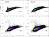 |
Fig. B.1 Same as Fig. 2, but for the GDS and using PSF photometry. |
| In the text | |
|
Fig. B.2 Colour-colour diagram of the stars located at field SPLUS-d288 of the GDS, similar to those found in Fig. 3. The red lines represent the original fit to all data, while the black dashed lines represent the final fits to the upper locus of points, obtained by applying an iterative fitting process to the initial fit. |
| In the text | |
|
Fig. C.1 Distribution of RR Lyrae stars from the catalogue of Greer et al. (2017) matched with S-PLUS data, shown in the (r – J0660) vs (r – i) diagram. The horizontal dashed line indicates the (r – J0660) = 0 value. |
| In the text | |
|
Fig. C.2 Distribution of Hα excess objects in Galactic longitude and latitude coordinates. The upper panel shows all the Hα sources selected, and the lower panel is a zoomed-in view of their distribution in the GDS. |
| In the text | |
Current usage metrics show cumulative count of Article Views (full-text article views including HTML views, PDF and ePub downloads, according to the available data) and Abstracts Views on Vision4Press platform.
Data correspond to usage on the plateform after 2015. The current usage metrics is available 48-96 hours after online publication and is updated daily on week days.
Initial download of the metrics may take a while.