| Issue |
A&A
Volume 695, March 2025
|
|
|---|---|---|
| Article Number | A281 | |
| Number of page(s) | 25 | |
| Section | Planets, planetary systems, and small bodies | |
| DOI | https://doi.org/10.1051/0004-6361/202452916 | |
| Published online | 03 April 2025 | |
TOI-2015 b: A sub-Neptune in strong gravitational interaction with an outer non-transiting planet
1
Astrobiology Research Unit, Université de Liège,
Allée du 6 Août 19C,
4000
Liège,
Belgium
2
Department of Earth, Atmospheric and Planetary Science, Massachusetts Institute of Technology,
77 Massachusetts Avenue,
Cambridge,
MA
02139,
USA
3
Instituto de Astrofísica de Canarias (IAC), Calle Vía Láctea s/n,
38200,
La Laguna, Tenerife,
Spain
4
Lund Observatory, Division of Astrophysics, Department of Physics, Lund University,
Box 118,
22100
Lund,
Sweden
5
Department of Earth Sciences, University of Hawaii at Manoa,
1680 East-West Rd,
Honolulu,
HI
96822,
USA
6
Institute for Astrophysics, University of Vienna,
Türkenschanzstrasse 17,
1180
Vienna,
Austria
7
Department of Astronomy and Astrobiology Program, University of Washington,
Box 351580,
Seattle, Washington
98195,
USA
8
NExSS Virtual Planetary Laboratory,
Box 351580, University of Washington,
Seattle, Washington
98195,
USA
9
Departamento de Astrofísica, Universidad de La Laguna (ULL),
E-38206
La Laguna, Tenerife,
Spain
10
Instituto de Astrofísica de Andalucía (IAA-CSIC), Glorieta de la Astronomía s/n,
18008
Granada,
Spain
11
INAF- Palermo Astronomical Observatory,
Piazza del Parlamento, 1,
90134
Palermo,
Italy
12
Komaba Institute for Science, The University of Tokyo,
3-8-1 Komaba, Meguro,
Tokyo
153-8902,
Japan
13
Astrobiology Center,
2-21-1 Osawa, Mitaka,
Tokyo
181-8588,
Japan
14
Research Institute for Advanced Computer Science, Universities Space Research Association,
Washington,
DC
20024,
USA
15
Institute for Particle Physics and Astrophysics, ETH Zürich,
OttoStern-Weg 5,
8093
Zürich,
Switzerland
16
Department of Astrophysics, University of Zürich, Winterthurerstrasse
190 8057
Zürich,
Switzerland
17
Department of Astronomy & Astrophysics, University of Chicago,
Chicago,
IL,
USA
18
Department of Physics and Kavli Institute for Astrophysics and Space Research, Massachusetts Institute of Technology,
Cambridge,
MA
02139,
USA
19
Space Sciences, Technologies and Astrophysics Research (STAR) Institute, Université de Liège,
Allée du 6 Août 19C,
B-4000
Liège,
Belgium
20
Instituto de Alta Investigación, Universidad de Tarapacá,
Casilla 7D,
Arica,
Chile
21
Gemini Observatory/NSF NOIRLab,
670 N. A’ohoku Place,
Hilo,
HI
96720,
USA
22
Departamento de Ingeniería Topográfica y Cartografía, E.T.S.I. en Topografía, Geodesia y Cartografía, Universidad Politécnica de Madrid,
28031
Madrid,
Spain
23
Subaru Telescope, National Astronomical Observatory of Japan,
650 North A‘ohoku Place,
Hilo,
HI
96720,
USA
24
Hamburger Sternwarte,
Gojenbergsweg 112,
21029
Hamburg,
Germany
25
Oukaimeden Observatory, High Energy Physics and Astrophysics Laboratory, Faculty of sciences Semlalia, Cadi Ayyad University,
Marrakech,
Morocco
26
Center for Astrophysics | Harvard & Smithsonian,
60 Garden Street,
Cambridge,
MA
02138,
USA
27
Kavli Institute for Particle Astrophysics & Cosmology, Stanford University,
Stanford,
CA
94305,
USA
28
Department of Astronomy, California Institute of Technology,
Pasadena,
CA
91125,
USA
29
Department of Astronomy & Space Sciences, Faculty of Science, Ankara University,
06100
Ankara,
Türkiye
30
Ankara University, Astronomy and Space Sciences Research and Application Center (Kreiken Observatory),
Incek Blvd.,
06837
Ahlatlıbel, Ankara,
Türkiye
31
AIM, CEA, CNRS, Université Paris-Saclay, Université de Paris,
91191
Gif-sur-Yvette,
France
32
School of Physics & Astronomy, University of Birmingham, Edgbaston,
Birmingham
B15 2TT,
UK
33
Center for Astrophysics and Space Sciences, UC San Diego,
UCSD Mail Code 0424, 9500 Gilman Drive,
La Jolla,
CA
92093-0424,
USA
34
American Association of Variable Star Observers,
185 Alewife Brook Parkway, Suite 410,
Cambridge,
MA
02138,
USA
35
George Mason University,
4400 University Drive,
Fairfax,
VA
22030,
USA
36
Department of Astronomy, University of California Berkeley,
Berkeley,
CA
94720,
USA
37
Department of Multi-Disciplinary Sciences, Graduate School of Arts and Sciences, The University of Tokyo,
3-8-1 Komaba, Meguro,
Tokyo
153-8902,
Japan
38
Dpto. Física Teórica y del Cosmos, Universidad de Granada,
18071
Granada,
Spain
39
Center for Space and Habitability, University of Bern,
Gesellschaftsstrasse 6,
3012
Bern,
Switzerland
40
Center for Computational Astrophysics, Flatiron Institute,
162 Fifth Avenue,
New York,
NY
10010,
USA
41
Universidad Nacional Autónoma de México, Instituto de Astronomía,
AP 70-264,
Ciudad de México
04510,
Mexico
42
European Space Agency (ESA), European Space Research and Technology Centre (ESTEC),
Keplerlaan 1,
2201
AZ
Noordwijk,
The Netherlands
43
SUPA Physics and Astronomy, University of St. Andrews, Fife,
KY16 9SS
Scotland,
UK
44
Cavendish Laboratory,
JJ Thomson Avenue,
Cambridge
CB3 0HE,
UK
45
Center for Interdisciplinary Exploration and Research in Astrophysics (CIERA), Northwestern University,
1800 Sherman,
Evanston,
IL
60201,
USA
46
Okayama Observatory, Kyoto University,
3037-5 Honjo, Kamogatacho, Asakuchi,
Okayama
719-0232,
Japan
47
NASA Ames Research Center,
Moffett Field,
CA
94035,
USA
48
Department of Physical Sciences, Ritsumeikan University, Kusatsu,
Shiga
525-8577,
Japan
49
Department of Physics and Astronomy, University of Louisville,
Louisville,
KY
40292,
USA
50
Freie Universität Berlin, Institute of Geological Sciences,
Malteserstr. 74-100,
12249
Berlin,
Germany
51
Sabadell Astronomical Society,
08206
Sabadell, Barcelona,
Spain
52
Europlanet Society, Department of Planetary Atmospheres of the Royal Belgian Institute for Space Aeronomy,
B-1180
Brussels,
Belgium
53
National Astronomical Observatory of Japan,
2-21-1 Osawa, Mitaka,
Tokyo
181-8588,
Japan
54
Astronomical Science Program, Graduate University for Advanced Studies,
SOKENDAI, 2-21-1, Osawa, Mitaka,
Tokyo,
181-8588,
Japan
55
Department of Physics, University of Rome “Tor Vergata”,
Via della Ricerca Scientifica 1,
00133,
Rome,
Italy
56
INAF – Astrophysical Observatory of Turin,
via Osservatorio 20,
10025,
Pino Torinese,
Italy
57
Max Planck Institute for Astronomy,
Königstuhl 17,
69117,
Heidelberg,
Germany
58
Villa ’39 Observatory,
Landers,
CA
92285,
USA
59
Wild Boar Remote Observatory, San Casciano in val di Pesa,
Firenze
50026,
Italy
60
Institute for Particle Physics and Astrophysics, ETH Zürich,
Wolfgang-Pauli-Strasse 2,
8093
Zürich,
Switzeland
61
Department of Physics, Aristotle University of Thessaloniki, University Campus,
Thessaloniki
54124,
Greece
62
Department of Astronomy, University of Maryland,
College Park,
College Park,
MD
20742,
USA
63
7 Skies Observatory, Cypress County, Alberta, RASC (Royal Astronomical Society of Canada),
Canada
64
South African Astronomical Observatory,
PO Box 9, Observatory,
Cape Town
7935,
South Africa
65
Astrophysics Group, Keele University,
Staffordshire
ST5 5BG,
UK
66
INAF – Osservatorio Astronomico di Padova,
Vicolo dell’Osservatorio 5,
35122
Padova,
Italy
67
Anton Pannekoek Institute for Astronomy, University of Amsterdam,
Science Park 904,
1098
XH
Amsterdam,
The Netherlands
68
Landessternwarte, Zentrum für Astronomie der Universität Heidelberg,
Königstuhl 12,
69117
Heidelberg,
Germany
69
Kotizarovci Observatory,
Sarsoni 90,
51216
Viskovo,
Croatia
70
Institute of Astronomy and Astrophysics, Academia Sinica,
PO Box 23-141, Taipei
10617,
Taiwan,
ROC
71
Department of Astrophysics, National Taiwan University, Taipei
10617,
Taiwan,
ROC
72
Department of Physics & Astronomy, Johns Hopkins University,
3400 N. Charles Street,
Baltimore,
MD
21218,
USA
73
Department of Physics and Astronomy, Union College,
807 Union St.,
Schenectady,
NY
12308,
USA
74
Department of Astrophysical Sciences, Princeton University,
Princeton,
NJ
08544,
USA
75
Department of Physics, Engineering and Astronomy, Stephen F. Austin State University,
1936 North St,
Nacogdoches,
TX
75962,
USA
★ Corresponding author; This email address is being protected from spambots. You need JavaScript enabled to view it.
Received:
7
November
2024
Accepted:
10
February
2025
Abstract
TOI-2015 is a known exoplanetary system around an M4 dwarf star, consisting of a transiting sub-Neptune planet in a 3.35-day orbital period, TOI-2015 b, accompanied by a non-transiting companion, TOI-2015 c. High-precision radial-velocity measurements were taken with the MAROON-X spectrograph, and high-precision photometric data were collected, primarily using the SPECULOOS, MUSCAT, TRAPPIST and LCOGT networks. We collected 63 transit light curves and 49 different transit epochs for TOI-2015 b. We recharacterized the target star by combining optical spectra obtained by the MAROON-X, Shane/KAST and IRTF/SpeX spectrographs, Bayesian model averaging (BMA) and spectral energy distribution (SED) analysis. The TOI-2015 host star is a K = 10.3 mag M4-type dwarf with a subsolar metallicity of [Fe/H] = −0.31 ± 0.16, and an effective temperature of Teff ≈ 3200 K. Our photodynamical analysis of the system strongly favors the 5:3 mean-motion resonance and in this scenario the planet b (TOI-2015 b) has an orbital period of Pb = 3.34 days, a mass of Mp = 9.02-0.36+0.32M⊕ , and a radius of Rp = 3.309-0.011+0.013R⊕ , resulting in a density of ρp = 0.25 ± 0.01 ρ⊕ = 1.40 ± 0.06 g cm−3; this is indicative of a Neptune-like composition. Its transits exhibit large (> 1 hr) timing variations characteristic of an outer perturber in the system. We performed a global analysis of the high-resolution radial-velocity measurements, the photometric data, and the TTVs, and inferred that TOI-2015 hosts a second planet, TOI-2015 c, in a non-transiting configuration. Our analysis places it near a 5:3 resonance with an orbital period of Pc = 5.583 days and a mass of Mp = 8.91-0.40+0.38M⊕. The dynamical configuration of TOI-2015 b and TOI-2015 c can be used to constrain the system’s planetary formation and migration history. Based on the mass-radius composition models, TOI-2015 b is a water-rich or rocky planet with a hydrogen-helium envelope. Moreover, TOI-2015 b has a high transmission-spectroscopic metric (TSM=149), making it a favorable target for future transmission spectroscopic observations with the JWST to constrain the atmospheric composition of the planet. Such observations would also help to break the degeneracies in theoretical models of the planet’s interior structure.
Key words: planets and satellites: detection / planets and satellites: formation / stars: individual: TOI-2015
Paris Region Fellow, Marie Sklodowska-Curie Action.
NHFP Sagan Fellow.
© The Authors 2025
 Open Access article, published by EDP Sciences, under the terms of the Creative Commons Attribution License (https://creativecommons.org/licenses/by/4.0), which permits unrestricted use, distribution, and reproduction in any medium, provided the original work is properly cited.
This article is published in open access under the Subscribe to Open model. This email address is being protected from spambots. You need JavaScript enabled to view it. to support open access publication.
1 Introduction
The Milky Way is dominated by M dwarf stars (Henry 1994; Henry et al. 2006), which are intriguing targets for searching for and characterizing small planets. M-dwarf systems offer a unique opportunity to explore their physical properties thanks to their small sizes and low masses. The relatively small size of the host star leads to deep transits, and large radial-velocity (RV) and TTV signals. This allowed us to explore the interior structure and atmospheric composition of the planets, by measuring their sizes and masses (e.g. Dorn et al. 2017).
Transit timing variations (TTVs, Agol et al. 2005; Holman & Murray 2005) can be used to search for additional non-transiting exoplanets and to estimate their physical parameters (orbital parameters and planetary masses) thanks to the planet’s gravitational perturbation. The TTV amplitude depends on the mass of the perturbing planet as well as the orbital eccentricities and longitudes of the pericenter of each planet (see, e.g., Deck & Agol 2016). Transiting planets in a multi-planet system with strong gravitational influences offer us an excellent opportunity to explore the interior composition of exoplanets. Moreover, the combination of planet sizes measured from transit depths and masses measured from TTVs and RVs yields densities and clues to the interior composition of planets. Near-resonant multi-planet systems, which exhibit nearly exact integer ratios of their orbital periods, offer special opportunities to derive the formation and evolution mechanisms of the systems. Currently, there are about 374 planetary systems that show TTVs, only ~20 of which orbit M dwarfs, including the well-characterized TRAPPIST-1 system, a resonant system with seven transiting rocky worlds orbiting a nearby late M-dwarf star (Gillon et al. 2016, 2017; Agol et al. 2021a).
TOI-2015 was confirmed by Jones et al. (2024) using the Transiting Exoplanet Survey Satellite data, and WIRO-2.3m, and RBO-0.6 m and ARC-3.5 m photometric data and RV measurements collected with the Habitable-zone Planet Finder Spectrograph. The analysis Jones et al. (2024) placed the non-transiting planet TOI-2015 c within near 2:1 resonance. The authors found that TOI-2015 b has a radius of ![Mathematical equation: $\[R_{b}=3.37_{-0.20}^{+0.15} R_{\oplus}\]$](/articles/aa/full_html/2025/03/aa52916-24/aa52916-24-eq4.png) and a mass of
and a mass of ![Mathematical equation: $\[M_{b}=13.3_{-4.5}^{+4.7} M_{\oplus}\]$](/articles/aa/full_html/2025/03/aa52916-24/aa52916-24-eq5.png) , and TOI-2015 c has a mass of
, and TOI-2015 c has a mass of ![Mathematical equation: $\[M_{c}= 6.8_{-2.3}^{+3.5} M_{\oplus}\]$](/articles/aa/full_html/2025/03/aa52916-24/aa52916-24-eq6.png) . However, other possible two-planet solutions –such as 3:2 and 4:3 near-resonances– could not be conclusively excluded without complementary photometric and RV observations. In this paper, we extended their analysis including further period ratios (5:3 and 5:2 resonances) to justify and set the stage for the justification for the paper. In this context, we present a new photodynamical analysis of the TOI-2015 system using TESS data, new ground-based photometric data and radial velocity measurements collected with the MAROON-X spectrograph. We collected a total of 63 transit light curves of the transiting planet TOI-2015 b and 28 radial velocity measurements. This enabled us to enhance the accuracy of the physical parameters of both planets, and better constrain composition and origin.
. However, other possible two-planet solutions –such as 3:2 and 4:3 near-resonances– could not be conclusively excluded without complementary photometric and RV observations. In this paper, we extended their analysis including further period ratios (5:3 and 5:2 resonances) to justify and set the stage for the justification for the paper. In this context, we present a new photodynamical analysis of the TOI-2015 system using TESS data, new ground-based photometric data and radial velocity measurements collected with the MAROON-X spectrograph. We collected a total of 63 transit light curves of the transiting planet TOI-2015 b and 28 radial velocity measurements. This enabled us to enhance the accuracy of the physical parameters of both planets, and better constrain composition and origin.
The paper is structured as follows. Section 2 describes the TESS and ground-based follow-up (photometric, spectroscopic, and high-angular-resolution imaging) observations used to characterize the system. Section 3 describes the stellar characterization of TOI-2015 using spectral energy distributions (SEDs), stellar evolution models, spectroscopic observations, and spectral and photometric fitting using Bayesian model averaging (BMA). The validation of the planet transit signals in the photometric data is presented in Section 4. A photodynamical analysis of photometric data, RVs, and TTV measurements is presented in Section 5, and an independent TTV analysis is presented in Section 6, allowing us to characterize the system. The planet searches and detection limits are presented in Section 7. Finally, our discussion and conclusions are presented in Sections 8 and 9, respectively.
2 Observation and data reduction
2.1 TESS photometry
The host star TIC 368287008 (TOI-2015) was observed by TESS (Ricker et al. 2015) in Sectors 24, 51, and 78 for 27 days each with 2-min cadence. Observation dates are presented in Table B.1. The Sector 51 campaign started on 2022 April 22 and ended on 2022 May 18. The two gaps during Sector 51 were caused by scattered light and high background levels1, and we ignored them. The Sector 78 campaign started on 2024 April 23 and ended on 2024 May 21. The target was observed in Camera 1 CCD 3. The first gap in the data is due to the Safe Hold mode of the spacecraft, while the second gap is due to the scattered light as Camera 1 was too close to Earth between BJDTDB = 2460444 and BJDTDB = 2460449 (see TESS observation report)2.
To analyze the TESS photometric data, we used the presearch data conditioning light curves (PCD-SAP) extracted from the Mikulski Archive for Space Telescopes (Stumpe et al. 2012; Smith et al. 2012; Stumpe et al. 2014) constructed by the TESS Science Processing Operations Center (SPOC, Jenkins et al. 2016) at Ames Research Center. PDC-SAP light curves have been corrected for any crowding and instrument systematics effects. The signature of TOI-2015 b was first detected by the TESS SPOC pipeline in Sectors 24 and 51. The TOI-2015 FOV including the location of nearby Gaia DR3 sources (Gaia Collaboration 2021) and photometric apertures are presented in Figure 1. TESS transit light curves for TOI-2015 b are presented in Figure 2.
2.2 Ground-based photometric follow-up
We used the TESS Transit Finder tool to schedule the photometric observations. It is a customized version of the Tapir software package (Jensen 2013). These are summarized in the following sections, and the resulting transit light curves are presented in Figure 3. The observation log is presented in Table C.1. The transit timing measurements are presented in Table D.1.
2.2.1 SPECULOOS-North
We used SPECULOOS-North/Artemis (Search for habitable Planets EClipsing ULtra-cOOl Stars, Burdanov et al. 2022) at Teide observatory to observe the transits of TOI-2015 b. Artemis is a 1.0-m Ritchey-Chrétien telescope equipped with a thermoelectrically cooled 2K×2K Andor iKon-L BEX2-DD CCD camera with a pixel scale of 0.35″/pixel and a total field-of-view (FOV) of 12′ × 12′. SPECULOOS-North is a sibling of the SPECULOOS-South (Jehin et al. 2018; Delrez et al. 2018; Sebastian et al. 2021) and SAINT-EX (Search And characterIsatioN of Transiting EXoplanets, Demory et al. 2020) telescopes. We observed a total of 15 (full and partial) transits in the I + z filter with an exposure time of 10s. The observation dates are presented in Table C.1. Data calibration and photometric extraction were performed using the PROSE3 pipeline (Garcia et al. 2022).
2.2.2 SAINT-EX
We observed one full transit of TOI-2015 b with SAINT-EX on UT 2022 June 19 in the I + z′ filter with an exposure time of 10 s. SAINT-EX (Demory et al. 2020) is a 1.0-m f/8 Ritchey-Chrétien telescope located at the Sierra de San Pedro Mártir in Baja California, México. SAINT-EX is equipped with a thermoelectrically cooled 2K×2K Andor iKon-L CCD camera, with a FOV of 12′×12′ and a pixel scale of 0.35″/pixel. The data calibration and photometric extraction were performed using the PROSE pipeline (Garcia et al. 2022).
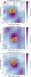 |
Fig. 1 TESS target pixel file images of TOI-2015 observed in Sectors 24 (top), 51 (middle), and 78 (bottom) made by tpfplotter (Aller et al. 2020). Red dots show the location of Gaia DR3 sources, and the yellow shaded regions show the photometric apertures used to extract the photometric measurements. |
2.2.3 TRAPPIST-South
One full transit was observed with the TRAPPIST-South (TRAnsiting Planets and PlanetesImals Small Telescope, Jehin et al. 2011; Gillon et al. 2011) telescope on UT 2022 May 29 in the I + z′ filter with an exposure time of 55 s. It is a 60-cm Ritchey-Chrétien telescope located at ESO-La Silla Observatory in Chile, which is the twin of TRAPPIST-North. It is equipped with a 2K×2K FLI Proline CCD camera with a FOV of 22′ × 22′ and a pixel scale of 0.65″/pixel. The data calibration and photometric extraction were performed using the PROSE pipeline (Garcia et al. 2022).
2.2.4 TRAPPIST-North
TRAPPIST-North (Barkaoui et al. 2019) observed three transits of TOI-2015 b in the I + z′ filter with an exposure time of 50s. The telescope is a 60-cm Ritchey-Chrétien telescope located at Oukaimeden Observatory, and it is equipped with a thermoelectrically cooled 2K×2K Andor iKon-L BEX2-DD CCD camera with a pixel scale of 0.6″, resulting in a FOV of 20′ × 20′. The data calibration and photometric extraction were performed using the PROSE pipeline (Garcia et al. 2022). The observation dates are given in Table C.1.
2.2.5 MuSCAT
We observed one full transit of TOI-2015 b on UT 2022 May 06 with MuSCAT, a simultaneous multi-band camera installed on the 188-cm telescope in Okayama, Japan (Narita et al. 2015). MuSCAT has three optical channels of g′, r′, and zs-bands with a pixel scale of 0.358″/pixel and 6′.1 × 6′.1 field of view. The reduction and the aperture photometry were conducted by the custom pipeline described in Fukui et al. (2011). The optimal aperture radius and set of comparison stars were selected for each band to minimize the scatter in the light curves.
2.2.6 MuSCAT2
Two full transits of TOI-2015b were observed on UT 2022 May 19 and 2022 May 29 with the MuSCAT2 multicolor imager (Narita et al. 2019) mounted on the 1.52 m-Telescopio Carlos Sánchez (TCS) at the Teide Observatory in Tenerife (Canary Islands, Spain). Both transits were carried out simultaneously in the Sloan-g, -r, -i, and zs. The photometric measurements were extracted using an uncontaminated photometric aperture (see Table C.1). The data calibration and photometric analysis were performed using the MuSCAT2 photometry pipeline (Parviainen et al. 2020).
2.2.7 LCOGT-2m0/MuSCAT3
We used the Las Cumbres Observatory Global Telescope (LCOGT; Brown et al. 2013) 2.0-m Faulkes Telescope North at Haleakala Observatory in Hawaii to observe a total of six transits of TOI-2015 b simultaneously in Sloan-g′, -r′, -i′, and zs filters. The observation dates are given in Table C.1. The telescope is equipped with the MuSCAT3 multiband imager (Narita et al. 2020). The data calibration was performed using the standard LCOGT BANZAI pipeline (McCully et al. 2018), and photometric measurements were extracted using AstroImage4 (Collins et al. 2017).
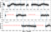 |
Fig. 2 TESS PDC-SAP flux extracted from 2-min cadence data of TOI-2015. The target was observed in Sectors 24 (top), 51 (middle), and 78 (bottom). The light gray points show the 2-min cadence data, and the black points show the flux in 30-min bins. The transit locations of TOI-2015 b are shown with vertical blue lines. |
2.2.8 LCOGT-1.0-m
We used the Las Cumbres Observatory Global Telescope (LCOGT; Brown et al. 2013) 1.0-m network to observe a total of 15 transits (full and partial) of TOI-2015 b in the Sloan-i′ filter. The observation dates are given in Table C.1. Each telescope is equipped with 4096×4096 SINISTRO Cameras, with an image scale of 0.389″ per pixel and a total FOV of 26′ × 26′. The data calibration was performed using the standard LCOGT BANZAI pipeline (McCully et al. 2018) and photometric measurements were extracted using AstroImageJ (Collins et al. 2017).
2.2.9 OSN-1.5m
We observed one partial transit of TOI-2015b on UT 2022 June 25 in the Johnson-Cousin I filter using the T150 at the Sierra Nevada Observatory in Granada (Spain). The T150 is equipped with a 2K×2K Andor iKon-L BEX2DD CCD camera with a pixel scale of 0.232″, resulting in a FOV of 7.9′×7.9′. The data calibration and photometric extraction were performed using AstroImageJ (Collins et al. 2017).
2.2.10 IAC80
We observed a full transit of TOI-2015 b on UT 2024 May 09 in the Sloan-r′ filter using the IAC80 telescope located at Teide Observatory in Tenerife (Canary Islands, Spain). The IAC80 is an 82 cm telescope equipped with a 4K×4K CCD camera with a plate scale of 0.32″/pixel, resulting in a FOV of 21.98′×22.06′. The data calibration and photometric extraction were performed using AstroImageJ (Collins et al. 2017).
2.2.11 T100
One full transit was observed with the 1-m Turkish telescope T100, located at the Türkiye National Observatories Bakırlıtepe Campus at an altitude of 2500 meters on UT 2023 June 25. The telescope is equipped with a cryo-cooled SI 1100 CCD that has 4096×4096 pixels, providing an effective field of view (FoV) of 21′ × 21′. We used the CCD in 2 × 2 binning mode to decrease the readout time from 45 s to 15 s. We slightly defocused the telescope to increase the precision (Bastürk et al. 2015) and observed without a filter, to capture all wavelengths of light and thus maximize the precision. Calibration of the raw images, aperture photometry with respect to an ensemble of comparison stars, and airmass detrending were performed using AstroImageJ.
2.2.12 CAHA-1.23 m
One full transit of TOI-2015 b was observed on UT 2023 June 15 with the Zeiss 1.23 m telescope at the Observatory of Calar Alto in Spain. The telescope is equipped with an iKon-XL 230 camera, with 4096 × 4108 pixels of size 15 μm. The pixel scale is 0.32 arcsec pixel−1 and the FOV is 21.4 arcmin × 21.5 arcmin. The transit was monitored through the special uncoated GG-495 glass long-pass filter (transparent at >500 nm). Observations were performed by slightly defocusing the telescopes, in order to increase the photometric precision (e.g., Southworth et al. 2012; Mancini et al. 2013), and using autoguiding. An exposure time between 110 and 120 seconds was adopted. The science data were calibrated by adopting the same procedure as in Mancini et al. (2017). Standard aperture photometry was used to extract the light curves of the planetary transit. This was done by placing the usual three apertures on the target and on five good comparison stars and running the APER routine (Southworth et al. 2010). The sizes of the apertures were decided after several attempts, by selecting those with the lowest scatter when compared with a fit model. The resulting light curve was normalized to zero magnitude by a quadratic fit to the out-of-transit data versus the comparison stars.
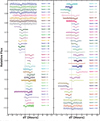 |
Fig. 3 TESS and ground-based transit light curves for TOI-2015 b, plotted with arbitrary vertical offsets for clarity. The colored data points show the relative flux and the black lines show the best-fitting transit model superimposed. The light curves are shifted along the x-axis according to the TTVs and along the y-axis for the visibility. The corresponding transit epoch is shown on the right of each transit light curve. |
2.3 Spectroscopy
2.3.1 Spectroscopic follow-up using MAROON-X
We observed TOI-2015 15 times with the MAROON-X spectrograph (Seifahrt et al. 2018, 2022) on Gemini-North between UT 2021 April and UT 2023 July. MAROON-X is an extreme precision radial velocity (EPRV) spectrograph with a wavelength coverage suitable for M-dwarf observations. MAROON-X has two CCDs encompassing different wavelength ranges, with a “red” channel at 650–920 nm and a “blue” channel at 500–670 nm. Both of these CCDs were exposed simultaneously during an observation of TOI-2015, meaning that we have 15 redchannel RVs and 15 blue-channel RVs. As these two channels are independent of one another and encompass different wavelength ranges, we consider them to be two different instruments for the purposes of our analysis, as they may capture different chromatic stellar signals.
The MAROON-X data were reduced using a custom Python3 pipeline and tools developed for the CRIRES instrument (Bean et al. 2010). We calculated RVs from the reduced spectrum using a modified version of serval (Zechmeister et al. 2020) customized to work with MAROON-X data. serval calculates RVs by co-adding all of the available spectra for the target to produce a high-S/R template, which is then compared to each individual spectrum in order to calculate the relative RV shift.
Our data have exposure times ranging from 520 to 1800 s, with one exposure at 2400 s. In general, we found that the spectra with 520 s exposure times had very large RV errors due to the faint nature of the host star. We increased our exposure times later in the survey in order to improve the RV precision (and reduce time lost to telescope overhead). Overall, we have ten exposures with the longer exposure times. Two of the short exposures in the blue channel had SNR < 10 and were thus not included in the serval results. Omitting the 520 s exposures, the red-channel spectra have a median SNR of 94 and a resulting median RV error of 1.4 m s−1. The blue-channel spectra have a median SNR of 33 and a median RV error of 3.1 m s−1. The resulting RV measurements and curve are presented in Table 1 and Figure 4.
2.3.2 IRTF/SpeX spectroscopy
We collected a medium-resolution near-infrared spectrum of TOI-2015 with the SpeX spectrograph (Rayner et al. 2003) on the 3.2-m NASA Infrared Telescope Facility (IRTF) on UT 2022 April 19. Thin cirrus was present, and seeing was ![Mathematical equation: $\[1^{\prime\prime}_\cdot0\]$](/articles/aa/full_html/2025/03/aa52916-24/aa52916-24-eq7.png) . Using the short-wavelength cross-dispersed (SXD) mode with the 0.3″ × 15″ slit aligned to the parallactic angle, we gathered spectra covering 0.80–2.42 μm with a resolving power of R~2000. Nodding in an ABBA pattern, we collected six exposures of 114.9 s each, totaling 689.4 s on source. We collected a standard set of SXD flat-field and arc-lamp exposures after the science observations, followed by a set of six, 3.7-s exposures of the A0 V star HD 140729 (V = 6.1). Data calibration was performed using Spextool v4.1 (Cushing et al. 2004), following the instructions for standard usage in the Spextool user manual5. The final spectrum has a median S/R per pixel of 83 with peaks in the J, H, and K bands of 108, 119, and 110, respectively, and an average of 2.7 pixels per resolution element.
. Using the short-wavelength cross-dispersed (SXD) mode with the 0.3″ × 15″ slit aligned to the parallactic angle, we gathered spectra covering 0.80–2.42 μm with a resolving power of R~2000. Nodding in an ABBA pattern, we collected six exposures of 114.9 s each, totaling 689.4 s on source. We collected a standard set of SXD flat-field and arc-lamp exposures after the science observations, followed by a set of six, 3.7-s exposures of the A0 V star HD 140729 (V = 6.1). Data calibration was performed using Spextool v4.1 (Cushing et al. 2004), following the instructions for standard usage in the Spextool user manual5. The final spectrum has a median S/R per pixel of 83 with peaks in the J, H, and K bands of 108, 119, and 110, respectively, and an average of 2.7 pixels per resolution element.
Radial-velocity measurements for TOI-2015 obtained by MAROON-X in the “red” and “blue” channels.
2.3.3 Shane/Kast optical spectroscopy
We observed TOI-2015 with the Kast double spectrograph (Miller & Stone 1994) mounted on the 3 m Shane telescope at Lick Observatory on UT 2022 July 02. Conditions were mostly clear with scattered clouds and 1″ seeing. We used the 1″ slit aligned to the parallactic angle to obtain blue and red optical spectra split at 5700 Å by the d 57 dichroic and dispersed by the 600/4310 grism and 600/7500 grating, respectively, for a common resolution of λ/Δλ ≈ 2000. We obtained a single 1200 s exposure in the blue channel and two 600 s exposures in the red channel at an average airmass of 1.07. The G2 V star HD 104385 (V = 8.57) was observed immediately before TOI-2015 for telluric absorption calibration, and the spectrophotometric calibrator Feige 66 (Hamuy et al. 1992, 1994) was observed during the night for flux calibration. We obtained HeHgCd and HeN eArHg arc lamp exposures at the start of the night to wavelength calibrate our blue and red data, respectively; flat-field lamp exposures for pixel-response calibration were also obtained. Data were reduced using the kastredux code6 using standard settings. We focused on our analysis on the higher quality red optical data which span 6000–9000 Å and have a median signal-to-noise ratio = 130 at 7350 Å.
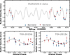 |
Fig. 4 Radial-velocity measurements in “red” (red triangles) and “blue” (blue triangles) channels with error bars) of the two-planets TOI-2015 b and TOI-2015 c collected with the MAROON-X spectrograph. The solid gray line shows the best-fit radial velocity data for the 5:3 scenario. |
2.4 High-resolution imaging
High-angular-resolution imaging is required to check for nearby sources that could contaminate the TESS photometry, resulting in an underestimated radius of the occulting object, or that can be the source of astrophysical false positives, such as blended eclipsing binaries.
2.4.1 4.1-m SOAR observations of TOI-2015
We searched for stellar companions to TOI-2015 using speckle imaging installed on the 4.1 m Southern Astrophysical Research (SOAR) telescope (Tokovinin 2018) on UT 2021 April 25, observing in the Cousins-I filter, a similar bandpass to TESS. This observation was sensitive enough to detect a 4.2-mag fainter star at an angular distance of 1 arcsec from the target. Further details of the SOAR observations are available in Ziegler et al. (2020). Figure 5 shows the speckle auto-correlation functions and the 5σ detection sensitivity. No nearby sources have been detected within 3″ of TOI-2015 in the SOAR data.
2.4.2 3.0 m-Shane observations of TOI-2015
We observed TOI-2015 with the ShARCS camera on the Shane 3.0-m telescope located at Lick Observatory (Kupke et al. 2012; Gavel et al. 2014; McGurk et al. 2014) on UT 2021 March 04. Observations were taken with the Shane adaptive optics system in natural-guide-star mode to search for nearby unresolved stellar companions. Sequences of observations were collected using the Ks and J filters. The data reduction was performed using the publicly available SImMER7 pipeline (Savel et al. 2020, 2022). No nearby stellar sources have been detected within detection limits (see Figure 5).
3 Stellar characterization
3.1 SED analysis and evolutionary models
As a first determination of the basic stellar parameters, we performed an analysis of the broadband SED of the star together with the Gaia DR3 parallax (with no systematic offset applied; see, e.g., Stassun & Torres 2021), in order to derive an empirical measurement of the stellar radius, following the procedures described in Stassun & Torres (2016); Stassun et al. (2017, 2018a). We pulled the J H KS magnitudes from 2MASS, the W1–W3 magnitudes from WISE, the GBPGRP magnitudes from Gaia, and the zy magnitudes from Pan-STARRS. Together, the available photometry spans the full stellar SED over the 0.4–10 μm wavelength range (see Figure 6).
We performed a fit using NextGen stellar atmosphere models, with the free parameters being the effective temperature (Teff) and metallicity ([Fe/H]); for the latter we adopted the spectroscopically determined value using MAROON-X data. In addition, we fixed the extinction AV ≡ 0 due to the proximity of the system to Earth. The resulting fit (Figure 6) has a best-fit Teff = 3200 ± 75 K, with a reduced χ2 of 1.3. Integrating the model SED gives the bolometric flux at Earth, Fbol = 1.552 ± 0.018 × 10⁻¹⁰ erg s−1 cm−2, which with the Gaia parallax gives the luminosity, Lbol = 0.010837 ± 0.000063 L⊙. Taking the Lbol and Teff together gives the stellar radius, R⋆ = 0.339 ± 0.016 R⊙. In addition, we derived the stellar mass from the empirical MK relations of Mann et al. (2019), giving M⋆ = 0.33 ± 0.02 M⊙.
We also checked stellar parameters as obtained from evolutionary modeling using CLES models for low-mass stars (Scuflaire et al. 2008; Fernandes et al. 2019). We used the luminosity derived just above, the metallicity [Fe/H]= −0.31 ± 0.16 from MAROON-X, and an assumed an age > 1 Gyr as inputs. We derived M⋆ = 0.28 ± 0.06 M⊙, within 1-σ agreement with the stellar mass found above. Other stellar parameters (stellar radius, effective temperature, etc.) are also found to be within 1 σ of the values derived above.
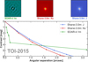 |
Fig. 5 High-angular-resolution imaging of TOI-2015 from 4.1-m SOAR telescope on UT 2021 April 25 in the Ks filter (green panel) and the 3.0-m SHANE telescope on UT 2021 March 04 in the K (red panel) and J (blue panel) bands. No stellar companions were found within detection limits. |
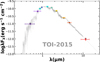 |
Fig. 6 Spectral Energy Distribution (SED) fit of TOI-2015. The gray curve is the best-fitting NextGen atmosphere model, the black circles show the model fluxes, while the colored circles with error bars show the observed fluxes. |
3.2 Spectroscopic analysis
We determined stellar parameters from the red part of the MAROON-X spectrum (see Figure 7) following the method described in Passegger et al. (2020) using the PHOENIX-ACES model grid (Husser et al. 2013) and assuming a stellar age of 5 Gyr for the evolutionary models (PARSEC, Bressan et al. (2012); Chen et al. (2014, 2015); Tang et al. 2014). With this, we derive parameters of Teff = 3211 ± 51 K, log g⋆ = 5.04 ± 0.04, and [Fe/H]= −0.31 ± 0.16. The derived metallicity of [Fe/H] = −0.31 ± 0.16 is significantly different from the values determined from SpeX and Kast spectra. We note that these spectrographs have lower spectral resolutions, and therefore different determination techniques have been used. As shown by Passegger et al. (2022), who compared different stellar parameter determination techniques, significant differences in the metallicity can be found by different methods, even when used on the same high-resolution spectra.
An independent analysis run with the same methods as Brady et al. (2024) recovered similar values for Teff (3237 ± 82 K) and [Fe/H] (−0.22 ± 0.16), which makes sense as both techniques utilize comparisons to PHOENIX model spectra to recover the stellar parameters. However, we note that the Brady et al. (2024) technique tends to perform unreliably for M dwarfs cooler than 3200 K, and the recovered temperature for TOI-2015 falls very close to this limit.
We also followed methods similar to those in Brady et al. (2024) to estimate the stellar v sin i by comparing the width of its cross-correlation function with an artificially broadened MAROON-X spectrum of Barnard’s Star, which, as an M4 star (Kirkpatrick et al. 1991), has a similar spectral type to TOI-2015. Overall, we recovered a v sin i value of 2.1 ± 0.4 km s−1. However, we note that, due to MAROON-X’s resolution, this method cannot measure vsini values lower than 2 km s−1, meaning that it is possible that TOI-2015 is rotating more slowly than the detection limit of MAROON-X. This value implies that TOI-2015 may be rotating more slowly than the v sin i = 3.2 ± 0.6 km s−1 quoted in Jones et al. (2024), which was close to the resolution limit of HPF. This discrepancy can be explained by the fact that MAROON-X has a higher resolution than HPF, allowing it to probe longer rotation periods. To be conservative, we thus quote a 2 σ upper limit of v sin i < 2.9 km s−1 for TOI-2015 from the MAROON-X data. This is in agreement with the 8.7 d photometric rotation period quoted by Jones et al. (2024), which predicts a v sin i ≲ 2 km s−1.
Figure 8 shows the SpeX SXD spectrum of TOI-2015. We used the SpeX Prism Library Analysis Toolkit (SPLAT, Burgasser & Splat Development Team 2017) to compare the spectrum to those of SpeX Prism standards (Kirkpatrick et al. 2010). We found the best spectral match to be the M4 standard Ross 47 (Gl 213), and we adopted an infrared spectral type of M4.0±0.5 for TOI-2015. Using SPLAT, we measured the equivalent widths of the K-band Na I and Ca I doublets and the H2O–K2 index (Rojas-Ayala et al. 2012). Following the Mann et al. (2013) relation between these observables and stellar metallicity, and propagating uncertainties using a Monte Carlo approach (see Delrez et al. 2022), we estimated an iron abundance of [Fe/H]= +0.29 ± 0.13.
Figure 9 compares the reduced Shane/Kast red optical spectrum of TOI-2015 to the M3, M4, and M5 dwarf spectral templates from Bochanski et al. (2007). The spectral morphology of TOI-2015 is intermediate between the M4 and M5 templates, suggesting an M4.5±0.5 optical classification, consistent with the near-infrared type. Both template-based classifications are also consistent with optical index-based classifications from Reid et al. (1995); Gizis (1997); Martín et al. (1999); Lépine et al. (2003); and Riddick et al. (2007), which span M3.5-M4.5. We detected strong Hα emission at 6563 Å with an equivalent width of −3.09 ± 0.08 Å, corresponding to log (LHα/Lbol) = −4.02 ± 0.06 using the χ factor relation of Douglas et al. (2014). This strong emission implies an activity age of no more than 5–6 Gyr (West et al. 2008), while the absence of detectable Li I absorption at 6708 Å rules out an age younger than ~30 Myr. We measured the metallicity index ζ = 1.057 ± 0.002 (Lépine et al. 2013) which corresponds to a slightly super-solar metallicity of [Fe/H]= 0.08 ± 0.20 using the Mann et al. (2013) calibration. This is formally consistent with the super-solar metallicity inferred from the SpeX data.
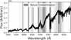 |
Fig. 7 MAROON-X spectrum of TOI-2015. The spectrum of TOI-2015 is shown in black. The gray regions are regions with telluric features in the spectrum, with darker gray indicating more tellurics. |
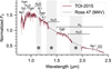 |
Fig. 8 SpeX SXD spectrum of TOI-2015. The spectrum of TOI-2015 is shown in red, and the SpeX Prism spectrum of the M4 standard Ross 47 is shown in gray for comparison. Strong spectral features of M dwarfs are indicated, and regions of high telluric absorption are shaded. |
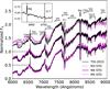 |
Fig. 9 Normalized Shane/Kast optical spectrum of TOI-2015 (black lines) compared to three SDSS spectral templates from Bochanski et al. (2007, magenta lines). Characteristic spectral features of mid-type M dwarfs are labeled. The inset box shows the 6520–6770 Å region encompassing Hα (in emission) and Li I (not detected). |
3.3 Spectral and photometric fitting using Bayesian model averaging
The SpeX SXD spectrum of TOI-2015, alongside photometric data from 2MASS (J H KS), ALLWISE (W1, W2), and Gaia DR3 (G, GRP), was used for a SED fit using four synthetic spectral model grids. The SpeX SXD spectrum was convolved to a wave-length resolution of R = 200 to ensure consistent analysis across the different grids. Absolute flux calibration was achieved by scaling the optical part of the SpeX SXD spectrum to match the Gaia XP spectrum (Gaia Collaboration 2023). For the spectral and photometric fitting, we employed four synthetic spectral libraries specifically designed to model the M dwarf regime: BT-Settl CIFIST (Allard et al. 2013), BT-Settl AGSS (Allard et al. 2012), Phoenix ACES (Husser et al. 2013), and SPHINX (Iyer et al. 2023). These libraries offer theoretical spectra and atmospheric models that account for various physical conditions in M dwarfs, making them appropriate for this analysis. The fitting process was carried out using the species toolkit (Stolker et al. 2020), which incorporates the nested sampling algorithm from the UltraNest package (Buchner 2023) to efficiently explore parameter space and estimate posterior distributions as well as Bayesian evidence. We adopted empirical relations for the Teff, radius, and mass of M dwarfs from Mann et al. (2015) as priors in this analysis, using Gaia DR3 magnitudes, parallax, and 2MASS Ks magnitude as constraints. The model grids cover [Fe/H] from −1.0 to +0.5 dex. A flat prior was used for extinction (Av), with potential values constrained between 0 and 0.2, given the star’s proximity. The parameters fit included Teff, [Fe/H], log g⋆, parallax, radius, and extinction. The carbon-to-oxygen (C/O) ratio was also fit for the SPHINX library without any prior. Furthermore, stellar-mass and luminosity estimates were derived from relations involving log g⋆, radius, parallax, and Teff.
We applied a BMA approach to combine the posterior distributions from each synthetic library. This method provides a robust estimation of stellar parameters by accounting for uncertainties between different models, yielding our final estimates for Teff, [Fe/H], log g⋆, parallax, radius, extinction, and, in the case of SPHINX, the C/O ratio. The best-fit synthetic spectrum and the residuals are shown in Figure 10, with the BMA values listed in Table 2. The final values obtained through BMA closely matched the best-fit results from the BT-Settl CIFIST library, since it is the grid with the most evidence. All grids provide a super-solar metallicity for TOI-2015, and the largest discrepancies in the posteriors distributions are found for Teff (median values from 3170 K to 3315 K), and therefore, for the stellar radius (median values from 0.3262 to 0.3548 R⊙).
4 Planet validation
4.1 TESS data validation
The SPOC performed a transit search of Sector 24 on 23 May 2020 (Jenkins 2002; Jenkins et al. 2010, 2020), which yielded a candidate with a 3.35 days period at a signal-to-noise ratio of S/N = 13.6. The TESS Science Office reviewed the vetting information and issued an alert on 2020 June 19 (Guerrero et al. 2021). The transit signal was also recovered in Sectors 51 and 78, and the transit signature passed all the diagnostic tests presented in the data-validation reports.
The transit depth found was 9753 ± 735 ppm, corresponding to a planet radius of 3.4 ± 0.4 R⊕ and a period of 3.34916 ± 0.00001 days. A comparison of the odd and even transit depths led to a 2-σ agreement. The target is quite isolated and no neighboring star was included in the TESS aperture (see Figure 1), although TOI-2015 was identified as the likely source of the events.
According to the difference image centroiding test (Twicken et al. 2018) for Sector 24, the host star is located within 5.058 ± 2.9 arcsec of the transit source. This result was then tightened up to 0.806 ± 3.0 arcsec in the sector 24–51 search. The transit source location is thus consistent with the host star.
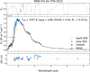 |
Fig. 10 Bayesian Model Averaging (BMA) fit for TOI-2015. The top panel shows the transmission curves of the filters considered, and the bottom panel displays the residuals. The observed SpeX SXD spectrum is shown in blue, while the black line represents the BT-Settl CIFIST synthetic spectrum using the BMA-derived stellar parameters, as shown in Table 1. The fluxes related to the photometry are shown by colors: orange for Gaia DR3, red for 2MASS, and purple for WISE. |
4.2 Ground-based photometric follow-up
We used the ground-based photometric observations to i) confirm the transit event on the target, ii) measure the transit timing variations and iii) check for the chromaticity for the transit depth in different wavelengths. Two of the closest neighboring stars to TOI-2015 are TIC 368287010 (Tmag = 12.97, ΔTmag = 0.18) at 33.3″ and TIC 368287012 (Tmag = 16.49, ΔTmag = 3.69) at 37.0″. We collected the observations in the I + z; Johnson-Ic; and Sloan-g′, -r′, -i′ and zs filters, covering a range from 400 to 1000 nm. This resulted in a non-chromatic dependence in different bands. The measured transit depths are presented in Figure 11.
4.3 Archival imaging
We used archival science images of TOI-2015 to exclude the background stellar objects that could be blended with our target in its current position. This kind of object might introduce the same transit event that we observed in our data and skew the physical properties of the system that we obtained from our photodynamical analysis. TOI-2015 has a relatively low proper motion of 64 mas/yr. We used images from POSS-II/DSS (Minkowski & Abell 1963) in 1952 in the blue filter and LCO-HAL-2m0/MuSCAT3 in 2024 in thezs filter, and they span 72 years. The target has moved by only 6.12″ from 1952 to 2024. There is no stellar background source at the present-day position of TOI-2015 (see Figure 12).
4.4 Statistical validation
We used the Tool for Rating Interesting Candidate Exoplanets and Reliability Analysis of Transits Originating from Proximate Stars (TRICERATOPS8, Giacalone et al. 2021) package to calculate the false positive probability, which allowed us to identify whether a given candidate is a planet or a nearby false positive. TRICERATOPS returns two parameters, which are the false positive probability (FPP) and the nearby false positive probability (NFPP). TRICERATOPS uses the phase-folded TESS light curves of the candidate and runs a Bayesian fit of several different possible astrophysical scenarios. It also allows us to implement high-contrast imaging observations in order to improve our results. In our case, we used the 4.1-m SOAR contrast curves described in Section 2.4. Using the TESS light curves of TOI-2015 b phase-folded on the orbital periods obtained from the photometric fit (see Section 5). Using ground-based observations (see Section 2.2), the transit event is detected on the target, and thus we excluded other nearby sources, which means that NFPP = 0 for TOI-2015 b. Typically, i) a given candidate is considered statistically validated when FPP<0.015 and NFPP<0.001, ii) a given candidate is likely a planet if FPP<0.5 and NFPP<0.001, and iii) a given candidate is a nearby false positive if NFPP>0.1. We ran TRICERATOPS using the TOI-2015 b phase-folded TESS light curves and the 4.1-m SOAR high contrast imaging observations. We obtained NFPP=0 and FPP= 0.0055 ± 0.0011. TOI-2015 b is validated planet.
Astrometry, photometry, and spectroscopy stellar properties of TOI-2015.
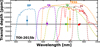 |
Fig. 11 Measured transit depths in different bands (colored dots with error bars) obtained in the global analysis for TOI-2015 b. The horizontal black line corresponds to the depth obtained from the achromatic fit with a 1σ error bar (shaded region). All measurements agree with the common transit depth at 1σ. Colored dashed lines show the transmission for each filter. |
5 Global modelling: Photometrics, TTVs, and RVs
We performed a set of photodynamical analyses modeling the TESS data, ground-based photometric observations, and the MAROON-X radial velocity measurements jointly using PyTTV (Korth et al. 2023; Korth et al. 2024). The code models the photometry and the radial velocities simultaneously using REBOUND (Rein & Liu 2012; Rein & Spiegel 2015; Tamayo et al. 2020) for dynamical integration and PyTransit (Parviainen 2015; Parviainen & Korth 2020; Parviainen 2020) for transit modeling, and provides posterior densities for the model parameters estimated using Markov chain Monte Carlo (MCMC) sampling in a standard Bayesian parameter estimation framework.
Table G.1 lists the model parameters and their priors. All planetary parameters, except for the log10 mass and radius ratio, are defined at a reference time of tref = 2459424.785 BJDTDB. We set uniform priors on the logarithmic masses of the two planets, with ranges designed to aid optimization without constraining the posteriors. For the inner planet’s radius ratio, we applied a loosely informative prior based on the visible transit depth, while the outer planet’s radius ratio is assigned a dummy normal prior, as the data cannot constrain it. We set a normal prior on the inner planet’s transit center and an uniform prior on the outer planet’s mean anomaly (the planets are parameterized differently since one transits and the other does not). A loosely informative prior is set on the inner planet’s impact parameter based on the transit fit, and a loosely informative normal prior is used for the outer planet’s impact parameter. We did not constrain the outer planet to non-transiting geometries because we are interested in seeing the preferred solutions without informing the analysis that the outer planet does not transit. Additionally, we set zero-centered half-normal priors on the eccentricities, 𝒩(0.0, 0.083), allowing for eccentric orbits while biasing against high eccentricities. Finally, we apply a normal prior on the stellar density, 𝒩(13, 1.3) g cm−3, based on stellar characterization.
Since the period of the second planet is unknown, we had to repeat the photodynamical analysis for all plausible period commensurability scenarios that could lead to the observed TTVs. We ignored the scenarios with an inner non-transiting planet and carried out analysis for scenarios where the other planet’s orbital period is close to the 2:1, 5:3, 5:2, 4:3 and 3:2 period commensurabilities. For each scenario, we set the prior for the outer planet’s period to 𝒩(r × 3.3491408, 0.02) days, where r is the period ratio corresponding to the scenario, and the 3.3491408 days period is derived from the linear ephemeris model.
The analysis starts with a global optimization using the differential evolution method (Storn 1997; Price et al. 2005) implemented in PyTransit (Parviainen 2015). The optimizer starts with a population of parameter vectors drawn from the model prior and clumps the population close to the global posterior mode. After the optimization, we used the clumped parameter vector population to initialize the emcee sampler (Foreman-Mackey et al. 2013), which we then used for MCMC sampling to obtain a sample from the parameter posterior. Finally, we tested the stability of the posterior solution by integrating a subset of posterior samples over 10000 years.
The best-fit solutions yield differential Bayesian information criterion (BIC – BIC5:3) values of 150, 0, −365, 517, and 183 for the 2:1, 5:3, 5:2, 4:3, and 3:2 scenarios, respectively. These results indicate that the BIC favors the 5:2 period commensurability scenario, with the 5:3 scenario emerging as the second-most preferred. However, stability tests reveal that the solutions for the 5:2 and 3:2 scenarios are unstable, leading to the ejection of one of the planets from the system within 10 000 years. Conversely, the solutions for the 2:1, 5:3, and 4:3 scenarios remain stable over the tested period. Among these, the 5:3 scenario is strongly favored over the 2:1 and 4:3 scenarios and also exhibits the smallest orbital inclination differences compared to the other configurations.
Adopting the 5:3 scenario, we find that TOI-2015 b is a sub-Neptune with a radius of ![Mathematical equation: $\[R_{p}=3.309_{-0.011}^{+0.013} R_{\oplus}\]$](/articles/aa/full_html/2025/03/aa52916-24/aa52916-24-eq13.png) , a mass of
, a mass of ![Mathematical equation: $\[M_{b}=9.20_{-0.36}^{+0.32} M_{\oplus}\]$](/articles/aa/full_html/2025/03/aa52916-24/aa52916-24-eq14.png) , and an eccentricity of
, and an eccentricity of ![Mathematical equation: $\[e_{b}=0.0789_{-0.0016}^{+0.0018}\]$](/articles/aa/full_html/2025/03/aa52916-24/aa52916-24-eq15.png) . The non-transiting planet, TOI-2015 c has a mass of
. The non-transiting planet, TOI-2015 c has a mass of ![Mathematical equation: $\[M_c== 9.52_{-0.36}^{+0.42} M_{\oplus}\]$](/articles/aa/full_html/2025/03/aa52916-24/aa52916-24-eq16.png) , an orbital period of Pc = 5.5829 days, and an eccentricity of
, an orbital period of Pc = 5.5829 days, and an eccentricity of ![Mathematical equation: $\[e_{c}=0.0004_{-0.0001}^{+0.0002}\]$](/articles/aa/full_html/2025/03/aa52916-24/aa52916-24-eq17.png) (see Table 3). Figure 13 shows the TTV data with fits for the 5:3 near-resonance scenario. We also present the results for the 2:1 and 5:2 scenarios in Tables E.1 and F.1.
(see Table 3). Figure 13 shows the TTV data with fits for the 5:3 near-resonance scenario. We also present the results for the 2:1 and 5:2 scenarios in Tables E.1 and F.1.
We also investigated the orbital stability of the 5:2, 5:3, and 2:1 MMR scenarios. To proceed, we extracted 200 configurations from each model posterior, and computed the dynamical evolution of the 3×200 configurations over 300 kyr. For these simulations, we used the WHFast integrator (Rein & Tamayo 2015) from the rebound software package (Rein & Liu 2012), with an integration timestep of ~1/70 Pb and a symplectic corrector of the order of 17. The number of system configurations that survived after 300 kyr (no escape, no close encounter) in the 5:2, 5:3, and 2:1 MMR scenarios are 159/200, 200/200, and 172/200, respectively. From these results, the 5:3 MMR scenario contains the largest number of stable configurations. Instead of the small orbital eccentricities, this higher stability rate is largely due to the low mutual inclination of this scenario. Indeed, we also ran simulations on the 5:2 MMR scenario with the hypothesis of co-planarity, and also obtained a higher stability rate. In conclusion, while the 5:3 MMR scenario is more plausible due to the larger number of stable systems, we cannot firmly exclude any of the other scenarios from pure orbital stability considerations.
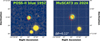 |
Fig. 12 Evolution of TOI-2015 position. The left panel shows an archival image of TOI-2015 taken using a photographic plate on the Palomar Schmidt Telescope in the blue filter. The right planet shows the zs image from LCO-HAL-2m0/MuSCAT3 taken in 2024. |
Physical parameters of TOI-2015 system for the 5:3 near-resonance scenario.
6 Independent analysis of TTV data
An independent analysis of the TTVs of the TOI-2015 b system was conducted using the transit-timing code NbodyGradient (Agol et al. 2021b). The fits were initialized near several MMR with period ratios near 4:3, 3:2, 5:3, 2:1 and 5:2. We found that each near-resonance gave fits to the transit times of similar quality, indicating that it is difficult to distinguish between these resonances based solely on transit-timing data, as found by Jones et al. (2024).
However, based on these fits, we find that the eccentricities are much lower in the 5:3 scenario than in the other cases (~0.01 vs ~0.1). In addition, we find that the masses in the 5:3 solution are very similar to those from our RV fit to the MAROON-X data with two-planets on circular orbits, indicating that this solution is, in fact, preferred over the others. The eccentricities in this fit are held to zero for convenience, but this turns out to be consistent with the low eccentricity found in the best-fit TTV model near the 5:3 period ratio.
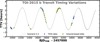 |
Fig. 13 Transit timing variation measurements for TOI-2015 b from TESS (blue points) and ground-based (green points) facilities. The gray line is the best-fit transit-timing model for the 5:3 scenario. |
7 Planet searches and detection limits from TESS
We processed the available 120 s TESS data using the SHERLOCK package (Pozuelos et al. 2020; Demory et al. 2020) to recover the original signal corresponding to TOI-2015 b detected by SPOC and search for other potential transiting planets that might remain unnoticed due to detection thresholds. We explored orbital periods from 0.5 to 25 d using ten detrended scenarios corresponding to window sizes ranging from 0.1 to 1.3 d; we refer the reader to Pozuelos et al. (2023) for further details about different searching strategies and to Dévora-Pajares et al. (2024) for a comprehensive update of all of SHERLOCK’s capabilities.
In the first run, we found the signal corresponding to the TOI-2015 b, which allowed us to confirm the detectability of this candidate independently. In the subsequent runs, SHERLOCK did not find any interesting detection, all the signals found being attributable to either intrinsic noise in the light curve not fully decorrelated by our detrending or to spurious detections.
Once we explored the data in the search for extra transiting planets, and since we know that there is at least a second planet in the system, we wanted to establish detection limits with the current data set. To this end we employed the MATRIX package (see, e.g., Dévora-Pajares & Pozuelos 2022; Delrez et al. 2022), which injects synthetic planets into the data using a range of orbital periods, planetary radii, and orbital phases, and tries to recover them, mimicking the procedure conducted by SHERLOCK. The purpose of this analysis is to determine the range of planetary sizes and orbital periods that could be reliably detected in our data set. In particular, we generated 6000 scenarios with the orbital period ranging from 0.5 to 15 d with steps of 0.5 d, and radii from 1 to 5 R⊕ with steps of 0.2 R⊕. Each radius-period pair was evaluated at ten orbital phases. The results are shown in Figure 14. We found that the planet corresponding to TOI-2015 b falls in a region with a 100% recovery rate. Moreover, we found that any planet larger than 3.0 R⊕ would be easily detectable, with recovery rates higher than 70% at any orbital period explored in this study. In contrast, planets with radii below 1.5 R⊕ would be undetectable, with recovery rates lower than 20% in all cases. Planets with radii between 1.5 and 3.0 R⊕ represent the transition region with recovery rates from 50 to 100%, with the shorter orbital period being the easier one to detect and vice versa. While the favored solution from the global fit presented in Section 5 corresponds to the MMR 5:3 between planets TOI-2015 b, and c, still other solutions might be possible, such as 4:3, 3:2, 2:1 and 5:2 (see Section 6). We highlight all these possibilities in Figure 14, and we conclude that in all the cases, any transiting planet larger than 2.0 R⊕ should be easily detectable, while smaller transiting planets might remain undetected in the current data set, and hence we cannot entirely rule out the transiting nature of planet c.
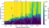 |
Fig. 14 Injection-and-recovery test performed to check the detectability of additional planets in the TOI-2015 system. We explored a total of 6000 different scenarios with the orbital period ranging from 0.5 to 15 days and radius from 1 to 5 R⊕. Larger recovery rates are presented in green and yellow, while lower recovery rates are shown in blue and darker hues. Planets larger than 3.0 R⊕ with P ≲ 10 d would be easily detectable. Planets below 1.5 R⊕ would be undetectable, with recovery rates lower than 20% in all cases. The dashed red lines show the MMR possibilities for the non-transiting planet. The blue dot refers to the planet TOI-2015 b. |
8 Discussion
8.1 Mass-radius and composition
Analyzing the observations from the TESS mission together with ground-based photometry and RV measurements collected with the MAROON-X spectrograph, we confirm the planetary nature of the transiting planet TOI-2015 b around its M4-dwarf host star. We find that the transiting planet TOI-2015 b has a radius and mass of ![Mathematical equation: $\[R_{p}=3.309_{-0.011}^{+0.013} R_{\oplus}\]$](/articles/aa/full_html/2025/03/aa52916-24/aa52916-24-eq41.png) and
and ![Mathematical equation: $\[M_{p}=9.20_{-0.36}^{+0.32} M_{\oplus}\]$](/articles/aa/full_html/2025/03/aa52916-24/aa52916-24-eq42.png) , respectively. This results in a mean density of
, respectively. This results in a mean density of ![Mathematical equation: $\[\rho_{p}=1.400_{-0.056}^{+0.052} \mathrm{~g} \mathrm{~cm}^{-3}\]$](/articles/aa/full_html/2025/03/aa52916-24/aa52916-24-eq43.png) , which is indicative of a Neptune-like composition. We present a comparative analysis of the mass and radius of TOI-2015 b with other transiting exoplanets, and composition models from Aguichine et al. (2021) and Lopez & Fortney (2014). The models of Aguichine et al. (2021) considered the mass-radius relation inferred from the water-rich composition models. These models assume a H2O-dominated atmosphere on top of a high-pressure water layer. We computed the mass-radius relationship from Aguichine et al. (2021) for different water fractions, and for a planetary equilibrium temperature of Teq = 500K (i.e. the equilibrium temperature closest to the one for TOI-2015 b). We assumed a core-mass fraction of xcore = 0.3 (i.e., Earth-like interior composition):
, which is indicative of a Neptune-like composition. We present a comparative analysis of the mass and radius of TOI-2015 b with other transiting exoplanets, and composition models from Aguichine et al. (2021) and Lopez & Fortney (2014). The models of Aguichine et al. (2021) considered the mass-radius relation inferred from the water-rich composition models. These models assume a H2O-dominated atmosphere on top of a high-pressure water layer. We computed the mass-radius relationship from Aguichine et al. (2021) for different water fractions, and for a planetary equilibrium temperature of Teq = 500K (i.e. the equilibrium temperature closest to the one for TOI-2015 b). We assumed a core-mass fraction of xcore = 0.3 (i.e., Earth-like interior composition):
![Mathematical equation: $\[\log _{10}\left(R_p\right)=a \log _{10}\left(M_p\right)+\exp \left[-d \times\left(\log _{10}\left(M_p\right)+c\right)\right]+b,\]$](/articles/aa/full_html/2025/03/aa52916-24/aa52916-24-eq44.png) (1)
(1)
where Rp is the planet radius in R⊕, Mp is the planet mass in M⊕, and a, b, c, and d are coefficients obtained by the Aguichine et al. (2021) fits. The results are shown in Figure 15 (solid colored lines). Based on this preliminary comparison, TOI-2015 b is compatible with a high water-mass fraction of 70%.
We also performed a similar analysis assuming a composition based on a rocky core surrounded by a hydrogen and helium envelope (Lopez & Fortney 2014). These models are generated for planets with masses from 1 to 20 M⊕, ages from 100 Myr to 10 Gyr, incident flux from 0.1 to 1000 F⊕, and envelope fractions from 0.01 to 20%. We used the tabulated mass-radius relations from the interior models of Lopez & Fortney (2014) for different hydrogen-helium (H2/He) fractions, assuming a planet incident flux of S p = 10 S⊕ (i.e., incident flux closest to the one for TOI-2015 b) and systems older than 1 Gyr. Figure 15 shows the mass-radius models (dashed colored lines). In this case, we find that the properties of TOI-2015 b are consistent with a gaseous envelope with a mass fraction of fenv ≈10% of the mass of the planet.
Our results show that models with water-rich and hydrogen-helium envelopes provide equally good matches to the planet density. A future measurement of the transmission spectrum of TOI-2015 b with the JWST might help break this degeneracy by providing a direct atmospheric composition of the upper layers of the outer envelope of the planet’s atmosphere.
8.2 Location in the period–radius diagram
Based on our photodynamical analysis of the system, TOI-2015 b has a period of Pb = 3.35 days. In Figure 16, we plotted the planet radius as a function of the orbital period of transiting exoplanets, along with the boundaries of the Neptune-desert. TOI-2015 b is located within a region between the “Neptune-desert” and “savanna”, defined as the “Neptunian-ridge” by Castro-González et al. (2024). This work suggests that the evolutionary mechanisms that bring planets to the Neptunian ridge might be similar to those that bring larger exoplanets to the hot-Jupiter (≃3–5 days) region. TOI-2015 b has a low eccentricity of ![Mathematical equation: $\[e_{b}=0.0770_{-0.0018}^{+0.0016}\]$](/articles/aa/full_html/2025/03/aa52916-24/aa52916-24-eq45.png) . This eccentricity is not high enough to start the HEM (high-eccentricity migration)(Fortney et al. 2021; Bourrier et al. 2023).
. This eccentricity is not high enough to start the HEM (high-eccentricity migration)(Fortney et al. 2021; Bourrier et al. 2023).
To account for the large-amplitude transit timing variations of TOI-2015 b, we identified an outer non-transiting companion likely to be in a 5:3 near-resonance motion, TOI-2015 c. Our TTV fit (Figure 13) implies an orbital period of ![Mathematical equation: $\[P_{c}= 5.582904_{-0.000043}^{+0.000044}\]$](/articles/aa/full_html/2025/03/aa52916-24/aa52916-24-eq46.png) days, a mass of
days, a mass of ![Mathematical equation: $\[M_{c}=8.91_{-0.40}^{+0.38} M_{\oplus}\]$](/articles/aa/full_html/2025/03/aa52916-24/aa52916-24-eq47.png) , and an eccentricity of
, and an eccentricity of ![Mathematical equation: $\[e_{c}=0.00033_{-0.0002}^{+0.0003}\]$](/articles/aa/full_html/2025/03/aa52916-24/aa52916-24-eq48.png) . The presence of this companion in the system might be partly responsible for inward migration of TOI-2015 b. The location of TOI-2015 b in the radius-period diagram (Figure 16), the presence of the companion, and future spin-orbit angle measurements will provide us with some more insights into the formation and evolution history of the system.
. The presence of this companion in the system might be partly responsible for inward migration of TOI-2015 b. The location of TOI-2015 b in the radius-period diagram (Figure 16), the presence of the companion, and future spin-orbit angle measurements will provide us with some more insights into the formation and evolution history of the system.
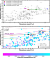 |
Fig. 15 Planetary radius as function of planetary mass of known transiting exoplanets well characterized, with radius and mass precisions better than 10% and 20%, respectively. Data are extracted from TEPCat (Southworth 2011). Top panel shows the comparison between the planetary parameters for TOI-2015 b. The red star shows our updated measurements, while the green dot with error bars shows the planetary parameters derived by Jones et al. (2024). We also highlighted the planetary parameters for other scenarios 2:1 (magenta square) and 5:2 (blue triangle). Bottom panel shows the comparison between TOI-2015 b to other transiting planetary systems. The systems are colored according to the stellar effective temperature. The size of the points is scaled according to the stellar radius. Dashed lines show the massradius composition models from Lopez & Fortney (2014). We display mass-radius curves for hydrogen-helium compositions of 5%, 10% and 20% H2/He. We assumed a planet with an incident flux of S p = 10 S⊕, and an age of > 1 Gyr. The solid lines present the mass-radius composition models from Aguichine et al. (2021). We display mass-radius curves for water-rich compositions of 70%, 90% and 100% H2O. We assumed a planetary equilibrium temperature of Teq = 500K and a core mass fraction of xcore = 0.3. We also highlighted the planetary parameters for other scenarios 2:1 (black square) and 5:2 (black triangle). Two Solar System planets (Uranus and Neptune) are also displayed. |
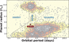 |
Fig. 16 Planetary radius versus orbital period diagram of known transiting exoplanets. Data are extracted from NASA Archive of Exoplanets. The location of the Neptunian desert, ridge, and savanna derived by Castro-González et al. (2024) are highlighted. TOI-2015 b is well placed in the Neptunian-ridge region. This plot is made using nep-des (https://github.com/castro-gzlz/nep-des). |
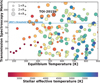 |
Fig. 17 Feasibility of TOI-2015 b for transmission spectroscopy studies. The transmission spectroscopy metric (TSM; Kempton et al. (2018)) as a function of the planetary equilibrium temperature of all known transiting exoplanets with mass measurement is shown. Data are extracted from the NASA Exoplanets Archive. The size of the points scales according to the planetary radius. The points are colored according to the stellar effective temperature. TOI-2015 b is highlighted by the black circle and error bars. |
8.3 Potential for atmospheric characterization for TOI-2015b
To quantify the suitability of transiting exoplanets for atmospheric characterization through transmission spectroscopy, we used the transmission spectroscopy metric (TSM) derived by Kempton et al. (2018). By combining the planetary radius, mass, equilibrium temperature, and the infrared stellar brightness, we find that TOI-2015 b has a TSM of 149.4 ± 5.6. Figure 17 plots the TSM as a function of the planetary equilibrium temperature for transiting exoplanets with mass measurements. This shows that TOI-2015 b is one of the best sub-Neptune planets for atmospheric exploration with the JWST.
We further explored the potential of TOI-2015 b for transmission spectroscopy with the JWST through spectral simulations for a suite of atmospheric scenarios. We adopted TauREx 3 (Al-Refaie et al. 2021) to simulate the synthetic transmission spectra. TOI-2015 b could retain an H/He-dominated and waterrich atmosphere (Sect 8.1). We modeled H/He atmospheres with 1× and 100× scaled solar abundances using the atmospheric chemical equilibrium module of Agúndez et al. (2012), including collision-induced absorption by H2−H2 and H2−He (Abel et al. 2011, 2012; Fletcher et al. 2018). For each chemical setup, we considered the cases of clear and hazy atmospheres. The haze was modeled using Mie scattering with the formalism of Lee et al. (2013), assuming the same haze parameters as in previous studies (Orell-Miquel et al. 2023; Goffo et al. 2024). We note that a super-solar metallicity is typically expected for sub-Neptune-sized planets (e.g., Fortney et al. 2013; Thorngren et al. 2016), while the planetary equilibrium temperature (Teq) within Teq ≈ 400–600 K also points to a high degree of haziness due to inefficient haze removal (Gao & Zhang 2020; Ohno & Tanaka 2021; Yu et al. 2021). Moreover, we modeled the case of a pure H2O atmosphere.
The ExoTETHyS (Morello et al. 2021) package has been used to simulate the corresponding JWST spectra with the NIRISSSOSS (λ =[0.6 μm-2.8 μm]), NIRSpec-G395H (λ =[2.88 μm–5.20 μm]), and MIRI-LRS (λ =[5 μm–12 μm]) instrumental modes. The ExoTETHyS code has been cross-validated against the Exoplanet Characterization Toolkit (ExoCTK, Bourque et al. 2021) and PandExo (Batalha et al. 2017) in a series of previous studies (Murgas et al. 2021; Espinoza et al. 2022; Luque et al. 2022a,b; Chaturvedi et al. 2022; Lillo-Box et al. 2023; Orell-Miquel et al. 2023; Palle et al. 2023; Goffo et al. 2024). We conservatively increased the uncertainty estimates by 20%. We considered wavelength bins with a spectral resolution of R ~100 for NIRISS and NIRSpec, and a constant bin size of 0.25 μm for MIRI-LRS observations, following the recommendations from recent JWST Early Release Science papers (Carter et al. 2024; Powell et al. 2024).
Figure 18 shows the synthetic transmission spectra for the atmospheric configurations described above. The H/He model atmospheres exhibit strong H2O and CH4 absorption features of ≳100–1000 ppm (parts per million), depending on metallicity and haze, while the steam H2O atmosphere has absorption features ≲100 ppm. The predicted error bars for a single transit observation are 60–273 ppm (mean error 110 ppm) for NIRISSSOSS, 86–256 ppm (mean error 123 ppm) for NIRSpec-G395H, and 125–190 ppm (mean error 144 ppm) for MIRI-LRS. Based on our simulations, a single transit observation with NIRSpecG395H or NIRISS-SOSS is well suited to detecting an H/He atmosphere, while at least four transit observations may be required to reveal features in the case of a steam atmosphere.
9 Conclusion
In this paper, we present a photodynamical analysis of the TOI-2015 exoplanetary system including the TESS and ground-based photometry, together with RV measurements obtained with the MAROON-X spectrograph (Section 2.3.1). To account for large-amplitude TTVs, the gravitational interaction between the planets is also included in our analysis. The host star is well characterized using optical and nearinfrared spectroscopic observations obtained by MAROON-X, Shane/KAST, and Magellan/FIRE spectrographs, together with SED (section 3.1), BMA (section 3.3), and stellar evolutionary models. The target was observed by the TESS mission in Sectors 24, 51, and 78 with a 2-min cadence. The intensive ground-based photometric observations were collected using SPECULOOS-North/Artemis-1m0, SAINT-EX-1m0, MuSCAT, MuSCAT2, LCOGT-2m0/MuSCAT3, LCOGT1 m 0, TRAPPIST-North/-South-0.6m, TUBITAK-1m0, IAC80, OSN-1.5m and CAHA-1.23m telescopes (Section 2.2). The photodynamical analysis was performed using the PyTTV pipeline developed by Korth et al. (2023); Korth et al. (2024) (Section 5), and an independent analysis (Section 6) was performed using the NbodyGradient code (Agol et al. 2021b). TOI-2015 is a K = 10.3 mag M4-type dwarf with a subsolar metallicity of [Fe/H] = −0.31 ± 0.16, an effective temperature of Teff = 3211 ± 51 K, and a surface gravity of log g⋆ = 5.04 ± 0.04 (cgs).
The TOI-2015 system is composed of two sub-Neptune exoplanets. The inner planet, TOI-2015 b is a transiting sub-Neptune at Pb = 3.35 days, with a radius of Rp = 3.31 ± 0.01 R⊕ and a mass of Mp = 9.86 ± 0.37 M⊕. To place TOI-2015 b in context within the exoplanet population, we plot the radius-mass diagram (Figure 15) for transit exoplanets with mass measurements. As a preliminary comparison, the planet has a degeneracy in its interior composition based on the mass-radius composition models from Lopez & Fortney (2014) and Aguichine et al. (2021). The measurement of a transmission spectrum from the JWST can help to break this degeneracy by providing the planet’s atmospheric composition.
The transit events of TOI-2015 b exhibit large TTVs indicative of an outer companion in the system, TOI-2015c. Our best-fit solution places the planet near a 5:3 resonance with an orbital period of Pc = 5.58 days, a mass of ![Mathematical equation: $\[M_{p}=9.20_{-0.35}^{+0.32} M_{\oplus}\]$](/articles/aa/full_html/2025/03/aa52916-24/aa52916-24-eq49.png) , and an eccentricity of
, and an eccentricity of ![Mathematical equation: $\[e_{b}=0.0789_{-0.0016}^{+0.0018}\]$](/articles/aa/full_html/2025/03/aa52916-24/aa52916-24-eq50.png) . Other scenarios for TOI-2015 c might be possible, such as the 2:1, 5:2, 3:2 and 4:3 resonances. More photometric data and RV measurements are required in order to break this degeneracy on the orbital period of TOI-2015 c.
. Other scenarios for TOI-2015 c might be possible, such as the 2:1, 5:2, 3:2 and 4:3 resonances. More photometric data and RV measurements are required in order to break this degeneracy on the orbital period of TOI-2015 c.
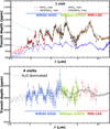 |
Fig. 18 Simulated synthetic atmospheric transmission spectra of TOI-2015 b. Top: fiducial models for clear or hazy H/He atmospheres with scaled solar abundances. Bottom: model for steam H2O atmosphere. Simulated measurements with error bars are shown for the observation of one (top) or four (bottom) transits with JWST NIRISS-SOSS, NIRSpec-G395H, and MIRI-LRS configurations. |
Data availability
The TESS photometric observations that we used in this work are available via the Mikulski Archive for Space Telescopes (MAST) and the ExoFOP-TESS platform. All ground-based photometric observations are also available via the ExoFOP-TESS platform. RV measurements collected with the MAROON-X spectrograph are available in Table 1.
Appendix A Acknowledgments
The postdoctoral fellowship of KB is funded by F.R.S.-FNRS grant T.0109.20 and by the Francqui Foundation. MG and EJ are F.R.S.-FNRS Research Directors. This publication benefits from the support of the French Community of Belgium in the context of the FRIA Doctoral Grant awarded to MT. Funding for the TESS mission is provided by NASA’s Science Mission Directorate. KAC and CNW acknowledge support from the TESS mission via subaward s3449 from MIT. This paper made use of data collected by the TESS mission, obtained from the Mikulski Archive for Space Telescopes MAST data archive at the Space Telescope Science Institute (STScI). Funding for the TESS mission is provided by the NASA Explorer Program. STScI is operated by the Association of Universities for Research in Astronomy, Inc., under NASA contract NAS 5–26555. We acknowledge the use of public TESS data from pipelines at the TESS Science Office and at the TESS Science Processing Operations Center. Resources supporting this work were provided by the NASA High-End Computing (HEC) Program through the NASA Advanced Supercomputing (NAS) Division at Ames Research Center for the production of the SPOC data products. This research has made use of the Exoplanet Follow-up Observation Program (ExoFOP; DOI: 10.26134/ExoFOP5) website, which is operated by the California Institute of Technology, under contract with the National Aeronautics and Space Administration under the Exoplanet Exploration Program. J.d.W. and MIT gratefully acknowledge financial support from the Heising-Simons Foundation, Dr. and Mrs. Colin Masson and Dr. Peter A. Gilman for Artemis, the first telescope of the SPECULOOS network situated in Tenerife, Spain. The ULiege’s contribution to SPECULOOS has received funding from the European Research Council under the European Union’s Seventh Framework Programme (FP/2007-2013) (grant Agreement n° 336480/SPECULOOS), from the Balzan Prize and Francqui Foundations, from the Belgian Scientific Research Foundation (F.R.S.-FNRS; grant n° T.0109.20), from the University of Liege, and from the ARC grant for Concerted Research Actions financed by the Wallonia-Brussels Federation. The research leading to these results has received funding from the ARC grant for Concerted Research Actions, financed by the Wallonia-Brussels Federation. TRAPPIST is funded by the Belgian Fund for Scientific Research (Fond National de la Recherche Scientifique, FNRS) under the grant PDR T.0120.21. TRAPPIST-North is a project funded by the University of Liege (Belgium), in collaboration with Cadi Ayyad University of Marrakech (Morocco). The ULiege’s contribution to SPECULOOS has received funding from the European Research Council under the European Union’s Seventh Framework Programme (FP/2007–2013) (grant Agreement n° 336480/SPECULOOS), from the Balzan Prize and Francqui Foundations, from the Belgian Scientific Research Foundation (F.R.S.-FNRS; grant n° T.0109.20), from the University of Liege, and from the ARC grant for Concerted Research Actions financed by the Wallonia-Brussels Federation. This work is supported by a grant from the Simons Foundation (PI Queloz, grant number 327127). J.d.W. and MIT gratefully acknowledge financial support from the Heising-Simons Foundation, Dr. and Mrs. Colin Masson and Dr. Peter A. Gilman for Artemis, the first telescope of the SPECULOOS network situated in Tenerife, Spain. This work is supported by the Swiss National Science Foundation (PP00P2-163967, PP00P2-190080 and the National Centre for Competence in Research PlanetS). This work has received fund from the European Research Council (ERC) under the European Union’s Horizon 2020 research and innovation programme (grant agreement n° 803193/BEBOP), from the MERAC foundation, and from the Science and Technology Facilities Council (STFC; grant n° ST/S00193X/1). This work is based upon observations carried out at the Observatorio Astronómico Nacional on the Sierra de San Pedro Mártir (OAN-SPM), Baja California, México. SAINT-EX observations and team were supported by the Swiss National Science Foundation (PP00P2163967 and PP00P2-190080), the Centre for Space and Habitability (CSH) of the University of Bern, the National Centre for Competence in Research PlanetS, supported by the Swiss National Science Foundation (SNSF). Author F.J.P, P.J.A, A.S. and A.P.T. acknowledge financial support from the Severo Ochoa grant CEX2021-001131-S funded by MCIN/AEI/10.13039/501100011033 and Ministerio de Ciencia e Innovación through the project PID2022-137241NB-C43. Partially based on observations made at the Observatorio de Sierra Nevada (OSN), operated by the Instituto de Astrofísica de Andalucía (IAA-CSIC). This work makes use of observations from the LCOGT network. Part of the LCOGT telescope time was granted by NOIRLab through the Mid-Scale Innovations Program (MSIP). MSIP is funded by NSF. This work is partly supported by JSPS KAKENHI Grant Number JP21K13955, JP24H00017, JP24H00248, JP24K00689, JP24K17082 and JP24K17083, JSPS Grant-in-Aid for JSPS Fellows Grant Number JP24KJ0241, Astrobiology Center SATELLITE Research project AB022006, JSPS Bilateral Program Number JPJSBP120249910 and JST SPRING, Grant Number JPMJSP2108. This article is based on observations made with the MuSCAT2 instrument, developed by ABC, at Telescopio Carlos Sánchez operated on the island of Tenerife by the IAC in the Spanish Observatorio del Teide. This paper is based on observations made with the MuSCAT3 instrument, developed by the Astrobiology Center and under financial supports by JSPS KAKENHI (JP18H05439) and JST PRESTO (JPMJPR1775), at Faulkes Telescope North on Maui, HI, operated by the Las Cumbres Observatory. We thank Türkiye National Observatories for the partial support in using T100 telescope with the project number 22BT100-1958. Visiting Astronomer at the Infrared Telescope Facility, which is operated by the University of Hawaii under contract 80HQTR24DA010 with the National Aeronautics and Space Administration. L.M. acknowledges financial contribution from PRIN MUR 2022 project 2022J4H55R. B.V.R. thanks the Heising-Simons Foundation for Support. This material is based upon work supported by the National Aeronautics and Space Administration under Agreement No. 80NSSC21K0593 for the program “Alien Earths”. The results reported herein benefited from collaborations and/or information exchange within NASA’s Nexus for Exoplanet System Science (NExSS) research coordination network sponsored by NASA’s Science Mission Directorate. BR-A acknowledges funding support ANID Basal project FB210003. Support for this work was provided by NASA through the NASA Hubble Fellowship grant #HST-HF2-51559.001-A awarded by the Space Telescope Science Institute, which is operated by the Association of Universities for Research in Astronomy, Inc., for NASA, under contract NAS5-26555. VVG is a F.R.S.-FNRS Research Associate. Y.G.M.C acknowledges support from UNAM PAPIIT-IG101224. DR was supported by NASA under award number NNA16BD14C for NASA Academic Mission Services. We acknowledge financial support from the Agencia Estatal de Investigación of the Ministerio de Ciencia e Innovación MCIN/AEI/10.13039/501100011033 and the ERDF “A way of making Europe” through project PID2021-125627OB-C32, and from the Centre of Excellence “Severo Ochoa” award to the Instituto de Astrofisica de Canarias. M.S. acknowledges the support of the Italian National Institute of Astrophysics (INAF) through the project ‘The HOT-ATMOS Project: characterizing the atmospheres of hot giant planets as a key to understand the exoplanet diversity’ (1.05.01.85.04). E.E-B. acknowledges financial support from the European Union and the State Agency of Investigation of the Spanish Ministry of Science and Innovation (MICINN) under the grant PRE2020-093107 of the Pre-Doc Program for the Training of Doctors (FPI-SO) through FSE funds. J.S. acknowledges support from STFC under grant number ST/Y002563/1.
Appendix B TESS observations log for TOI-2015
TESS observations log for TOI-2015.
Appendix C Ground-based observations log for TOI-2015 b
Ground-based observations log for TOI-2015 b: Telescope, size, observation date and filter.
Appendix D Mid-transit timings measured for TOI-2015 b
Mid-transit timings measured for TOI-2015 b in this work.
Appendix E Results for 2:1 near resonance scenario
Physical parameters of the TOI-2015 system for the 2:1 near-resonance scenario.
Appendix F Results for 5:2 near resonance scenario
Physical parameters of the TOI-2015 system for the 5:2 near-resonance scenario.
Appendix G Model parameters and priors
PyTTV model parameters and priors.
Appendix H Posterior probability distribution for TOI-2015 for the 5:3 scenario
 |
Fig. H.1 Corner plot of the posterior probability distribution from the PyTTV analysis for the parameters of the host star for the 5:3 scenario. |
References
- Abel, M., Frommhold, L., Li, X., & Hunt, K. L. C. 2011, J. Phys. Chem. A, 115, 6805 [NASA ADS] [CrossRef] [Google Scholar]
- Abel, M., Frommhold, L., Li, X., & Hunt, K. L. C. 2012, J. Chem. Phys., 136, 044319 [NASA ADS] [CrossRef] [Google Scholar]
- Agol, E., Steffen, J., Sari, R., & Clarkson, W. 2005, MNRAS, 359, 567 [Google Scholar]
- Agol, E., Dorn, C., Grimm, S. L., et al. 2021a, Planet. Sci. J., 2, 1 [NASA ADS] [CrossRef] [Google Scholar]
- Agol, E., Hernandez, D. M., & Langford, Z. 2021b, MNRAS, 507, 1582 [NASA ADS] [CrossRef] [Google Scholar]
- Aguichine, A., Mousis, O., Deleuil, M., & Marcq, E. 2021, ApJ, 914, 84 [NASA ADS] [CrossRef] [Google Scholar]
- Agúndez, M., Venot, O., Iro, N., et al. 2012, A&A, 548, A73 [NASA ADS] [CrossRef] [EDP Sciences] [Google Scholar]
- Al-Refaie, A. F., Changeat, Q., Waldmann, I. P., & Tinetti, G. 2021, ApJ, 917, 37 [NASA ADS] [CrossRef] [Google Scholar]
- Allard, F., Homeier, D., & Freytag, B. 2012, Philos. Trans. Roy. Soc. Lond. Ser. A, 370, 2765 [NASA ADS] [Google Scholar]
- Allard, F., Homeier, D., Freytag, B., Schaffenberger, W., & Rajpurohit, A. S. 2013, Mem. Soc. Astron. Ital. Suppl., 24, 128 [Google Scholar]
- Aller, A., Lillo-Box, J., Jones, D., Miranda, L. F., & Barceló Forteza, S. 2020, A&A, 635, A128 [NASA ADS] [CrossRef] [EDP Sciences] [Google Scholar]
- Barkaoui, K., Burdanov, A., Hellier, C., et al. 2019, AJ, 157, 43 [NASA ADS] [CrossRef] [Google Scholar]
- Batalha, N. E., Mandell, A., Pontoppidan, K., et al. 2017, PASP, 129, 064501 [Google Scholar]
- Bastürk, Ö., Hinse, T. C., Özavcı, et al. 2015, ASP Conf. Ser., 496, 370 [Google Scholar]
- Bean, J. L., Seifahrt, A., Hartman, H., et al. 2010, ApJ, 713, 410 [NASA ADS] [CrossRef] [Google Scholar]
- Bochanski, J. J., West, A. A., Hawley, S. L., & Covey, K. R. 2007, AJ, 133, 531 [NASA ADS] [CrossRef] [Google Scholar]
- Bourque, M., Espinoza, N., Filippazzo, J., et al. 2021, https://doi.org/10.5281/zenodo.4556063 [Google Scholar]
- Bourrier, V., Attia, O., Mallonn, M., et al. 2023, A&A, 669, A63 [NASA ADS] [CrossRef] [EDP Sciences] [Google Scholar]
- Brady, M., Bean, J. L., Seifahrt, A., et al. 2024, AJ, 168, 67 [Google Scholar]
- Bressan, A., Marigo, P., Girardi, L., et al. 2012, MNRAS, 427, 127 [NASA ADS] [CrossRef] [Google Scholar]
- Brown, T. M., Baliber, N., Bianco, F. B., et al. 2013, PASP, 125, 1031 [Google Scholar]
- Buchner, J. 2023, Statist. Surv., 17, 169 [NASA ADS] [CrossRef] [Google Scholar]
- Burdanov, A. Y., de Wit, J., Gillon, M., et al. 2022, PASP, 134, 105001 [CrossRef] [Google Scholar]
- Burgasser, A. J., & Splat Development Team 2017, ASI Conf. Ser., 14, 7 [NASA ADS] [Google Scholar]
- Carter, A. L., May, E. M., Espinoza, N., et al. 2024, Nat. Astron., 8, 1008 [Google Scholar]
- Castro-González, A., Bourrier, V., Lillo-Box, J., et al. 2024, A&A, 689, A250 [NASA ADS] [CrossRef] [EDP Sciences] [Google Scholar]
- Chaturvedi, P., Bluhm, P., Nagel, E., et al. 2022, A&A, 666, A155 [NASA ADS] [CrossRef] [EDP Sciences] [Google Scholar]
- Chen, Y., Girardi, L., Bressan, A., et al. 2014, MNRAS, 444, 2525 [Google Scholar]
- Chen, Y., Bressan, A., Girardi, L., et al. 2015, MNRAS, 452, 1068 [Google Scholar]
- Collins, K. A., Kielkopf, J. F., Stassun, K. G., & Hessman, F. V. 2017, AJ, 153, 77 [Google Scholar]
- Cushing, M. C., Vacca, W. D., & Rayner, J. T. 2004, PASP, 116, 362 [NASA ADS] [CrossRef] [Google Scholar]
- Cutri, R. M., Wright, E. L., Conrow, T., et al. 2021, VizieR Online Data Catalog, II/328 [Google Scholar]
- Deck, K. M., & Agol, E. 2016, ApJ, 821, 96 [CrossRef] [Google Scholar]
- Delrez, L., Gillon, M., Queloz, D., et al. 2018, arXiv e-prints [arXiv:1806.11205] [Google Scholar]
- Delrez, L., Murray, C. A., Pozuelos, F. J., et al. 2022, A&A, 667, A59 [NASA ADS] [CrossRef] [EDP Sciences] [Google Scholar]
- Demory, B. O., Pozuelos, F. J., Gómez Maqueo Chew, Y., et al. 2020, A&A, 642, A49 [NASA ADS] [CrossRef] [EDP Sciences] [Google Scholar]
- Dévora-Pajares, M., & Pozuelos, F. J. 2022, https://doi.org/10.5281/zenodo.6570832 [Google Scholar]
- Dévora-Pajares, M., Pozuelos, F. J., Thuillier, A., et al. 2024, MNRAS, 532, 4752 [CrossRef] [Google Scholar]
- Dorn, C., Venturini, J., Khan, A., et al. 2017, A&A, 597, A37 [NASA ADS] [CrossRef] [EDP Sciences] [Google Scholar]
- Douglas, S. T., Agüeros, M. A., Covey, K. R., et al. 2014, ApJ, 795, 161 [NASA ADS] [CrossRef] [Google Scholar]
- Espinoza, N., Pallé, E., Kemmer, J., et al. 2022, AJ, 163, 133 [NASA ADS] [CrossRef] [Google Scholar]
- Fernandes, C. S., Grootel, V. V., Salmon, S. J. A. J., et al. 2019, ApJ, 879, 94 [NASA ADS] [CrossRef] [Google Scholar]
- Fletcher, L. N., Gustafsson, M., & Orton, G. S. 2018, ApJS, 235, 24 [NASA ADS] [CrossRef] [Google Scholar]
- Foreman-Mackey, D., Hogg, D. W., Lang, D., & Goodman, J. 2013, PASP, 125, 306 [Google Scholar]
- Fortney, J. J., Mordasini, C., Nettelmann, N., et al. 2013, ApJ, 775, 80 [Google Scholar]
- Fortney, J. J., Dawson, R. I., & Komacek, T. D. 2021, J. Geophys. Res. (Planets), 126, e06629 [NASA ADS] [Google Scholar]
- Fukui, A., Narita, N., Tristram, P. J., et al. 2011, PASJ, 63, 287 [NASA ADS] [Google Scholar]
- Gaia Collaboration (Brown, A. G. A., et al.) 2021, A&A, 650, C3 [EDP Sciences] [Google Scholar]
- Gaia Collaboration (Vallenari, A., et al.) 2023, A&A, 674, A1 [NASA ADS] [CrossRef] [EDP Sciences] [Google Scholar]
- Gao, P., & Zhang, X. 2020, ApJ, 890, 93 [Google Scholar]
- Garcia, L. J., Timmermans, M., Pozuelos, F. J., et al. 2022, MNRAS, 509, 4817 [Google Scholar]
- Gavel, D., Kupke, R., Dillon, D., et al. 2014, SPIE Conf. Ser., 9148, 914805 [NASA ADS] [Google Scholar]
- Giacalone, S., Dressing, C. D., Jensen, E. L. N., et al. 2021, AJ, 161, 24 [Google Scholar]
- Gillon, M., Jehin, E., Magain, P., et al. 2011, EPJ Web Conf., 11, 06002 [NASA ADS] [CrossRef] [EDP Sciences] [Google Scholar]
- Gillon, M., Jehin, E., Lederer, S. M., et al. 2016, Nature, 533, 221 [Google Scholar]
- Gillon, M., Triaud, A. H. M. J., Demory, B.-O., et al. 2017, Nature, 542, 456 [NASA ADS] [CrossRef] [Google Scholar]
- Gizis, J. E. 1997, AJ, 113, 806 [NASA ADS] [CrossRef] [Google Scholar]
- Goffo, E., Chaturvedi, P., Murgas, F., et al. 2024, A&A, 685, A147 [NASA ADS] [CrossRef] [EDP Sciences] [Google Scholar]
- Guerrero, N. M., Seager, S., Huang, C. X., et al. 2021, ApJS, 254, 39 [NASA ADS] [CrossRef] [Google Scholar]
- Hamuy, M., Walker, A. R., Suntzeff, N. B., et al. 1992, PASP, 104, 533 [NASA ADS] [CrossRef] [Google Scholar]
- Hamuy, M., Suntzeff, N. B., Heathcote, S. R., et al. 1994, PASP, 106, 566 [NASA ADS] [CrossRef] [Google Scholar]
- Henry, T. J. 1994, Am. Astron. Soc. Meeting Abstracts, 184, 51.04 [NASA ADS] [Google Scholar]
- Henry, T. J., Jao, W.-C., Subasavage, J. P., et al. 2006, AJ, 132, 2360 [Google Scholar]
- Holman, M. J., & Murray, N. W. 2005, Science, 307, 1288 [Google Scholar]
- Husser, T. O., Wende-von Berg, S., Dreizler, S., et al. 2013, A&A, 553, A6 [NASA ADS] [CrossRef] [EDP Sciences] [Google Scholar]
- Iyer, A. R., Line, M. R., Muirhead, P. S., Fortney, J. J., & Gharib-Nezhad, E. 2023, ApJ, 944, 41 [NASA ADS] [CrossRef] [Google Scholar]
- Jehin, E., Gillon, M., Queloz, D., et al. 2011, The Messenger, 145, 2 [NASA ADS] [Google Scholar]
- Jehin, E., Gillon, M., Queloz, D., et al. 2018, The Messenger, 174, 2 [NASA ADS] [Google Scholar]
- Jenkins, J. M. 2002, ApJ, 575, 493 [Google Scholar]
- Jensen, E. 2013, Astrophysics Source Code Library [record ascl:1306.007] [Google Scholar]
- Jenkins, J. M., Chandrasekaran, H., McCauliff, S. D., et al. 2010, SPIE Conf. Ser., 7740, 77400D [Google Scholar]
- Jenkins, J. M., Twicken, J. D., McCauliff, S., et al. 2016, SPIE Conf. Ser.,. 9913, 99133E [Google Scholar]
- Jenkins, J. M., Tenenbaum, P., Seader, S., et al. 2020, Kepler Data Processing Handbook: Transiting Planet Search, Kepler Science Document KSCI-19081003 [Google Scholar]
- Jones, S. E., Stefánsson, G., Masuda, K., et al. 2024, AJ, 168, 93 [NASA ADS] [Google Scholar]
- Kempton, E. M. R., Bean, J. L., Louie, D. R., et al. 2018, PASP, 130, 114401 [Google Scholar]
- Kipping, D. M. 2013, MNRAS, 435, 2152 [Google Scholar]
- Kirkpatrick, J. D., Henry, T. J., & McCarthy, Donald W., J. 1991, ApJS, 77, 417 [NASA ADS] [CrossRef] [Google Scholar]
- Kirkpatrick, J. D., Looper, D. L., Burgasser, A. J., et al. 2010, ApJS, 190, 100 [Google Scholar]
- Korth, J., Gandolfi, D., Šubjak, J., et al. 2023, A&A, 675, A115 [NASA ADS] [CrossRef] [EDP Sciences] [Google Scholar]
- Korth, J., Chaturvedi, P., Parviainen, H., et al. 2024, ApJ, 971, L28 [NASA ADS] [CrossRef] [Google Scholar]
- Kupke, R., Gavel, D., Roskosi, C., et al. 2012, SPIE Conf. Ser., 8447, 84473G [NASA ADS] [Google Scholar]
- Lee, J.-M., Heng, K., & Irwin, P. G. J. 2013, ApJ, 778, 97 [Google Scholar]
- Lépine, S., Rich, R. M., & Shara, M. M. 2003, AJ, 125, 1598 [CrossRef] [Google Scholar]
- Lépine, S., Hilton, E. J., Mann, A. W., et al. 2013, AJ, 145, 102 [Google Scholar]
- Lillo-Box, J., Gandolfi, D., Armstrong, D. J., et al. 2023, A&A, 669, A109 [NASA ADS] [CrossRef] [EDP Sciences] [Google Scholar]
- Lopez, E. D., & Fortney, J. J. 2014, ApJ, 792, 1 [Google Scholar]
- Luque, R., Fulton, B. J., Kunimoto, M., et al. 2022a, A&A, 664, A199 [NASA ADS] [CrossRef] [EDP Sciences] [Google Scholar]
- Luque, R., Nowak, G., Hirano, T., et al. 2022b, A&A, 666, A154 [NASA ADS] [CrossRef] [EDP Sciences] [Google Scholar]
- Mancini, L., Southworth, J., Ciceri, S., et al. 2013, A&A, 551, A11 [NASA ADS] [CrossRef] [EDP Sciences] [Google Scholar]
- Mancini, L., Southworth, J., Raia, G., et al. 2017, MNRAS, 465, 843 [NASA ADS] [CrossRef] [Google Scholar]
- Mann, A. W., Brewer, J. M., Gaidos, E., Lépine, S., & Hilton, E. J. 2013, AJ, 145, 52 [Google Scholar]
- Mann, A. W., Feiden, G. A., Gaidos, E., Boyajian, T., & von Braun, K. 2015, ApJ, 804, 64 [Google Scholar]
- Mann, A. W., Dupuy, T., Kraus, A. L., et al. 2019, ApJ, 871, 63 [Google Scholar]
- Martín, E. L., Delfosse, X., Basri, G., et al. 1999, AJ, 118, 2466 [Google Scholar]
- McCully, C., Volgenau, N. H., Harbeck, D.-R., et al. 2018, SPIE Conf. Ser., 10707, 107070K [Google Scholar]
- McGurk, R., Rockosi, C., Gavel, D., et al. 2014, SPIE Conf. Ser., 9148, 91483A [NASA ADS] [Google Scholar]
- Miller, J. S., & Stone, R. P. S. 1994, The Kast Double Spectrograph, Tech. Rep. 66, University of California Lick Observatory Technical Reports [Google Scholar]
- Minkowski, R. L., & Abell, G. O. 1963, in Basic Astronomical Data: Stars and Stellar Systems, ed. K. A. Strand, 481 [Google Scholar]
- Morello, G., Zingales, T., Martin-Lagarde, M., Gastaud, R., & Lagage, P.-O. 2021, AJ, 161, 174 [NASA ADS] [CrossRef] [Google Scholar]
- Murgas, F., Astudillo-Defru, N., Bonfils, X., et al. 2021, A&A, 653, A60 [NASA ADS] [CrossRef] [EDP Sciences] [Google Scholar]
- Narita, N., Fukui, A., Kusakabe, N., et al. 2015, J. Astron. Telesc. Instrum. Syst., 1, 045001 [Google Scholar]
- Narita, N., Fukui, A., Kusakabe, N., et al. 2019, J. Astron. Telesc. Instrum. Syst., 5, 015001 [NASA ADS] [Google Scholar]
- Narita, N., Fukui, A., Yamamuro, T., et al. 2020, SPIE Conf. Ser., 11447, 114475K [NASA ADS] [Google Scholar]
- Ohno, K., & Tanaka, Y. A. 2021, ApJ, 920, 124 [NASA ADS] [CrossRef] [Google Scholar]
- Orell-Miquel, J., Nowak, G., Murgas, F., et al. 2023, A&A, 669, A40 [NASA ADS] [CrossRef] [EDP Sciences] [Google Scholar]
- Palle, E., Orell-Miquel, J., Brady, M., et al. 2023, A&A, 678, A80 [NASA ADS] [CrossRef] [EDP Sciences] [Google Scholar]
- Parviainen, H. 2015, MNRAS, 450, 3233 [Google Scholar]
- Parviainen, H. 2020, MNRAS, 499, 1633 [NASA ADS] [CrossRef] [Google Scholar]
- Parviainen, H., & Korth, J. 2020, MNRAS, 499, 3356 [NASA ADS] [CrossRef] [Google Scholar]
- Parviainen, H., Palle, E., Zapatero-Osorio, M. R., et al. 2020, A&A, 633, A28 [NASA ADS] [CrossRef] [EDP Sciences] [Google Scholar]
- Passegger, V. M., Bello-García, A., Ordieres-Meré, J., et al. 2020, A&A, 642, A22 [NASA ADS] [CrossRef] [EDP Sciences] [Google Scholar]
- Passegger, V. M., Bello-García, A., Ordieres-Meré, J., et al. 2022, A&A, 658, A194 [NASA ADS] [CrossRef] [EDP Sciences] [Google Scholar]
- Powell, D., Feinstein, A. D., Lee, E. K. H., et al. 2024, Nature, 626, 979 [NASA ADS] [CrossRef] [Google Scholar]
- Pozuelos, F. J., Suárez, J. C., de Elía, G. C., et al. 2020, A&A, 641, A23 [NASA ADS] [CrossRef] [EDP Sciences] [Google Scholar]
- Pozuelos, F. J., Timmermans, M., Rackham, B. V., et al. 2023, A&A, 672, A70 [NASA ADS] [CrossRef] [EDP Sciences] [Google Scholar]
- Price, K., Storn, R., & Lampinen, J. 2005, Differential Evolution (Berlin: Springer) [Google Scholar]
- Rayner, J. T., Toomey, D. W., Onaka, P. M., et al. 2003, PASP, 115, 362 [NASA ADS] [CrossRef] [Google Scholar]
- Reid, I. N., Hawley, S. L., & Gizis, J. E. 1995, AJ, 110, 1838 [Google Scholar]
- Rein, H. & Liu, S.-F. 2012, A&A, 537, A128 [NASA ADS] [CrossRef] [EDP Sciences] [Google Scholar]
- Rein, H., & Spiegel, D. S. 2015, MNRAS, 446, 1424 [Google Scholar]
- Rein, H., & Tamayo, D. 2015, MNRAS, 452, 376 [Google Scholar]
- Ricker, G. R., Winn, J. N., Vanderspek, R., et al. 2015, J. Astron. Telesc. Instrum. Syst., 1, 014003 [Google Scholar]
- Riddick, F. C., Roche, P. F., & Lucas, P. W. 2007, MNRAS, 381, 1067 [Google Scholar]
- Rojas-Ayala, B., Covey, K. R., Muirhead, P. S., & Lloyd, J. P. 2012, ApJ, 748, 93 [Google Scholar]
- Savel, A. B., Dressing, C. D., Hirsch, L. A., et al. 2020, AJ, 160, 287 [NASA ADS] [CrossRef] [Google Scholar]
- Savel, A. B., Hirsch, L. A., Gill, H., Dressing, C. D., & Ciardi, D. R. 2022, PASP, 134, 124501 [Google Scholar]
- Scuflaire, R., Théado, S., Montalbán, J., et al. 2008, Ap&SS, 316, 83 [Google Scholar]
- Sebastian, D., Gillon, M., Ducrot, E., et al. 2021, A&A, 645, A100 [EDP Sciences] [Google Scholar]
- Seifahrt, A., Stürmer, J., Bean, J. L., & Schwab, C. 2018, SPIE Conf. Ser., 10702, 107026D [NASA ADS] [Google Scholar]
- Seifahrt, A., Bean, J. L., Kasper, D., et al. 2022, SPIE Conf. Ser., 12184, 121841G [NASA ADS] [Google Scholar]
- Skrutskie, M. F., Cutri, R. M., Stiening, R., et al. 2006, AJ, 131, 1163 [NASA ADS] [CrossRef] [Google Scholar]
- Smith, J. C., Stumpe, M. C., Van Cleve, J. E., et al. 2012, PASP, 124, 1000 [Google Scholar]
- Southworth, J. 2011, MNRAS, 417, 2166 [Google Scholar]
- Southworth, J., Mancini, L., Novati, S. C., et al. 2010, MNRAS, 408, 1680 [Google Scholar]
- Southworth, J., Hinse, T. C., Dominik, M., et al. 2012, MNRAS, 426, 1338 [NASA ADS] [CrossRef] [Google Scholar]
- Stassun, K. G., & Torres, G. 2016, AJ, 152, 180 [Google Scholar]
- Stassun, K. G., & Torres, G. 2021, ApJ, 907, L33 [NASA ADS] [CrossRef] [Google Scholar]
- Stassun, K. G., Collins, K. A., & Gaudi, B. S. 2017, AJ, 153, 136 [Google Scholar]
- Stassun, K. G., Corsaro, E., Pepper, J. A., & Gaudi, B. S. 2018a, AJ, 155, 22 [Google Scholar]
- Stassun, K. G., Oelkers, R. J., Pepper, J., et al. 2018b, AJ, 156, 102 [Google Scholar]
- Stolker, T., Quanz, S. P., Todorov, K. O., et al. 2020, A&A, 635, A182 [EDP Sciences] [Google Scholar]
- Storn, R. 1997, J. Global Optim., 11, 341 [CrossRef] [Google Scholar]
- Stumpe, M. C., Smith, J. C., Van Cleve, J. E., et al. 2012, PASP, 124, 985 [Google Scholar]
- Stumpe, M. C., Smith, J. C., Catanzarite, J. H., et al. 2014, PASP, 126, 100 [Google Scholar]
- Tamayo, D., Rein, H., Shi, P., & Hernandez, D. M. 2020, MNRAS, 491, 2885 [NASA ADS] [CrossRef] [Google Scholar]
- Tang, J., Bressan, A., Rosenfield, P., et al. 2014, MNRAS, 445, 4287 [NASA ADS] [CrossRef] [Google Scholar]
- Thorngren, D. P., Fortney, J. J., Murray-Clay, R. A., & Lopez, E. D. 2016, ApJ, 831, 64 [NASA ADS] [CrossRef] [Google Scholar]
- Tokovinin, A. 2018, PASP, 130, 035002 [Google Scholar]
- Twicken, J. D., Catanzarite, J. H., Clarke, B. D., et al. 2018, PASP, 130, 064502 [Google Scholar]
- West, A. A., Hawley, S. L., Bochanski, J. J., et al. 2008, AJ, 135, 785 [Google Scholar]
- Yu, X., He, C., Zhang, X., et al. 2021, Nat. Astron., 5, 822 [NASA ADS] [CrossRef] [Google Scholar]
- Zacharias, N., Finch, C. T., Girard, T. M., et al. 2012, VizieR Online Data Catalog, I/322A [Google Scholar]
- Zechmeister, M., Reiners, A., Amado, P. J., et al. 2020, Astrophysics Source Code Library [record ascl:1806.014] [Google Scholar]
- Ziegler, C., Tokovinin, A., Briceño, C., et al. 2020, AJ, 159, 19 [Google Scholar]
TESS Report for Sector 51: tess_sector_51_drn74_v02.pdf
TESS Report for Sector 78: tess_sector_78_drn110_v01.pdf
AstroImageJ: https://www.astro.louisville.edu/software/astroimagej/
Available at http://irtfweb.ifa.hawaii.edu/~spex/observer/
TRICERATOPS: https://github.com/stevengiacalone/triceratops
All Tables
Radial-velocity measurements for TOI-2015 obtained by MAROON-X in the “red” and “blue” channels.
Ground-based observations log for TOI-2015 b: Telescope, size, observation date and filter.
Physical parameters of the TOI-2015 system for the 2:1 near-resonance scenario.
Physical parameters of the TOI-2015 system for the 5:2 near-resonance scenario.
All Figures
|
Fig. 1 TESS target pixel file images of TOI-2015 observed in Sectors 24 (top), 51 (middle), and 78 (bottom) made by tpfplotter (Aller et al. 2020). Red dots show the location of Gaia DR3 sources, and the yellow shaded regions show the photometric apertures used to extract the photometric measurements. |
| In the text | |
|
Fig. 2 TESS PDC-SAP flux extracted from 2-min cadence data of TOI-2015. The target was observed in Sectors 24 (top), 51 (middle), and 78 (bottom). The light gray points show the 2-min cadence data, and the black points show the flux in 30-min bins. The transit locations of TOI-2015 b are shown with vertical blue lines. |
| In the text | |
|
Fig. 3 TESS and ground-based transit light curves for TOI-2015 b, plotted with arbitrary vertical offsets for clarity. The colored data points show the relative flux and the black lines show the best-fitting transit model superimposed. The light curves are shifted along the x-axis according to the TTVs and along the y-axis for the visibility. The corresponding transit epoch is shown on the right of each transit light curve. |
| In the text | |
|
Fig. 4 Radial-velocity measurements in “red” (red triangles) and “blue” (blue triangles) channels with error bars) of the two-planets TOI-2015 b and TOI-2015 c collected with the MAROON-X spectrograph. The solid gray line shows the best-fit radial velocity data for the 5:3 scenario. |
| In the text | |
|
Fig. 5 High-angular-resolution imaging of TOI-2015 from 4.1-m SOAR telescope on UT 2021 April 25 in the Ks filter (green panel) and the 3.0-m SHANE telescope on UT 2021 March 04 in the K (red panel) and J (blue panel) bands. No stellar companions were found within detection limits. |
| In the text | |
|
Fig. 6 Spectral Energy Distribution (SED) fit of TOI-2015. The gray curve is the best-fitting NextGen atmosphere model, the black circles show the model fluxes, while the colored circles with error bars show the observed fluxes. |
| In the text | |
|
Fig. 7 MAROON-X spectrum of TOI-2015. The spectrum of TOI-2015 is shown in black. The gray regions are regions with telluric features in the spectrum, with darker gray indicating more tellurics. |
| In the text | |
|
Fig. 8 SpeX SXD spectrum of TOI-2015. The spectrum of TOI-2015 is shown in red, and the SpeX Prism spectrum of the M4 standard Ross 47 is shown in gray for comparison. Strong spectral features of M dwarfs are indicated, and regions of high telluric absorption are shaded. |
| In the text | |
|
Fig. 9 Normalized Shane/Kast optical spectrum of TOI-2015 (black lines) compared to three SDSS spectral templates from Bochanski et al. (2007, magenta lines). Characteristic spectral features of mid-type M dwarfs are labeled. The inset box shows the 6520–6770 Å region encompassing Hα (in emission) and Li I (not detected). |
| In the text | |
|
Fig. 10 Bayesian Model Averaging (BMA) fit for TOI-2015. The top panel shows the transmission curves of the filters considered, and the bottom panel displays the residuals. The observed SpeX SXD spectrum is shown in blue, while the black line represents the BT-Settl CIFIST synthetic spectrum using the BMA-derived stellar parameters, as shown in Table 1. The fluxes related to the photometry are shown by colors: orange for Gaia DR3, red for 2MASS, and purple for WISE. |
| In the text | |
|
Fig. 11 Measured transit depths in different bands (colored dots with error bars) obtained in the global analysis for TOI-2015 b. The horizontal black line corresponds to the depth obtained from the achromatic fit with a 1σ error bar (shaded region). All measurements agree with the common transit depth at 1σ. Colored dashed lines show the transmission for each filter. |
| In the text | |
|
Fig. 12 Evolution of TOI-2015 position. The left panel shows an archival image of TOI-2015 taken using a photographic plate on the Palomar Schmidt Telescope in the blue filter. The right planet shows the zs image from LCO-HAL-2m0/MuSCAT3 taken in 2024. |
| In the text | |
|
Fig. 13 Transit timing variation measurements for TOI-2015 b from TESS (blue points) and ground-based (green points) facilities. The gray line is the best-fit transit-timing model for the 5:3 scenario. |
| In the text | |
|
Fig. 14 Injection-and-recovery test performed to check the detectability of additional planets in the TOI-2015 system. We explored a total of 6000 different scenarios with the orbital period ranging from 0.5 to 15 days and radius from 1 to 5 R⊕. Larger recovery rates are presented in green and yellow, while lower recovery rates are shown in blue and darker hues. Planets larger than 3.0 R⊕ with P ≲ 10 d would be easily detectable. Planets below 1.5 R⊕ would be undetectable, with recovery rates lower than 20% in all cases. The dashed red lines show the MMR possibilities for the non-transiting planet. The blue dot refers to the planet TOI-2015 b. |
| In the text | |
|
Fig. 15 Planetary radius as function of planetary mass of known transiting exoplanets well characterized, with radius and mass precisions better than 10% and 20%, respectively. Data are extracted from TEPCat (Southworth 2011). Top panel shows the comparison between the planetary parameters for TOI-2015 b. The red star shows our updated measurements, while the green dot with error bars shows the planetary parameters derived by Jones et al. (2024). We also highlighted the planetary parameters for other scenarios 2:1 (magenta square) and 5:2 (blue triangle). Bottom panel shows the comparison between TOI-2015 b to other transiting planetary systems. The systems are colored according to the stellar effective temperature. The size of the points is scaled according to the stellar radius. Dashed lines show the massradius composition models from Lopez & Fortney (2014). We display mass-radius curves for hydrogen-helium compositions of 5%, 10% and 20% H2/He. We assumed a planet with an incident flux of S p = 10 S⊕, and an age of > 1 Gyr. The solid lines present the mass-radius composition models from Aguichine et al. (2021). We display mass-radius curves for water-rich compositions of 70%, 90% and 100% H2O. We assumed a planetary equilibrium temperature of Teq = 500K and a core mass fraction of xcore = 0.3. We also highlighted the planetary parameters for other scenarios 2:1 (black square) and 5:2 (black triangle). Two Solar System planets (Uranus and Neptune) are also displayed. |
| In the text | |
|
Fig. 16 Planetary radius versus orbital period diagram of known transiting exoplanets. Data are extracted from NASA Archive of Exoplanets. The location of the Neptunian desert, ridge, and savanna derived by Castro-González et al. (2024) are highlighted. TOI-2015 b is well placed in the Neptunian-ridge region. This plot is made using nep-des (https://github.com/castro-gzlz/nep-des). |
| In the text | |
|
Fig. 17 Feasibility of TOI-2015 b for transmission spectroscopy studies. The transmission spectroscopy metric (TSM; Kempton et al. (2018)) as a function of the planetary equilibrium temperature of all known transiting exoplanets with mass measurement is shown. Data are extracted from the NASA Exoplanets Archive. The size of the points scales according to the planetary radius. The points are colored according to the stellar effective temperature. TOI-2015 b is highlighted by the black circle and error bars. |
| In the text | |
|
Fig. 18 Simulated synthetic atmospheric transmission spectra of TOI-2015 b. Top: fiducial models for clear or hazy H/He atmospheres with scaled solar abundances. Bottom: model for steam H2O atmosphere. Simulated measurements with error bars are shown for the observation of one (top) or four (bottom) transits with JWST NIRISS-SOSS, NIRSpec-G395H, and MIRI-LRS configurations. |
| In the text | |
|
Fig. H.1 Corner plot of the posterior probability distribution from the PyTTV analysis for the parameters of the host star for the 5:3 scenario. |
| In the text | |
Current usage metrics show cumulative count of Article Views (full-text article views including HTML views, PDF and ePub downloads, according to the available data) and Abstracts Views on Vision4Press platform.
Data correspond to usage on the plateform after 2015. The current usage metrics is available 48-96 hours after online publication and is updated daily on week days.
Initial download of the metrics may take a while.