| Issue |
A&A
Volume 695, March 2025
|
|
|---|---|---|
| Article Number | A141 | |
| Number of page(s) | 13 | |
| Section | Extragalactic astronomy | |
| DOI | https://doi.org/10.1051/0004-6361/202452266 | |
| Published online | 14 March 2025 | |
XMM/HST monitoring of the ultra-soft highly accreting narrow-line Seyfert 1 RBS 1332
1
INAF Osservatorio Astronomico di Roma, Via Frascati 33, 00078 Monte Porzio Catone, (RM), Italy
2
Space Science Data Center, Agenzia Spaziale Italiana, Via del Politecnico snc, 00133 Roma, Italy
3
Department of Earth and Space Science, Graduate School of Science, Osaka University, Toyonaka, Osaka 560-0043, Japan
4
Univ. Grenoble Alpes, CNRS, IPAG, 38000 Grenoble, France
5
Dipartimento di Matematica e Fisica, Università degli Studi Roma Tre, Via della Vasca Navale 84, 00146 Roma, Italy
6
INAF-Osservatorio di Astrofisica e Scienza dello Spazio di Bologna, Via Gobetti, 93/3, 40129 Bologna, Italy
7
Departament de Física, EEBE, Universitat Politécnica de Catalunya, Av. Eduard Maristany 16, 08019 Barcelona, Spain
8
INAF, Istituto di Astrofisica e Planetologia Spaziali, Via Fosso del Cavaliere, 100, I-00133 Rome, Italy
9
Quasar Science Resources SL for ESA, European Space Astronomy Centre (ESAC), Science Operations Department, 28692 Villanueva de la Cañada, Madrid, Spain
⋆ Corresponding author; riccardo.middei@ssdc.asi.it
Received:
16
September
2024
Accepted:
14
January
2025
Ultra-soft narrow-line Seyfert 1s (US-NLSy 1s) are a poorly observed class of active galactic nuclei characterised by significant flux changes and an extreme soft X-ray excess. This peculiar spectral shape represents a golden opportunity to test whether the standard framework commonly adopted for modelling local AGNs is still valid. We thus present the results of the joint XMM-Newton and HST monitoring campaign of the highly accreting US-NLSy RBS 1332. The optical-to-UV spectrum of RBS 1332 exhibits evidence for both a stratified narrow-line region and an ionised outflow that produces absorption troughs over a wide range of velocities (from ∼–1500 km s−1 to ∼1700 km s−1) in several high-ionisation transitions (Lyα, N V, C IV). From a spectroscopic point of view, the optical/UV/FUV/X-ray emission of this source is due to the superposition of three distinct components that are best modelled in the context of the two-coronae framework in which the radiation of RBS 1332 can be ascribed to a standard outer disc, a warm Comptonisation region, and a soft coronal continuum. The present dataset is not compatible with a pure relativistic reflection scenario. Finally, the adoption of the novel model REXCOR allowed us to determine that the soft X-ray excess in RBS 1332 is dominated by the emission of the optically thick and warm Comptonising medium, and only a marginal contribution is expected from relativistic reflection from a lamppost-like corona.
Key words: galaxies: active / galaxies: nuclei / galaxies: Seyfert / X-rays: individuals: RBS 1332
© The Authors 2025
 Open Access article, published by EDP Sciences, under the terms of the Creative Commons Attribution License (https://creativecommons.org/licenses/by/4.0), which permits unrestricted use, distribution, and reproduction in any medium, provided the original work is properly cited.
This article is published in open access under the Subscribe to Open model. Subscribe to A&A to support open access publication.
1. Introduction
Active galactic nuclei (AGNs) are compact sources at the centre of galaxies. They are powered by the accretion of matter onto a supermassive black hole (SMBH) and emit across the whole electromagnetic domain, from radio up to γ-rays (e.g. Padovani et al. 2017).
Active galactic nuclei are characterised by a significant amount of energy emitted in the optical/UV and X-ray ranges. This emission is accounted for by the so-called two-phase model (Haardt & Maraschi 1991, 1993). Seed optical/UV photons from an optically thick, geometrically thin accretion disc are Compton-scattered to the X-rays by a thermal distribution of electrons, the so-called hot corona. This mechanism explains the power-law shape of the X-ray spectrum and the observations of a high-energy cut-off at a few hundred keV in most sources (Perola et al. 2000; Malizia et al. 2014; Fabian et al. 2015; Tortosa et al. 2018; Kamraj et al. 2022). The reprocessing of the primary X-ray continuum by the disc or more distant material gives rise to features like a Fe Kα emission line (e.g. George & Fabian 1991). Most objects also show the presence of a soft X-ray excess, below ∼2 keV, with respect to the high-energy power-law extrapolation (e.g. Bianchi et al. 2009; Gliozzi & Williams 2020).
The physical origin of this soft X-ray excess component is still highly debated. So far, two models have been commonly adopted to describe such a component: relativistic reflection and warm Comptonisation. In the first case, it is assumed that the soft X-ray excess results from the blending of emission lines due to relativistic reflection (e.g. Crummy et al. 2006). On the other hand, an alternative explanation invokes an additional emitting component, the so-called warm corona, which is described as an optically thick and geometrically thin warm plasma above the accretion disc (e.g. Magdziarz & Zdziarski 1995; Petrucci et al. 2013). This component can be modelled as fully covering the accretion disc (the disc in this case is assumed to be passive Petrucci et al. 2018) or as a patchy medium (Kubota & Done 2018) partially covering the accretion disc. From an observational X-ray perspective, the soft excesses of AGNs have been successfully reproduced using a pure relativistic reflection scenario (Walton et al. 2013; Mallick et al. 2018; Jiang et al. 2020; Xu et al. 2021). The analysis of multi-wavelength, multi-epoch datasets proved to be a powerful tool for studying the origin of the soft X-ray excess. A broadband coverage enables us to model and disentangle the different spectral components and, through variability, test the connection among them (Middei et al. 2023; Mehdipour et al. 2023). In these cases, the joint fit of the UV and X-ray data shows that warm Comptonisation is a viable model to explain the origin of the soft X-ray excess and is generally statistically favoured by the data compared to a pure relativistically blurred reflection model (e.g. Matzeu et al. 2020; Middei et al. 2020; Porquet et al. 2021, 2024).
In the context of this approach, we complemented our previous spectral and variability campaigns with a new series of XMM-Newton and HST observations of RBS 1332 (z = 0.122, Bade et al. 1995). This source is classified as an ultra-soft narrow-line Seyfert 1 (US-NLSy 1) AGN potentially hosting BHs accreting around or above the Eddington limit, and with inner disc regions characterised by higher temperatures with respect to standard Seyfert galaxies. In particular, the disc emission is expected to peak in the FUV rather than in the UV. These AGNs are also characterised by strong Fe II emission (e.g. Osterbrock 1977; Goodrich 1989). In the X-rays, they exhibit a much steeper continuum in comparison with average Seyferts (i.e. Γ in the range 2.0–2.5 instead of 1.5–2, e.g. Bianchi et al. 2009), and a strong, highly variable soft excess (Gallo 2018). The origin of their broadband continuum is still debated. In fact, although Jiang et al. (2020) successfully modelled the XMM-Newton data of five US-NLSys with a relativistic blurred reflection model, for at least one of these sources (RX J0439.6-5311) the two-coronae model was found to also provide a good fit (Jin et al. 2017a,b). RBS 1332 has very low intrinsic absorption (EB−V = 0.008; Grupe et al. 2010), making it ideal for studying the relation between the soft X-ray band and UVs, and Grupe et al. (2004) reported on the optical properties of this NLSy1 source with FWHM(Hβ) = 1100 km s−1 and a Hα/Hβ ∼ 3.3.
In this paper, we test the origin of the soft X-ray excess in RBS 1332, studying a broadband multi-epoch dataset taken with XMM-Newton and HST. The paper is organised as follows. The data reduction is discussed in Sect. 2. Sects 3 and 4 report on the UV and UV-to-X-ray spectral analysis, respectively. Finally, in Sect. 5 we discuss and comment on our findings.
2. Data processing and reduction
The RBS 1332 data analysed here belongs to the joint XMM-Newton/HST observational campaign consisting of 5 × (20 ks (XMM-Newton) + 1 orbit (HST)) quasi-simultaneous observations. The exposures cover the time period between November 6 and 19 2022, with consecutive pointings being about two or three days apart (see Table 1). Unfortunately, due to star tracker errors, HST was unable to observe during epochs 2 and 3.
XMM-Newton-HST monitoring campaign observations.
XMM-Newton data of RBS 1332 were obtained with the EPIC cameras (Strüder et al. 2001; Turner et al. 2001) in the small window mode with the medium filter applied. Science products were obtained by processing the XMM-Newton Science Analysis System (SAS, Version 21.0.0). The source extraction radius and the screening for high background time intervals were executed adopting an iterative process that maximises the S/N (as has been described in Piconcelli et al. 2004; Nardini et al. 2019). The source radii span between 29 and 34 arcsec, while the background was computed from a blank region with radius 40 arcsec. Spectra were later binned to have at least 30 counts in each bin, and not to over-sample the instrumental energy resolution by a factor larger than 3. We also extracted data provided by the Optical Monitor (Mason et al. 2001) on board XMM-Newton. RBS 1332 was observed with the filters UVW1 (2910 Å), UVM2 (2310 Å), and UVW2 (2120 Å) throughout the whole monitoring program. Data provided by the OM were extracted using the standard procedure within SAS and we converted the spectral points into an XSPEC (Arnaud 1996) compliant format using the task OM2PHA.
In Fig. 1, we show the soft (0.3–2 keV) and hard (2–10 keV) light curves (top and middle panels) and their ratios (bottom panels). In accordance with this figure, flux variability of up to 30% on an hourly timescale is observed. On very short timescales (of a few ks), the hardness ratios show hints of mild spectral variability, especially in the final part of pointing 2 and for about ∼6 ks in observation 5. However, the short duration of these events does not allow us to obtain a sufficiently high S/N for a detailed time-resolved analysis; therefore, we decided to average over the entire exposures.
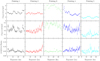 |
Fig. 1. Multi-epoch X-ray time series of RBS 1332. The soft X-rays show a significant variability compatible with flux changes observed above 2 keV. The ratios between hard and soft X-rays also exhibit changes on ks timescales, especially in observations 2 and 5, see the Sect. 2 for model details. Black, red, green, blue, magenta, and cyan colours refer to obs. 1, 2, 3, 4, and 5, respectively. This colour code is adopted throughout the whole paper. |
RBS 1332 was also observed by the Hubble Space Telescope using the Cosmic Origins Spectrograph (COS). This spectrograph (Green et al. 2012) enables one to perform high-sensitivity, medium- and low-resolution (1500–18 000) spectroscopy in the 815–3200 Å wavelength interval. In this case, grating G140L centred at 1280 Å was adopted, enabling us to measure the source emission between 1100 and 2280 Å (observer frame). Final spectra were obtained though the automatic HST/COS calibration pipeline CalCOS.
In Fig. 2, we show the OM and COS rates as observed by XMM-Newton and the HST telescope. Differently to the X-ray flux, no significant flux evolution is observed in the optical/UV during the observational campaign.
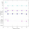 |
Fig. 2. UV light curves obtained using the XMM-Newton optical monitor and HST (FUV). |
3. HST analysis
We started our investigation into the broadband properties of RBS 1332 by characterising its HST spectrum. First, we visually inspected the main UV emission lines in search of relevant absorption features. In doing this, we found that the Lyα, the N V and the C IV transitions were affected by absorption. The position and shape of each trough are similar in all the emission features, with only the ‘red’ Lyα absorption missing. This hints at the fact that such absorption features are produced by material intrinsic to RBS 1332 that is located in the surrounding environment of the AGN central engine; to accurately quantify its properties, we performed a spectral decomposition of every absorbed emission system.
We show the Lyα + N V and C IV spectral regions of each observation in Fig. 3: at a glance, all absorption features appear to be relatively stable in both shape and depth within the spectral noise over the three HST epochs (see Table 1). This implies that the absorber is neither changing in structure (e.g., Krongold et al. 2010; Hall et al. 2011) nor responding to variations in the ionising flux (e.g., Barlow et al. 1992; Trevese et al. 2013) over the course of the HST observations; this allowed us to combine them together by averaging them into a single UV spectrum in the observer-frame interval 1110–2280 Å (corresponding to an interval 990–2030 Å in the rest frame). On this spectrum, we identified intervals that are relatively free of major emission and absorption features, and used them to compute a power-law continuum, Fλ, of the form:

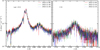 |
Fig. 3. Comparison of the RBS 1332 Lyα + N V and C IV spectral regions in the observer frame over the three HST observation epochs (see legend). Left panel: Lyα + N V spectral region. Right panel: C IV spectral region. |
with α the spectral index. The result fits the RBS 1332 continuous emission well over the entire wavelength interval, with α = −1.37 ± 0.10; therefore, we adopt this fit as a good representation of the actual RBS 1332 continuum in the following analysis of the AGN emission and absorption lines.
During this step, we also identified the presence of two strong emission features bluewards of the Lyα; the most intense one falls at the Lyα rest-frame wavelength of 1215.67 Å, whereas the position of the second one is compatible with that of the O I + Si II system (Vanden Berk et al. 2001). A visual inspection revealed that such features are single Gaussian-like lines rather than being formed by multiple components. These lines are present in all the three HST exposures, and are due to airglow emission that originated as part of the UV sky background1; since they are not relevant for the RBS 1332 spectral analysis, we masked them, and thus excluded them from any calculation. The RBS 1332 average HST spectrum is shown in Fig. 4.
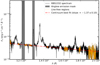 |
Fig. 4. HST spectrum of RBS 1332 (solid black line). The continuum emission (dash-dotted red line) fitted over intervals free of major emission and absorption features (dotted yellow lines) is indicated, along with the masks (grey bands) superimposed on the emission of the UV airglow lines. |
We adopted the power-law shape found in Sect. 3 as our fiducial continuum over the entire spectral interval; on top of this component, we fitted the emission lines using multiple Gaussians:
-
a narrow and a broad component for both the Lyα and the C IV;
-
a single broad component for the N V.
For all components, we left all the parameters free to vary; the goodness of each performed fit was evaluated by computing the χ2 value and the associated degrees of freedom number, νd.o.f.. The results of such fits are shown in Fig. 5. The obtained parameters of the line components are reported in Table 2.
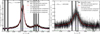 |
Fig. 5. Left panel: Fit to the Lyα + N V emission system of RBS 1332 (see insert). Right panel: Fit to the C IV emission (see insert). In both panels, the main absorption features identified through visual inspections (grey bands) are masked. |
It is immediate to note from Table 2 and Fig. 5 that we did not find evidence of narrow emission components (σ < 600 km s−1) in any of the analyzed transitions. This feature is often found in objects that lie at the bright end of the AGN luminosity function (see e.g. Saturni et al. 2018, and refs. therein); in such cases, forbidden transitions – such as the [O III] λ4959, 5007 doublet – tend to be weak, and an anti-correlation between their intensities and blended Fe II emission (Boroson & Green 1992) is also expected. To investigate the possible weakness of the [O III] λ4959, 5007, we retrieved the RBS 1332 optical spectrum from the SDSS Data Release 16 (DR16; Blanton et al. 2017) portal2, and inspected the Hβ + [O III] spectral region: the [O III] is clearly detected, with both a line width typical of narrow-line regions (NLRs; σ ∼ 250 km s−1) and evidence for a blueshifted broader component, which is also indicative of the presence of an outflow similar to those discovered in other nearby AGNs such as IRAS 20210+1121 (Saturni et al. 2021). Due to these findings, we conclude that the lack of narrow components in the high-ionisation emission lines of RBS 1332 must be ascribed to other physical phenomena; for example, a lowly ionised or stratified NLR (e.g., Wang & Xu 2015).
Best-fit parameters of the RBS 1332 Lyα, N V and C IV emission lines, along with the associated 1σ uncertainties.
3.1. AGN physical parameters of RBS 1332
From the decomposition of the RBS 1332 UV spectrum, we derived all of the physical quantities that describe the AGN central engine. All the results of this paragraph are summarised in Table 3, along with the corresponding 1σ statistical uncertainties. We first computed the monochromatic luminosities at 1350 Å λLλ(1350 Å) and at 1450 Å λLλ(1450 Å) by integrating the RBS 1332 spectrum in 100-Å wide intervals centred around the rest-frame wavelength of interest; then, we used the C IV relation by Vestergaard & Peterson (2006) to derive the SMBH mass, MBH, from λLλ(1350 Å) and the FWHM of the narrower component of the C IV emission line:
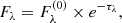
![$$ \begin{aligned} \log {\left( \frac{M_{\rm BH}}{\mathrm{M}_\odot } \right)} = 6.66 + 2 \log {\left( \frac{\mathrm{FWHM}_{\rm CIV}}{1000\,\mathrm{km}\,\mathrm{s}^{-1}} \right)} + 0.53 \log {\left[ \frac{\lambda L_\lambda (1350\,\mathrm{\AA })}{10^{44}\,\mathrm{erg}\,\mathrm{s}^{-1}} \right]} .\end{aligned} $$](/articles/aa/full_html/2025/03/aa52266-24/aa52266-24-eq2.gif)
AGN parameters derived from the analysis of the RBS 1332 C IV spectral region.
In doing so, we note that our estimate of MBH is fully compatible within the uncertainties with the SDSS DR16Q measurement of 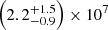 M⊙ (Wu & Shen 2022, see our Table 3); therefore, we decided to adopt it as our fiducial value without applying the correction by Denney (2012) for C IV outflow-induced biases3. From the MBH derived in this way, we estimated the Eddington luminosity, LEdd, of RBS 1332. Subsequently, we adopted the relation by Runnoe et al. (2012a,b) to compute the AGN bolometric luminosity, Lbol, from λLλ(1450 Å):
![$$ \begin{aligned} L_{\rm bol} = 0.75 \times 10^{4.745} \left[ \lambda L_\lambda (1450\,\mathrm{\AA }) \right]^{0.910},\end{aligned} $$](/articles/aa/full_html/2025/03/aa52266-24/aa52266-24-eq4.gif)
and thus the Eddington ratio, εEdd = Lbol/LEdd.
Finally, we assumed the standard accretion disc model by Shakura & Sunyaev (1973) to estimate the maximum black-body temperature, Tmax, of the disc, assuming it reaches the innermost stable circular orbit:
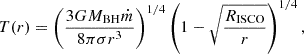
where ṁ is the AGN accretion rate and RISCO = 6GMBH/c2 is the radius of the innermost stable orbit around the (non-rotating) central SMBH. To find Tmax, we estimated ṁ = Lbol/ηc2, adopting a radiative efficiency of η = 0.057 for a non-rotating SMBH (Novikov & Thorne 1973). We took the maximum value assumed by Eq. (4) along the disc radius for our choice of free parameters.
3.2. Parameters of the absorption features associated with the Lyα, N V and C IV transitions
As a next step, we investigated the absorption features associated with the main UV transitions that are present in the RBS 1332 spectrum. To this aim, we first divided the spectrum by the pseudo-continuum obtained by summing all of the emission components derived in the previous steps; then, under the assumption that the AGN emission, Fλ(0), is exponentially absorbed owing to the transport equation (e.g., Rybicki & Lightman 1979),
we empirically modelled the absorption optical depth, τλ, as a sum of Gaussian profiles:
![$$ \begin{aligned} \tau _\lambda = \sum _i A_i \exp {\left[ -\frac{(\lambda - \lambda _i)^2}{2\sigma _i^2} \right]}.\end{aligned} $$](/articles/aa/full_html/2025/03/aa52266-24/aa52266-24-eq7.gif)
The inspection of the Lyα, N V and C IV spectral regions revealed that the Lyα absorption troughs are both formed by two narrower components; also, the intermediate-velocity N V absorption is double, whereas the C IV troughs exhibit simpler single shapes. Therefore, we adopted four Gaussian profiles for both the Lyα and N V absorption, and only three for the C IV one, for a total of 11 components.
We fitted this model to the normalised RBS 1332 spectrum, leaving all the absorption parameters free to vary. The best fits obtained in this way are shown in Fig. 6 for each spectral region, along with the corresponding χ2 and νd.o.f. values. From the fit results, we computed the absorption equivalent widths, EWi, velocity shifts, Δvi, and widths, FWHMi, of each component, along with the corresponding 1σ uncertainties. We report these values in Table 4, numbering each absorption and grouping troughs associated with each transition according to their velocity shift (from blue to red). This leads us to establish the following relations:
-
the most detached ‘blue’ troughs (System 1) all have velocity shifts in the range from −1200 km s−1 to −800 km s−1, with FWHMs in the range of 300 ÷ 600 km s−1;
-
the ‘bluer’ intermediate troughs (System 2) have velocity shifts of −500 ÷ −600 km s−1, with comparable FWHMs of 550 ÷ 650 km s−1 and also similar EWs (around ∼40 km s−1 for both the Lyα and the N V). Interestingly, the C IV transition does not show this absorption component;
-
the ‘redder’ intermediate troughs (System 3) exhibit similar velocity shifts of −150 ÷ −250 km s−1, but more variegated FWHMs that range from ∼250 km s−1 up to ∼1600 km s−1;
-
the ‘red’ troughs (System 4) also have mixed properties in terms of both velocity shifts (from ∼0 to ∼600 km s−1) and spread (FWHMs from ∼400 km s−1 to ∼1200 km s−1), being linked mostly by the fact that they have positive velocity shifts with respect to the transition wavelength and by very similar EWs (all ∼100 km s−1).
Overall, the parameters reported in Table 4 highlight how the analyzed absorption features exhibit intermediate velocity properties between broad (BALs; e.g., Lynds 1967; Weymann et al. 1991) and narrow absorption lines (NALs; e.g., Reynolds 1997; Elvis 2000), in line with those of the so-called mini-BALs (see e.g. Perna et al. 2025, and refs. therein). This interpretation is further supported by the lack of consistent variability over a maximum time interval of Δt ∼ 13 days between the UV observations, corresponding to ∼11.6 days in the rest frame; based on this evidence, under the assumption of a photoionisation-driven absorption variability (Barlow et al. 1992; Trevese et al. 2013), we have been able to put an upper limit on the absorber’s electron density, ne, as:

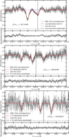 |
Fig. 6. Fits to the absorption systems (dash-dotted red lines) associated with the RBS 1332 major emission features, along with the corresponding standardised residuals. Upper panels: Fit to the Lyα absorption features. Middle panels: Fit to the N V absorption features. Lower panels: Fit to the C IV absorption features. In all panels, the zero-flux level (dotted lines) is indicated, along with the rest-frame position of the relative emission feature (dashed lines). |
Upper section: Parameters of the RBS 1332 absorptions associated with the Lyα, N V and C IV transitions, along with the associated 1σ uncertainties. In all columns, values are expressed in km s−1. Lower section: Minimum column density of the absorbing ions. In all columns, values are expressed in units of 1013 cm−2.
Assuming e.g. αrec = 2.8 × 10⁻¹² cm3 s−1 for the C IV troughs (Arnaud & Rothenflug 1985) and Δtrf > 11.6 days, we got ne < 3.6 × 105 cm−3, which is consistent with the values typically expected for NAL systems (e.g., Elvis 2000; Saturni et al. 2016).
To further quantify the RBS 1332 absorption properties, we estimated the column densities, Nion, associated with each trough (e.g., Savage & Sembach 1991). Under the assumption of an optically thin line lying on the linear part of the curve of growth associated with an absorber with a full covering fraction, the minimum Nion is related to its EW as (e.g., Mehdipour et al. 2023):

where f is the oscillator strength and λ the laboratory wavelength of the transition. We retrieved the values of these quantities from the Atomic Spectra Database v5.124 (Kramida et al. 2024) provided by the National Institute of Standards and Technology (NIST). Based on the EW values that we found for the Lyα, N V and C IV absorptions, we thus computed the corresponding minimum Nion, which is also reported in Table 4. All Nion derived in this way lie in the range of 2 − 12 × 1013 cm−2, in line with typical column densities found for objects with comparable absorption properties (e.g., Wildy et al. 2016; Mehdipour et al. 2023).
The similarities in the physical properties of these absorption systems hint at their common origin, potentially due to the existence of a clumpy (e.g., Dannen et al. 2020; Ward et al. 2024) ionised outflow that is launched outward of the central engine by radiation pressure (e.g., Murray & Chiang 1995; Proga et al. 2000; Risaliti & Elvis 2010), and that then slows down and starts falling back into the AGN. Alternatively, a scenario in which outflow velocities arise from the scattering-off material in a spiralling inflow (Gaskell & Goosmann 2016) may also work. Further multi-wavelength observations and detailed studies that are able to (i) derive the properties of the RBS 1332 UV absorption from prime principles (e.g., by computing numerical models with the CLOUDY software; Ferland et al. 1998), and (ii) relate them to other observable quantities such as the [O III] λ5007 broadening to infer the orientation of the central engine with respect to the line of sight (e.g., Risaliti et al. 2011), are needed to fully understand the physical processes at work behind such features.
4. X-ray spectral analysis
In this section, we report on the broadband spectral fitting that was performed using XSPEC (Arnaud 1996). During the fitting procedure, the hydrogen column density due to the Milky Way, NH = 7.82 × 1019 cm−2 (HI4PI Collaboration 2016), was always included and kept frozen at the quoted value. When COS and OM data are analysed, extinction is taken into account and we assumed E(B–V) = 0.0067 (Schlafly & Finkbeiner 2011). We assumed the standard cosmology ΛCDM framework with H0 = 70 km s−1 Mpc−1, Ωm = 0.27, and Ωλ = 0.73.
The X-ray emission of RBS 1332 is dominated by a prominent and variable soft X-ray emission that exceeds the steep (Γ > 2) primary continuum. In Fig. 7, we show the residuals to a power-law component fitting only the 3–10 keV energy range. Interestingly, no features ascribable to a Fe Kα emission line are observed (see inset in Fig. 7). Previous analyses aiming to characterise the physical origin of the soft X-ray excess in AGNs have focused on X-ray data only. However, such an approach has been found to be inconclusive as the main competing scenarios give a similar best-fit quality for the X-ray emission (e.g. García et al. 2019). However, they provide different estimates for the UV emission; thus, in the following, we directly work on our broadband UV to X-ray dataset.
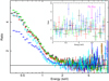 |
Fig. 7. Ratios of the XMM-Newton data to a power law fitting the 3–10 keV energy range. A variable and remarkable soft excess is clearly present below 3 keV, while no hints of a Fe Kα emission line are observed. |
4.1. Testing relativistic reflection
As has been stated, our dataset extends down to the UV domain; hence, in the modelling, we need to include any possible contribution from the broad-line region (BLR) that is responsible for the excess of photons observed around 3000 Å, the so-called small blue bump (SBB). We considered this spectral component using an additive table within XSPEC that was already presented in Mehdipour et al. (2015). During the fitting procedure, the normalisation of the SBB was free to vary (but tied among the observations). From the fit, we obtained a flux of F0.001 − 0.01 keV = (8.7 ± 0.3)×10−13 erg s−1 cm−2 for this component. This flux is quantitatively compatible within the errors with the one obtaining by integrating the differential continuum derived in Sect. 3 from the HST data.
Despite the lack of a significant Fe Kα feature, we tested relativistic reflection as the origin of the X-ray soft excess in RBS 1332. At this stage, a reflection component cannot be ruled out as the lack of evidence of a Fe K feature can be explained by the presence of an extremely broad iron line that is hard to detect in limited S/N data. Moreover, very weak Fe K emission line is expected when specific disc properties are met (e.g. high ionisation García et al. 2014), or in the presence of relativistic effects near a maximally spinning BH (Crummy et al. 2006), or simply by the very soft shape of the X-rays.
Thus, we started modelling the hard X-ray continuum with THCOMP, a convolution model meant to replace NHTCOMP (Magdziarz & Zdziarski 1995; Zdziarski et al. 1996; Życki et al. 1999). This model describes a Comptonisation spectrum by thermal electrons emitted by a spherical source and accounts for a sinusoidal-like spatial distribution of the seed photons, like in COMPST (Sunyaev & Titarchuk 1980). THCOMP describes both upscattering and downscattering radiation and as a convolution model it can be used to Comptonise any seed photon distribution. In our case, we assumed that the seed radiation emerges from a DISKBB component used to provide a standard spectrum from a multi-temperature accretion disc. Within THCOMP, it is possible to compute the photon index, Γ, the temperature of the seed photons, and a covering fraction, 0 ≤ covfrac ≤ 1. When set to 1, all of the seed photons are Comptonised by the plasma, while below 1, only a fraction of the seed photons are energised. In our computations, we left covfrac free to vary. We then linked to this continuum emission a relativistic reflection component using RELXILLCP (e.g. García et al. 2014) and assumed the photon index of the two components to be the same. RELXILLCP combines the XILLVER reflection code and the RELLINE ray tracing code (e.g. Dauser et al. 2016) and returns a spectrum due to irradiation of the accretion disc by an incident Comptonised continuum. Written in XSPEC notation, this model reads as:

For each exposure of the monitoring, we calculated the source photon index, Γ (linking this parameter between THCOMP and RELXILLCP), the temperature of the accretion disc (Tbb (eV)), and its normalisation. For RELXILLCP, the ionisation parameter, log ξ (1/erg cm−2 s−1), and its normalisation were fitted for each exposure. On the other hand, the iron abundance, AFe, the disc inclination, incl°, the BH spin (a), and the coronal emissivity (index1) were, instead, fitted, tying their values among the observations. The covering fraction of the Comptonising plasma was also fitted, linking its value among the pointings.
This approach led us to a fit statistic of χ2 = 882 for 691 d.o.f.; we show the corresponding fit and its accompanying quantities in Fig. 8 and Table 5, respectively.
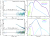 |
Fig. 8. Top panels: Broadband fit to the OM, COS, and EPIC-pn data assuming the soft X-ray excess to be dominated by relativistic reflection (top left ). In the top right panel, we show the different contributions to the overall emission spectrum of RBS 1332 for each of the model components inferred from Obs. 1. Bottom panels: Broadband fit of the same dataset, assuming the soft X-ray excess to be dominated by a warm Comptonisation (left panel). Right panel: Different contribution to the overall emission spectrum of RBS 1332 derived from the first observation of our observational campaign. |
Best-fit parameters derived for the relativistic reflection scenario. Errors are given at a 90% confidence level for the single parameter of interest.
In accordance with this model, the broadband emission of RBS 1332 can be ascribed to a black-body-like emission that dominates the FUV and UV wavelengths. No significant changes in its temperature are observed. In this depicted scenario, only a marginal fraction of the photons emitted by the disc are Comptonised by the hot corona (covfrac ∼ 7%) and the X-rays can mainly be ascribed to extreme relativistic reflection. A very steep emissivity is found (index1 > 8.85), implying that the Comptonising plasma is very close to the maximally rotating SMBH (a > 0.997).
4.2. Testing warm Comptonisation
As an alternative to blurred ionised reflection, we tested the two-coronae model (e.g. Petrucci et al. 2018; Kubota & Done 2018). Within this framework, the broadband emission spectrum of AGN is accounted for by distinct emitting zones: a standard accretion disc; a warm Comptonising plasma; and the inner hot corona. In particular, the disc can be either non-dissipative and in this case be fully covered by the warm corona, or instead contribute to the overall flux of the source. In this second scenario, the warm corona is assumed to be patchy and part of the energy has dissipated in the disc, leaked through the warm coronal region. The warm corona is defined as an optically thick and geometrically thin medium in which Comptonisation is the dominant cooling mechanism (Petrucci et al. 2018, 2020), while the hot corona is the one standard depicted in the two-phase model. We thus modified our previously adopted test model as follows:

Thus, we modelled the broadband emission spectrum of RBS 1332, assuming an outer disc for which we computed its temperature (Tbb), linking its value among the observations. The normalisation, Normdisc, was instead derived in each observation. Then, we assumed the soft X-rays to be emerging from a closer region in which a fraction of disc photons are Comptonised (thcompw × diskbb). For this second component, we fitted the photon index, the temperature and normalisation of the disc photons, the covering fraction of the warm corona, and its normalisation. Finally, for the hot corona we assumed that the seed photons cooling it are only those from the warm component (T ). We fixed the hot corona temperature to a constant value of kT = 50 keV, in agreement with average estimates (e.g. Middei et al. 2019a; Kamraj et al. 2022). Thus, we only fitted the photon index, ΓH, and the model normalisation. These simple steps led us to a best fit of χ2/d.o.f. = 739/680, which is shown in the bottom panels of Fig. 8.
Best-fit parameters corresponding to the two-coronae fitting model. The fluxes and luminosity are the observed ones.
This best fit to the data agrees with the optical-to-X-ray emission of RBS 1332 emerging from three distinct components. First, there is a hot corona with a soft spectral index (Γhard ∼ 2.2). Then, there is a warm corona region characterised by an average spectral index steeper than the primary continuum (Γsoft ∼ 2.65) and an average temperature of kTwarm ∼ 0.2 keV. These values can be translated into a Thompson opacity5 of τwarm ∼ 30. These inferred parameters for the warm corona are in full agreement with the bulk of measurements reported by Petrucci et al. (2018). Finally, we added a standard disc responsible for the optical emission, part of which is Comptonised by the hot corona. In Table 7, we show the relative flux of the various components used to model the UV-to-X-ray spectra of RBS 1332, and in Fig. 9 we show the corresponding emission components. The best-fit temperature of the accretion disc, Tin ∼ 1.2 eV, is a factor of ∼10 less than the Tmax reported in Table 3; however, we remark that Tmax is just the upper limit of the range of BB temperatures achievable by an optically thick and geometrically thin accretion disc (Shakura & Sunyaev 1973). Furthermore, the Tmax derived from the UV spectral analysis is only a factor of ∼2 lower than the average Tbb ∼ 30 eV – corresponding to ∼3.5 × 10⁵ K – found for the BB component of the warm corona. Based on this evidence, we conclude that all the gas temperatures obtained from the UV and X-ray analyses are in line with the typical values expected for accretion-powered AGN activity.
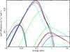 |
Fig. 9. Three components shaping the broadband emission of RBS 1332 are shown for each observation of the campaign. |
Fluxes for the different emission components adopted to model the broadband emission of RBS 1332 assuming the two-coronae model.
In the context of the two-coronae model, we find that the disc component is fairly constant during the campaign, while both the hard power law and the warm corona changes in flux by a compatible amount. As a final test, we fitted the broadband data of RBS 1332 using the model AGNSED, (Done et al. 2012; Kubota & Done 2018). Within this model, the three distinct emitting zones (outer disc, warm corona, and hot corona) are energetically coupled and assumed to be radially stratified. The first one emits as a standard disc black body (BB) from Rout to Rwarm, as warm Comptonisation from Rwarm to Rhot (see Petrucci et al. 2018, 2020, for details on this region), and, below Rhot down to RISCO, as the typical geometrically thick, optically thin electron distributions expected to provide the AGN hard X-ray continuum (Haardt & Maraschi 1993). Radii are in units of gravitational radii, Rg. In the fitting procedure, we calculated the hard and the warm corona photon indices (Γhard and Γsoft), and the warm coronal temperature, kTe (keV), while the hard coronal temperature was kept to a fixed value of 50 keV. A co-moving distance of 539 Mpc was derived from the redshift and fixed in the model. We assumed a SMBH mass of log MBH = 7.2 ± 0.2, based on our computations from the UV spectrum in Sect. 3. We set the scale height for the hot Comptonisation component, HTmax, to 10 gravitational radii, Rg, this mimicking a spherical Comptonising plasma of a similar radius. Finally, we assumed a disc inclination of 30° and a spin of 0.5. This led us to a best fit of χ2 = 785 for 691 d.o.f., which is fully compatible with the one previously obtained. The spectral indices of the hot and warm Comptonisation regions are in good agreement with those in Table 6 found in the previous warm Comptonisation fit. This fit provides estimates of the size of the different regions of emission. The hot corona appears to be quite compact (∼10 Rg), while the warm Comptonisation area extends up to ∼200 Rg (see Table 8). We note, however, variations in this radius, Rwarm, of a factor of 4 in the five observations, while the hot coronal region remains more constant. The derived Eddington ratio is in the range of ∼25 − 55% Eddington.
Radial extension in gravitational radii derived from AGNSED.
4.3. Warm corona or relativistic reflection
We complemented the analyses presented in previous Sects 4.1 and 4.2, testing REXCOR6 (Xiang et al. 2022; Ballantyne et al. 2024), a spectral model that self-consistently calculates the effects of both ionised relativistic reflection (incorporating the light bending and line blurring) and the emission from a warm corona. Within REXCOR, the accretion power released in the inner regions of the accretion disc (< 400 rg) is distributed among a hot corona (for wich a lamppost geometry is assumed), a warm corona, and the accretion disc itself. The model REXCOR accounts for a plethora of shapes for the soft X-ray excess that depends on the amount of energy dissipated either by the lamppost or the warm corona.
This model can be used in XSPEC as additive tables that were computed for fixed values of the BH spin (0.9, 0.99), lamppost height (5 Rg, 20 Rg), and Eddington ratio (1%, 10%). Up to five parameters can be fitted in these tables: the fraction of the accretion flux dissipated in the lamppost (fx), the photon index of the power-law continuum (Γ), the fraction of the accretion flux dissipated in the warm corona (hf), the warm corona opacity, τ, and the model normalisation. Then, we tested on our dataset the following XSPEC model:
We fitted the temperature of the DISKBB component, linking its value among the observations while its normalisation was computed for each dataset. The fraction of the energy dissipated in the lamppost, the warm corona, as well as the opacity of this second component and the model normalisation, were free to vary and fitted for each epoch. We tied the photon index of REXCOR to the one of NTHCOMP and computed it. Concerning NTHCOMP, we assumed its T(bb) temperature to be the same as the disc, while the temperature of the hot electron was fixed to 50 keV. We started fitting the REXCOR table considering the full XMM-Newton band but, due to the limited gamma range (1.5 < Γ < 2.2) allowed in the model, it struggles to account for the very first soft bins of the spectra. Consequently, we excluded data below 0.5 keV and re-fitted the spectra, obtaining a better fit statistic of χ2 = 760/663, which is statistically compatible with the one obtained with the two-coronae model. We found that our choice of ignoring data below 0.5 keV does not modify the best-fit values for the fraction of energies dissipated in the lamppost or the warm corona. For the sake of simplicity, in Table 9 we only report the quantities derived for the REXCOR table, as the other parameters are consistent within the errors with the previously obtained values.
Results of the REXCOR model on the RBS 1332 dataset.
The use of the REXCOR model supports the interpretation that the soft X-ray excess is mainly due to inverse-Compton scattering. In fact, for each exposure, the fraction of accretion power dissipated within the warm corona is several times greater than the cooling due to the lamppost.
5. Discussion and conclusions
We have reported on the first HST/XMM-Newton monitoring campaign of the US-NLSy1 galaxy RBS 1332. In the following, we summarise and discuss our findings.
Variability properties: In the observations, the source shows significant flux variability of about 30% on hourly timescales and up to a factor of 4 in about 10 days (see Fig. 1). The amount of change is compatible between the soft (0.5–2 keV) and the hard (2–10 keV) X-rays bands, as no significant spectral changes are witnessed during the exposures. Moreover, neither the UV nor the FUV data seem to vary during the observational campaign (see Fig. 2).
Given the compatible flux observed in the soft X-ray and ultraviolet bands (e.g. Table 7), one could expect the variable soft X-rays to illuminate the outer disc and induce variability in the optical/UVs. In particular, the X-ray reprocessing would cause optical/UV reverberation lags, as has been observed in long and richly sampled light curves of AGNs (e.g. Mason et al. 2002; Arévalo et al. 2005; Alston et al. 2013; Lohfink et al. 2014; Edelson et al. 2015, 2019; Buisson et al. 2017; Cackett et al. 2023). The lack of variability we observe in the optical/UV bands can be explained by the short timescales investigated here, at which X-rays variations are likely smeared in the outer disc, with this weakening any signal associated with reverberation (e.g. Smith & Vaughan 2007; Robertson et al. 2015; Kammoun et al. 2021). Any possible reverberated signal would, in fact, be diluted by the intrinsic UV emission (see Jin et al. (2017b) for a thorough discussion on this subject).
5.1. Black hole mass estimates
The significant variability of the X-ray light curve can be used to estimate the SMBH mass. Both long and short term X-ray variability was found to be anti-correlated with the AGN’s luminosity and black hole mass (Barr & Mushotzky 1986; Green et al. 1993; Lawrence & Papadakis 1993; Markowitz et al. 2003; Papadakis 2004; McHardy et al. 2006; Vagnetti et al. 2016; Paolillo et al. 2023). Thus, we computed the light curves of RBS 1332 for all the available observations, including the archival ones (obs. IDs 0741390201 and 0741390401), and extracted all the 2–10 keV light curves with a time bin of 500 s. Then, we calculated in each 20 ks-long segment the normalised excess variance (Vaughan et al. 2003), which we found to be  . Using the relations by Ponti et al. (2012), Tortosa et al. but see also 2023, this quantity yields to a BH mass of MBH = (7.4 ± 1.0)×106 M⊙. This estimate, which is compatible with previous values using the L5100 Å and FWHMHβ (see discussion in Xu et al. 2021), is about a factor of 2 smaller than the one inferred from the FUV analysis in Sect. 3.1 or with the single epoch estimate by Wu & Shen (2022). Considering an average value for the 2–10 keV luminosity and adopting the bolometric correction by Duras et al. (2020), we obtain a bolometric luminosity of LBol = 8.4 × 1044 erg s−1. This value, coupled with the BH mass derived from the normalised excess variance, leads to an Eddington ratio of 90%, which is about a factor of 2 larger than the one derived from the analysis of the FUV spectrum.
The discrepancy between the two values of the Eddington ratio can easily be reconciled by the fact that objects with high accretion rates (super-Eddington accreting massive black holes, SEAMBHs) – from significant Eddington fractions to the super-Eddington regime – have been found to possess smaller BLR sizes with respect to normal quasars (Du et al. 2015), which is probably related to altered disc and torus geometries. This in turn implies a higher BLR velocity dispersion, and thus a systematic overestimation of the MBH value derived from single-epoch relations in the case of SEAMBHs. Hence, the difference in our MBH values could easily be ascribed to accretion processes close to the Eddington limit powering the RBS 1332 central engine and shaping its internal structure accordingly (see also Jin et al. 2017b). We note that our results, with the exception of AGNSED, do not depend on the BH mass and that, irrespective of the value of the BH mass we may adopt, RBS 1332 is compatible with being efficiently accreting matter.
5.2. Properties of the UV absorption features
The main UV high-ionisation transitions – Lyα, N Vλ1241 and C IVλ1549 – all show absorption features extended over a wide range of velocities, spanning ∼3200 km s−1 from ∼–1500 km s−1 to ∼1700 km s−1. These features do not vary over a time span of ∼11.6 rest-frame days, implying electron densities of ne < 3.6 × 105 cm−3 under the assumption of a photoionisation-driven absorption variability (Barlow et al. 1992; Trevese et al. 2013). Despite their moderate EWs (from ∼40 km s−1 to ∼130 km s−1, corresponding to minimum column densities of 2–12 × 1013 cm−2), the presence of such troughs, together with the evidence of blueshifted emission-line wings associated with forbidden transitions (see e.g. Saturni et al. 2021), points to the existence of a mildy ionised outflow powered by the RBS 1332 central engine, which can be further studied with dedicated investigations of its physical properties and geometry.
Such winds are ubiquitous in AGNs at several redshifts (e.g., Kakkad et al. 2016, 2018) and luminosities (e.g., Vietri et al. 2018), often extending to the whole host galaxy (e.g., Perna et al. 2015, 2017), and thus they play an important role in regulating AGN activity and star formation by altering the amount of available gas for both these processes (e.g., Cattaneo et al. 2009; Fabian 2012). Investigating with future dedicated studies the nature of the outflow at work in the RBS 1332 environment will therefore be crucial to understanding its impact on the host galaxy environment and evolution (e.g., Cicone et al. 2018).
5.3. Spectral modelling and the global picture
We tested four different models to account for the multi-epoch UV-to-X-ray data obtained in the context of our monitoring campaign: blurred relativistic reflection, warm Comptonisation (also including AGNSED), and a model that combines both (relativistic reflection and warm-Comptonisation), REXCOR. In the relativistic reflection scenario, the X-ray emission is in fact dominated by reflection, and the observed variability is mostly due to changes in the reflected flux. This could in turn be related to variations in the geometry of the disc-corona; for example, if the corona is a lamppost source, a variation in the coronal height above the disc would imply a variation in the solid angle subtended by the disc.
However, we find that the broadband emission spectrum and the soft X-ray excess are statistically best modelled in the framework of the two-coronae model. A similar conclusion was drawn by Xu et al. (2021) using Swift and XMM-Newton archival exposures.
We have found the overall emission spectrum of RBS 1332 emerges from three distinct components: i) a fairly constant outer disc (≤200 Rg) with Tdisc ∼ 1 eV; ii) a patchy warm corona Compton up-scattering about ∼20% of the underlying seed photons and extending from about 10 Rg to ∼200 Rg); and iii) a very compact (≤10 Rg) hot corona with a soft spectrum. The physical and geometrical parameters of the hot corona are moderately variable during the campaign, as is indicated by the fits with AGNSED and REXCOR. Also, the radial extension of the warm corona shows a significant variability and is positively correlated with the accretion rate, while there is no clear trend with its temperature or optical depth. The same results were obtained by Palit et al. (2024) for a sample of Seyfert galaxies. Despite the extreme soft X-ray excess observed in this source, its photon index, the temperature, and the opacity are fairly standard when compared with results from other monitoring campaigns (Ursini et al. 2018, 2020; Middei et al. 2018, 2019b, 2020; Porquet et al. 2018), archival studies (Petrucci et al. 2018, 2020; Xiang et al. 2022; Ballantyne et al. 2024; Palit et al. 2024), and distant quasars (Marinucci et al. 2022; Vaia et al. 2024).
The extension of the hot corona appears to be compact (Rhot ∼ 10 Rg) and characterised by the ultra-soft observed hard power law (Γ ∼ 2.2). This can possibly be explained by the interplay between a small heating power sustaining the hot corona and the efficient cooling due to the large fraction of seed photons from the warm corona. An other possibility is provided by the presence of a puffed-up disc layer between the warm coronal region and the outer disc (Jin et al. 2017b). This bloated layer of matter would be illuminated by the hard continuum, part of which could either pierce through it, reaching the outer disc or being reprocessed and eventually producing a weak reflection signal.
Finally, although limited by the moderate parameter range in the available REXCOR tables, we found that the soft X-ray excess in RBS,1332 is primarily attributable to warm Comptonisation, with reprocessing of the primary continuum playing only a marginal role. This analysis, along with the findings by Jin et al. (2017a), further supports the two-coronae model as a viable explanation for the multi-wavelength emission spectrum of extreme AGNs like the US-NLSy galaxies.
Estimating MBH with the Denney (2012) relation from the C IV FWHM computed over the entire line profile would yield (1.0 ± 0.4)×107 M⊙, i.e. a factor of ≳2 lower than the SDSS value.
REXCOR is freely available for spectral fitting using XSPEC at the webpage https://github.com/HEASARC/xspec_localmodels/tree/master/reXcor
Acknowledgments
We thank the anonymous referee for their thorough reading of the manuscript. RM acknowledges Ioanna Psaradaki for insightful discussions on the UV spectra and acknowledges financial support from the ASI–INAF agreement n. 2022-14-HH.0. SB is an overseas researcher under the Postdoctoral Fellowship of Japan Society for the Promotion of Science (JSPS), supported by JSPS KAKENHI Grant Number JP23F23773. This work relies on archival data, software or online services provided by the Space Science Data Center – ASI, and it is based on observations obtained with XMM-Newton, an ESA science mission with instruments and contributions directly funded by ESA Member States and NASA.POP and MC acknowledges financial support from the High Energy french National Programme (PNHE) of the National Center of Scientific research (CNRS) and from the french spatial agency (CNES). BDM acknowledges support via Ramón y Cajal Fellowship (RYC2018-025950-I), the Spanish MINECO grants PID2022-136828NB-C44 and PID2020-117252GB-I00, and the AGAUR/Generalitat de Catalunya grant SGR-386/2021.
References
- Alston, W. N., Vaughan, S., & Uttley, P. 2013, MNRAS, 435, 1511 [NASA ADS] [CrossRef] [Google Scholar]
- Arévalo, P., Papadakis, I., Kuhlbrodt, B., & Brinkmann, W. 2005, A&A, 430, 435 [NASA ADS] [CrossRef] [EDP Sciences] [Google Scholar]
- Arnaud, K. A. 1996, in Astronomical Data Analysis Software and Systems V, eds. G. H. Jacoby, & J. Barnes, ASP Conf. Ser., 101, 17 [NASA ADS] [Google Scholar]
- Arnaud, M., & Rothenflug, R. 1985, A&AS, 60, 425 [NASA ADS] [Google Scholar]
- Bade, N., Fink, H. H., Engels, D., et al. 1995, A&AS, 110, 469 [NASA ADS] [Google Scholar]
- Ballantyne, D. R., Sudhakar, V., Fairfax, D., et al. 2024, MNRAS, 530, 1603 [NASA ADS] [CrossRef] [Google Scholar]
- Barlow, T. A., Junkkarinen, V. T., Burbidge, E. M., et al. 1992, ApJ, 397, 81 [NASA ADS] [CrossRef] [Google Scholar]
- Barr, P., & Mushotzky, R. F. 1986, Nature, 320, 421 [NASA ADS] [CrossRef] [Google Scholar]
- Bianchi, S., Guainazzi, M., Matt, G., Fonseca Bonilla, N., & Ponti, G. 2009, A&A, 495, 421 [NASA ADS] [CrossRef] [EDP Sciences] [Google Scholar]
- Blanton, M. R., Bershady, M. A., Abolfathi, B., et al. 2017, AJ, 154, 28 [Google Scholar]
- Boroson, T. A., & Green, R. F. 1992, ApJS, 80, 109 [Google Scholar]
- Buisson, D. J. K., Lohfink, A. M., Alston, W. N., & Fabian, A. C. 2017, MNRAS, 464, 3194 [Google Scholar]
- Cackett, E. M., Gelbord, J., Barth, A. J., et al. 2023, ApJ, 958, 195 [NASA ADS] [CrossRef] [Google Scholar]
- Cattaneo, A., Faber, S. M., Binney, J., et al. 2009, Nature, 460, 213 [NASA ADS] [CrossRef] [Google Scholar]
- Cicone, C., Brusa, M., Ramos Almeida, C., et al. 2018, Nat. Astron., 2, 176 [Google Scholar]
- Crummy, J., Fabian, A. C., Gallo, L., & Ross, R. R. 2006, MNRAS, 365, 1067 [Google Scholar]
- Dannen, R. C., Proga, D., Waters, T., & Dyda, S. 2020, ApJ, 893, L34 [Google Scholar]
- Dauser, T., García, J., Walton, D. J., et al. 2016, A&A, 590, A76 [NASA ADS] [CrossRef] [EDP Sciences] [Google Scholar]
- Denney, K. D. 2012, ApJ, 759, 44 [NASA ADS] [CrossRef] [Google Scholar]
- Done, C., Davis, S. W., Jin, C., Blaes, O., & Ward, M. 2012, MNRAS, 420, 1848 [Google Scholar]
- Du, P., Hu, C., Lu, K.-X., et al. 2015, ApJ, 806, 22 [NASA ADS] [CrossRef] [Google Scholar]
- Duras, F., Bongiorno, A., Ricci, F., et al. 2020, A&A, 636, A73 [NASA ADS] [CrossRef] [EDP Sciences] [Google Scholar]
- Edelson, R., Gelbord, J. M., Horne, K., et al. 2015, ApJ, 806, 129 [NASA ADS] [CrossRef] [Google Scholar]
- Edelson, R., Gelbord, J., Cackett, E., et al. 2019, ApJ, 870, 123 [NASA ADS] [CrossRef] [Google Scholar]
- Elvis, M. 2000, ApJ, 545, 63 [NASA ADS] [CrossRef] [Google Scholar]
- Fabian, A. C. 2012, ARA&A, 50, 455 [Google Scholar]
- Fabian, A. C., Lohfink, A., Kara, E., et al. 2015, MNRAS, 451, 4375 [Google Scholar]
- Ferland, G. J., Korista, K. T., Verner, D. A., et al. 1998, PASP, 110, 761 [Google Scholar]
- Gallo, L. 2018, Revisiting Narrow-Line Seyfert 1 Galaxies and their Place in the Universe, 34 [Google Scholar]
- García, J., Dauser, T., Lohfink, A., et al. 2014, ApJ, 782, 76 [Google Scholar]
- García, J. A., Kara, E., Walton, D., et al. 2019, ApJ, 871, 88 [CrossRef] [Google Scholar]
- Gaskell, C. M., & Goosmann, R. W. 2016, Ap&SS, 361, 67 [NASA ADS] [CrossRef] [Google Scholar]
- George, I. M., & Fabian, A. C. 1991, MNRAS, 249, 352 [Google Scholar]
- Gliozzi, M., & Williams, J. K. 2020, MNRAS, 491, 532 [Google Scholar]
- Goodrich, R. W. 1989, ApJ, 342, 224 [Google Scholar]
- Green, A. R., McHardy, I. M., & Lehto, H. J. 1993, MNRAS, 265, 664 [NASA ADS] [Google Scholar]
- Green, J. C., Froning, C. S., Osterman, S., et al. 2012, ApJ, 744, 60 [NASA ADS] [CrossRef] [Google Scholar]
- Grupe, D., Wills, B. J., Leighly, K. M., & Meusinger, H. 2004, AJ, 127, 156 [NASA ADS] [CrossRef] [Google Scholar]
- Grupe, D., Komossa, S., Leighly, K. M., & Page, K. L. 2010, ApJS, 187, 64 [NASA ADS] [CrossRef] [Google Scholar]
- Haardt, F., & Maraschi, L. 1991, ApJ, 380, L51 [Google Scholar]
- Haardt, F., & Maraschi, L. 1993, ApJ, 413, 507 [Google Scholar]
- Hall, P. B., Anosov, K., White, R. L., et al. 2011, MNRAS, 411, 2653 [NASA ADS] [CrossRef] [Google Scholar]
- HI4PI Collaboration (Ben Bekhti, N., et al.) 2016, A&A, 594, A116 [NASA ADS] [CrossRef] [EDP Sciences] [Google Scholar]
- Jiang, J., Gallo, L. C., Fabian, A. C., Parker, M. L., & Reynolds, C. S. 2020, MNRAS, 498, 3888 [NASA ADS] [CrossRef] [Google Scholar]
- Jin, C., Done, C., & Ward, M. 2017a, MNRAS, 468, 3663 [NASA ADS] [CrossRef] [Google Scholar]
- Jin, C., Done, C., Ward, M., & Gardner, E. 2017b, MNRAS, 471, 706 [NASA ADS] [CrossRef] [Google Scholar]
- Kakkad, D., Mainieri, V., Padovani, P., et al. 2016, A&A, 592, A148 [NASA ADS] [CrossRef] [EDP Sciences] [Google Scholar]
- Kakkad, D., Groves, B., Dopita, M., et al. 2018, A&A, 618, A6 [NASA ADS] [CrossRef] [EDP Sciences] [Google Scholar]
- Kammoun, E. S., Papadakis, I. E., & Dovčiak, M. 2021, MNRAS, 503, 4163 [CrossRef] [Google Scholar]
- Kamraj, N., Brightman, M., Harrison, F. A., et al. 2022, ApJ, 927, 42 [NASA ADS] [CrossRef] [Google Scholar]
- Kramida, A., Ralchenko, Yu., Reader, J., and NIST ASD Team 2024, NIST Atomic Spectra Database (version 5.12), https://dx.doi.org/10.18434/T4W30F [Google Scholar]
- Krongold, Y., Binette, L., & Hernández-Ibarra, F. 2010, ApJ, 724, L203 [NASA ADS] [CrossRef] [Google Scholar]
- Kubota, A., & Done, C. 2018, MNRAS, 480, 1247 [Google Scholar]
- Lawrence, A., & Papadakis, I. 1993, ApJ, 414, L85 [NASA ADS] [CrossRef] [Google Scholar]
- Lohfink, A. M., Reynolds, C. S., Vasudevan, R., Mushotzky, R. F., & Miller, N. A. 2014, ApJ, 788, 10 [NASA ADS] [CrossRef] [Google Scholar]
- Lynds, C. R. 1967, ApJ, 147, 396 [NASA ADS] [CrossRef] [Google Scholar]
- Magdziarz, P., & Zdziarski, A. A. 1995, MNRAS, 273, 837 [Google Scholar]
- Malizia, A., Molina, M., Bassani, L., et al. 2014, ApJ, 782, L25 [NASA ADS] [CrossRef] [Google Scholar]
- Mallick, L., Alston, W. N., Parker, M. L., et al. 2018, MNRAS, 479, 615 [NASA ADS] [Google Scholar]
- Marinucci, A., Vietri, G., Piconcelli, E., et al. 2022, A&A, 666, A169 [NASA ADS] [CrossRef] [EDP Sciences] [Google Scholar]
- Markowitz, A., Edelson, R., Vaughan, S., et al. 2003, ApJ, 593, 96 [NASA ADS] [CrossRef] [Google Scholar]
- Mason, K. O., Breeveld, A., Much, R., et al. 2001, A&A, 365, L36 [NASA ADS] [CrossRef] [EDP Sciences] [Google Scholar]
- Mason, K. O., McHardy, I. M., Page, M. J., et al. 2002, ApJ, 580, L117 [NASA ADS] [CrossRef] [Google Scholar]
- Matzeu, G. A., Nardini, E., Parker, M. L., et al. 2020, MNRAS, 497, 2352 [CrossRef] [Google Scholar]
- McHardy, I. M., Koerding, E., Knigge, C., Uttley, P., & Fender, R. P. 2006, Nature, 444, 730 [NASA ADS] [CrossRef] [Google Scholar]
- Mehdipour, M., Kaastra, J. S., Kriss, G. A., et al. 2015, A&A, 575, A22 [NASA ADS] [CrossRef] [EDP Sciences] [Google Scholar]
- Mehdipour, M., Kriss, G. A., Kaastra, J. S., Costantini, E., & Mao, J. 2023, ApJ, 952, L5 [NASA ADS] [CrossRef] [Google Scholar]
- Middei, R., Bianchi, S., Cappi, M., et al. 2018, A&A, 615, A163 [NASA ADS] [CrossRef] [EDP Sciences] [Google Scholar]
- Middei, R., Bianchi, S., Marinucci, A., et al. 2019a, A&A, 630, A131 [NASA ADS] [CrossRef] [EDP Sciences] [Google Scholar]
- Middei, R., Bianchi, S., Petrucci, P. O., et al. 2019b, MNRAS, 483, 4695 [NASA ADS] [CrossRef] [Google Scholar]
- Middei, R., Petrucci, P. O., Bianchi, S., et al. 2020, A&A, 640, A99 [NASA ADS] [CrossRef] [EDP Sciences] [Google Scholar]
- Middei, R., Petrucci, P. O., Bianchi, S., et al. 2023, A&A, 672, A101 [NASA ADS] [CrossRef] [EDP Sciences] [Google Scholar]
- Murray, N., & Chiang, J. 1995, ApJ, 454, L105 [NASA ADS] [Google Scholar]
- Nardini, E., Lusso, E., & Bisogni, S. 2019, MNRAS, 482, L134 [Google Scholar]
- Novikov, I. D., & Thorne, K. S. 1973, Black Holes (Les Astres Occlus), 343 [Google Scholar]
- Osterbrock, D. E. 1977, ApJ, 215, 733 [Google Scholar]
- Padovani, P., Alexander, D. M., Assef, R. J., et al. 2017, A&ARv, 25, 2 [Google Scholar]
- Palit, B., Różańska, A., Petrucci, P. O., et al. 2024, A&A, 690, A308 [NASA ADS] [CrossRef] [EDP Sciences] [Google Scholar]
- Paolillo, M., Papadakis, I. E., Brandt, W. N., et al. 2023, A&A, 673, A68 [NASA ADS] [CrossRef] [EDP Sciences] [Google Scholar]
- Papadakis, I. E. 2004, MNRAS, 348, 207 [NASA ADS] [CrossRef] [Google Scholar]
- Perna, M., Brusa, M., Cresci, G., et al. 2015, A&A, 574, A82 [NASA ADS] [CrossRef] [EDP Sciences] [Google Scholar]
- Perna, M., Lanzuisi, G., Brusa, M., Cresci, G., & Mignoli, M. 2017, A&A, 606, A96 [NASA ADS] [CrossRef] [EDP Sciences] [Google Scholar]
- Perna, M., Arribas, S., Ji, X., et al. 2025, A&A, 694, A170 [NASA ADS] [CrossRef] [EDP Sciences] [Google Scholar]
- Perola, G. C., Matt, G., Fiore, F., et al. 2000, A&A, 358, 117 [NASA ADS] [Google Scholar]
- Petrucci, P. O., Paltani, S., Malzac, J., et al. 2013, A&A, 549, A73 [NASA ADS] [CrossRef] [EDP Sciences] [Google Scholar]
- Petrucci, P. O., Ursini, F., De Rosa, A., et al. 2018, A&A, 611, A59 [NASA ADS] [CrossRef] [EDP Sciences] [Google Scholar]
- Petrucci, P. O., Gronkiewicz, D., Rozanska, A., et al. 2020, A&A, 634, A85 [NASA ADS] [CrossRef] [EDP Sciences] [Google Scholar]
- Piconcelli, E., Jimenez-Bailón, E., Guainazzi, M., et al. 2004, MNRAS, 351, 161 [Google Scholar]
- Ponti, G., Papadakis, I., Bianchi, S., et al. 2012, A&A, 542, A83 [NASA ADS] [CrossRef] [EDP Sciences] [Google Scholar]
- Porquet, D., Reeves, J. N., Matt, G., et al. 2018, A&A, 609, A42 [NASA ADS] [CrossRef] [EDP Sciences] [Google Scholar]
- Porquet, D., Reeves, J. N., Grosso, N., Braito, V., & Lobban, A. 2021, A&A, 654, A89 [NASA ADS] [CrossRef] [EDP Sciences] [Google Scholar]
- Porquet, D., Hagen, S., Grosso, N., et al. 2024, A&A, 681, A40 [NASA ADS] [CrossRef] [EDP Sciences] [Google Scholar]
- Proga, D., Stone, J. M., & Kallman, T. R. 2000, ApJ, 543, 686 [Google Scholar]
- Reynolds, C. S. 1997, MNRAS, 286, 513 [NASA ADS] [CrossRef] [Google Scholar]
- Risaliti, G., & Elvis, M. 2010, A&A, 516, A89 [NASA ADS] [CrossRef] [EDP Sciences] [Google Scholar]
- Risaliti, G., Nardini, E., Salvati, M., et al. 2011, MNRAS, 410, 1027 [Google Scholar]
- Robertson, D. R. S., Gallo, L. C., Zoghbi, A., & Fabian, A. C. 2015, MNRAS, 453, 3455 [NASA ADS] [Google Scholar]
- Runnoe, J. C., Brotherton, M. S., & Shang, Z. 2012a, MNRAS, 422, 478 [Google Scholar]
- Runnoe, J. C., Brotherton, M. S., & Shang, Z. 2012b, MNRAS, 427, 1800 [NASA ADS] [CrossRef] [Google Scholar]
- Rybicki, G. B., & Lightman, A. P. 1979, Radiative Processes in Astrophysics (New York: A Wiley-Interscience Publication) [Google Scholar]
- Saturni, F. G., Trevese, D., Vagnetti, F., Perna, M., & Dadina, M. 2016, A&A, 587, A43 [NASA ADS] [CrossRef] [EDP Sciences] [Google Scholar]
- Saturni, F. G., Bischetti, M., Piconcelli, E., et al. 2018, A&A, 617, A118 [NASA ADS] [CrossRef] [EDP Sciences] [Google Scholar]
- Saturni, F. G., Vietri, G., Piconcelli, E., et al. 2021, A&A, 654, A154 [NASA ADS] [CrossRef] [EDP Sciences] [Google Scholar]
- Savage, B. D., & Sembach, K. R. 1991, ApJ, 379, 245 [NASA ADS] [CrossRef] [Google Scholar]
- Schlafly, E. F., & Finkbeiner, D. P. 2011, ApJ, 737, 103 [Google Scholar]
- Shakura, N. I., & Sunyaev, R. A. 1973, A&A, 24, 337 [NASA ADS] [Google Scholar]
- Smith, R., & Vaughan, S. 2007, MNRAS, 375, 1479 [NASA ADS] [CrossRef] [Google Scholar]
- Strüder, L., Briel, U., Dennerl, K., et al. 2001, A&A, 365, L18 [Google Scholar]
- Sunyaev, R. A., & Titarchuk, L. G. 1980, A&A, 86, 121 [NASA ADS] [Google Scholar]
- Tortosa, A., Bianchi, S., Marinucci, A., Matt, G., & Petrucci, P. O. 2018, A&A, 614, A37 [NASA ADS] [CrossRef] [EDP Sciences] [Google Scholar]
- Tortosa, A., Ricci, C., Arévalo, P., et al. 2023, MNRAS, 526, 1687 [NASA ADS] [CrossRef] [Google Scholar]
- Trevese, D., Saturni, F. G., Vagnetti, F., et al. 2013, A&A, 557, A91 [NASA ADS] [CrossRef] [EDP Sciences] [Google Scholar]
- Turner, M. J. L., Abbey, A., Arnaud, M., et al. 2001, A&A, 365, L27 [CrossRef] [EDP Sciences] [Google Scholar]
- Ursini, F., Petrucci, P. O., Matt, G., et al. 2018, MNRAS, 478, 2663 [NASA ADS] [CrossRef] [Google Scholar]
- Ursini, F., Petrucci, P. O., Bianchi, S., et al. 2020, A&A, 634, A92 [NASA ADS] [CrossRef] [EDP Sciences] [Google Scholar]
- Vagnetti, F., Middei, R., Antonucci, M., Paolillo, M., & Serafinelli, R. 2016, A&A, 593, A55 [NASA ADS] [CrossRef] [EDP Sciences] [Google Scholar]
- Vaia, B., Ursini, F., Matt, G., et al. 2024, A&A, 688, A189 [NASA ADS] [CrossRef] [EDP Sciences] [Google Scholar]
- Vanden Berk, D. E., Richards, G. T., Bauer, A., et al. 2001, AJ, 122, 549 [Google Scholar]
- Vaughan, S., Edelson, R., Warwick, R. S., & Uttley, P. 2003, MNRAS, 345, 1271 [Google Scholar]
- Vestergaard, M., & Peterson, B. M. 2006, ApJ, 641, 689 [Google Scholar]
- Vietri, G., Piconcelli, E., Bischetti, M., et al. 2018, A&A, 617, A81 [NASA ADS] [CrossRef] [EDP Sciences] [Google Scholar]
- Walton, D. J., Nardini, E., Fabian, A. C., Gallo, L. C., & Reis, R. C. 2013, MNRAS, 428, 2901 [NASA ADS] [CrossRef] [Google Scholar]
- Wang, J., & Xu, D. W. 2015, A&A, 573, A15 [NASA ADS] [CrossRef] [EDP Sciences] [Google Scholar]
- Ward, S. R., Costa, T., Harrison, C. M., & Mainieri, V. 2024, ArXiv e-prints [arXiv:2407.17593] [Google Scholar]
- Weymann, R. J., Morris, S. L., Foltz, C. B., & Hewett, P. C. 1991, ApJ, 373, 23 [NASA ADS] [CrossRef] [Google Scholar]
- Wildy, C., Landt, H., Goad, M. R., Ward, M., & Collinson, J. S. 2016, MNRAS, 461, 2085 [CrossRef] [Google Scholar]
- Wu, Q., & Shen, Y. 2022, ApJS, 263, 42 [NASA ADS] [CrossRef] [Google Scholar]
- Xiang, X., Ballantyne, D. R., Bianchi, S., et al. 2022, MNRAS, 515, 353 [NASA ADS] [CrossRef] [Google Scholar]
- Xu, X., Ding, N., Gu, Q., Guo, X., & Contini, E. 2021, MNRAS, 507, 3572 [NASA ADS] [CrossRef] [Google Scholar]
- Zdziarski, A. A., Johnson, W. N., & Magdziarz, P. 1996, MNRAS, 283, 193 [NASA ADS] [CrossRef] [Google Scholar]
- Życki, P. T., Done, C., & Smith, D. A. 1999, MNRAS, 309, 561 [Google Scholar]
All Tables
Best-fit parameters of the RBS 1332 Lyα, N V and C IV emission lines, along with the associated 1σ uncertainties.
Upper section: Parameters of the RBS 1332 absorptions associated with the Lyα, N V and C IV transitions, along with the associated 1σ uncertainties. In all columns, values are expressed in km s−1. Lower section: Minimum column density of the absorbing ions. In all columns, values are expressed in units of 1013 cm−2.
Best-fit parameters derived for the relativistic reflection scenario. Errors are given at a 90% confidence level for the single parameter of interest.
Best-fit parameters corresponding to the two-coronae fitting model. The fluxes and luminosity are the observed ones.
Fluxes for the different emission components adopted to model the broadband emission of RBS 1332 assuming the two-coronae model.
All Figures
|
Fig. 1. Multi-epoch X-ray time series of RBS 1332. The soft X-rays show a significant variability compatible with flux changes observed above 2 keV. The ratios between hard and soft X-rays also exhibit changes on ks timescales, especially in observations 2 and 5, see the Sect. 2 for model details. Black, red, green, blue, magenta, and cyan colours refer to obs. 1, 2, 3, 4, and 5, respectively. This colour code is adopted throughout the whole paper. |
| In the text | |
|
Fig. 2. UV light curves obtained using the XMM-Newton optical monitor and HST (FUV). |
| In the text | |
|
Fig. 3. Comparison of the RBS 1332 Lyα + N V and C IV spectral regions in the observer frame over the three HST observation epochs (see legend). Left panel: Lyα + N V spectral region. Right panel: C IV spectral region. |
| In the text | |
|
Fig. 4. HST spectrum of RBS 1332 (solid black line). The continuum emission (dash-dotted red line) fitted over intervals free of major emission and absorption features (dotted yellow lines) is indicated, along with the masks (grey bands) superimposed on the emission of the UV airglow lines. |
| In the text | |
|
Fig. 5. Left panel: Fit to the Lyα + N V emission system of RBS 1332 (see insert). Right panel: Fit to the C IV emission (see insert). In both panels, the main absorption features identified through visual inspections (grey bands) are masked. |
| In the text | |
|
Fig. 6. Fits to the absorption systems (dash-dotted red lines) associated with the RBS 1332 major emission features, along with the corresponding standardised residuals. Upper panels: Fit to the Lyα absorption features. Middle panels: Fit to the N V absorption features. Lower panels: Fit to the C IV absorption features. In all panels, the zero-flux level (dotted lines) is indicated, along with the rest-frame position of the relative emission feature (dashed lines). |
| In the text | |
|
Fig. 7. Ratios of the XMM-Newton data to a power law fitting the 3–10 keV energy range. A variable and remarkable soft excess is clearly present below 3 keV, while no hints of a Fe Kα emission line are observed. |
| In the text | |
|
Fig. 8. Top panels: Broadband fit to the OM, COS, and EPIC-pn data assuming the soft X-ray excess to be dominated by relativistic reflection (top left ). In the top right panel, we show the different contributions to the overall emission spectrum of RBS 1332 for each of the model components inferred from Obs. 1. Bottom panels: Broadband fit of the same dataset, assuming the soft X-ray excess to be dominated by a warm Comptonisation (left panel). Right panel: Different contribution to the overall emission spectrum of RBS 1332 derived from the first observation of our observational campaign. |
| In the text | |
|
Fig. 9. Three components shaping the broadband emission of RBS 1332 are shown for each observation of the campaign. |
| In the text | |
Current usage metrics show cumulative count of Article Views (full-text article views including HTML views, PDF and ePub downloads, according to the available data) and Abstracts Views on Vision4Press platform.
Data correspond to usage on the plateform after 2015. The current usage metrics is available 48-96 hours after online publication and is updated daily on week days.
Initial download of the metrics may take a while.