| Issue |
A&A
Volume 695, March 2025
|
|
|---|---|---|
| Article Number | A95 | |
| Number of page(s) | 20 | |
| Section | Stellar atmospheres | |
| DOI | https://doi.org/10.1051/0004-6361/202450950 | |
| Published online | 11 March 2025 | |
Location and energy of electrons producing the radio bursts from AD Leo observed by FAST in December 2021
1
LIRA, Observatoire de Paris, CNRS, Université PSL, Sorbonne Univ., Univ. Paris Cité,
92190
Meudon, France
2
ORN, Observatoire Radioastronomique de Nançay, Observatoire de Paris, CNRS, Univ. PSL, Univ. Orléans,
18330
Nançay, France
3
School of Earth and Space Sciences, Peking University,
Beijing
100871, PR China
4
ASTRON, Netherlands Institute for Radio Astronomy,
Oude Hoogeveensedijk 4,
Dwingeloo,
7991 PD, The Netherlands
5
Kapteyn Astronomical Institute, University of Groningen,
PO Box 800,
9700
AV Groningen, The Netherlands
6
Laboratoire Univers et Particules de Montpellier, Université de Montpellier, CNRS,
34095
Montpellier, France
7
School of Physics and Astronomy, Sun Yat-Sen University, Zhuhai,
519082
Guangdong,
China
★ Corresponding author; This email address is being protected from spambots. You need JavaScript enabled to view it.
Received:
31
May
2024
Accepted:
13
January
2025
Abstract
Context. In a recent paper, we presented circularly polarised radio bursts detected by the Five-hundred-meter Aperture Spherical radio Telescope (FAST) from the flare star AD Leo over 2–3 December 2021. These bursts have been attributed to the electron cyclotron maser (ECM) instability.
Aims. In that context, we have adopted two independent and complementary approaches, inspired by the study of auroral radio emissions from Solar System planets. Our goal is to constrain, for the first time, the source location (magnetic shell, height) and the energy of the emitting electrons.
Methods. These two approaches consist of (i) modelling the overall occurrence of the emission with the ExPRES code and (ii) fitting the drift rate of the fine structures observed by FAST.
Results. We obtained consistent results, pointing at 20–30 keV electrons on magnetic shells with an apex at 2–10 stellar radii. The emission polarisation observed by FAST and the magnetic topology of AD Leo appear to favour X-mode emission from the southern magnetic hemisphere, allowing us to set constraints on the plasma density scale height in the star’s atmosphere.
Conclusions. We demonstrate that sensitive radio observations with high time-frequency resolutions, coupled with modelling tools such as ExPRES, along with analytical calculations and stellar magnetic field measurements, allow us to remotely probe stellar radio environments. We provide elements of comparison with Solar System radio bursts (Jovian and Solar), establish hypotheses about the driver of AD Leo’s radio bursts, and discuss the perspectives of future observations, particularly at very low frequencies (<100 MHz).
Key words: radiation mechanisms: non-thermal / stars: atmospheres / stars: magnetic field / stars: individual: ADLeo / radio continuum: stars
© The Authors 2025
 Open Access article, published by EDP Sciences, under the terms of the Creative Commons Attribution License (https://creativecommons.org/licenses/by/4.0), which permits unrestricted use, distribution, and reproduction in any medium, provided the original work is properly cited.
This article is published in open access under the Subscribe to Open model. This email address is being protected from spambots. You need JavaScript enabled to view it. to support open access publication.
1 Introduction
AD Leo is an extensively studied flare star. Early radio observations have been focussed on describing burst morphology, measuring the flux density and polarisation, and putting constraints on the source size, as well as on the radiation mechanism (plasma emission versus an electron cyclotron-maser, ECM) and its fundamental or harmonic nature (see e.g., Lang et al. 1983; Lang & Willson 1986; Gudel et al. 1989; Abada-Simon et al. 1994, 1997). Using the 305 m telescope of the Arecibo Observatory in L- band, Osten & Bastian (2006, 2008) detected circularly polarised radio bursts on minute-to-sub-second timescales, including fastdrifting bursts in the time–frequency (t–f) plane and they analysed statistically burst durations, bandwidths, and drift rates. These characteristics were compared to those of Solar spikes.
Using the Five-hundred-meter Aperture Spherical radio Telescope (FAST), Zhang et al. (2023, hereafter denoted as Paper I) detected and characterised these fast-drifting features with exquisite sensitivity and t–f resolutions in December 2021. Shortly before, in late 2020, a Zeeman-Doppler imaging campaign using SPIRou characterised the large-scale magnetic field of AD Leo (Bellotti et al. 2023), providing a reasonably good description of this magnetic field at an epoch close to the radio observations with FAST. The observed strong radio intensity, high circular polarisation degree, and fine structures at a time scale of milliseconds led Zhang et al. (2023) to the logical conclusion that the electron cyclotron-maser (ECM) process at the fundamental of the local cyclotron frequency is the most likely generation mechanism for this radio emission. We thus have the ability to take advantage of this favourable context to apply theoretical tools developed primarily for interpreting Jupiter’s ECM radio bursts; namely, the ExPRES simulation code (Louis et al. 2019) and the analysis of burst drift rates (Zarka et al. 1996; Mauduit et al. 2023). In this paper, we derive, for the first time, strong constraints on the locus of the radio source in AD Leo’s environment and on the energy of radioemitting electrons, as well as on the plasma density profile in the star’s atmosphere.
The quantitative remote sensing of stellar magneto-plasma environments is important for distinguishing small-scale flaring activity (Aschwanden 2006) from large-scale auroral-like dynamics (Hallinan et al. 2015), as well as to identify the primary engine of the latter (corotation breakdown of ejected plasma or star-planet interactions (see the review by Callingham et al. 2024)). Eventually we aim to have the capability to extend space weather and electron acceleration studies (see e.g., Prangé et al. 2004; Morosan et al. 2019a,b; Klein et al. 2024) to stellar environments, based on radio observations.
In Sect. 2, we summarise the main results obtained in Paper I from FAST observations in the month of December 2021. In Sect. 3, we recall the physical characteristics of AD Leo and especially its magnetic field as deduced from SPIRou’s measurements of late 2020. In Sect. 4, we present the analysis of the radio emission envelope at a time scale of minutes, using the ExPRES code. In Sect. 5, we present our analysis of the burst drift rates measured by FAST. We summarise and discuss our conclusions in Sect. 6 and offer some perspectives for further works in Sect. 7.
2 Summary of FAST observations of AD Leo
As a large single dish that is 300 m instantaneous diameter within a 500 m mirror, FAST (Nan et al. 2011; Jiang et al. 2020) provides a modest angular resolution (of order of 3′). Thus it is affected by high confusion noise, but it is well adapted to emissions that vary with time and/or frequency, providing high instantaneous sensitivity (a few mJy). FAST observations were performed in L-band (i.e. range of ~1000–1500 MHz), with sampling time ~0.2 msec in 1024 frequency channels (0.5 MHz spectral resolution), with full polarisation (4 Stokes). The AD Leo observations reported in Paper I were performed on 2 and 3 December 2021, for 3 hours each, from 20:30 to 23:30 UT. Only data in the two clean bands 1004–1146 MHz and 1293–1464 MHz were analysed in Paper I, with the rest being partly polluted by radio frequency interference.
On 2 December, intense emission including bursts was detected for eight minutes (20:45–20:53 UT), over the entire frequency range 1000–1470 MHz. Linearly drifting bursts were detected with positive drift rates from +550 MHz/s at 1000 MHz to +970 MHz/s at 1470 MHz, with a dispersion of ±200 MHz/s around this general trend (cf. Fig. 3a of Paper I and Figs. 1a and 1c of the present paper). Individual bursts had a typical instantaneous bandwidth ~3.5 MHz and fixed-frequency duration of ~6 msec, and drifted over 50 to 100 MHz in about 100 msec (Fig. 1a). Flux density of the bursts reached 188 mJy (average ~100 mJy). The emission was strongly left-hand (LH) circularly polarised1, with an average degree V/I ~35% depending on the frequency (from ~20% at 1000 MHz to ~40% at 1470 MHz), the instantaneous circular polarisation degree of bursts reaching 100% at times. The morphology of these bursts is strikingly similar to that of Jupiter’s S-bursts detected at lower frequencies, except for the sign of the drift rate, as illustrated in Figs. 2a and 2b (cf. also Figs. 1 of Hess et al. 2009; Ryabov et al. 2014). Together with the measured circular polarisation, it strongly suggests that these bursts are generated by the ECM mechanism.
On 3 December, intense emission including bursts was detected for 90 minutes (21:13–22:48 UT) over the frequency range of 1000–1150 MHz only (except for an interval shorter than 1 s reaching 1400 MHz). Embedded bursts displayed a complex structure at various time scales, consisting of slightly elongated blobs and spots (hereafter called sub-bursts) of typical individual duration 2–15 msec and bandwidth ~2.5 MHz (Fig. 1b). Sub-bursts were sometimes gathered in pairs separated by a few MHz and in 100–200 msec-long trains or clusters aligned with an overall drift rate between –500 and –1000 MHz/s (lower grey-shaded region of Fig. 1c). Average drift rates of subburst trains, further discussed in Appendix A, statistically vary from about –750 MHz at 1000 MHz to –840 MHz at 1150 MHz (long-dashed orange line of Fig. 1c). Flux density of the bursts reached 680 mJy (average ~140 mJy). The emission was again strongly LH circularly polarised1, with an average degree V/I ~45%. Largely overlapping with and prolongating the FAST observation, the upgraded GMRT (uGMRT) detected AD Leo’s burst of 3 December in the range 550–850 MHz, with a coarser time resolution of 5 s (Mohan et al. 2024). The observation started at 21:17:41 UT and lasted for 7 hours. LH polarised emission was detected across the entire uGMRT band simultaneous to the emission detected by FAST, with a morphology reminiscent of a group of solar Type III bursts (cf. Fig. 1 of Mohan et al. 2024). Indeed, the morphology of the bursts detected by FAST is reminiscent of that of some solar spike bursts accompanying type III bursts (Chernov et al. 2008), as displayed in Figs. 2c and 2d. At much lower frequencies, around 50 MHz, Nenu- FAR (Zarka et al. 2020) observations also sometimes display polarised spiky blobs accompanying Type III bursts (cf. Fig. 2e). After the end of FAST observation at 23:30, another emission was detected by the uGMRT above 700 MHz and interpreted as a solar Type IV burst (Mohan et al. 2024). Despite morphological differences, bursts on 2 December and sub-bursts on 3 December display similar fixed-frequency duration and instantaneous bandwidth, while the overall duration of bursts on 2 December is close to that of sub-burst trains on 3 December. As ECM is a popular explanation for solar spikes (see e.g., Benz 1986), we will also assume below that this mechanism is responsible for the polarised drifting sub-bursts and trains detected by FAST on 3 December.
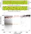 |
Fig. 1 Bursts and drift rates (df /dt) observed with FAST. (a) Representative examples of bursts observed on 2 December. Many linearly drifting discrete bursts show up clearly. About 700 individual bursts were identified and their drift rate measured across the observed frequency range (examples are displayed in red). With FAST, negative Stokes V correspond to LH circular polarisation (Wang et al. 2023). (b) Representative examples of bursts observed on 3 December. Their morphology is quite different from the previous day. About 50 000 individual sub-bursts were identified and their instantaneous drift rate estimated (examples are displayed in light blue). Examples of overall drifts of sub-burst alignments are displayed in orange. (c) Individual burst drifts on 2 December are displayed as diamonds, and their linear dependence versus the frequency is the best fit red line (similar to Paper I). Individual sub-burst drifts on 3 December are displayed as dots below 1150 MHz and ‘+’ above 1290 MHz. Their distribution is much more dispersed than the one on the previous day. The best fit linear trend of df/dt(f) for individual sub-burst is the short-dashed orange line between –350 and –680 MHz. Overall drifts of sub-burst trains or clusters are largely spread between –500 and –1000 MHz/s (lower grey-shaded region) and display a small statistical variation between about –750 MHz at 1000 MHz and –840 MHz at 1150 MHz (long- dashed orange line). Determination of these overall drifts is detailed in Appendix A. The upper grey-shaded region and dashed orange lines are the symmetrical of the lower ones with respect to the df /dt = 0 dotted line. |
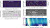 |
Fig. 2 Comparisons of the morphologies of AD Leo’s radio bursts observed on 2 December 2021 (a) and 3 December 2021 (c), with typical Jupiter S-bursts observed at the Nançay Decameter Array (Lamy et al. 2017; Mauduit et al. 2023) (b), and with Solar decameter spike bursts observed with the Huairou/NAOC solar spectrometer (Chernov et al. 2008) (d) and the NenuFAR low-frequency radio telescope (Zarka et al. 2020; Briand et al. 2022) (e). |
3 Physical characteristics and magnetic field of AD Leo
AD Leo (GJ 388) is an M3.5V dwarf with a mass of 0.42 M⊙ and radius of R* ~ 0.4 R⊙ (Mann et al. 2015), located at a distance of 4.9651 ±0.0007 pc from the Solar System (Gaia Collaboration 2021). It has a rotation period of Prot = 2.2300 ± 0.0001 days (Carmona et al. 2023) with an origin (Φ = 0° and longitude Λ = 0° for the direction of the observer) at HJD=2458588.7573; namely, its rotational phase at any HJD can be computed as Φ(°)=(HJD-2458588.7573)×360/Prot mod 360° (and Λ = 360° − Φ). AD Leo’s inclination, namely, angle between its rotation axis and the direction of Earth, is i = 20°, implying an almost pole-on view (Morin et al. 2008). AD Leo is an extensively studied flare star, with an intense magnetic activity revealed by frequent flares (Güdel et al. 2003; Hawley et al. 2003; van den Besselaar et al. 2003; Robrade & Schmitt 2005; Muheki et al. 2020; Namekata et al. 2020).
Prior Zeemann–Doppler imaging (ZDI) studies have suggested that AD Leo has a predominant dipole magnetic field and a nearly pole-on geometry, the magnetic south pole being the visible pole for a terrestrial observer, with magnetic field lines entering into the star (Morin et al. 2008; Lavail et al. 2018). Recent ZDI measurements by SPIRou in late 2020 have revealed to be complicated to interpret: the dipolar component still dominates (~70%) but with significant contributions of higher order terms, especially the large quadrupolar component (~21%), and large residuals of the ZDI modelling of Stokes V profiles (Bellotti et al. 2023). Thus, for purposes such as radio emission modelling, it is considered adequate to use in a first step the purely dipolar fit of AD Leo’s magnetic field, where the field amplitude at the magnetic south pole is 923±70 G, and the dipole misalignment with respect to the rotation axis is 59° ± 2° (Bellotti et al. 2023, Table 1). We note, however, that small-scale field structure likely exists (Yadav et al. 2015; Bellotti et al. 2023), although it should rapidly decrease with the altitude above the photosphere. The long-term evolution of AD Leo’s magnetic field also exists, as demonstrated by Bellotti et al. (2023), which justifies the use of the field description based on ZDI measurements as close as possible in time to FAST observations for our radio emission modelling (configuration 2020b from Bellotti et al. 2023).
Finally, we recall that the analysis of radial velocity measurements led Tuomi et al. (2018) suggesting the existence of a giant planet with a mass of ~0.24 Mjup in spin–orbit resonance (orbital period of 2.23 days). However, this was refuted by subsequent studies, which attributed radial velocity variations to the stellar activity (Carleo et al. 2020; Carmona et al. 2023). A recent study ruled out planets more massive than 27 M⊕ orbiting at the stellar rotation period, as well as planets more massive than 3–6 MJup with periods up to 14 years (Kossakowski et al. 2022).
4 ExPRES analysis of radio burst envelopes
Assuming that the radio bursts from AD Leo detected by FAST are generated via the ECM mechanism at the fundamental of the local cyclotron frequency, we can use the ExPRES code (Exo- planetary and Planetary Radio Emissions Simulator, Louis et al. 2019) to derive constraints on the location and energy of the electrons producing the radio emission. ExPRES was developed for simulating the dynamic spectra of Jupiter’s decameter radio emissions (Hess et al. 2008), and more precisely the t–f occurrence and the sense of circular polarisation of the emissions (not their intensity nor polarisation degree). Inputs to the code include the type of electron distribution driving the ECM (losscone or shell in the velocity space), the characteristic energy of the electrons (in the case of a loss-cone), a magnetic field model at the source (i.e. of Jupiter or, in our case, of AD Leo), the location of the radio sources (e.g. along field lines with fixed longitude that rotate with the planet or star), the thickness of the hollow conical beam produced by the ECM (usually 1°–2°), and the position of the observer (fixed or moving). The code then populates the source field lines with radio sources at the local electron cyclotron frequency (fce = eB/2πm, with B as the amplitude of the local magnetic field and e and m as the charge and mass of the electron, respectively), computes the radio beaming angle at each frequency; namely, the angle relative to the local magnetic field at which the radio emission is beamed (that depends on the frequency and on the electrons energy for loss-cone-driven ECM; it is always 90° for a shell-driven ECM) and compares it to the direction of the observer at each time step. When the difference is less than the beam thickness, the emission is considered detected at the corresponding time and frequency. Emissions produced from a northern magnetic hemisphere are right-hand (RH) circular if on the extraordinary mode (so-called R-X mode), and LH if on the ordinary mode (L-O mode). Opposed senses of polarisation are emitted from a southern magnetic hemisphere. Near-source refraction can be taken into account if a plasma model is available.
In the original ExPRES paper (Louis et al. 2019), the expression of the refraction index and thus of the radio beaming angle were presented in a condensed form and for the R-X mode only. Appendix B of the present paper provides their complete derivation for both R-X and L-O modes (ExPRES Version 1.3.0, Louis et al. 2023).
Following Bellotti et al. (2023), we have considered for AD Leo a magnetic dipole of moment  (i.e. an equatorial surface field of 461.5 G), inclined at 59° from the rotation axis, itself at ~20° from the line of sight, with the magnetic south pole in the hemisphere visible for a terrestrial observer. The star rotates in 2.23 days according to the phase system defined in Sect. 3. The magnetic dipole is assumed to be centred on the star’s centre, and we have not considered the star flattening (negligible for our simulations). Given AD Leo is a relatively cool star, its coronal plasma density likely drops rapidly above the photosphere and the ambient plasma frequency is likely to be smaller than the frequency of FAST observations (≥1 GHz). As a consequence, we neglected near-source refraction and, thus, we assume a straight line propagation from the radio source to the terrestrial observer. This is further discussed in Sect. 6. Figure 3 is a sketch of the geometry of AD Leo’s dipolar magnetic field as seen from a terrestrial observer, with a few radio emission cones displayed.
In Fig. 4, we show typical outputs from ExPRES applied to AD Leo, in which a few selected field lines (of apex distance at magnetic equator 2 R*, i.e. shell parameter L=2, and of longitudes 2°, 10°, 20°, 148°, 150°, 160°, 175°, 180°, 270°, 330° and 350°, as well as the ranges of longitudes 150°–160° and 345°–355° with one field line per degree of longitude) are assumed to radiate at the local fce on the R-X mode from the southern hemisphere. The simulations were performed over 28 hours over 2–3 December, when the radio sources were rotating with the star. The hollow conical beam thickness is assumed to be equal to 1° . Four scenarios were tested, where the ECM is driven by a loss-cone with characteristic energy 5, 10, or 20 keV, or with a shell electron distribution. In each scenario, arcs should be detected by a terrestrial observer in the t–f plane in the frequency range covered by FAST. The envelopes of the radio bursts detected on 2–3 December are displayed as grey-shaded areas at about -03:00 (i.e. ~21:00 on 2 December) and 21:30 to 23:00. For reference, uGMRT detections are indicated as the grey contours. We note that the ExPRES arcs from a single field line displayed in the upper four panels of Fig. 4 have fixed-frequency durations comparable to the envelopes of the observed bursts, whereas emission from a set of field lines spreading over 10° of longitude produce much more extended regions in the t–f plane (lower panel of Fig. 4). This suggests that only a restricted range of stellar field lines were emitting in radio at the time of FAST observations, and not necessarily the same on the two days.
To limit the number of free parameters and make the minimum ad hoc assumptions on the radio source, the modelling presented below assumes an auroral-like emission from AD Leo, where radio emission can be produced at all longitudes. The set of radio-emitting field lines is thus characterised only by its magnetic shell parameter L; namely, the distance of the field line apex to the centre of the star. We consider separately R-X and L-O modes from the northern or southern hemisphere of the star. For a given value of L, we placed radio sources at every degree of longitude along field lines of parameter L and radio waves were assumed to be produced permanently along each entire field line, from the surface of the star to the apex of the field line, at the local fce at each point. The thickness of the hollow cone produced by each point source is assumed to be equal to 1°, to ensure overlapping between the cones produced by consecutive sources separated by 1° of longitude. This results in a quasi-continuous coverage of the parts of the t–f plane where emission should be detected. With this modelling, we thus computed a ‘maximum’ coverage of the t–f plane for each selected L-shell, emission mode, source hemisphere, and ECM energy source.
We have produced simulated dynamic spectra in occurrence and sign of circular polarisation for seven ECM energy sources (loss-cone electron distribution with characteristic electron energy of 5, 10, 30, 100, 200, and 500 keV, and shell electron distribution), and five values of the source L-shell (L=2, 5, 10, 20, and 40 stellar radii), for a terrestrial observer, from 2 December, 20:00 UT, to 3 December, 24:00 UT. This time interval encompasses both observations by FAST. The R- X and L-O modes were simulated from each hemisphere of AD Leo, separately. The criterion used to decide the compatibility of a simulation with the observations is based on whether the envelopes of the radio bursts detected by FAST are included in the t–f region where the simulation predicts emission to occur.
Figure 5 displays significant examples of our ExPRES simulations compared to FAST observations. Panel a of Fig. 5 displays the simulated dynamic spectra for R-X mode produced from AD Leo’s northern magnetic hemisphere by the ECM driven by a loss-cone with characteristic energy 10 keV, for sources placed at every degree of longitude on L-shells 2, 5, 10, 20, and 40 (R*). The part of the t–f plane in which the emission is visible from a terrestrial observer is filled in solid black color, representing RH circular polarisation. The t–f areas in which FAST detected bursts are green-shaded. Green contours refer to uGMRT detections. Panel a shows that the corresponding scenario can account for both detected emissions only for the L=2 magnetic shell. The emission observed on 2 December is compatible with a source at L=2 to L=10, whereas that of 3 December is incompatible with sources at L>2. In addition, R- X mode from the northern magnetic pole produces RH circular polarisation, opposed to the observed one. Panel b displays the simulated dynamic spectra for the same emission mode and scenario but for the southern hemisphere. The predicted emission is displayed in solid red, representing LH circular polarisation. The cases L=2 and L=5 are compatible with both FAST observations; namely, the simulated dynamic spectra include both green areas and the predicted polarisation corresponds to the observed one.
Similar ExPRES simulations for other loss-cone energies and for a shell of electrons are displayed in Fig. C.1. For a 30 keV loss-cone, predicted R-X southern emission is compatible with FAST observations for L=2 to 10 (Panel d of Fig. C.1). The R-X northern emission at L=2 is marginally compatible with the observations, in the sense that the simulated emission includes the observed t–f ranges except the brief extension to 1400 MHz on 3 December (Panel c). For a 100 keV loss-cone, predicted R-X northern emission is incompatible with the observations for all L-shells (Panel e of Fig. C.1), whereas predicted R-X southern emission at L=5 is compatible with the observations (Panel f). For ECM driven by a loss-cone with characteristic energy 200 keV, no simulated dynamic spectrum matches both FAST observations together (Panels g and h of Fig. C.1). Finally, panels i and j of Fig. C.1 display the simulated dynamic spectra for R-X mode produced from AD Leo’s northern and southern magnetic hemispheres by the ECM driven by a shell of electrons. In that case, the emission is beamed at 90° from the magnetic field in the source whatever the electron’s characteristic energy (which is therefore unconstrained). The figure shows that the case L=2 is consistent with FAST observations. Because of the radio beaming angle at 90°, the t–f coverage for shell- driven ECM emission from both hemispheres is identical, but with opposed polarisation.
We have also performed all simulations for the L-O mode, and found that the predicted t–f coverage is identical for R-X and L-O modes from the same hemisphere, but with opposed polarisations. Finally we have checked that doubling the cone thickness (2°) marginally changes the t–f coverages in Fig. 5 and, thus, this does not impact our results. Halving the cone thickness (0.5°) only creates many small gaps in the t–f coverages, such as those in the lower panel of Fig. 4. All ExPRES simulation files (configuration and results) are available from Louis & Zarka (2025).
Table 1 summarises the results of our 7 × 5 × 2 × 2 = 140 ExPRES simulations compared to FAST observations. The predicted t–f coverages are consistent with the observations for loss-cone-driven ECM with 5–100 keV electrons on field lines with L≤5 to 10, on the R-X or L-O mode from the southern magnetic hemisphere. They are also consistent with 5–10 keV loss-cone-driven ECM from the northern magnetic hemisphere, and for shell-driven ECM in both hemispheres, but only on field lines with L=2. When polarisation is taken into account, only R- X mode from the southern hemisphere or L-O mode from the northern hemisphere remain compatible with the observations. The corresponding results are emphasised in boldface style in Table 1.
The height of the radio sources between 1000 and 1500 MHz is between 1.10 and 1.23 R* (for L=2) and between 1.19 and 1.34 R* (for L=10). The latitude of the radio sources is between 40° ± 2° (for L=2) and 69° ± 1° (for L=10).
To test the dependence of our modelling results on AD Leo’s dipolar magnetic field parameters, we have re-computed the plots of Fig. 5 with the 2019b model from Bellotti et al. (2023) (magnetic dipole of moment  inclined at 23° from the rotation axis). The predicted t–f domains covered by ECM emission slightly change, without modifying significantly the conclusions of Table 1. As recent ZDI observations from AD Leo do not suggest any polarisation reversal since 2020, we consider our modelling of Fig. 5 as representative of the situation in late 2021, at the time of FAST observations.
We have also performed ExPRES simulations where magnetic field lines carry radio-emitting electrons only in a restricted longitude range (such as in Fig. 4), to test the possibility of a radio emission induced by the presence of a planet in synchronous orbit, as proposed by Tuomi et al. (2018). We did not find any single restricted longitude range that could account for the emissions observed by FAST on both 2 and 3 December. Thus, in the frame of our simulations (ECM mechanism at the fundamental of the local cyclotron frequency), FAST observations over 2–3 December 2021 cannot be attributed to a star–planet interaction with a planet in synchronous orbit. More generally, the emission from a restricted sector of stellar longitude that would be active on both days is excluded.
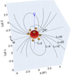 |
Fig. 3 Sketch of AD Leo’s magnetic configuration, based on (Bellotti et al. 2023). The axes (x, y, ɀ) are expressed in stellar radius, R*. The dotted blue line labelled Ω represents the star’s rotation axis (it is displayed at 20° from the line of sight), while the black dotted line labelled M represents the magnetic dipole axis, making an angle of 59° with Ω. Magnetic field lines of L-shell 2-40 are displayed as the solid black lines, for longitudes 20° and 200° (field lines at longitudes 110° and 290° are added for L=2). The auroral ovals (actually circles) at L=2 and fce=1 GHz in both magnetic hemispheres are displayed in orange. Examples of hollow emission cones are shown at the intersection of the ovals and the displayed magnetic field lines at L=2. Cone apices have a brighter orange shading. Cone wall thickness is figured by the orange circles along cone edges. Cones pointing upward (i.e. toward the observer’s hemisphere) can be identified by the field lines visible inside them, whereas cones pointing downward (away from the observer) mask the field lines which carries them. In our simulations, we place the radio sources and emission cones at every degree of longitude. |
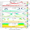 |
Fig. 4 Sample ExPRES simulations of ECM radio emissions from AD Leo between 2 December, 20:00 UT and 3 December, 24:00 UT. Emitting radio sources are placed along AD Leo’s dipolar field lines with magnetic L-shell=2 in the southern hemisphere (in view of the observer), at longitudes indicated on the figure. Emission is produced permanently along each entire field line at the local fce on the R-X mode and beamed in a hollow cone of aperture self-consistently computed by ExPRES (see Appendix B) and of thickness 1°. The upper 4 panels display simulated emissions from a single field line at each indicated longitude. The lower panel displays simulated emissions from two sets of field lines covering each a 10° longitude range with one field line per degree of longitude (the small t–f gaps, that result from this discretisation, disappear with a denser filling, i.e. with more field lines per degree of longitude). Radio arcs are observed across the t–f plane from 0 to 1.7 GHz. Signals observed below ~0.2 GHz result from a mix of emissions produced at various longitudes. Each panel explores one emission scenario for the ECM driver (loss-cone with 5, 10, or 20 keV characteristic energy, or shell in the velocity space). The color scale indicates the beaming angle θ(°) of the emission relative to the local magnetic field vector. Bursts were detected by FAST in the grey-shaded areas, while the grey contours refer to uGMRT detections. |
Comparison of ExPRES simulations with FAST observations: L-shell ranges for which the simulated t–f domain includes the observed bursts.
 |
Fig. 5 Examples of simulated emission envelopes with ExPRES. R- X mode is emitted from the northern (a) or southern (b) hemisphere, by loss-cone-driven ECM with characteristic energy 10 keV. Five dipolar magnetic shells (L=2, 5, 10, 20, 40) are simulated in each case, with active radiosources along all field lines at the corresponding shell (actually, at every degree of longitude; small t–f gaps due to this discretisation have been interpolated). An Earth-based observer detects RH (black) or LH (red) polarised emission depending on the hemisphere of origin and emission mode. In both panels, the bursts were detected by FAST in the green-shaded areas, while the green contours refer to uGMRT detections. |
5 Analytical study of burst drift rates
Fast-drifting bursts provide us with an independent way to estimate the source L-shell and electrons energy. For a dipolar magnetic field, the calculations can be conducted analytically. Following Zarka et al. (1996) and Mauduit et al. (2023), we can write the magnetic field amplitude at distance R from the star’s centre and colatitude ǿ from the magnetic axis as:
 (1)
(1)
with Be the equatorial surface field (here 461.5 G) and R in R* and hence the electron cyclotron frequency fce can be written:
 (2)
(2)
with ƒ = ƒce, and ƒe the cyclotron frequency at the equator at 1 R*, distance. The drift rate dƒ/dt produced by electrons of energy E, moving along a field line L can be written:
 (3)
(3)
with s as the curvilinear abscissa. Using the equation of a dipolar field line
 (4)
(4)
and with ds2 = dR2 + R2dθ2 and ds/dt = υ//, we obtained
 (5)
(5)
with
 (6)
(6)
Assuming that there is no distributed accelerating electric potential nor any potential drop along the source field line (i.e. the electrons are in adiabatic motion), the expression of the parallel electron velocity is deduced from the total energy E (keV), with the help of the conservation of the energy of the electron ( = constant), because the magnetic force does not work, and by expressing the first adiabatic invariant of the electron motion in a variable magnetic field amplitude (
 = constant). We obtain:
 (7)
(7)
with ϕe the equatorial pitch angle of the electron (i.e. ϕe = arcsin(υ⊥/υ) at the magnetic equator), and  with Eo = 511 keV the electron’s energy at rest. We note that the sign of the drift rate depends on that of υ//, which reflects the sense of motion of the electrons along the source field line. Down-going electrons produce positively drifting radio waves (frequency increases with time) whereas up-going electrons produce negatively drifting signals. The modulus of the drift rate does not depend on its sign.
The altitude of the mirror point of an electron, at which υ = υ⊥ , depends only on its equatorial pitch angle:
 (8)
(8)
which implies
 (9)
(9)
where the altitude of the mirror point, at which B = Bmirror, is given by the expression of B(R, θ). Alternately, the equatorial pitch angle on a field line L is expressed as:
 (10)
(10)
The equatorial pitch angle that corresponds to a mirror point at the stellar surface (i.e. at 1 R*) is
 (11)
(11)
with ƒmax the cyclotron frequency at the footprint (R = 1R*) of the field line L. Electrons with ϕe < ϕe1 precipitate into the star and are lost by collisions, generating a loss-cone in the reflected distribution, while electrons with ϕe > ϕe1 have their mirror point above the star’s surface.
Using the above equations we have computed predicted drift rates over the range of FAST observations for electrons with energies of 5–200 keV, moving along field lines with L values of 2–40. Figure 6 displays representative examples at 5, 30, and 100 keV. The modulus of the drift rates is plotted for the different L-shells (displayed in different colors) and for three values of ϕe on each L-shell (see caption of Fig. 6). The drift rates measured by FAST on 2 December are displayed with the thick solid red line, while the overall (resp. sub-burst) drift rates on 3 December are displayed as the long-dashed (resp. short-dashed) orange line, as in Fig. 1c. From Fig. 6 (actually from the entire series of simulations with energies 5–200 keV), we conclude that (i) the drift rates of 2 December are compatible only with electrons of energy 20–30 keV, (ii) the overall drift rates of 3 December are compatible only with electrons of energy 30–100 keV, and (iii) the sub-burst drift rates of 3 December are incompatible with electron adiabatic motion at all energies. Moreover, for energies of 20–30 keV, matching the observed drift rates along field lines with L>10 requires electrons moving quasi-purely parallel to the star’s dipolar field lines (equatorial pitch angle ϕe ≪ 1°), which is quite difficult to achieve from low latitude acceleration, which will necessarily lead to an angular dispersion of electron velocities. If we restrict this to the more plausible range 1° < ϕe < 1.2 × ϕe1, we obtain the domains displayed in Fig. 7 for an electron energy of E=30 keV. Here, we see that observed drift rates can be reached only on field lines with L≤ 10.
Thus, the results of this analysis are quite convergent with those obtained completely independently from the ExPRES simulations in the previous section, especially for R-X southern emissions. Both are consistent with electrons whose energy is about 30 keV, moving adiabatically along field lines with L≤10. Possible L-O northern emission deduced from ExPRES simulations (column ‘L-O North’ of Table 1) corresponds to electron energies lower than those deduced from drift rate calculations. Burst drift rates on 2 December are particularly well matched by 20–30 keV electrons. On 3 December, sub-burst drifts are inconsistent with large scale electron motion along dipolar field lines whatever their energy, while overall drift rates may be consistent with an energy about twice higher than on the previous day.
 |
Fig. 6 Drift rates calculated in FAST range for electrons with energy 5 keV (a), 30 keV (b), and 200 keV (c). On each panel, drift rates for each L value (same values as in Fig. 5) are plotted in a given color (L=2: black, L=5: violet, L=10: blue, L=20: green, L=40: pink). For each L-shell, drift rates are computed for 3 values of the equatorial pitch angle [ϕe1/2, ϕe1, 1.3 × ϕe1], and the curve corresponding to ϕe = ϕe1 is thicker than the other two. The corresponding value of ϕe is indicated next to each curve in the corresponding color. The red and orange lines represent the drift rates measured by FAST (see text). The increased electron energy corresponds to increased drift rates proportional to the electron velocity across the source regions. |
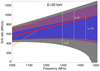 |
Fig. 7 Ranges of calculated drift rates along dipolar field lines with L- shell 2, 5, and 10, for an electron’s energy of 30 keV and equatorial pitch angles between 1° (upper limit of each domain) and 1.2 × ϕe1 (lower limit). The red and orange lines represent the drift rates measured by FAST on 2–3 December (see text). |
6 Discussion and conclusions
As discussed in Paper I, the high flux density (>100 mJy) and brightness temperature (Tb up to 1018 K) of AD Leo’s radio bursts, their high circular polarisation degree V/I, and their fine temporal structure at a few milliseconds timescale suggest that the generation process occurs via the ECM mechanism at the fundamental of the local cyclotron frequency ( f = fce), as for Jovian S-bursts. The latter argument (fine time structure) is especially important, since plasma emission with a fine structure that is much shorter than 1 s is unlikely (Vedantham 2021). Conversely, the very high maser growth rates ensure fast growth possibly up to saturation (Treumann 2006).
We restricted our study to emission at the fundamental of the cyclotron frequency because the corresponding ECM growth rates are generally much larger than for higher harmonics (Treumann 2000, 2006), so that the fundamental should dominate below ~2 GHz unless it is trapped or absorbed in the plasma. The emission at harmonics of fce should also reach much higher frequencies than those observed to date by FAST (Paper I) or by most of the previous observers (Abada- Simon et al. 1994; Osten & Bastian 2006, 2008; Villadsen & Hallinan 2019). Harmonic emission from AD Leo may have been detected in the range 2.8–5 GHz (Stepanov et al. 2001; Villadsen & Hallinan 2019).
Figures 2a and 2b, which offer a qualitative comparison of the morphology of AD Leo’s bursts from 2 December with Jupiter’s S-bursts reveal a striking similarity. The main difference is the sign of the drift rate, which suggests down-going electrons on AD Leo and up-going ones at Jupiter. In Figs. 2c, 2d, and 2e, we also show that the morphology of AD Leo’s bursts from 3 December is reminiscent of that of Solar spikes, also commonly attributed to ECM (Benz 1986; Wu et al. 2007; Chernov et al. 2008). The overall drift of AD Leo’s bursts is negative in that case.
The interpretation of FAST observations from December 2021 favours R-X mode from AD Leo’s southern magnetic hemisphere, because this mode is consistent with both the t–f coverage and the measured LH polarisation. It is also consistent with the fact that the South magnetic hemisphere is more optimally viewed by a terrestrial observer.
This carries an implication in terms of the density of AD Leo’s atmosphere. Fundamental X-mode emission requires fpe/fce < 0.3 (with fpe [kHz]  [cm−3] the plasma frequency) in the radio source region (Melrose et al. 1984; Treumann 2006) in the range of FAST observations; namely, 1– 1.5 GHz. Since AD Leo is a cool red dwarf (Teff ~3500 K, Mann et al. 2015) we can assume (as a first approximation) a corona in hydrostatic equilibrium with a density (and hence an electron density) varying as Ne(ɀ) = N0exp(–ɀ/H) (with ɀ as the altitude above r = 1 R*, and N0 as the coronal base density). For the Sun, the coronal base density is N⊙ ~ 3 × 108 cm−3 and the scale height is H is H⊙ ~ 108 m. For a red dwarf, previous authors have assumed a coronal base density of N* ~ 100 × N⊙ and a scale height of H*, ~ 0.5–1.2 H⊙ (Villadsen & Hallinan 2019). Following Mohan et al. (2024) and Villadsen & Hallinan (2019), we can write the electron density profile in AD Leo’s atmosphere as
![Mathematical equation: ${N_e}(r)\left[ {c{m^{ - 3}}} \right] = n \times {2.510^{10}}\exp \left[ { - (r - 1)/\left( {h \times 0.38{R_ * }} \right)} \right]$](/articles/aa/full_html/2025/03/aa50950-24/aa50950-24-eq19.png) (12)
(12)
where we have introduced the dimensionless parameters n and h characterising the coronal base density and scale height relative to the proposed model (i.e. n = 1 and h = 1 in Villadsen & Hallinan 2019).
With the dipole field of AD Leo allowing us to determine fce (ɀ) along any field line (Eqs. (2) and (4)), we obtained, for the field lines with L-shell 2 to 10, the ratio fpe /fce displayed in Fig. 8 for n ∈ [0.2,0.5,1] and h ∈ [0.2,0.5,1]. We see in Fig. 8 that R-X mode sources at L=2 are very unlikely, unless both n and h are much smaller than 1. Along field lines with L=5 to 10, fundamental R-X mode generation via ECM in the range of 1–1.5 GHz imposes h ~ 0.2 (whatever the value of n), or h up to 0.5 if n ~ 0.2. These parameters correspond to a corona significantly less dense than in Villadsen & Hallinan (2019) at the radio sources altitude (1.10 to 1.34 R*,) and latitude (40° to 69°), imposing constraints on coronal models for M dwarfs.
We have noted that both ExPRES simulations (constrained by the ECM energy source, characteristic electron energy in the case of a loss-cone, and L-shell) and drift rate estimates (determined by the electron energy, L-shell, and electron pitch angle at the equator) have given consistent results, pointing at radiating electrons with an energy E=20–30 keV, moving along field lines with L~2–10. The above plasma density estimates rather favour the range L~5–10. We do not claim a high accuracy on either L or E, but the results are indicative of mid- to high-latitude emissions by moderately energetic electrons. Positive drifts, on 2 December, rather favour shell-driven ECM with down-going electrons (in that case along L~2 field lines), while a loss-cone is compatible with the negative drift rates observed on 3 December. On this latter day, the drift rate calculations suggest that the bursts are either produced by a mechanism different from ECM (the overall drifts being either coincidental or due to an overall source motion at a speed similar to that of electrons in adiabatic motion along dipolar field lines (Willes 2002)); or alternatively, they may be produced via ECM by electrons travelling along magnetic field lines that are not described by a large-scale dipolar field (e.g. smaller scale magnetic loops).
These results, based on two 3 hour observations only, are of course preliminary, but they are a first quantitative analysis, standing as a proof of concept that shows that detailed characterisation of ECM emission regions, electron energies, and coronal plasma density becomes possible using fine structures observed in stellar radio bursts. The small t–f extent of the observed overall t–f patterns being much less extended than our simulations of Fig. 5 suggests that restricted longitude ranges (likely different) are emitting on the two days. More observations, especially clustered in time, will obviously bring better constraints. On a finer timescale, resolved stellar radio bursts also carry information about their magneto-plasma of origin and can be effective diagnostic tools for the emission mechanism and electron acceleration process.
It must be noted that ExPRES simulations and drift rate calculations benefit from the knowledge acquired on ECM operation in Solar System planetary magnetospheres (Zarka 1998; Treumann 2006). For example, the quasi-periodicity at ~5 Hz of burst occurrence on 2 December 2021 suggests intermittent electron acceleration. At Jupiter, similar bursts (Fig. 2) were interpreted as due to electrons accelerated by Alfvén waves of frequency 5–20 Hz, excited along Jupiter’s magnetic field lines by its moon Io, and amplified at the feet of these field lines in the so-called ionospheric Alfvén resonator (Hess et al. 2007; Mauduit et al. 2023). Alfvén waves have also been invoked in the case of Solar spikes (Wu et al. 2007). Radio burst observations may thus eventually constrain the Alfvén speed (VA = c(fce/fpe)(me/mp)1/2, with c as the speed of light and me and mp as the masses of the electron and proton, respectively) at the base of the corona.
Based on the above conclusions, we may speculate a little further about the large-scale physical driver of AD Leo’s radio bursts; in particular, we consider whether they result from the flare paradigm (see e.g., Zic 2020) or from the planetary magnetosphere paradigm (see e.g., Hallinan et al. 2015). The flare paradigm leaves room for ECM emission as long as adequate fpe/fce ratios exist in the source region (Morosan et al. 2015, 2016; Yu et al. 2024). The similarity of the spikes from 3 December with Solar spikes (Fig. 2) rather supports this paradigm, although no evident correlation was noted in Paper I between optical and radio flares. However, we note that optical flares might be too small to be detected by the optical telescopes used in Paper I, or they could happen before the radio flares and inject accelerated electrons into the large-scale magnetic field, whose radio signature would occur after some accumulation (e.g., Yu et al. 2024). In the planetary magnetosphere paradigm, the main question is the source of electron acceleration (or of the Alfvén waves that cause it). Usual suspects are corotation breakdown and star-planet interaction with a planetary companion. We discussed in Sects. 3 and 4 the unlikeliness of an adequate planetary companion for AD Leo and that is the reason why we did not explore it via ExPRES simulations beyond the synchronous orbit (this would have involved too many free parameters). Further observations may lead us to reconsider this possibility. We are thus left with corotation breakdown (Nichols 2012; Turnpenney et al. 2017) and with the fact that we located the radio sources along field lines of relatively low L; namely, likely to be in the sub-Alfvénic region of the stellar corona. Considering the more massive wind of red dwarfs and the faster rotation (by ~13 times) of the star compared to the Sun’s, we propose that electron acceleration driving ECM on sets of field lines in restricted longitude sectors may be caused by corotation breakdown applied to plasma blobs in the inhomogeneous stellar wind, occurring at a few R*, from the star. This is similar to what happens at Jupiter in the external regions of the Io plasma torus (Yang et al. 1994; Louarn et al. 1998).
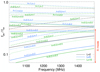 |
Fig. 8 fpee/fce values in the frequency range of FAST observations, for a dipolar magnetic field of moment |

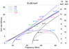 |
Fig. 9 Drift rates similar to Fig. 6 but calculated in NenuFAR’s frequency range, for an electron energy of 30 keV. The curves are globally shifted vertically by a change of electron energy; hence, the different vertical scales on the right side corresponding to different electron energies of 10 and 50 keV. |
7 Perspectives
With the start of operations of the large sensitive low-frequency array NenuFAR in France, in the range 10–85 MHz (Zarka et al. 2020), low-frequency observations of AD Leo’s radio bursts might bring complementary constraints to those obtained at higher frequencies with FAST.
In support of such observations, which were actually initiated in 2023, we have extrapolated the data in Fig. 6 to the spectral range of NenuFAR to estimate the magnitude of the drift rates that should be searched for (displayed in Fig. 9). Surprisingly, we find drift rates of order of 10 MHz/s, very similar to those of Jupiter S-bursts in the same spectral range. We note that cyclotron frequencies matching the lowest frequencies of the NenuFAR range cannot be reached in AD Leo’s environment on field lines with L<5 (fpe≥ 20 MHz along L=4, fce ≥ 48 MHz along L=3, and fce ≥ 85 MHz along L=2).
Similarly, we have extrapolated Fig. 8 in the spectral range of NenuFAR and obtained Fig. 10. If the hydrostatic description of AD Leo’s atmosphere holds up to a few R*, distance, low values of fpe /fce would be possible, thereby allowing for fundamental R-X mode ECM emission (identified through its circular polarisation sense) in the low-frequency source region for a relative coronal scale height twice as low as that reported in Villadsen & Hallinan (2019) (h ≤ 0.5).
Therefore, observations of emission occurrence and drift rates at low radio frequencies would be very powerful for better locating the sources and estimating electrons’ energies. Coordinated high- and low-frequency observations are also potentially very informative, as Fig. 4 shows that due to the ECM beaming, combined with the stellar rotation, emission from the same field line at different frequencies is expected to be received on Earth with a delay of up to several hours. The measured delay will be a very strong constraint on the fit to ExPRES simulations. Of course, contemporaneous ZDI maps will be of utmost importance to apply ExPRES to reliable magnetic field topologies.
Acknowledgements
P.Z. and C.L. acknowledge funding from the ERC under the European Union’s Horizon 2020 research and innovation program (grant agreement Nº 101020459-Exoradio). J.Z. and H.T. are supported by NSFC grant 12250006. This work made use of the data from FAST (Five-hundred-meter Aperture Spherical radio Telescope). FAST is a Chinese national mega-science facility, operated by National Astronomical Observatories, Chinese Academy of Sciences.
Appendix A Drift rates of sub-bursts and sub-burst trains on 3 December 2021
On 2 December, drift rates of linear t–f structures were easily measurable. Figure 3a of Paper I and Fig. 1c of the present paper showed the clear dependence of df /dt on the frequency, varying from +550 MHz/s at 1000 MHz to +970 MHz/s at 1470 MHz.
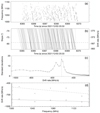 |
Fig. A.1 Example of determination of the overall drift rate of sub-burst trains on 3 December 2021. (a) Five seconds of catalogued sub-bursts reproduced from Fig. 8c of Paper I. (b) Result of parametric linear de-dispersion and spectral integration of (a), as a function of slope (left scale) or drift rate (right scale). The dashed horizontal line about -500 MHz/s indicates the drift rate for which most of the burst clusters of (a) align. (c) Standard deviation of each line of (b) (actually exponential of values of (b) are used to enhance the contrast). The dashed vertical line indicates the peak value, obtained at −514 MHz/s. (d) Distribution of overall drift rates computed in 20 s × 30 MHz intervals between 1000 and 1150 MHz. For each of the 5 frequency intervals, the diamond indicates the average overall drift rate and the ‘+’ the 10 % and 90% quantiles of their distribution. The solid line is the linear fit of the average values, and the dashed lines those of the quantiles. The lower values about -1000 MHz/s are ‘saturated’ by the time resolution of the original dynamic spectrum (a), which prevents us from distinguishing clearly between drift rates steeper than -1000 MHz/s; we thus limited our parametric de-dispersion to that value. |
On 3 December, the morphology of the bursts, very different from the previous day, was blob- or spot-like as shown in Fig. 1b, reminiscent of some solar radio spikes (Benz 1986; Wu et al. 2007; Chernov et al. 2008) (see also Figs. 2c, 2d, and 2e). About 50000 individual sub-bursts were catalogued, with drift rates from −5000 to +3300 MHz/s (dots and ‘+’ in Fig. 1c). The linear fit of df /dt(f) leads to the short-dashed orange line in Figs. 1, 6 and 7, which is not compatible with electron’s adiabatic motion in a large-scale dipolar magnetic field (cf. Figs. 6 and 7). However, in Paper I, sub-burst alignments or clusters were clearly identified, as illustrated in Figs. 1b and A.1a (the latter reproduces Fig. 8c of Paper I).
To quantify the overall drifts of these clusters, we performed a re-analysis of the sub-burst catalogue. This catalogue contains for each sub-burst its t–f position and linear shape as well as its intensity and polarisation. Figure A.1a displays the corresponding sub-bursts detected in the same interval as Fig. 8c of Paper I. To obtain an estimate of the overall drift of sub-burst trains, we ‘dedispersed’ the dynamic spectrum as is done for pulsar pulses (e.g., Zakharenko et al. 2013), but correcting for a linear drift, instead of one in 1/ f2 drift for pulsars (i.e. for each trial drift rate df /dt, we shifted each time series at frequency f relative to a reference frequency f0 by δt = df /dt × (f0 − f)). We then integrated the de-dispersed signal to obtain a time series for each trial drift rate. The result of this operation is displayed in Fig. A.1b as a function of time and slope or drift rate. In the 5 s example displayed, the overall drift rate clearly peaks around −500 MHz/s (horizontal dashed line), where most caustics appear in the t − df /dt plane. To determine automatically the best drift rate, we computed the standard deviation of the time series obtained for each trial drift rate, displayed in Fig. A.1c (where we have taken the exponential of the values in Fig. A.1b to enhance the contrast of the result). It peaks for the drift rate that aligns best the sub-burst clusters (here, equal to −514 MHz/s, shown as a vertical dashed line). We performed this analysis in frequency intervals of 30 MHz and time slices of 20 s over the entire observation of 3 December. In each frequency interval, we computed the average overall drift rate and the 10% and 90% quantiles of their distribution, plotted in Fig. A.1d. The variation of the 10% and 90% quantiles (dashed) define the lower grey-shaded area in Fig. 1c and the variation of the average overall drift rate with frequency (solid line) is the long-dashed orange line in Figs. 1, 6 and 7.
Appendix B General derivation of the ECM radio beaming angle θ for the R-X and L-O modes
We detail here how to derive the dispersion equation in a cold magnetised plasma, and its solution as a function of θ, the angle between the local magnetic field B and the wave vector k.
Appendix B.1 Dispersion equation
To obtain the dispersion equation in a cold magnetised plasma, we use the following Maxwell equations (Maxwell 1865): the Maxwell-Amperes relationship:
 (B.1)
(B.1)
the Maxwell-Faraday relationship:
 (B.2)
(B.2)
the current density formula:
 (B.3)
(B.3)
and that of the dielectric tensor:
 (B.4)
(B.4)
We will also use the fact that solutions are in the form of plane waves, and that all the quantities f (r, t) are proportional to ei(k.r−ωt). That gives us:
 (B.5)
(B.5)
The refractive index N of a medium is defined as the ratio of the speed of light in a vacuum c to the phase velocity vф of a wave propagating in the medium. In the case of a plane wave, the phase velocity corresponds to the propagation speed of the wavefront along the wave vector k, i.e.  . Therefore,
  .
.
The magnetic field B (of unit vector b) is directed along ez. The wave vector k is contained in the plane (ex, ez). Theses two vectors form an angle θ. In this reference system, we can define N = (N sinθ, 0, N cosθ).
We therefore obtain:
 (B.6)
(B.6)
For deriving KE, we start from the equation of motion:
![Mathematical equation: ${\mathop \sum \nolimits^ ^}F = m{{\partial \v } \over {\partial t}} = e[E + \v \times B],$](/articles/aa/full_html/2025/03/aa50950-24/aa50950-24-eq28.png) (B.7)
(B.7)
giving us:
![Mathematical equation: ${m_s}{{\partial {\v _s}} \over {\partial t}} = {e_s}\left[ {{E_{\bf{1}}} + {\v _{s{\bf{1}}}} \times {B_0}} \right],$](/articles/aa/full_html/2025/03/aa50950-24/aa50950-24-eq29.png) (B.8)
(B.8)
with s standing for ‘species’ (ion or electron), E = E0 + E1 = E1, vs = v0 + vs1 = vs1 (cold plasma), B = B0 + B1, and vs1 × B1 = O2(ϵ) (second order, very low in front of first order).
As we are assuming the solutions are in the form of plane wave, by projecting along x, y and z, we obtain:
 (B.9)
(B.9)
With  the cyclotron pulsation for each species. Hence
 (B.10)
The current density is expressed as
 (B.11)
from which we obtain the conductivity tensor σ:
 (B.12)
Then we can express the dielectric tensor:
 (B.13)
which is therefore written:
 (B.14)
where S, P and D correspond to the Stix notation (Stix 1962):
 (B.15)
Finally:
 (B.16)
The determinant of this matrix gives an N-squared equation of the form:
 (B.17)
with
 (B.18)
In the oblique propagation (i.e. θ ≠ 0° or 90°), the solutions are given by:
 (B.19)
The solutions of this dispersion equation give a relation between the refractive index N, the wave gyrofrequency ω and the angle θ between the wave vector and the ambient magnetic field.
The ± sign indicates the existence of two branches to the solutions. To understand the meaning of this ± for the wave, we derive in the next section the Altar-Appleton-Hartree expression of the refractive index.
Appendix B.2 Altar-Appleton-Hartree expression
To find the solution to this determinant directly in Altar-Appleton-Hartree form, it is easier to put N2 = 1 + ξ and solve
 (B.20)
The solutions of this equation are given by:
 (B.21)
In the following, we used the approximation that at high frequencies, the terms relating to the ions in the expression of S, P, and D are negligible because mi≫ me and, therefore, ωpi≪ ωpe, as well as ωci≪ ωce
To finally arrive at the Altar-Appleton-Hartree equation, each term in the above equation must be rewritten, factoring by  .In the end, this gives us
 (B.22)
As mentioned earlier, the ± sign indicates the existence of two branches to the solutions. These branches (represented in Fig. B.1) are framed by cutoff and resonance frequencies and named as follow:
+ :whistler mode (ω < ωp);
Left-Ordinary (LO) mode (ω > ωp).
− : Left-eXtraordinary (LX) mode (ωL < ω < ωp);
Right-eXtraordinary(RX)-Z mode (ωp < ω < ωUH);
RX mode (ω > ωR).
We note that below ωce, in oblique and parallel propagatin (so for θ < 90°), the naming of the branches of the Appleton-Hartree equation for the right and left modes depends on the value of the frequency, as there is a discontinuity at ω = ωpe, which implies a change of sign in the equation. Therefore:
for ω > ωce → NR = N+ and NL = N−,
for ωce > ω > ωpe → NR = N− and NL = N+,
for ωpe > ω → NR = N+ and NL = N−,
meaning that in-between ωpe and ωce there is an inversion of the branches to the solutions for the right and left modes (this is taken into account in Fig. B.1).
In Fig. B.1, we see that only L-O and R-X modes tend to N = 1 and therefore tend towards a high-frequency light wave. These modes are therefore capable of propagating in the vacuum outside of the plasma. It is these two modes that we simulate in ExPRES.
Appendix B.3 Solution of the dDispersion equation function of θ in the oblique case (loss-cone distribution function)
We now want the solution of the dispersion equation (see Eq. B.19), but only function of θ, the angle between the ambient magnetic field, B, and the wave vector, k, as this is what we compute numerically, and in a self-consistent way, in the ExPRES code.
Appendix B.3.1 Equation of the Electron Cyclotron Maser instability in the oblique case (loss-cone distribution function)
In the Electron Cyclotron Maser Instability case, the oblique propagation is obtained when the instability is driven by a loss-cone electron distribution function. The wave-particle resonance equation for the Electron Cyclotron Maser Instability is expressed as
 (B.23)
where ωce is the electron cyclotron angular frequency, ‖ refers to the parallel component of the wave vector k and of the velocity, vr, of the resonant (r) electrons, and Γr is the Lorentz factor associated with the gyration motion of these electrons:
 (B.24)
We recall that the aperture of the conical emission sheet θ is defined by the angle between the magnetic field vector and the wave vector. The magnetic field B (of unit vector b) is directed along ez. The wave vector k is contained in the plane (ex, ez). Assuming that the emission pattern has a cylindrical symmetry of revolution around the magnetic field line, the angle θ can be defined as
 (B.25)
In the weakly relativistic case, the resonance equation is a circle in velocity space:
 (B.26)
 (B.27)
 (B.28)
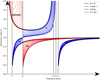 |
Fig. B.1 Refractive Index, N, as a function of the frequency f (with ω = 2πf ) for a low-density plasma (i.e., fce > fpe, required for the ECM to occur). The red areas corresponds to the + branch of the Appleton-Hartree expression, while the blue area correspond to the - branch. The oblique propagation dispersion curves for different θ are shown as thin coloured lines (with δθ = 5°), while dispersion curves for parallel propagation (θ = 0°) are shown as thick black lines, and those for perpendicular propagation (θ = 90°) as thick black dashed lines. The frequencies of the L-mode cutoff fL, plasma cutoff fpe , cyclotron resonance fce , upper hybrid resonance fUH and R-mode cutoff fR , are indicated on the x-axis. In this example, fce/ fpe = 0.3. In reality, it is lower than that, but it has been enlarged here for the sake of readability. |
From Equations B.25 and B.27, and by inserting the refractive index of the medium, written as
 (B.29)
v0 can be rewritten as follows:
 (B.30)
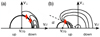 |
Fig. B.2 Electron distribution functions able to amplify radio waves. (a) In a shell-type distribution, the ∇υ⊥ positive gradient of the distribution function is located along the inner edge of the distribution (red arrows). The ECM resonance circle leading to amplification is tangent to it and centred at υ‖0 = 0. (b) In a loss-cone distribution, the loss-cone is a region depleted in electrons, lost by collision with the atmosphere. This region is located below the dashed line, defined by the pitch angle α. The largest positive gradient ∇υ⊥ of the distribution function (red arrow) is along the edge of the loss-cone, at some resonance velocity υr. The ECM resonance circle leading to maximum amplification is tangent to this gradient, and is centred on υ‖0 = υr / cosα. The figure is reproduced from Hess et al. (2008). |
For loss-cone-type electron distributions, the resonance circle (Fig. B.2b) is centred on a non-zero velocity υ0 (see Eqs. B.27 and B.30), which produces an oblique emission (k‖ , 0) with respect to the magnetic field (see Eq. B.23). The position of the resonance circle is related to the angle of the loss-cone α, as shown in Fig. B.2b. This pitch angle defines the position of the mirror point (the point where υ‖ = 0):
 (B.31)
with  the cyclotron pulsation at the mirror point, i.e. here at the altitude of the peak of the UV aurora. Jupiter’s UV aurorae are indeed the result of the collision between the energetic electrons (associated with the radio emissions considered here) and the neutral atmosphere. Their altitude is therefore a good approximation of the limit mirror point, beyond which the electrons are lost in the atmosphere, producing the cone of loss visible in Fig. B.2b.
Appendix B.3.2 Determination of the solution of the dispersion equation function of θ
As we want the solution of the dispersion equation (see Eq. B.19), but only as a function of θ, we therefore go back to Eq. B.17. So we first express the refractive index N specific to the loss-cone electron distribution function.
For that, we use several equations: Eq. B.30 which describes the centre, υ0, of the resonant circle as a function of N and θ; the expression of the resonant electron energy υr and υ0 as a function of the pitch angle α (that describes the position of the mirror point where υ‖ = 0):
 (B.32)
(see Fig. B.2a for resonant electrons) and finally, using the fact that υr << c (which is true for electron energies of a few keV to ∼30 keV) , we can express the value of ω for oblique emissions only as a function of υr :

 (B.33)
This gives for N :
 (B.34)
Using the dispersion relation (Eq. B.17) and the equation above, we can rewrite it as:
 (B.35)
Thus, using the definitions of Eq. B.18:
 (B.36)
with the definitions of S, P, and D given in Eq. B.15 page 14, the dispersion relation can be expressed as a function of θ as the only unknown:
 (B.37)
with sin2 θ = 1 − cos2 θ,
 (B.38)
Finally, Eq. B.35 can be rewritten as follows:
![Mathematical equation: $\eqalign{ & \Leftrightarrow \left[ {P\left( {{S^2} - {D^2}} \right) - {\chi ^2}\left( {{D^2} - {S^2} + PS} \right)} \right]{\cos ^4}\theta + \left[ {{\chi ^4}(P - S) + {\chi ^2}\left( {{D^2} - {S^2} - PS} \right)} \right]{\cos ^2}\theta + {\chi ^4}S = 0, \cr & \Leftrightarrow a{\cos ^4}\theta + b{\cos ^2}\theta + c = 0. \cr} $](/articles/aa/full_html/2025/03/aa50950-24/aa50950-24-eq64.png) (B.39)
(B.39)
Therefore, the solutions of this equation are given by:
 (B.40)
with:
 (B.41)
As for the solutions of N, the ± sign indicates that there are two branches to this equation. As the loss-cone-driven ECM amplify waves only at frequencies f > fce, and as only L-O and R-X modes tend to N = 1 and are therefore capable of propagating in the vacuum outside of the plasma, our only two solutions are:
- +
: LO,
- −
: RX.
The calculation of the beaming angle in L-O or R-X mode is available from Version 1.3.0 in (Louis et al. 2023), the version used in this article.
We note that for ECM loss-cone type simulations that would be done for an observer in the source of radio emissions, at a frequency between fce and fUH ( fce < f < fUH), ExPRES is also able to simulate emissions on the Z mode.
Appendix C ExPRES simulations
Figure C.1 displays representative examples of simulated R-X emission envelopes with ExPRES, for loss-cone-driven ECM with several characteristic energies and for shell-driven ECM. Panels (a) and (b) are identical to Fig. 5.
 |
Fig. C.1 Representative examples of simulated emission envelopes with ExPRES. R-X mode is emitted from the northern (a,c,e) or southern (b,d,f) hemisphere, by loss-cone-driven ECM with characteristic energy 10 keV (a,b), 30 keV (c,d), and 100 keV (e,f). Five dipolar magnetic shells (L=2, 5, 10, 20, 40) are simulated in each case, with active radio sources along all field lines at the corresponding magnetic shell (actually at every degree of longitude; small t–f gaps due to this discretisation have been interpolated). An Earth-based observer detects RH (black) or LH (red) polarised emission depending on the hemisphere of origin and emission mode. On all panels, bursts were detected by FAST in the green-shaded areas, while the green contours refer to uGMRT detections. |
 |
Fig. C.2 (continued) for loss-cone-driven ECM with characteristic energy 200 keV (g,h), and for shell-driven ECM (i,j). |
References
- Abada-Simon, M., Lecacheux, A., Louarn, P., et al. 1994, A&A, 288, 219 [NASA ADS] [Google Scholar]
- Abada-Simon, M., Lecacheux, A., Aubier, M., & Bookbinder, J. A. 1997, A&A, 321, 841 [NASA ADS] [Google Scholar]
- Aschwanden, M. J. 2006, Space Sci. Rev., 124, 361 [Google Scholar]
- Bellotti, S., Morin, J., Lehmann, L. T., et al. 2023, A&A, 676, A56 [NASA ADS] [CrossRef] [EDP Sciences] [Google Scholar]
- Benz, A. O. 1986, Sol. Phys., 104, 99 [NASA ADS] [CrossRef] [Google Scholar]
- Briand, C., Cecconi, B., Chrysaphi, N., et al. 2022, URSI Radio Sci. Lett., 4, 17 [NASA ADS] [Google Scholar]
- Callingham, J. R., Pope, B. J. S., Kavanagh, R. D., et al. 2024, Nat. Astron., 8, 1359 [NASA ADS] [CrossRef] [Google Scholar]
- Carleo, I., Malavolta, L., Lanza, A. F., et al. 2020, A&A, 638, A5 [NASA ADS] [CrossRef] [EDP Sciences] [Google Scholar]
- Carmona, A., Delfosse, X., Bellotti, S., et al. 2023, A&A, 674, A110 [NASA ADS] [CrossRef] [EDP Sciences] [Google Scholar]
- Chernov, G. P., Yan, Y., Fu, Q., Tan, C., & Wang, S. 2008, Sol. Phys., 250, 115 [NASA ADS] [CrossRef] [Google Scholar]
- Gaia Collaboration (Smart, R. L., et al.) 2021, A&A, 649, A6 [EDP Sciences] [Google Scholar]
- Gudel, M., Benz, A. O., Bastian, T. S., et al. 1989, A&A, 220, L5 [NASA ADS] [Google Scholar]
- Güdel, M., Audard, M., Kashyap, V. L., Drake, J. J., & Guinan, E. F. 2003, ApJ, 582, 423 [Google Scholar]
- Hallinan, G., Littlefair, S. P., Cotter, G., et al. 2015, Nature, 523, 568 [NASA ADS] [CrossRef] [Google Scholar]
- Hawley, S. L., Allred, J. C., Johns-Krull, C. M., et al. 2003, ApJ, 597, 535 [Google Scholar]
- Hess, S., Mottez, F., & Zarka, P. 2007, J. Geophys. Res. (Space Phys.), 112, A11212 [NASA ADS] [Google Scholar]
- Hess, S., Cecconi, B., & Zarka, P. 2008, Geophys. Res. Lett., 35, L13107 [NASA ADS] [CrossRef] [Google Scholar]
- Hess, S., Zarka, P., Mottez, F., & Ryabov, V. B. 2009, Planet. Space Sci., 57, 23 [CrossRef] [Google Scholar]
- Jiang, P., Tang, N.-Y., Hou, L.-G., et al. 2020, Res. Astron. Astrophys., 20, 064 [CrossRef] [Google Scholar]
- Klein, K.-L., Salas Matamoros, C., Hamini, A., & Kollhoff, A. 2024, A&A, 690, A382 [NASA ADS] [CrossRef] [EDP Sciences] [Google Scholar]
- Kossakowski, D., Kürster, M., Henning, T., et al. 2022, A&A, 666, A143 [NASA ADS] [CrossRef] [EDP Sciences] [Google Scholar]
- Lamy, L., Zarka, P., Cecconi, B., et al. 2017, in Planetary Radio Emissions VIII, eds. G. Fischer, G. Mann, M. Panchenko, & P. Zarka, 455 [Google Scholar]
- Lang, K. R., & Willson, R. F. 1986, ApJ, 305, 363 [NASA ADS] [CrossRef] [Google Scholar]
- Lang, K. R., Bookbinder, J., Golub, L., & Davis, M. M. 1983, ApJ, 272, L15 [NASA ADS] [CrossRef] [Google Scholar]
- Lavail, A., Kochukhov, O., & Wade, G. A. 2018, MNRAS, 479, 4836 [NASA ADS] [CrossRef] [Google Scholar]
- Louarn, P., Roux, A., Perraut, S., Kurth, W., & Gurnett, D. 1998, Geophys. Res. Lett., 25, 2905 [NASA ADS] [CrossRef] [Google Scholar]
- Louis, C. K., & Zarka, P. 2025, ExPRES AD Leonis Radio Emission Simulations Data Collection (Version 1.0) [Data set] [Google Scholar]
- Louis, C. K., Hess, S. L. G., Cecconi, B., et al. 2019, A&A, 627, A30 [NASA ADS] [CrossRef] [EDP Sciences] [Google Scholar]
- Louis, C. K., Hess, S. L. G., Cecconi, B., et al. 2023, Exoplanetary and Planetary Radio Emission Simulator (ExPRES) [Google Scholar]
- Mann, A. W., Feiden, G. A., Gaidos, E., Boyajian, T., & von Braun, K. 2015, ApJ, 804, 64 [Google Scholar]
- Mauduit, E., Zarka, P., Lamy, L., & Hess, S. L. G. 2023, Nat. Commun., 14, 5981 [CrossRef] [Google Scholar]
- Maxwell, J. C. 1865, Philos. Trans. Roy. Soc. Lond. Ser. I, 155, 459 [NASA ADS] [Google Scholar]
- Melrose, D. B., Hewitt, R. G., & Dulk, G. A. 1984, J. Geophys. Res., 89, 897 [CrossRef] [Google Scholar]
- Mohan, A., Mondal, S., Wedemeyer, S., & Gopalswamy, N. 2024, A&A, 686, A51 [NASA ADS] [CrossRef] [EDP Sciences] [Google Scholar]
- Morin, J., Donati, J. F., Petit, P., et al. 2008, MNRAS, 390, 567 [Google Scholar]
- Morosan, D. E., Gallagher, P. T., Zucca, P., et al. 2015, A&A, 580, A65 [NASA ADS] [CrossRef] [EDP Sciences] [Google Scholar]
- Morosan, D. E., Zucca, P., Bloomfield, D. S., & Gallagher, P. T. 2016, A&A, 589, L8 [NASA ADS] [CrossRef] [EDP Sciences] [Google Scholar]
- Morosan, D. E., Carley, E. P., Hayes, L. A., et al. 2019a, Nat. Astron., 3, 452 [Google Scholar]
- Morosan, D. E., Kilpua, E. K. J., Carley, E. P., & Monstein, C. 2019b, A&A, 623, A63 [NASA ADS] [CrossRef] [EDP Sciences] [Google Scholar]
- Muheki, P., Guenther, E. W., Mutabazi, T., & Jurua, E. 2020, A&A, 637, A13 [NASA ADS] [CrossRef] [EDP Sciences] [Google Scholar]
- Namekata, K., Maehara, H., Sasaki, R., et al. 2020, PASJ, 72, 68 [NASA ADS] [CrossRef] [Google Scholar]
- Nan, R., Li, D., Jin, C., et al. 2011, Int. J. Mod. Phys. D, 20, 989 [Google Scholar]
- Nichols, J. D. 2012, MNRAS, 427, L75 [NASA ADS] [Google Scholar]
- Osten, R. A., & Bastian, T. S. 2006, ApJ, 637, 1016 [NASA ADS] [CrossRef] [Google Scholar]
- Osten, R. A., & Bastian, T. S. 2008, ApJ, 674, 1078 [NASA ADS] [CrossRef] [Google Scholar]
- Prangé, R., Pallier, L., Hansen, K. C., et al. 2004, Nature, 432, 78 [CrossRef] [Google Scholar]
- Robrade, J., & Schmitt, J. H. M. M. 2005, A&A, 435, 1073 [NASA ADS] [CrossRef] [EDP Sciences] [Google Scholar]
- Ryabov, V. B., Zarka, P., Hess, S., et al. 2014, A&A, 568, A53 [NASA ADS] [CrossRef] [EDP Sciences] [Google Scholar]
- Stepanov, A. V., Kliem, B., Zaitsev, V. V., et al. 2001, A&A, 374, 1072 [NASA ADS] [CrossRef] [EDP Sciences] [Google Scholar]
- Stix, T. H. 1962, The Theory of Plasma Waves (New York: McGraw-Hill) [Google Scholar]
- Treumann, R. A. 2000, Geophys. Monogr. Ser., 119, 13 [NASA ADS] [Google Scholar]
- Treumann, R. A. 2006, A&A Rev., 13, 229 [NASA ADS] [CrossRef] [Google Scholar]
- Tuomi, M., Jones, H. R. A., Barnes, J. R., et al. 2018, AJ, 155, 192 [NASA ADS] [CrossRef] [Google Scholar]
- Turnpenney, S., Nichols, J. D., Wynn, G. A., & Casewell, S. L. 2017, MNRAS, 470, 4274 [Google Scholar]
- van den Besselaar, E. J. M., Raassen, A. J. J., Mewe, R., et al. 2003, A&A, 411, 587 [NASA ADS] [CrossRef] [EDP Sciences] [Google Scholar]
- Vedantham, H. K. 2021, MNRAS, 500, 3898 [Google Scholar]
- Villadsen, J., & Hallinan, G. 2019, ApJ, 871, 214 [Google Scholar]
- Wang, P. F., Han, J. L., Xu, J., et al. 2023, Res. Astron. Astrophys., 23, 104002 [Google Scholar]
- Willes, A. J. 2002, J. Geophys. Res. (Space Phys.), 107, 1061 [NASA ADS] [Google Scholar]
- Wu, D. J., Huang, J., Tang, J. F., & Yan, Y. H. 2007, ApJ, 665, L171 [NASA ADS] [CrossRef] [Google Scholar]
- Yadav, R. K., Christensen, U. R., Morin, J., et al. 2015, ApJ, 813, L31 [Google Scholar]
- Yang, Y. S., Wolf, R. A., Spiro, R. W., Hill, T. W., & Dessler, A. J. 1994, J. Geophys. Res., 99, 8755 [NASA ADS] [CrossRef] [Google Scholar]
- Yu, S., Chen, B., Sharma, R., et al. 2024, Nat. Astron., 8, 50 [Google Scholar]
- Zakharenko, V. V., Vasylieva, I. Y., Konovalenko, A. A., et al. 2013, MNRAS, 431, 3624 [NASA ADS] [CrossRef] [Google Scholar]
- Zarka, P. 1998, J. Geophys. Res., 103, 20159 [Google Scholar]
- Zarka, P., Farges, T., Ryabov, B. P., Abada-Simon, M., & Denis, L. 1996, Geophys. Res. Lett., 23, 125 [NASA ADS] [CrossRef] [Google Scholar]
- Zarka, P., Denis, L., Tagger, M., et al. 2020, in URSI General Assembly, session J01: New Telescopes on the Frontier [Google Scholar]
- Zhang, J., Tian, H., Zarka, P., et al. 2023, ApJ, 953, 65 [NASA ADS] [CrossRef] [Google Scholar]
- Zhang, J., Tian, H., Zarka, P., et al. 2024, ApJ, 969, 73 [NASA ADS] [CrossRef] [Google Scholar]
- Zic, A. J. 2020, PhD thesis, University of Sydney, Australia [Google Scholar]
RH circular polarisation was mentioned in Paper I, but it has been corrected after comparison with pulsars with known circular polarisation and after checking the definition of the polarisation measured with FAST (Wang et al. 2023). An erratum has been published (Zhang et al. 2024).
All Tables
Comparison of ExPRES simulations with FAST observations: L-shell ranges for which the simulated t–f domain includes the observed bursts.
All Figures
|
Fig. 1 Bursts and drift rates (df /dt) observed with FAST. (a) Representative examples of bursts observed on 2 December. Many linearly drifting discrete bursts show up clearly. About 700 individual bursts were identified and their drift rate measured across the observed frequency range (examples are displayed in red). With FAST, negative Stokes V correspond to LH circular polarisation (Wang et al. 2023). (b) Representative examples of bursts observed on 3 December. Their morphology is quite different from the previous day. About 50 000 individual sub-bursts were identified and their instantaneous drift rate estimated (examples are displayed in light blue). Examples of overall drifts of sub-burst alignments are displayed in orange. (c) Individual burst drifts on 2 December are displayed as diamonds, and their linear dependence versus the frequency is the best fit red line (similar to Paper I). Individual sub-burst drifts on 3 December are displayed as dots below 1150 MHz and ‘+’ above 1290 MHz. Their distribution is much more dispersed than the one on the previous day. The best fit linear trend of df/dt(f) for individual sub-burst is the short-dashed orange line between –350 and –680 MHz. Overall drifts of sub-burst trains or clusters are largely spread between –500 and –1000 MHz/s (lower grey-shaded region) and display a small statistical variation between about –750 MHz at 1000 MHz and –840 MHz at 1150 MHz (long- dashed orange line). Determination of these overall drifts is detailed in Appendix A. The upper grey-shaded region and dashed orange lines are the symmetrical of the lower ones with respect to the df /dt = 0 dotted line. |
| In the text | |
|
Fig. 2 Comparisons of the morphologies of AD Leo’s radio bursts observed on 2 December 2021 (a) and 3 December 2021 (c), with typical Jupiter S-bursts observed at the Nançay Decameter Array (Lamy et al. 2017; Mauduit et al. 2023) (b), and with Solar decameter spike bursts observed with the Huairou/NAOC solar spectrometer (Chernov et al. 2008) (d) and the NenuFAR low-frequency radio telescope (Zarka et al. 2020; Briand et al. 2022) (e). |
| In the text | |
|
Fig. 3 Sketch of AD Leo’s magnetic configuration, based on (Bellotti et al. 2023). The axes (x, y, ɀ) are expressed in stellar radius, R*. The dotted blue line labelled Ω represents the star’s rotation axis (it is displayed at 20° from the line of sight), while the black dotted line labelled M represents the magnetic dipole axis, making an angle of 59° with Ω. Magnetic field lines of L-shell 2-40 are displayed as the solid black lines, for longitudes 20° and 200° (field lines at longitudes 110° and 290° are added for L=2). The auroral ovals (actually circles) at L=2 and fce=1 GHz in both magnetic hemispheres are displayed in orange. Examples of hollow emission cones are shown at the intersection of the ovals and the displayed magnetic field lines at L=2. Cone apices have a brighter orange shading. Cone wall thickness is figured by the orange circles along cone edges. Cones pointing upward (i.e. toward the observer’s hemisphere) can be identified by the field lines visible inside them, whereas cones pointing downward (away from the observer) mask the field lines which carries them. In our simulations, we place the radio sources and emission cones at every degree of longitude. |
| In the text | |
|
Fig. 4 Sample ExPRES simulations of ECM radio emissions from AD Leo between 2 December, 20:00 UT and 3 December, 24:00 UT. Emitting radio sources are placed along AD Leo’s dipolar field lines with magnetic L-shell=2 in the southern hemisphere (in view of the observer), at longitudes indicated on the figure. Emission is produced permanently along each entire field line at the local fce on the R-X mode and beamed in a hollow cone of aperture self-consistently computed by ExPRES (see Appendix B) and of thickness 1°. The upper 4 panels display simulated emissions from a single field line at each indicated longitude. The lower panel displays simulated emissions from two sets of field lines covering each a 10° longitude range with one field line per degree of longitude (the small t–f gaps, that result from this discretisation, disappear with a denser filling, i.e. with more field lines per degree of longitude). Radio arcs are observed across the t–f plane from 0 to 1.7 GHz. Signals observed below ~0.2 GHz result from a mix of emissions produced at various longitudes. Each panel explores one emission scenario for the ECM driver (loss-cone with 5, 10, or 20 keV characteristic energy, or shell in the velocity space). The color scale indicates the beaming angle θ(°) of the emission relative to the local magnetic field vector. Bursts were detected by FAST in the grey-shaded areas, while the grey contours refer to uGMRT detections. |
| In the text | |
|
Fig. 5 Examples of simulated emission envelopes with ExPRES. R- X mode is emitted from the northern (a) or southern (b) hemisphere, by loss-cone-driven ECM with characteristic energy 10 keV. Five dipolar magnetic shells (L=2, 5, 10, 20, 40) are simulated in each case, with active radiosources along all field lines at the corresponding shell (actually, at every degree of longitude; small t–f gaps due to this discretisation have been interpolated). An Earth-based observer detects RH (black) or LH (red) polarised emission depending on the hemisphere of origin and emission mode. In both panels, the bursts were detected by FAST in the green-shaded areas, while the green contours refer to uGMRT detections. |
| In the text | |
|
Fig. 6 Drift rates calculated in FAST range for electrons with energy 5 keV (a), 30 keV (b), and 200 keV (c). On each panel, drift rates for each L value (same values as in Fig. 5) are plotted in a given color (L=2: black, L=5: violet, L=10: blue, L=20: green, L=40: pink). For each L-shell, drift rates are computed for 3 values of the equatorial pitch angle [ϕe1/2, ϕe1, 1.3 × ϕe1], and the curve corresponding to ϕe = ϕe1 is thicker than the other two. The corresponding value of ϕe is indicated next to each curve in the corresponding color. The red and orange lines represent the drift rates measured by FAST (see text). The increased electron energy corresponds to increased drift rates proportional to the electron velocity across the source regions. |
| In the text | |
|
Fig. 7 Ranges of calculated drift rates along dipolar field lines with L- shell 2, 5, and 10, for an electron’s energy of 30 keV and equatorial pitch angles between 1° (upper limit of each domain) and 1.2 × ϕe1 (lower limit). The red and orange lines represent the drift rates measured by FAST on 2–3 December (see text). |
| In the text | |
|
Fig. 8 fpee/fce values in the frequency range of FAST observations, for a dipolar magnetic field of moment |
| In the text | |
|
Fig. 9 Drift rates similar to Fig. 6 but calculated in NenuFAR’s frequency range, for an electron energy of 30 keV. The curves are globally shifted vertically by a change of electron energy; hence, the different vertical scales on the right side corresponding to different electron energies of 10 and 50 keV. |
| In the text | |
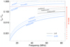 |
Fig. 10 fpe/fce values computed as in Fig. 8 but in the frequency range of NenuFAR. |
| In the text | |
|
Fig. A.1 Example of determination of the overall drift rate of sub-burst trains on 3 December 2021. (a) Five seconds of catalogued sub-bursts reproduced from Fig. 8c of Paper I. (b) Result of parametric linear de-dispersion and spectral integration of (a), as a function of slope (left scale) or drift rate (right scale). The dashed horizontal line about -500 MHz/s indicates the drift rate for which most of the burst clusters of (a) align. (c) Standard deviation of each line of (b) (actually exponential of values of (b) are used to enhance the contrast). The dashed vertical line indicates the peak value, obtained at −514 MHz/s. (d) Distribution of overall drift rates computed in 20 s × 30 MHz intervals between 1000 and 1150 MHz. For each of the 5 frequency intervals, the diamond indicates the average overall drift rate and the ‘+’ the 10 % and 90% quantiles of their distribution. The solid line is the linear fit of the average values, and the dashed lines those of the quantiles. The lower values about -1000 MHz/s are ‘saturated’ by the time resolution of the original dynamic spectrum (a), which prevents us from distinguishing clearly between drift rates steeper than -1000 MHz/s; we thus limited our parametric de-dispersion to that value. |
| In the text | |
|
Fig. B.1 Refractive Index, N, as a function of the frequency f (with ω = 2πf ) for a low-density plasma (i.e., fce > fpe, required for the ECM to occur). The red areas corresponds to the + branch of the Appleton-Hartree expression, while the blue area correspond to the - branch. The oblique propagation dispersion curves for different θ are shown as thin coloured lines (with δθ = 5°), while dispersion curves for parallel propagation (θ = 0°) are shown as thick black lines, and those for perpendicular propagation (θ = 90°) as thick black dashed lines. The frequencies of the L-mode cutoff fL, plasma cutoff fpe , cyclotron resonance fce , upper hybrid resonance fUH and R-mode cutoff fR , are indicated on the x-axis. In this example, fce/ fpe = 0.3. In reality, it is lower than that, but it has been enlarged here for the sake of readability. |
| In the text | |
|
Fig. B.2 Electron distribution functions able to amplify radio waves. (a) In a shell-type distribution, the ∇υ⊥ positive gradient of the distribution function is located along the inner edge of the distribution (red arrows). The ECM resonance circle leading to amplification is tangent to it and centred at υ‖0 = 0. (b) In a loss-cone distribution, the loss-cone is a region depleted in electrons, lost by collision with the atmosphere. This region is located below the dashed line, defined by the pitch angle α. The largest positive gradient ∇υ⊥ of the distribution function (red arrow) is along the edge of the loss-cone, at some resonance velocity υr. The ECM resonance circle leading to maximum amplification is tangent to this gradient, and is centred on υ‖0 = υr / cosα. The figure is reproduced from Hess et al. (2008). |
| In the text | |
|
Fig. C.1 Representative examples of simulated emission envelopes with ExPRES. R-X mode is emitted from the northern (a,c,e) or southern (b,d,f) hemisphere, by loss-cone-driven ECM with characteristic energy 10 keV (a,b), 30 keV (c,d), and 100 keV (e,f). Five dipolar magnetic shells (L=2, 5, 10, 20, 40) are simulated in each case, with active radio sources along all field lines at the corresponding magnetic shell (actually at every degree of longitude; small t–f gaps due to this discretisation have been interpolated). An Earth-based observer detects RH (black) or LH (red) polarised emission depending on the hemisphere of origin and emission mode. On all panels, bursts were detected by FAST in the green-shaded areas, while the green contours refer to uGMRT detections. |
| In the text | |
|
Fig. C.2 (continued) for loss-cone-driven ECM with characteristic energy 200 keV (g,h), and for shell-driven ECM (i,j). |
| In the text | |
Current usage metrics show cumulative count of Article Views (full-text article views including HTML views, PDF and ePub downloads, according to the available data) and Abstracts Views on Vision4Press platform.
Data correspond to usage on the plateform after 2015. The current usage metrics is available 48-96 hours after online publication and is updated daily on week days.
Initial download of the metrics may take a while.