| Issue |
A&A
Volume 695, March 2025
|
|
|---|---|---|
| Article Number | A35 | |
| Number of page(s) | 18 | |
| Section | Cosmology (including clusters of galaxies) | |
| DOI | https://doi.org/10.1051/0004-6361/202347761 | |
| Published online | 03 March 2025 | |
Homology reveals significant anisotropy in the cosmic microwave background
1
Univ Lyon, ENS de Lyon, Univ Lyon1, CNRS, Centre de Recherche Astrophysique de Lyon UMR5574, F–69007 Lyon, France
2
School of Artificial Intelligence, Bennett University, Plot no. 8 -12, Greater Noida, UP, India
3
Ashoka University, National Capital Region P.O., Plot no. 2, Rajiv Gandhi Education City, Rai, Sonipat, Haryana, India
⋆ Corresponding author; This email address is being protected from spambots. You need JavaScript enabled to view it.
, This email address is being protected from spambots. You need JavaScript enabled to view it.
Received:
18
August
2023
Accepted:
19
December
2024
Abstract
We test the tenet of statistical isotropy of the standard cosmological model via a homology analysis of the cosmic microwave background (CMB) temperature maps in galactic coordinates. The map pixels were normalized by subtracting the mean and rescaling by standard deviation, both of which were computed from the relevant unmasked pixels. Examining small sectors of the normalized maps, we find that the results exhibit a dependence on whether we compute the mean and variance locally from the non-masked patch, or from the full masked sky. Assigning local mean and variance for normalization, we find the maximum discrepancy between the data and model in the northern hemisphere, at more than 3.5 standard deviations (s.d.) for the PR4 dataset at degree scale. For the PR3 dataset, the C-R and SMICA maps display a higher significance than the PR4 dataset at ∼4 and 4.1 s.d., respectively; however, the NILC and SEVEM maps present a lower significance at ∼3.4 s.d. The discrepancy is most prominent at scales of roughly a degree, which coincides with the physical scale of the horizon at the epoch of the CMB. The southern hemisphere exhibits a high degree of consistency between the data and the model for both the PR4 and PR3 datasets. Assigning the mean and variance of the full masked sky decreases the significance for the northern hemisphere; in particular, the tails. However, the tails in the southern hemisphere are strongly discrepant at more than 4 standard deviations at approximately 5 degrees. The p values obtained from the χ2-statistic show commensurate significance in both experiments. Examining the quadrants of the sphere, we find the northwest quadrant of the Galactic frame to be the major source of the discrepancy. Prima facie, the results indicate a breakdown of statistical isotropy in the CMB maps; however, more work is needed to ascertain the source of the anomaly. Regardless, these map characteristics may have serious consequences for downstream computations and parameter estimation, and the related problems of Hubble and σ8 tension.
Key words: methods: data analysis / methods: numerical / methods: statistical / cosmic background radiation / cosmology: observations / early Universe
© The Authors 2025
 Open Access article, published by EDP Sciences, under the terms of the Creative Commons Attribution License (https://creativecommons.org/licenses/by/4.0), which permits unrestricted use, distribution, and reproduction in any medium, provided the original work is properly cited.
This article is published in open access under the Subscribe to Open model. This email address is being protected from spambots. You need JavaScript enabled to view it. to support open access publication.
1. Introduction
The standard Lambda cold dark matter (ΛCDM) paradigm of cosmology encapsulates and arises from the cosmological principle (CP), which posits that, on large enough scales, the Universe is isotropic and homogeneous (Milne 1936; Peebles & Yu 1970; Peebles 1980; Bardeen et al. 1986; Davis et al. 1985; Hamilton et al. 1986; Weinberg et al. 1987; White et al. 1993; Liddle & Lyth 2000; Harrison 2000; Saini et al. 2000; Durrer 2015; Jones 2017). Though supported by strong mathematical, philosophical, and historical foundations, the veracity of the fundamental tenets of CP has not yet been comprehensively and conclusively established, motivating theoretical and observational tests (Ellis & Baldwin 1984; Secrest et al. 2021; Oayda & Lewis 2023; Dam et al. 2023; Ragavendra et al. 2025). The recent focus of cosmology toward data gathering and analysis presents us with an unprecedented opportunity to test the postulates of the CP, and the ensuing standard model of cosmology. The data gathered are from both the early and late epochs in the evolutionary timeline of the Universe, and consistently present evidence for tensions and anomalies, including the discrepancy in the inference of the Hubble parameter and σ8 parameter between the data from the early and late Universe (Planck Collaboration XIII 2016; Planck Collaboration VI 2020; Burns et al. 2018; Freedman et al. 2019; Riess et al. 2021; Balkenhol et al. 2021; Rameez & Sarkar 2021; Abdalla et al. 2022; Sarkar 2022; Perivolaropoulos & Skara 2022; Aluri et al. 2023).
Cosmic microwave background (CMB) radiation is one of the more important probes of the properties of the early Universe. Emitted in the epoch of recombination, when the Universe was merely 380,000 years old, the fluctuation characteristics of the CMB trace the fluctuation characteristics of the matter distribution and represent an invaluable source of information on the properties of the early Universe (Sciama 1967; Silk 1968; Bond & Efstathiou 1984, 1987; Smoot et al. 1992; Seljak & Zaldarriaga 1999; de Bernardis et al. 2000; Bouchet & Gispert 1999; Bouchet et al. 2001; Jaffe et al. 2001; Bennett et al. 2003; Spergel et al. 2003, 2007; Planck Collaboration I 2014; Durrer 2015; Planck Collaboration XIII 2016a; Jones 2017; Planck Collaboration V 2020). They offer the largest and oldest canvas on which to test the postulates of CP. Therefore, studying the CMB fluctuations is essential for understanding the properties of the stochastic matter field in the early Universe. The two components of the CMB radiation – temperature and polarization – present independent probes into the properties of the primordial fluctuations (Seljak & Zaldarriaga 1997; Zaldarriaga & Seljak 1997; Durrer 1999; de Bernardis et al. 2000).
The general consensus is that the stochastic fluctuation field of the CMB is an instance of an isotropic and homogeneous Gaussian random field (Harrison 1970; Guth & Tye 1980; Adler 1981; Starobinsky 1982; Guth & Pi 1982; Bardeen et al. 1986; Bouchet 2004; Komatsu 2010, see also Buchert et al. (2017), and references therein for more recent investigations of Gaussianity). However, the investigation of CMB data has revealed multiple anomalous features since the launch of the Cosmic Background Explorer (COBE) satellite (Mather et al. 1991; Smoot et al. 1991; Wright et al. 1992). Due to its low resolution of approximately 7 degrees, the analysis of COBE data first revealed the truly large-scale anomalous lack of correlation in the CMB at 60 degrees and more (Hinshaw et al. 1996). The COBE team also pointed out the peculiarity of a very low quadrupole moment in the CMB data (Mather et al. 1991; Smoot et al. 1992). Subsequently, the analysis of data from the Wilkinson Microwave Anisotropy Probe (WMAP) (Bennett et al. 2003; Spergel et al. 2007) satellite, with a higher resolution, revealed a number of other anomalies at smaller scales that have persisted in the CMB measurements by the latest Planck satellite (Tegmark et al. 2003; Eriksen et al. 2004a; Park 2004; Planck Collaboration I 2014; Planck Collaboration XVI 2016; Planck Collaboration VII 2020). These anomalies, which have been detected in both the real and the harmonic space, seem to be at odds with the postulates of the standard cosmological model, and perhaps with the more fundamental CP itself.
Representative examples of anomalies in the harmonic space consist of the hemispherical power asymmetry (HPA) (Eriksen et al. 2004b; Hansen et al. 2004, 2009; Paci et al. 2010; Planck Collaboration XXIII 2014) or the cosmic hemispherical asymmetry (CHA) (Mukherjee & Souradeep 2016), the alignment of low multipoles (Tegmark et al. 2003; Copi et al. 2004, 2015; Schwarz et al. 2004, 2016), as well as the parity anomaly (Land & Magueijo 2005; Finelli et al. 2012; Planck Collaboration XXIII 2014). In particular, the power spectrum has been studied at large scales, for ℓ = 2, …, 40 (Eriksen et al. 2004b; Mukherjee & Souradeep 2016), which has later been extended to smaller scales, ℓ ∼ 600 (Hansen et al. 2009; Paci et al. 2010; Planck Collaboration XXIII 2014), and the analysis presents the evidence for HPA or CHA at all scales. Important to note is that the assumption of cosmological isotropy is challenged in other datasets as well (Bouchet et al. 2001; Colin et al. 2019; Secrest et al. 2021, 2022; Oayda & Lewis 2023; Dam et al. 2023). In particular, the analysis of galaxy survey datasets also points to a hemispherical asymmetry, as the northern and the southern galactic hemispheres appear to have different topo-geometrical characteristics (Kerscher et al. 1997, 1998, 2001; Appleby et al. 2022).
The anomalies in the real space have consisted of the discovery of the cold spot (Cruz et al. 2005), the anomalous low variance (Monteserín et al. 2008; Cruz et al. 2011), and the unusual behavior of descriptors emerging from topo-geometrical considerations that involve integral-geometric Minkowski functionals (MFs) (Adler 1981; Schmalzing & Buchert 1997; Sahni et al. 1998; Pranav et al. 2019a). It is interesting to note that while the purely geometric MFs such as the n-dimensional volume generally show consistency with the model, while the purely topological measures such as the genus and the Euler characteristic (Gott et al. 1986, 1989; Hamilton et al. 1986; Weinberg et al. 1987) hint at deviations from the standard model simulations. Analysis of the CMB maps using MFs was first performed on WMAP data (Schmalzing & Gorski 1998; Park 2004; Eriksen et al. 2004a) and later extended to Planck data (Planck Collaboration XXIII 2014; Planck Collaboration XVI 2016; Planck Collaboration VII 2020; Pranav et al. 2019b; Pranav 2021a, 2022). While Park (2004) performed their analysis on small sub-degree scales, Eriksen et al. (2004a) performed a multi-scale analysis spanning a range of sub- and super-degree scales. In both cases, there is reported asymmetry between the CMB hemispheres. The small-scale analysis in Park (2004) reports anomalous behavior to the tune of 2σ, while (Eriksen et al. 2004a) report a more than 3σ deviation in the genus statistic at scales of approximately 5 degrees for negative thresholds. In this context, it is important to note that the purely geometric entities of the MFs, such as the area, contour length, and skeleton length, have consistently shown a congruence between the data and the model (Planck Collaboration XVI 2016; Buchert et al. 2017), while the purely topological entities, such as the genus and the Euler characteristic, have consistently shown deviations between the data and the model (Eriksen et al. 2004a; Park 2004; Adler et al. 2017; Pranav 2021a, 2022).
Extending these studies, in this paper, we examine specific sectors of the CMB temperature maps with a view to test the tenet of statistical isotropy, via tools that have their basis in purely topological notions arising from homology (Munkres 1984; Edelsbrunner & Harer 2010; Pranav 2015; Pranav et al. 2017). Homology, together with its hierarchical extension, persistent homology (Edelsbrunner et al. 2002; Edelsbrunner & Harer 2010; Pranav 2015, 2021b, 2021c; Pranav et al. 2017, 2019a), forms the basis of the recently emerging field of topological data analysis (TDA) (Carlsson 2009; Wasserman 2018; Porter et al. 2023). Using these methodologies, which form the basis for the developed computational pipeline tailored to examining the CMB datasets (Pranav 2022), the central contribution of this paper is the uncovering of a number of anomalous signatures, which point to different behavior of galactic hemispheres. It is worth noting that evidence for the discovered anomalies has been documented in the literature in the past.
The advent of TDA holds an important place in view of the recent surge in data acquisition in cosmology and astronomy, which demands increasingly more sophisticated tools to condense meaningful information from these large and growing datasets. In view of these observations, the tools and methodologies presented here particularly stand out as promising candidates to reveal novel features in the big cosmological datasets, including the completed, ongoing, and upcoming CMB observations, as is evidenced in this paper, as well as galaxy surveys. Even though a recent development, TDA has already featured strongly in a wide range of astrophysical research, from studies on the large-scale structure of the Universe (van de Weygaert et al. 2011a, 2011b; Sousbie 2011; Shivashankar et al. 2016; Xu et al. 2019; Cisewski-Kehe et al. 2018, 2022; Codis et al. 2018; Feldbrugge et al. 2019; Biagetti et al. 2021; Kono et al. 2020; Wilding et al. 2021; Heydenreich et al. 2022; Elbers & van de Weygaert 2019; Ouellette et al. 2023) to studies on the stochastic properties of astrophysical and cosmological fields in general (Park et al. 2013; Adler et al. 2017; Makarenko et al. 2018; Pranav et al. 2019a; Heydenreich et al. 2022; Pranav 2021c), including the CMB fluctuation field (Adler et al. 2017; Pranav et al. 2019b; Pranav 2021a, 2022).
Section 2 presents a brief background on the topological concepts. Section 3 presents the data and methods, while Section 4 presents the main results. We discuss the results and conclude in Section 5.
2. Topological background
The methods employed in this paper emerge from algebraic and computational topology, at the level of homology (Munkres 1984; Edelsbrunner & Harer 2010) and persistent homology (Edelsbrunner et al. 2002; Edelsbrunner & Harer 2010). In this section, we describe the concepts that are essential for understanding the results presented in this paper in an intuitive fashion, referring the reader to Pranav et al. (2017) and Edelsbrunner & Harer (2010) for a more technical presentation.
These methodologies are complementary in nature to the integral-geometric Minkowski functionals (Mecke et al. 1994; Schmalzing & Buchert 1997; Schmalzing & Gorski 1998; Eriksen et al. 2004a; Matsubara 2010; Ducout et al. 2013; Buchert et al. 2017; Appleby et al. 2018; Chingangbam et al. 2017; Telschow et al. 2023), and together they represent a comprehensive topo-geometrical characterization of fields.
2.1. Homology
Homology provides for an exact and unambiguous way of differentiating between topological spaces by enumerating the holes of different dimensions they contain. As an illustration, we examine the different objects presented in Figure 1, which consist of a disk, an annulus, a sphere, and a torus. A disk is a single connected object with no additional topological structure. It is different from an annulus, because the annulus consists of a single connected ring that surrounds a hole. Similarly, the sphere is different from a disk and an annulus, as it consists of a single connected surface that encloses a void. Finally, the torus consists of a single connected surface that bounds a void inside the tube, and it also bounds the visible hole. In addition, the hole inside the tube also serves as a void. Formally, the connected objects, holes, and voids, and their generalizations in higher dimensions are associated with the homology group ℍp; p = 0, 1, 2, …, d, where d is the ambient dimension of the topological space. The holes are identified indirectly in homology, by detecting the cycles that bound them. In spatial 3D, intuitively, a 0-cycle is associated with a connected component1, and the gap between two connected components is the 0-dimensional hole that they bound. Connected components, or isolated objects, can also be thought of as a connected cluster of points, and so the 0-dimensional homology cycles are directly associated with clustering properties. A 1-cycle bounds a loop or a hole, and 2-cycle is a connected surface that bounds a 3D void. The rank of the homology group ℍp is the number of independent p-dimensional cycles or holes in a manifold, and is denoted by the p-th Betti number, βpBetti (1871), Edelsbrunner & Harer (2010), Pranav et al. (2017). The Betti numbers of the different topological objects illustrated in Figure 1 are enumerated in Table 1.
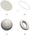 |
Fig. 1. Illustration of objects with different topologies, distinguished by the holes of different dimensions present in them. A disk (panel (a)) is characterized as a single connected object, while a ring (panel (b)) is characterized as a single connected object that forms the boundary of a hole. A sphere (panel (c)) is different from both a disk and a ring, as it is a single connected surface bounding the 3D cavity in the interior, while a torus (panel (d)) is characterized by a surface in the shape of a hollow tube that surrounds a visible hole, as well as the hole in the interior of the tube body, which also doubles up as a cavity or void. |
We imported the concepts from homology to study the topology of the temperature fluctuations of the CMB, defined on 𝕊2. In order to do so, we studied the excursion sets of the sphere, defined by the temperature function. For a given temperature, ν, the excursion set, 𝔼(ν), is given by
 (1)
(1)
On 𝕊2, only the 0- and 1D homology groups are of interest. They are associated with isolated components and holes of the excursion sets of 𝕊2. Figure 2 presents the excursion sets of 𝕊2 at three different temperature thresholds. At high positive thresholds in panel (a), we notice that the excursion set is exclusively composed of isolated objects or components. In experimental settings where the measurement is performed at discrete locations, these isolated objects usually consist of a cluster of points connected to each other, and the number of such independent objects is associated with 0, and represented by the 0-th Betti number, β0. At low negative thresholds, we notice that the excursion set is composed of a single connected surface, indented by multiple punctures. These punctures are related to topological loops or holes associated with the first homology group, 1, and the number of independent such loops counted by the first Betti number, β1. At sufficiently low thresholds, the excursion set forms the complete sphere, which is a single connected object with no punctures. However, for the complete sphere, there is a cavity enclosed by a surface. This cavity is associated with the second homology group, 2, and denoted by the second Betti number, β2.
 |
Fig. 2. Excursion sets of the 2-sphere at various thresholds of the temperature function defined on it. For high positive thresholds, the excursion set is predominantly composed of isolated objects or components. For low negative thresholds, the excursion set is composed of a single connected component, with additional punctures or loops. For low enough thresholds, the excursion set completes to form the full 2-sphere, composed of a single connected component and a void in the interior. |
2.2. Masks and relative homology
As was mentioned before, the topological entities on consist of components and holes, for both the excursion sets and the mask. In the presence of the mask, we computed the homology of the excursion sets, relative to the mask, and it differs from absolute homology. We did not count a component of the excursion set completely or partially overlapping with the mask, as it may be continuously shrunk into the mask through deformation retraction (Edelsbrunner & Harer 2010; Pranav et al. 2019b). A hole of the excursion set partially covered by the mask was still counted as a hole, as its boundary completes in the mask. A component of the mask was counted as a hole of the excursion set, and a hole of the mask contributed toward a void of the excursion set, as in such a case the excursion set is an open disk with its boundary in the mask, and therefore is homologous to 𝕊2. A more technical description of relative homology can be found in Pranav et al. (2019b).
2.3. Morse theory and persistent homology
According to Morse theory (Milnor 1963; Edelsbrunner & Harer 2010; Pranav et al. 2017), the topology of excursion sets of a function, f, changes only when passing through a critical point of the function. A critical point, x, is the location where the gradient of the function vanishes: ∇f(x)=0. The critical points are further differentiated by their index, which is the number of negative eigenvalues of the Hessian, given by
 (2)
(2)
In 2D, an index-0 critical point is a minimum, an index-1 critical point is a saddle point, and an index-2 critical point is a maximum. In d dimensions, an index-k critical point either gives birth to a (d − k)-dimensional topological cycle or destroys a k-dimensional cycle. As an example, a saddle point in 2D that has an index of 1 can have one of the two effects: it either connects two separate objects, reducing the number of connected objects by 1, or it connects the boundary of an already connected object, forming a 1-dimensional cycle bounding a loop. Therefore, each of the topological cycles in the growing excursion set is associated with a pair of critical points that are responsible for its birth and death.
The infinite values of thresholds corresponding to the excursion sets of a function are reduced to a finite number by recognizing that a finite manifold has a countably finite number of critical points, and that the topology of the excursion sets remains a constant between two critical points. Arranging the finitely many excursion sets corresponding to the critical points in a monotonically decreasing sequence results in a nested sequence of excursion sets known as a filtration. This filtration of excursion sets is hierarchical in nature, whereby the excursion set at a higher threshold is related to the excursion sets at a lower thresholds through a series of inclusion maps, which allows for tracking of the birth and death of topological cycles through the traversal of excursion sets. Persistent homology exploits the hierarchical nature of the filtration and the inclusion maps to determine the birth and death thresholds of all the unique topological events that occur through the traversal of the excursion sets, in terms of the values of the critical points associated with these events. The information of persistent homology is represented through persistence diagrams or barcodes Edelsbrunner et al. (2002), Carlsson et al. (2005). We employ the former in this paper to represent the information of persistent homology. A persistence diagram is a scatter plot in 2, where each of the dots in the diagram is associated with a unique topological feature born and destroyed in the filtration of the given function. There is a p-dimensional persistence diagram for each ambient dimension of the function, where p = 0, 1, …, d. The Betti numbers for a particular threshold, ν, can be extracted from the persistence diagrams. These are precisely the topological cycles that are born at or before ν, and that die after ν, or the cycles active at the threshold, ν.
2.4. Illustration
Figure 3 presents an illustration of the persistence diagrams and Betti numbers. The top row of the figure presents the illustration of the field on 𝕊2, derived from the CMB temperature fluctuation field smoothed with a Gaussian kernel of a full width at half maximum (FWHM) = 20 deg. The temperature fluctuation at each pixel was normalized by subtracting the mean and rescaling by the standard deviation of all pixels. The two panels of the second row from the top present the 0- and 1-dimensional persistence diagram, from left to right. In the third row from the top, we present the Betti number curves, and in the bottom row we present the excursion sets corresponding to ν = 1 and –1. In the left column, we note the presence of five connected components, while in the right we notice a single connected component with five punctures. Correspondingly, in the third row we read from the graphs of Betti numbers, β0(ν = 1)=4, β1(ν = −1)=4. In other words, the zeroth and the first Betti numbers have values one less than the number of components and the punctures. In the case of components, the component born at the highest threshold maps to the full surface at the lowest threshold, which belongs to the essential homology of the manifold, and we did not consider this component in our computations. In the case of punctures, a sphere with a single puncture on the surface is homeomorphic to a disk. Only additional punctures generate holes corresponding to the first homology group, and so we counted the number of holes as one less than the total number of punctures on the surface of the sphere.
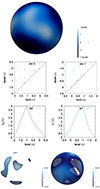 |
Fig. 3. Illustration of the computational aspects of homology and persistent homology. |
3. Data and methods
In this section, we briefly describe the data and methods employed for arriving at the results. All the computations were performed using TopoS2 (Pranav 2022), with the aid of HealPix (Górski et al. 2005) software for preprocessing. The computational pipeline, specifically tailored to the CMB data, but useful for the analysis of other scalar functions on 𝕊2, is a recent development, and a detailed account can be found in Pranav et al. (2019b) and Pranav (2022).
3.1. Data
The data that we investigated are the temperature maps from the latest two data releases by the Planck team – the penultimate Planck Data Release 3 (PR3) (Planck Collaboration IV 2020), and the fourth and final Planck Data Release 4 (PR4) (Planck Collaboration Int. LVII 2020). These data releases represent a natural evolution of the Planck data processing pipeline, whereby the final data release incorporates the best strategies for both the LFI and HFI instruments, commensurate with an overall reduction in noise and systematics (Planck Collaboration Int. LVII 2020). The PR3 and the PR4 datasets are accompanied by 600 and 300 simulations, respectively, which originate from the standard LCDM paradigm, which posits the CMB field to be an instance of an isotropic and homogeneous Gaussian random field. The PR3 dataset consists of observational maps obtained via four different component separation methods; namely, C-R, NILC, SEVEM, and SMICA (cf. Planck Collaboration I 2020). We analyzed all four maps in only one experiment, to assess the overall trend and congruence of results between the different component separation methods. This choice was dictated by significant computational overheads, especially for higher resolutions.
3.2. Computational methods
3.2.1. Masking and preprocessing
As the CMB component separation techniques are unreliable in the regions of strong galactic emissions, we masked these regions. We present our results in terms of the homology of the excursion sets relative to the mask, denoting the number of components relative to the mask for a given normalized threshold, ν, as b0(ν). A similar definition was adopted for the number of loops, b1(ν) (Pranav et al. 2019b; Pranav 2022). In a continuation of the experiments detailed in Pranav et al. (2019b) and Pranav (2021a,2022), in this paper we performed our investigations on the hemispheres and quadrants of the CMB sky, defined in galactic coordinates, as is presented in Table 2. When analyzing the northern hemisphere, the whole southern hemisphere and the relevant parts of northern hemisphere were masked, and vice versa. A similar masking procedure was adopted when examining the quadrants. Figure 4 presents a visualization of the temperature fluctuation field in the northern hemisphere, smoothed with a Gaussian beam profile of FWHM = 80′. Figure A.1 presents a visualization of the quadrants of the CMB sky in a Molleweide projection view.
Location of the sections of sky investigated in this paper, in galactic coordinates.
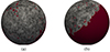 |
Fig. 4. Visualization of the CMB temperature fluctuation field in the northern hemisphere in two different views. The masked area covers the whole southern hemisphere and the relevant parts of the northern hemisphere, dictated by the PR3 temperature common mask. The visualization is based on the PR3 observed map, cleaned using the SMICA component separation pipeline, degraded at N = 128 and smoothed with a Gaussian kernel of FWHM = 80′. |
We performed a multi-scale analysis by smoothing the original maps given at FWHM = 5′ and N = 2048 to a range of scales defined by a Gaussian beam profile of FWHM = 10′,20′,40′,80′,160′,320′, and 640′. In order to facilitate faster computations, the maps were also degraded to N = 1024, 512, 256, 128, 64, 32, and 16 in the HealPix format (Górski et al. 2005). To execute these sets of operations, we adopted two different methods, which are briefly described below:
3.2.1.1. Method A.
In this procedure, we began by degrading the given maps at N = 2048 to the desired N. Subsequently, we extracted the spherical harmonic coefficient alm at the degraded resolution, and convolved it with the Gaussian beam at the desired FWHM value. Finally, we synthesized the maps from the Gaussian convolved alm at the final output resolution.
3.2.1.2. Method B.
In this procedure, we extracted the spherical harmonic coefficients at the input resolution and convolved them with the desired Gaussian beam profile at a given FWHM. Subsequently, we synthesized the maps directly at the given output resolution from the spherical harmonic coefficients. This is the process that is adopted as a standard, as for example by the Planck consortium in their analyses of the statistical properties of the CMB (Planck Collaboration VII 2020).
We find that the results from the two procedures vary in general, even though they exhibit similar characteristics broadly. In particular, method B yields stronger differences between the simulations and the observations. In the spirit of conservativeness, we present the results from method A in the main section of the paper. We also present a set of results from method B in the appendix for comparison.
The mask was subjected to an identical degrading and smoothing procedure. This resulted in a nonbinary mask that was re-binarized by setting all pixels above and equal to 0.9 to 1 and all pixels with smaller values to 0. The mask was applied to the simulations and observations, and they were transformed to zero-mean and unit-variance fields by subtracting the mean and rescaling by the standard deviation. Denoting δT(θ, ϕ) as the fluctuation field at (θ, ϕ) on 𝕊2, μδT as its mean, and σδT as the standard deviation, computed over the relevant pixels, we examined the properties of the normalized field:
 (3)
(3)
In all the experiments, we restricted ourselves to ν ∈ [0 : 3], while examining b0, and ν ∈ [ − 3 : 0] while examining b1, commensurate with the fact that components are the dominant topological entities at positive thresholds, while loops are dominant for the negative thresholds.
3.2.2. Topology computation
After the preprocessing steps explained in the previous section, performed with the aid of HealPix software (Górski et al. 2005), the data was subjected to the topology computation pipeline, which briefly involves tessellating the points on the sphere, computing the upper-star filtration of this tessellation, constructing the boundary matrix of the filtration, and reducing the boundary matrix to obtain the 0- and 1-dimensional persistence diagrams. The Betti numbers, relative to the mask, are condensed from the persistence diagrams. We describe these steps briefly below, referring the reader to Pranav et al. (2019b) and Pranav (2022) for details.
3.2.2.1. Triangulation.
We began by projecting the map pixels to 𝕊2, and constructing the triangulation, K, of the set of pixels in 3D. Taking the convex hull of the triangulation produces a triangulation on 𝕊2, which has V = 12N2 vertices, 3V − 6 edges, and 2V − 4 triangles, where N is the resolution parameter of the map in a HealPix format. This triangulation represents the CMB temperature function, f:𝕊2 → ℝ, where the temperature is stored at the vertices and all higher-dimensional simplices acquire a piecewise constant interpolation.
3.2.2.2. Upper star filtration.
To construct the upper star filtration, we ordered the simplices of the triangulation such that σ precedes τ if f(σ)> f(τ) or f(σ)=f(τ) and dim(σ)< dim(τ), where f(σ) is the minimum temperature value of the vertices of σ, and dim(σ) is the dimension of the simplex, σ. An ordering satisfying the above properties constitutes the upper-star filter of K and f, and the upper-star filtration consists of the prefixes of the filter, each representing an excursion set of f.
3.2.2.3. Boundary matrix construction, reduction, and persistence computation.
Given the upper star filtration, and given σ1, σ2, …, σn as the sorted simplices of the upper-star filtration, we defined the boundary matrix as ∂[1..n, 1..n] as ∂[i, j]=1, if σi is a face of σj and dim σi = dim σj − 1, and ∂[i, j]=0, otherwise. Thereafter, we reduced this ordered boundary matrix to a form commonly known as the lowest(j) form. In this matrix reduction method, a column of the matrix is considered reduced if all its elements in each row are uniformly zero throughout. If there are nonzero rows in a column, it is still considered reduced if the lowest row with nonzero entry has only zeros in the same row for all the columns to its left. The row and column indices increase from left to right and top to bottom in this convention. In the final reduced form, all the columns with nonzero entries have a unique row index for the lowest nonzero entry and the row and column indices of these entries determine the birth and death values associated with each unique topological feature in the persistence diagram. The birth and death coordinates of each dot in the persistence diagram correspond to the values on the simplices corresponding to the row and column indices of the lowest(j) (see also Pranav et al. 2017, 2019b).
3.2.2.4. Relative homology computation.
We determined the ranks of homology groups relative to the mask from the persistence diagrams by setting the vertices belonging to the mask at +∞, through the following set of equations:
 (4)
(4)
4. Results: Topological characteristics of subsets of 𝕊2
In this section, we present the results of the analysis of various sectors of the CMB sky, with a view to testing the statistical isotropy. We begin by presenting the results of examining the hemispheres, followed by an examination of the quadrants.
4.1. Hemispheres
For the hemispherical analysis, we present the results of two different experiments, which differ in the regions adopted to compute the mean and variance for normalizing the maps (cf. (3)). In the first experiment, we computed the mean and variance for each hemisphere locally from the unmasked pixels. In the second experiment, we computed the mean and variance from the unmasked pixels from the hemispheres. In all the experiments, we present our results in terms of the graphs of the Betti numbers relative to the mask. The graphs are normalized at each threshold to reflect the significance of deviation. At each threshold, we computed the mean, μbi, sim, and the standard deviation, σbi, sim, of the Betti numbers for i = 0, 1, corresponding to the components and the holes. Then, the significance of difference between the observation and simulations is given by
 (5)
(5)
which is the quantity depicted in the graphs.
4.1.1. Local normalization
For these experiments, the temperature at each pixel was mean-subtracted, and rescaled by the standard deviation, whereby these quantities were computed locally from the unmasked pixels in each hemisphere. The topological quantities were computed as a function of the normalized temperature threshold, ν ∈ [ − 3 : 3], in steps of 0.5. Figure 5 presents the graphs for the significance of difference between the simulations and the observations, for the number of components, b0, and the number of loops, b1, for the PR4 dataset. The red curve represents the observed sky, while the gray curves represent the individual simulations treated as observations. The top two rows present the graphs for b0 and b1 for the northern hemisphere, while the bottom two rows present the same for the southern hemisphere. Similar results for the PR3 dataset are presented in Figure B.3 in the appendix. In this case, we analyzed all four observational maps obtained from the different component separation pipeline.
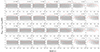 |
Fig. 5. Graphs of b0 and b1 for the temperature maps for the NPIPE dataset for the northern (top two rows) and southern (bottom two rows) hemispheres. The mean and variance were computed for each hemisphere locally from the unmasked pixels in that hemisphere. The graphs present the normalized differences, and each panel presents the graphs for a range of degradation and smoothing scales. The mask used is the PR3 temperature common mask. |
We notice a few important things in the graphs: first, that both the PR4 and PR3 datasets present largely identical results; and second, that the significance of deviation in the northern hemisphere is in general flared compared to the southern hemisphere. While the southern hemisphere significance is within the 2σ band in general, the northern hemisphere shows a significance of 2σ or more for most of the scales. The third important thing that we notice is the very significant deviation in the number of components between the observations and simulations at the threshold ν = 0.5, at FWHM = 80′,N = 128, which is approximately at the degree scale. The significance of the difference for the PR4 datasets stands at approximately 3.5σ. For the PR3 dataset, two of the maps, namely C-R and SMICA, exhibit a higher significance at approximately 4σ and 4.1σ, respectively, while the two other maps, namely NILC and SEVEM, display a 3.4σ deviation. Figure B.2 in the appendix presents the distribution of Betti numbers at this threshold, which can be approximated as a Gaussian; this justifies ascribing a σ significance to the differences. Figure A.2 presents the visualization of the structure of the temperature field at ν = 0.5 for the northern hemisphere. Clockwise from the top left, we present the field for the observed CMB map, as well as three randomly selected simulated samples that are presented in a different color scheme. We notice that the observed map exhibits smaller and more fragmented structures compared to the simulations. The largest connected structures in the observed and simulated maps are traced by connected edges, and it is evident that the simulations display larger connected structures compared to the observational map.
For the loops, the highest deviation recorded is at N = 64, FWHM = 160′ for the northern hemisphere. The PR4 dataset exhibits a 3.4σ deviation, while the PR3 dataset shows a 3.2σ deviation at this scale. At N = 128, FWHM = 80′, the PR4 dataset shows a maximum deviation of 3σ, while the PR3 dataset exhibits a 2.6σ deviation.
4.1.2. Global normalization
Figure 6 presents graphs similar to Figure 5 for the PR4 dataset, in which the maps are normalized by the mean and variance computed from unmasked pixels from the full sky. Similar results for the PR3 dataset are presented in Figure B.4. As in the case of local normalization, we notice an agreement in the features of the graphs between both datasets. However, we also note important differences between the observations and the simulations. For the northern hemisphere, the significance of difference is slightly suppressed in general, and there is an evident change in the behavior of the tail, where the observation is more consistent with the model. However, in this experiment there are significant differences between the observation and the model in the southern hemisphere. While the number of components, b0, is generally within the 2σ band, the number of loops exhibits strong differences between the data and model in the tail. This difference peaks at more than five standard deviations at scales of approximately 5 degrees and more. We note that the distribution of the Betti numbers is manifestly non-Gaussian at these scales and thresholds (cf. Pranav 2022).
 |
Fig. 6. Same as Figure 5; however, in this case, the mean and variance were computed from the full sky from the unmasked pixels. |
4.1.3. Significance of combined thresholds and resolutions
Table 3 presents the p values from the χ2 statistics for b0, b1, and ECrel for the PR4 dataset. ECrel is the alternating sum of the Betti numbers, and indicates the Euler characteristic of the excursion set relative to the mask. The p values for the PR3 dataset based on SMICA maps are presented in the Appendix in Table B.1. The first seven rows in the tables present the p values combining different thresholds for a given resolution, accounting for multiple testing at different thresholds. For both the datasets, the p values are consistent with the graphs, broadly indicating similar properties. For experiments in which the variance was computed separately for the hemispheres, there is a significant deviation between the data and the model approximately at a degree scale, at FWHM = 80′, for all the topological quantities. In addition, b0 exhibits differences for a range of scales at FWHM = 80′,160′, and 320′, with b1 also displaying mild differences. In contrast, the experiments with common variance exhibit a departure between the data and the model in the southern hemisphere at scales of 5 degrees and larger. The difference is most evident in the number of loops, which also affects the ECrel. However, we also note the deviant behavior of b0 at FWHM = 320′ in the northern hemisphere.
Two-tailed p values for relative homology obtained from the empirical Mahalanobis distance or χ2 test.
To account for multiple testing at various resolutions, the last entry in the tables presents the summary p values combining all the tested thresholds and resolutions. For the experiments in which the variance was computed separately for different hemispheres, the summary p values present significant evidence for nonrandom deviation for all the topological descriptors in the northern hemisphere. Similarly, for the experiments with a common variance computed from the full sky, the southern hemisphere indicates nonrandom discrepancy between the data and the model for all the topological descriptors, which is mild for b0 but significant for b1 and ECrel.
4.1.4. The effect of normalization
Normalization is an order-preserving transformation topologically. This ensures that there is a bijection between the original and the normalized maps, and specifically a correspondence in the dictionary of critical points as well as the order in which they appear in the filtration to form and destroy the topological cycles. This entails that, at the most, an erroneous estimation of mean and variance would induce an offset between the level sets of the compared maps, without affecting the deeper topological structure of the field. Combined with the fact that there are stark differences between the data and model irrespective of the recipe for normalization, this points to a difference in the topological structure of the observed field with respect to the simulations at a level deeper than normalization. Appendix B presents a short account of the properties of the distribution of the mean and variance for the full sky and the galactic hemispheres. At the level of mean, both the northern and the southern hemispheres are consistent between the data and model, which is reflected in the behavior of the mean in the full sky as well. In contrast, the variance of the northern hemisphere shows a stark deviation between the observation and simulations, while the variance in the southern hemisphere is consistent between the data and the model. This engenders a variance in the full sky case, which exhibits a mild deviation between the observation and simulations. Due to the evident discrepancy in variance, it is also prudent to treat both the hemispheres as arising from different models, and consequently treat the results from this experimental procedure in which the mean and variance were computed locally from the hemispheres as more meaningful. We note that the anomalous behavior of the variance found in our analysis is consistent with earlier reports of an anomalous variance (Planck Collaboration XXIII 2014), which was also found in the WMAP data (Monteserín et al. 2008; Cruz et al. 2011).
4.2. Quadrants of the sphere
Following the results of the previous section, in which we detected an anomalous behavior in the hemispheres, in this section we compare the behavior of the observations and simulations in the different quadrants of the sphere for the PR4 dataset, illustrated in Figure A.1, with a view to determine the zone of discrepancy more accurately. In these experiments, we computed the mean and the variance locally from the quadrants for map normalization. We restricted ourselves to the analysis of scales represented by FWHM = 20, 40, 80, 160, and 320. Our choice of scales was determined by the fact that at larger scales statistics on smaller sections of the sphere may not be reliable due to the low numbers involved, while the smaller scales have significant computational overheads.
Figure A.3 presents the graphs for the Betti numbers, while Table 4 presents the p values computed from the empirical χ2 test for the different quadrants, based on 600 simulations. Examining the graphs, the first quadrant stands out due to the maximum deviation for b1 at FWHM = 160′, with a significance of more than 3.8σ. The p values presented in Table 4 corroborate the fact that the northern hemisphere exhibits anomalous behavior with respect to the simulations, where the source of the discrepancy is clearly associated with the first quadrant. The summary p values combining all thresholds and resolutions indicate a strong nonrandom deviation between data and model in the first quadrant, which is strongest for b0. Interesting to note is that the deviations between the data and the model for the quadrants have shifted to a slightly higher resolution of FWHM = 160′, where b0 also exhibits the strongest deviations. In comparison, the quadrants of the southern hemisphere exhibit no difference with respect to the model, which is consistent with the observation that the southern Galactic hemisphere is congruent with the standard model, when the maps are normalized by local mean and variance.
Two-tailed p values for relative homology obtained from the empirical Mahalanobis distance or χ2 test.
4.3. Comparison with earlier results in literature
4.3.1. Local hemisphere variance.
In the experiments in which the variance was computed locally from the hemispheres, the most striking feature is the significant deviation at a degree scale in the northern hemisphere. We have noticed hints of this degree-scale deviation in the full sky analysis reported in Pranav (2022), in which we reported a 2.96σ deviation in the PR3 dataset at FWHM = 80′. The PR4 dataset at this scale exhibits a 2.2σ deviation. Due to a weak display of anomaly in the PR4 dataset, we rejected it in view of the larger scales exhibiting stronger anomalies statistically.
We find a similar phenomenon in the investigations on the WMAP data reported in the literature. Park (2004) and Eriksen et al. (2004a) pioneered the investigation of genus statistics of WMAP CMB data. While Park (2004) stuck to small sub-degree scales, Eriksen et al. (2004a) performed a multi-scale topo-geometrical investigation spanning a range from sub-degree small scales to super-degree large scales. Due to its multi-scale analysis, as well as the fact that it was performed on WMAP data and represents independent evidence, we find Eriksen et al. (2004a) an excellent source for comparison with our results. Figure 4 of Eriksen et al. (2004a) presents the Minkowski functional curves for the WMAP data smoothed at FWHM = 1.28 deg, where the genus in the positive threshold range deviates from the simulations at more than 2σ. This is more evident in the Figure 5 of Eriksen et al. (2004a), in which the MFs and the skeleton length are presented for a range of smoothing scales. We notice a discrepancy in the genus between observations and simulations at more than 2σ for positive thresholds for a range of scales, most prominently around 1.28 deg and 1.70 deg. The genus for the negative thresholds shows no anomaly at these scales. This also results in the suppression of the signal from the positive threshold anomaly in the χ2 statistic for the genus. Simultaneously, for the larger scales of approximately 5 degrees, the genus at negative thresholds deviates by more than 3σ, and therefore, like in our case in Pranav (2022), Eriksen et al. (2004a) also do not deem the degree scale deviation to be significant in view of the anomaly at larger scales. In the same paper, Figure 10 shows that the asymmetry parameter between negative and positive thresholds for the genus is weakly correlated. This is experimental evidence in support of the theoretical fact that the different Betti numbers, which dominate the genus at different thresholds, are independent, which further motivates the case for examining the Betti numbers separately, in addition to their linear combination, reflected in the genus. Our experiments further support this observation, as the Betti numbers of the hemispheres reveal a difference in their topological properties, which is the source of weak deviation observed in the full sky analysis for the Betti numbers, as well as the associated genus statistics, in both the Planck and WMAP data.
4.3.2. Global variance.
Assigning the global variance to the hemispheres gives rise to discrepant behavior between observations and simulations in the southern hemisphere, specifically for the loops at scales of roughly 5 degrees and larger. The observed discrepancy stands at approximately 5 standard deviations. We have also observed hints of this phenomenon in the full sky analysis, in which we report a difference of 3.9 standard deviation in the number of loops between the observations and simulations at this scale (Pranav 2022). The source of this deviation is linked to the strongly deviant behavior of loops in the southern hemisphere. Moreover, this phenomenon is also observed in the WMAP data, in which the genus at negative thresholds exhibits large deviations from the simulations at these scales (Eriksen et al. 2004a).
5. Discussions and conclusion
In this paper, we have presented a multi-scale analysis of the topological properties of the CMB temperature maps in small sectors of the sky, including hemispheres and quadrants, with the aim of investigating the veracity of the postulate of statistical isotropy. This is a continuation of the experiments performed in Pranav et al. (2019b) and Pranav (2021a,2022), in which we report on the full sky properties of the temperature fluctuation maps. We have employed tools emanating from homology and its hierarchical extension, persistent homology, which form the foundations of computational topology (Edelsbrunner et al. 2002; Edelsbrunner & Harer 2010; Pranav et al. 2017).
We have found various anomalous signatures in the topology of the temperature fluctuations in the normalized maps in small sections of the sky defined in the Galactic coordinates. In the case of hemispheres, the characteristics of the discovered anomalous signatures depend on the section of the sky adopted to compute the mean and variance for normalizing the maps. For experiments in which the hemispheres were assigned a local mean and variance for normalization, we find that the northern hemisphere shows significant deviations between the data and the model, most prominently at scales of roughly a degree, in which case the coincidence between the scale of the anomaly and the horizon at the epoch of CMB is worth noting. The anomalous signatures in this case are more prominent for topological components; however, the topological holes also present anomalous behavior. In contrast, the southern hemisphere displays a remarkable consistency with the standard model simulations. For the experiments in which the hemispheres were assigned a global mean and variance computed from the masked full sky, the southern hemisphere exhibits strongly anomalous behavior with respect to the standard model simulations at scales of roughly 5 degrees and more.
Noting that the variance of the northern hemisphere is starkly different, while the variance of the southern hemisphere is strongly consistent with the model, it may be prudent to treat the hemispheres as arising from different models at the level of normalization. Consequently, the results from the experiments in which the variance was computed locally from the hemispheres may be a more accurate reflection of reality than the experiments in which the hemispheres were assigned a global variance for normalization. In view of this, the degree-scale anomalies in the behavior of the topological components in the northern hemisphere may be a stronger and fairer indicator of the ground truth, compared to the larger-scale anomalies in the topological loops in the southern hemisphere that could be artifacts of data treatment. Taking hints from the experiments on the hemispheres, we further tested the quadrants of the sphere assigning local variance for normalization. In this case, we find that the first quadrant displays significantly anomalous behavior with respect to the simulations.
Despite possible offsets due to an erroneous estimation of mean and variance, considering the fact that normalization is an order-preserving transformation, and that the anomalies persist irrespective of the recipe adopted for normalization, this points to deeper differences in the stochastic structure of the observed and simulated CMB fields, at a level beyond normalization and offset effects. The fact that the deviations persist in the χ2 tests, which take into consideration all the thresholds and resolutions, is another compelling argument against the deviations being engendered by offset effects. However, to avoid and mitigate any such effects, in future research we shall present a comparison of topology directly in the space of persistence diagrams, which encode consolidated information about all level sets. Preliminary inroads in this direction have been been made in terms of modeling persistence diagrams directly, with an analysis of the Galactic hemispheres in Adler et al. (2017).
An agnostic interpretation of these data characteristics points to a departure from statistical isotropy in the CMB maps; however, further work is required to convincingly ascribe the source of the anomalies to a genuinely cosmological effect, a foreground effect (Bouchet & Gispert 1999), or merely systematic effects. Regarding noise and systematics, there is an important point to consider from first principles. The PR4 dataset purportedly has a lower level of systematics and noise compared to the PR3 dataset. If this is the ground truth, and if the anomalous signals that we have discovered are real, their significance should increase from PR3 to the PR4 datasets. We notice this trend for the NILC and SEVEM maps, but the opposite trend for C-R and SMICA maps, which makes any assessment about the origin of the signals inconclusive. It is also important to note that the slightly differing results for the different maps in PR3 indicate the sensitivity of our methodology to the details of the component separation pipeline, and can be considered as a framework for benchmarking.
In the context of foregrounds (Bouchet & Gispert 1999), the recently discovered foreground effect by Hansen et al. (2023) also deserves a specific mention. They find that there is an effect of deepening of the CMB temperature profile extending to a few degrees around nearby large spiral galaxies. They posit that this foreground effect may provide a possible common explanation for a number of anomalies of different kinds in the CMB. In the context of the topological anomalies, such an effect may generate spurious holes in addition to deepening their temperature profiles. However, we find it difficult to conclude that the aforementioned foreground can account for the novel anomalous signatures presented in this paper, for a few reasons. First, the evidence presented in this paper points to strongly anomalous signatures in the hot spot regions also, which cannot be explained by the deepening of temperature profiles, or the creation of spurious cold spots. Second, the fact that an anomalous number of cold spots appear in the southern hemisphere when assigning a global variance for normalization, and disappear when normalizing the hemispheres by local variance, points to the fact that the anomalous behavior of the cold spots in the southern hemisphere may in fact be misleading, and engendered as an artifact of data processing. The third compelling reason is that we find the deviations to be the most significant in the first quad in galactic coordinates, and the foreground map presented in Hansen et al. (2023) lacks significant foreground contamination in this region. Regardless of the finer details, a crucial point to note from the evidence presented in this paper is that the disagreement between the data and the model may engender spurious results for all subsequent downstream calculations, such as cosmological parameter estimation (Fosalba & Gaztañaga 2021; Yeung & Chu 2022), and may have consequences for the Hubble and σ8 tension through the related misestimation of cosmological parameters.
A topological component is different from the components of the measured sky signals in the context of observations, in which component separation refers to signal processing techniques that extract CMB and foreground from the total measured signals.
Acknowledgments
We thank the anonymous referee for the numerous incisive comments and suggestions that have improved the manuscript significantly. We are indebted to Herbert Edelsbrunner, Rien van de Weygaert, Armin Schwartzman, and Robert Adler for discussions and comments that have helped shape the draft. We are grateful to Hans Kristian Eriksen, Mohammed Rameez and Geraint F. Lewis for important comments on the draft. PP would also like to acknowledge the crucial interactions with Reijo Keskitalo and Julian Borill, their consistent help with questions, and incisive comments on the draft. PP is partially supported by the Simons-Ashoka fellowship (grant no: 993444). This work is part of a project that has received funding from the European Research Council (ERC) under the European Union’s Horizon 2020 research and innovation programme (grant agreement ERC advanced grant 740021 – ARTHUS, PI: TB). A part of this work was supported by the Physics of Living Matter Group at the University of Luxembourg, and by the Luxembourg National Research Fund’s ATTRACT Investigator Grant no. A17/MS/11572821/MBRACE, and CORE Grant no. C19/MS/13719464/TOPOFLUME. We gratefully acknowledge the support of PSMN (Pôle Scientifique de Modélisation Numérique) of the ENS de Lyon, and the Department of Energy’s National Energy Research Scientific Computing Center (NERSC) at Lawrence Berkeley National Laboratory, operated under Contract No. DE-AC02-05CH11231, for the use of computing resources.
References
- Abdalla, E., Abellán, G. F., Aboubrahim, A., et al. 2022, J. High Energy Astrophys., 34, 49 [NASA ADS] [CrossRef] [Google Scholar]
- Adler, R. 1981, The Geometry of Random Fields, Classics in applied mathematics (Society for Industrial and Applied Mathematics (SIAM, 3600 Market Street, Floor 6, Philadelphia, PA 19104)) [Google Scholar]
- Adler, R. J., Agami, S., & Pranav, P. 2017, PNAS, 114, 11878 [NASA ADS] [CrossRef] [Google Scholar]
- Aluri, P. K., Cea, P., Chingangbam, P., et al. 2023, CQG, 40, 094001 [NASA ADS] [CrossRef] [Google Scholar]
- Appleby, S., Chingangbam, P., Park, C., Yogendran, K. P., & Joby, P. K. 2018, ApJ, 863, 200 [NASA ADS] [CrossRef] [Google Scholar]
- Appleby, S., Park, C., Pranav, P., et al. 2022, ApJ, 928, 108 [CrossRef] [Google Scholar]
- Balkenhol, L., Dutcher, D., Ade, P., et al. 2021, Phys. Rev. D, 104, 083509 [NASA ADS] [CrossRef] [Google Scholar]
- Bardeen, J. M., Bond, J. R., Kaiser, N., & Szalay, A. S. 1986, ApJ, 304, 15 [Google Scholar]
- Bennett, C. L., Halpern, M., Hinshaw, G., et al. 2003, ApJS, 148, 1 [Google Scholar]
- Betti, E. 1871, Ann. Mat. Pura Appl., 2, 140 [Google Scholar]
- Biagetti, M., Cole, A., & Shiu, G. 2021, JCAP, 2021, 061 [CrossRef] [Google Scholar]
- Bond, J. R., & Efstathiou, G. 1984, ApJ, 285, L45 [NASA ADS] [CrossRef] [Google Scholar]
- Bond, J. R., & Efstathiou, G. 1987, MNRAS, 226, 655 [NASA ADS] [Google Scholar]
- Bouchet, F. R. 2004, arXiv e-prints [arXiv:astro-ph/0401108] [Google Scholar]
- Bouchet, F. R., & Gispert, R. 1999, New Astron., 4, 443 [NASA ADS] [CrossRef] [Google Scholar]
- Bouchet, F. R., Peter, P., Riazuelo, A., & Sakellariadou, M. 2001, Phys. Rev. D, 65, 021301 [NASA ADS] [CrossRef] [Google Scholar]
- Buchert, T., France, M. J., & Steiner, F. 2017, CQG, 34, 094002 [NASA ADS] [CrossRef] [Google Scholar]
- Burns, C. R., Parent, E., Phillips, M. M., et al. 2018, ApJ, 869, 56 [Google Scholar]
- Carlsson, G. 2009, Bull. Am. Math. Soc., 46, 255 [CrossRef] [Google Scholar]
- Carlsson, G., Zomorodian, A., Collins, A., & Guibas, L. J. 2005, Int. J. Shape Model., 11, 149 [CrossRef] [Google Scholar]
- Chingangbam, P., Yogendran, K. P., Joby, P. K., et al. 2017, JCAP, 12, 023 [CrossRef] [Google Scholar]
- Cisewski-Kehe, J., Wu, M., Fasy, B., et al. 2018, Am. Astron. Soc. Meet. Abstr., 231, 213.07 [NASA ADS] [Google Scholar]
- Cisewski-Kehe, J., Fasy, B. T., Hellwing, W., et al. 2022, Phys. Rev. D, 106, 023521 [NASA ADS] [CrossRef] [Google Scholar]
- Codis, S., Pogosyan, D., & Pichon, C. 2018, MNRAS, 479, 973 [Google Scholar]
- Colin, J., Mohayaee, R., Rameez, M., & Sarkar, S. 2019, A&A, 631, L13 [NASA ADS] [CrossRef] [EDP Sciences] [Google Scholar]
- Copi, C. J., Huterer, D., & Starkman, G. D. 2004, Phys. Rev. D, 70, 043515 [NASA ADS] [CrossRef] [Google Scholar]
- Copi, C., Huterer, D., Schwarz, D., & Starkman, G. 2015, MNRAS, 449, 3458 [NASA ADS] [CrossRef] [Google Scholar]
- Cruz, M., Martínez-González, E., Vielva, P., & Cayón, L. 2005, MNRAS, 356, 29 [CrossRef] [Google Scholar]
- Cruz, M., Vielva, P., Martínez-González, E., & Barreiro, R. B. 2011, MNRAS, 412, 2383 [CrossRef] [Google Scholar]
- Dam, L., Lewis, G. F., & Brewer, B. J. 2023, MNRAS, 525, 231 [NASA ADS] [CrossRef] [Google Scholar]
- Davis, M., Efstathiou, G., Frenk, C. S., & White, S. D. M. 1985, ApJ, 292, 371 [Google Scholar]
- de Bernardis, P., Ade, P. A. R., Bock, J. J., et al. 2000, Nature, 404, 955 [Google Scholar]
- Ducout, A., Bouchet, F. R., Colombi, S., Pogosyan, D., & Prunet, S. 2013, MNRAS, 429, 2104 [NASA ADS] [CrossRef] [Google Scholar]
- Durrer, R. 1999, New Astron. Rev., 43, 111 [CrossRef] [Google Scholar]
- Durrer, R. 2015, CQG, 32, 124007 [NASA ADS] [CrossRef] [Google Scholar]
- Edelsbrunner, H., & Harer, J. 2010, in Computational Topology: An Introduction, (American Mathematical Society), Applied mathematics [Google Scholar]
- Edelsbrunner, H., Letscher, J., & Zomorodian, A. 2002, Discrete Comput. Geom., 28, 511 [CrossRef] [Google Scholar]
- Elbers, W., & van de Weygaert, R. 2019, MNRAS, 486, 1523 [Google Scholar]
- Ellis, G. F. R., & Baldwin, J. E. 1984, MNRAS, 206, 377 [NASA ADS] [CrossRef] [Google Scholar]
- Eriksen, H. K., Novikov, D. I., Lilje, P. B., Banday, A. J., & Górski, K. M. 2004a, ApJ, 612, 64 [NASA ADS] [CrossRef] [Google Scholar]
- Eriksen, H. K., Hansen, F. K., Banday, A. J., Górski, K. M., & Lilje, P. B. 2004b, ApJ, 605, 14 [NASA ADS] [CrossRef] [Google Scholar]
- Feldbrugge, J., van Engelen, M., van de Weygaert, R., Pranav, P., & Vegter, G. 2019, JCAP, 2019, 052 [CrossRef] [Google Scholar]
- Finelli, F., Gruppuso, A., Paci, F., & Starobinsky, A. A. 2012, JCAP, 2012, 049 [Google Scholar]
- Fosalba, P., & Gaztañaga, E. 2021, MNRAS, 504, 5840 [Google Scholar]
- Freedman, W. L., Madore, B. F., Hatt, D., et al. 2019, ApJ, 882, 34 [Google Scholar]
- Górski, K. M., Hivon, E., Banday, A. J., et al. 2005, ApJ, 622, 759 [Google Scholar]
- Gott, J. R., III, Dickinson, M., & Melott, A. L. 1986, ApJ, 306, 341 [NASA ADS] [CrossRef] [Google Scholar]
- Gott, J. R., III, Miller, J., Thuan, T. X., et al. 1989, ApJ, 340, 625 [NASA ADS] [CrossRef] [Google Scholar]
- Guth, A. H., & Pi, S.-Y. 1982, PRL, 49, 1110 [NASA ADS] [CrossRef] [Google Scholar]
- Guth, A. H., & Tye, S.-H. H. 1980, PRL, 44, 631 [NASA ADS] [CrossRef] [Google Scholar]
- Hamilton, A. J. S., Gott, J. R., III, & Weinberg, D. 1986, ApJ, 309, 1 [Google Scholar]
- Hansen, F. K., Cabella, P., Marinucci, D., & Vittorio, N. 2004, ApJ, 607, L67 [NASA ADS] [CrossRef] [Google Scholar]
- Hansen, F. K., Banday, A. J., Górski, K. M., Eriksen, H. K., & Lilje, P. B. 2009, ApJ, 704, 1448 [NASA ADS] [CrossRef] [Google Scholar]
- Hansen, F. K., Boero, E. F., Luparello, H. E., & Garcia Lambas, D. 2023, A&A, 675, L7 [NASA ADS] [CrossRef] [EDP Sciences] [Google Scholar]
- Harrison, E. R. 1970, Phys. Rev. D, 1, 2726 [CrossRef] [Google Scholar]
- Harrison, E. 2000, Cosmology: The Science of the Universe (Cambridge University Press) [CrossRef] [Google Scholar]
- Heydenreich, S., Brück, B., Burger, P., et al. 2022, A&A, 667, A125 [NASA ADS] [CrossRef] [EDP Sciences] [Google Scholar]
- Hinshaw, G., Banday, A. J., Bennett, C. L., et al. 1996, ApJ, 464, L25 [NASA ADS] [CrossRef] [Google Scholar]
- Jaffe, A. H., Ade, P. A. R., Balbi, A., et al. 2001, PRL, 86, 3475 [NASA ADS] [CrossRef] [Google Scholar]
- Jones, B. J. T. 2017, Precision Cosmology: The First Half Million Years (Cambridge University Press) [CrossRef] [Google Scholar]
- Kerscher, M., Schmalzing, J., Buchert, T., & Wagner, H. 1997, in Research in Particle-Astrophysics, eds. R. Bender, T. Buchert, P. Schneider, & F. von Feilitzsch, 83 [Google Scholar]
- Kerscher, M., Schmalzing, J., Buchert, T., & Wagner, H. 1998, A&A, 333, 1 [NASA ADS] [Google Scholar]
- Kerscher, M., Mecke, K., Schmalzing, J., et al. 2001, A&A, 373, 1 [NASA ADS] [CrossRef] [EDP Sciences] [Google Scholar]
- Komatsu, E. 2010, CQG, 27, 124010 [NASA ADS] [CrossRef] [Google Scholar]
- Kono, K. T., Takeuchi, T. T., Cooray, S., Nishizawa, A. J., & Murakami, K. 2020, arXiv e-prints [arXiv:2006.02905] [Google Scholar]
- Land, K., & Magueijo, J. 2005, Phys. Rev. D, 72, 101302 [NASA ADS] [CrossRef] [Google Scholar]
- Liddle, A. R., & Lyth, D. H. 2000, Cosmological Inflation and Large-Scale Structure (Cambridge University Press), 414 [Google Scholar]
- Makarenko, I., Bushby, P., Fletcher, A., et al. 2018, J. Plasma Phys., 84, 047303 [CrossRef] [Google Scholar]
- Mather, J. C., Hauser, M. G., Bennett, C. L., et al. 1991, Adv. Space Res., 11, 181 [NASA ADS] [CrossRef] [Google Scholar]
- Matsubara, T. 2010, Phys. Rev. D, 81, 083505 [NASA ADS] [CrossRef] [Google Scholar]
- Mecke, K. R., Buchert, T., & Wagner, H. 1994, A&A, 288, 697 [NASA ADS] [Google Scholar]
- Milne, E. A. 1936, Philosophy, 11, 95 [CrossRef] [Google Scholar]
- Milnor, J. 1963, Morse Theory (Princeton: Princeton University Press) [Google Scholar]
- Monteserín, C., Barreiro, R. B., Vielva, P., et al. 2008, MNRAS, 387, 209 [Google Scholar]
- Mukherjee, S., & Souradeep, T. 2016, PRL, 116, 221301 [NASA ADS] [CrossRef] [Google Scholar]
- Munkres, J. 1984, in Elements of Algebraic Topology, (Perseus Books), Advanced book classics [Google Scholar]
- Oayda, O. T., & Lewis, G. F. 2023, MNRAS, 523, 667 [NASA ADS] [CrossRef] [Google Scholar]
- Ouellette, A., Holder, G., & Kerman, E. 2023, MNRAS, 523, 5738 [NASA ADS] [CrossRef] [Google Scholar]
- Paci, F., Gruppuso, A., Finelli, F., et al. 2010, MNRAS, 407, 399 [NASA ADS] [CrossRef] [Google Scholar]
- Park, C.-G. 2004, MNRAS, 349, 313 [NASA ADS] [CrossRef] [Google Scholar]
- Park, C., Pranav, P., Chingangbam, P., et al. 2013, JKAS, 46, 125 [NASA ADS] [Google Scholar]
- Peebles, P. 1980, in The Large-scale Structure of the Universe, (Princeton University Press), Princeton series in physics [Google Scholar]
- Peebles, P. J. E., & Yu, J. T. 1970, ApJ, 162, 815 [NASA ADS] [CrossRef] [Google Scholar]
- Perivolaropoulos, L., & Skara, F. 2022, New Astron. Rev., 95, 101659 [CrossRef] [Google Scholar]
- Planck Collaboration I. 2014, A&A, 571, A1 [NASA ADS] [CrossRef] [EDP Sciences] [Google Scholar]
- Planck Collaboration XXIII. 2014, A&A, 571, A23 [NASA ADS] [CrossRef] [EDP Sciences] [Google Scholar]
- Planck Collaboration XIII. 2016, A&A, 594, A13 [NASA ADS] [CrossRef] [EDP Sciences] [Google Scholar]
- Planck Collaboration XVI. 2016, A&A, 594, A16 [NASA ADS] [CrossRef] [EDP Sciences] [Google Scholar]
- Planck Collaboration I. 2020, A&A, 641, A1 [NASA ADS] [CrossRef] [EDP Sciences] [Google Scholar]
- Planck Collaboration IV. 2020, A&A, 641, A4 [NASA ADS] [CrossRef] [EDP Sciences] [Google Scholar]
- Planck Collaboration V. 2020, A&A, 641, A5 [NASA ADS] [CrossRef] [EDP Sciences] [Google Scholar]
- Planck Collaboration VI. 2020, A&A, 641, A6 [NASA ADS] [CrossRef] [EDP Sciences] [Google Scholar]
- Planck Collaboration VII. 2020, A&A, 641, A7 [NASA ADS] [CrossRef] [EDP Sciences] [Google Scholar]
- Planck Collaboration Int. LVII. 2020, A&A, 643, A42 [NASA ADS] [CrossRef] [EDP Sciences] [Google Scholar]
- Porter, M. A., Feng, M., & Katifori, E. 2023, Phys. Today, 76, 36 [CrossRef] [Google Scholar]
- Pranav, P. 2015, Ph.D. Thesis, University of Groningen, The Netherlands [Google Scholar]
- Pranav, P. 2021a, arXiv e-prints [arXiv:2101.02237] [Google Scholar]
- Pranav, P. 2021b, IEEE SPM, 38, 130 [NASA ADS] [Google Scholar]
- Pranav, P. 2021c, arXiv e-prints [arXiv:2109.08721] [Google Scholar]
- Pranav, P. 2022, A&A, 659, A115 [NASA ADS] [CrossRef] [EDP Sciences] [Google Scholar]
- Pranav, P., Edelsbrunner, H., van de Weygaert, R., et al. 2017, MNRAS, 465, 4281 [Google Scholar]
- Pranav, P., van de Weygaert, R., Vegter, G., et al. 2019a, MNRAS, 485, 4167 [Google Scholar]
- Pranav, P., Adler, R. J., Buchert, T., et al. 2019b, A&A, 627, A163 [EDP Sciences] [Google Scholar]
- Ragavendra, H. V., Mukherjee, D., & Sethi, S. K. 2025, PRD, 111, 023541 [NASA ADS] [CrossRef] [Google Scholar]
- Rameez, M., & Sarkar, S. 2021, CQG, 38, 154005 [CrossRef] [Google Scholar]
- Riess, A. G., Casertano, S., Yuan, W., et al. 2021, ApJ, 908, L6 [NASA ADS] [CrossRef] [Google Scholar]
- Sahni, V., Sathyprakash, B., & Shandarin, S. 1998, ApJ, 507, L109 [NASA ADS] [CrossRef] [Google Scholar]
- Saini, T. D., Raychaudhury, S., Sahni, V., & Starobinsky, A. A. 2000, PRL, 85, 1162 [NASA ADS] [CrossRef] [Google Scholar]
- Sarkar, S. 2022, Inf.: Int. Rev. Sci., 6, 4 [Google Scholar]
- Schmalzing, J., & Buchert, T. 1997, ApJ, 482, L1 [NASA ADS] [CrossRef] [Google Scholar]
- Schmalzing, J., & Gorski, K. M. 1998, MNRAS, 297, 355 [CrossRef] [Google Scholar]
- Schwarz, D. J., Starkman, G. D., Huterer, D., & Copi, C. J. 2004, PRL, 93, 221301 [NASA ADS] [CrossRef] [Google Scholar]
- Schwarz, D. J., Copi, C. J., Huterer, D., & Starkman, G. D. 2016, CQG, 33, 184001 [NASA ADS] [CrossRef] [Google Scholar]
- Sciama, D. W. 1967, PRL, 18, 1065 [NASA ADS] [CrossRef] [Google Scholar]
- Secrest, N. J., von Hausegger, S., Rameez, M., et al. 2021, ApJ, 908, L51 [Google Scholar]
- Secrest, N. J., von Hausegger, S., Rameez, M., Mohayaee, R., & Sarkar, S. 2022, ApJ, 937, L31 [NASA ADS] [CrossRef] [Google Scholar]
- Seljak, U., & Zaldarriaga, M. 1997, PRL, 78, 2054 [NASA ADS] [CrossRef] [Google Scholar]
- Seljak, U., & Zaldarriaga, M. 1999, PRL, 82, 2636 [NASA ADS] [CrossRef] [Google Scholar]
- Shivashankar, N., Pranav, P., Natarajan, V., et al. 2016, IEEE Trans. Vis. Comput. Graph., 22, 1745 [CrossRef] [Google Scholar]
- Silk, J. 1968, ApJ, 151, 459 [NASA ADS] [CrossRef] [Google Scholar]
- Smoot, G. F., Bennett, C. L., Kogut, A., et al. 1991, Adv. Space Res., 11, 193 [NASA ADS] [CrossRef] [Google Scholar]
- Smoot, G. F., Bennett, C. L., Kogut, A., et al. 1992, ApJ, 396, L1 [Google Scholar]
- Sousbie, T. 2011, MNRAS, 414, 350 [NASA ADS] [CrossRef] [Google Scholar]
- Spergel, D. N., Verde, L., Peiris, H. V., et al. 2003, ApJS, 148, 175 [Google Scholar]
- Spergel, D. N., Bean, R., Doré, O., et al. 2007, ApJS, 170, 377 [NASA ADS] [CrossRef] [Google Scholar]
- Starobinsky, A. A. 1982, Phys. Lett. B, 117, 175 [Google Scholar]
- Tegmark, M., de Oliveira-Costa, A., & Hamilton, A. J. 2003, PRD, 68, 123523 [NASA ADS] [CrossRef] [Google Scholar]
- Telschow, F. J. E., Cheng, D., Pranav, P., & Schwartzman, A. 2023, Ann. Stat., 51, 2272 [CrossRef] [Google Scholar]
- van de Weygaert, R., Vegter, G., Edelsbrunner, H., et al. 2011a, Trans. Comput. Sci., XIV, 60 [NASA ADS] [CrossRef] [Google Scholar]
- van de Weygaert, R., Pranav, P., Jones, B. J. T., et al. 2011b, arXiv e-prints [arXiv:1110.5528] [Google Scholar]
- Wasserman, L. 2018, Annu. Rev. Stat. Appl., 5, 501 [CrossRef] [Google Scholar]
- Weinberg, D. H., Gott, J. R., III, & Melott, A. L. 1987, ApJ, 321, 2 [NASA ADS] [CrossRef] [Google Scholar]
- White, S. D. M., Efstathiou, G., & Frenk, C. S. 1993, MNRAS, 262, 1023 [NASA ADS] [CrossRef] [Google Scholar]
- Wilding, G., Nevenzeel, K., van de Weygaert, R., et al. 2021, MNRAS, 507, 2968 [NASA ADS] [CrossRef] [Google Scholar]
- Wright, E. L., Meyer, S. S., Bennett, C. L., et al. 1992, ApJ, 396, L13 [NASA ADS] [CrossRef] [Google Scholar]
- Xu, X., Cisewski-Kehe, J., Green, S., & Nagai, D. 2019, Astron. Comput., 27, 34 [NASA ADS] [CrossRef] [Google Scholar]
- Yeung, S., & Chu, M.-C. 2022, PRL, 105, 083009 [Google Scholar]
- Zaldarriaga, M., & Seljak, U. 1997, Phys. Rev. D, 55, 1830 [Google Scholar]
Appendix A: Additional figures
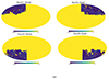 |
Fig. A.1. An illustration of the analyzed map surface in the different quadrants of the sphere. The first, second, third and fourth quadrants are presented from left to right, and this convention is followed for quoting the results. |
 |
Fig. A.2. A visualization of the structure of the superlevel set of the temperature field at the threshold ν = 0.5 for the northern hemisphere. This is the threshold at which we detect a statistically significant deviation between the observation and simulations in the number of isolated components. The top-left panel presents the visualization of the observed CMB map from PR3 data release. The rest of the panels present the visualization for the randomly selected simulation sample from the FFP10 simulation set, numbering 42, and its two higher multiples 84 and 126. All the maps are smoothed with a Gaussian beam profile of FWHM = 80′. At the level of visual examination, we find that the observational map is composed of larger number of smaller structures compared to the simulations, which display the evidence of larger structures. The largest connected structure in the observational and simulated maps are traced by green connected segments for reference. It is evident that the simulations are characterized by larger such structures compared to the observational map. |
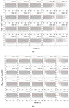 |
Fig. A.3. Graphs of b0 and b1 for the different quadrants of the sphere for a range of smoothing scales with Gaussian FWHM = 20′,40′,80′,160′,320′. Panel (a) presents the graphs for b0 while panel (b) presents the graphs for b1. The values for the different quadrants are presented from top to bottom, while the scale increases from left to right. |
Appendix B: Distribution characteristics of mean, variance and Betti numbers
In the results presented in the previous sections, we have noticed features in the topological characteristics that exhibit weak to strong dependence on the recipe for computing mean and variance for normalizing the maps. Specifically, computing the mean and variance locally from the hemispheres points to a difference between the data and model in the northern hemisphere, as opposed to the southern hemisphere that shows remarkable consistency with the model. In contrast, computing the variance from the full sky results in a deviation between the data and model for both the hemispheres for some scales.
As the anomalies presented in the previous sections exhibit a dependence on the recipe for computing mean and variance, we examine the histograms of mean and variance of the hemispheres and the full sky at N = 512 in Figure B.1. From the figure, we notice the variance of the observation in the northern hemisphere to be less than the variance from all the 600 simulated maps, while the southern sky is consistent with the simulations. As a result, the full sky exhibits mildly anomalous characteristics with respect to the simulations. When examining the mean, it is evident that both the northern and the southern skies are consistent with the simulations. It has also been noted in the literature that at all scales the northern hemisphere exhibits anomalous variance with respect to the simulations, in contrast with the southern hemisphere, which exhibits no deviation Planck Collaboration XXIII (2014). It may therefore be prudent to treat the hemispheres as arising from different models, when computing the mean and variance for normalization.
Figure B.2 presents the histogram of b0 from the simulations for this threshold and resolution, with the observed value indicated by a red vertical line. It is evident from the histogram that the distribution maybe approximated by a Gaussian distribution.
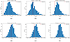 |
Fig. B.1. Histogram of variance for the north, south and full sky, with the appropriate regions masked. The histograms are computed for the map at N = 512. |
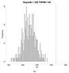 |
Fig. B.2. Histogram of b0 values at ν = 0.5 for the PR3 dataset at FWHM = 80′. The distribution from the simulations indicates a tendency toward a symmetric Gaussian distribution. |
B.1. PR3 dataset
In this section, we present the graphs and table of p values for the PR3 dataset. Figure B.3 presents the graphs of the Betti numbers for the maps that are normalized with respect to local mean and variance, while Figure B.4 presents the graphs for normalization where the mean and the variance as computed from the masked full sky. The graphs display consistent characteristics with that of the PR4 dataset presented in the main body of the paper, albeit with higher significance of difference between the data and the model. Table B.1 presents the p values computed from the χ2-statistic. The top seven rows present the χ2-statistic computed from the combined level sets for a given resolution, while the bottom row presents the same for the combination of all thresholds at all resolutions. Commensurate with the graphs, the p values for the PR3 dataset presents higher significance of difference between the data and the model.
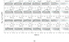 |
Fig. B.3. Graphs for local normalization. Graphs of b0 and b1 for the temperature maps for the PR3 dataset for the northern (top two rows) and the southern hemisphere (bottom two rows)The variance is computed for each hemisphere separately from the unmasked pixels in that hemisphere. The graphs present the normalized differences, and each panel presents the graphs for a range of degradation and smoothing scales. The mask used is the PR3 temperature common mask. |
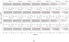 |
Fig. B.4. Graphs for global normalization. Graphs of b0 and b1 for the temperature maps for the PR3 dataset for the northern (top two rows) and the southern hemispheres (bottom two rows). The graphs present the normalized differences, and each panel presents the graphs for a range of degradation and smoothing scales. The variance is computed from the full sky from the unmasked pixels. The mask used is the PR3 temperature common mask. |
Significance of difference for the hemispheres in PR3 dataset.
Appendix C: Results from method B
In this Section, we presents thew graphs of Betti numbers and the p-value tables method B, where we extract the alm coefficients from the maps at the original resolution, convolve them with the given Gaussian beam profile, and subsequently synthesize the maps directly at the output resolution form the alm’s.
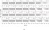 |
Fig. C.1. Graphs of b0 and b1 for the temperature maps for the PR4 dataset computed from method B. The top two rows present the graphs for the northern hemisphere, and the bottom two rows for the southern hemisphere. The graphs present the normalized differences, and each panel presents the graphs for a range of degradation and smoothing scales. The variance is computed from the hemispheres locally from the unmasked pixels. The mask used is the PR3 temperature common mask. |
Significance of difference for the PR4 dataset for method B.
All Tables
Location of the sections of sky investigated in this paper, in galactic coordinates.
Two-tailed p values for relative homology obtained from the empirical Mahalanobis distance or χ2 test.
Two-tailed p values for relative homology obtained from the empirical Mahalanobis distance or χ2 test.
All Figures
|
Fig. 1. Illustration of objects with different topologies, distinguished by the holes of different dimensions present in them. A disk (panel (a)) is characterized as a single connected object, while a ring (panel (b)) is characterized as a single connected object that forms the boundary of a hole. A sphere (panel (c)) is different from both a disk and a ring, as it is a single connected surface bounding the 3D cavity in the interior, while a torus (panel (d)) is characterized by a surface in the shape of a hollow tube that surrounds a visible hole, as well as the hole in the interior of the tube body, which also doubles up as a cavity or void. |
| In the text | |
|
Fig. 2. Excursion sets of the 2-sphere at various thresholds of the temperature function defined on it. For high positive thresholds, the excursion set is predominantly composed of isolated objects or components. For low negative thresholds, the excursion set is composed of a single connected component, with additional punctures or loops. For low enough thresholds, the excursion set completes to form the full 2-sphere, composed of a single connected component and a void in the interior. |
| In the text | |
|
Fig. 3. Illustration of the computational aspects of homology and persistent homology. |
| In the text | |
|
Fig. 4. Visualization of the CMB temperature fluctuation field in the northern hemisphere in two different views. The masked area covers the whole southern hemisphere and the relevant parts of the northern hemisphere, dictated by the PR3 temperature common mask. The visualization is based on the PR3 observed map, cleaned using the SMICA component separation pipeline, degraded at N = 128 and smoothed with a Gaussian kernel of FWHM = 80′. |
| In the text | |
|
Fig. 5. Graphs of b0 and b1 for the temperature maps for the NPIPE dataset for the northern (top two rows) and southern (bottom two rows) hemispheres. The mean and variance were computed for each hemisphere locally from the unmasked pixels in that hemisphere. The graphs present the normalized differences, and each panel presents the graphs for a range of degradation and smoothing scales. The mask used is the PR3 temperature common mask. |
| In the text | |
|
Fig. 6. Same as Figure 5; however, in this case, the mean and variance were computed from the full sky from the unmasked pixels. |
| In the text | |
|
Fig. A.1. An illustration of the analyzed map surface in the different quadrants of the sphere. The first, second, third and fourth quadrants are presented from left to right, and this convention is followed for quoting the results. |
| In the text | |
|
Fig. A.2. A visualization of the structure of the superlevel set of the temperature field at the threshold ν = 0.5 for the northern hemisphere. This is the threshold at which we detect a statistically significant deviation between the observation and simulations in the number of isolated components. The top-left panel presents the visualization of the observed CMB map from PR3 data release. The rest of the panels present the visualization for the randomly selected simulation sample from the FFP10 simulation set, numbering 42, and its two higher multiples 84 and 126. All the maps are smoothed with a Gaussian beam profile of FWHM = 80′. At the level of visual examination, we find that the observational map is composed of larger number of smaller structures compared to the simulations, which display the evidence of larger structures. The largest connected structure in the observational and simulated maps are traced by green connected segments for reference. It is evident that the simulations are characterized by larger such structures compared to the observational map. |
| In the text | |
|
Fig. A.3. Graphs of b0 and b1 for the different quadrants of the sphere for a range of smoothing scales with Gaussian FWHM = 20′,40′,80′,160′,320′. Panel (a) presents the graphs for b0 while panel (b) presents the graphs for b1. The values for the different quadrants are presented from top to bottom, while the scale increases from left to right. |
| In the text | |
|
Fig. B.1. Histogram of variance for the north, south and full sky, with the appropriate regions masked. The histograms are computed for the map at N = 512. |
| In the text | |
|
Fig. B.2. Histogram of b0 values at ν = 0.5 for the PR3 dataset at FWHM = 80′. The distribution from the simulations indicates a tendency toward a symmetric Gaussian distribution. |
| In the text | |
|
Fig. B.3. Graphs for local normalization. Graphs of b0 and b1 for the temperature maps for the PR3 dataset for the northern (top two rows) and the southern hemisphere (bottom two rows)The variance is computed for each hemisphere separately from the unmasked pixels in that hemisphere. The graphs present the normalized differences, and each panel presents the graphs for a range of degradation and smoothing scales. The mask used is the PR3 temperature common mask. |
| In the text | |
|
Fig. B.4. Graphs for global normalization. Graphs of b0 and b1 for the temperature maps for the PR3 dataset for the northern (top two rows) and the southern hemispheres (bottom two rows). The graphs present the normalized differences, and each panel presents the graphs for a range of degradation and smoothing scales. The variance is computed from the full sky from the unmasked pixels. The mask used is the PR3 temperature common mask. |
| In the text | |
|
Fig. C.1. Graphs of b0 and b1 for the temperature maps for the PR4 dataset computed from method B. The top two rows present the graphs for the northern hemisphere, and the bottom two rows for the southern hemisphere. The graphs present the normalized differences, and each panel presents the graphs for a range of degradation and smoothing scales. The variance is computed from the hemispheres locally from the unmasked pixels. The mask used is the PR3 temperature common mask. |
| In the text | |
Current usage metrics show cumulative count of Article Views (full-text article views including HTML views, PDF and ePub downloads, according to the available data) and Abstracts Views on Vision4Press platform.
Data correspond to usage on the plateform after 2015. The current usage metrics is available 48-96 hours after online publication and is updated daily on week days.
Initial download of the metrics may take a while.