| Issue |
A&A
Volume 694, February 2025
|
|
|---|---|---|
| Article Number | A154 | |
| Number of page(s) | 11 | |
| Section | Stellar atmospheres | |
| DOI | https://doi.org/10.1051/0004-6361/202452879 | |
| Published online | 11 February 2025 | |
Temperature and density profiles in the corona of main-sequence stars induced by stochastic heating in the chromosphere
1
Dipartimento di Fisica e Astronomia, Università di Firenze,
via G. Sansone 1,
50019
Sesto Fiorentino,
FI,
Italy
2
LESIA, Observatoire de Paris, Université PSL, CNRS, Sorbonne Université, Université Paris-Cité,
5 place Jules Janssen,
92195
Meudon,
France
3
INAF – Osservatorio Astrofisico di Arcetri,
Largo E. Fermi 5,
50125
Firenze,
Italy
4
INFN, Sezione di Firenze,
via G. Sansone 1,
50019
Sesto Fiorentino,
FI,
Italy
★ Corresponding author; This email address is being protected from spambots. You need JavaScript enabled to view it.
Received:
4
November
2024
Accepted:
20
January
2025
Abstract
All but the most massive main-sequence stars are expected to have a rarefied and hot (million-Kelvin) corona like the Sun. How such a hot corona is formed and supported has not been completely understood yet, even in the case of the Sun. Recently, a new model of a confined plasma atmosphere has been introduced and applied to the solar case, showing that rapid, intense, intermittent and short-lived heating events in the high chromosphere can drive the coronal plasma into a stationary state with temperature and density profiles similar to those observed in the solar atmosphere. In this paper we apply the model to main-sequence stars, showing that it predicts the presence of a solar-like hot and rarefied corona for all such stars, regardless of their mass. However, the model is not applicable as such to the most massive main-sequence stars, because the latter lack the convective layer generating the magnetic field loop structures supporting a stationary corona, whose existence is assumed by the model. We also discuss the role of stellar mass in determining the shape of the temperature and density profiles.
Key words: plasmas / methods: analytical / Sun: atmosphere / Sun: corona / stars: atmospheres / stars: coronae
© The Authors 2025
 Open Access article, published by EDP Sciences, under the terms of the Creative Commons Attribution License (https://creativecommons.org/licenses/by/4.0), which permits unrestricted use, distribution, and reproduction in any medium, provided the original work is properly cited.
This article is published in open access under the Subscribe to Open model. This email address is being protected from spambots. You need JavaScript enabled to view it. to support open access publication.
1 Introduction
The density of the Sun steadily decreases from its centre to the outermost layer of its atmosphere, the corona, which is extremely rarefied, being more than one million times less dense than the surface (photosphere). On the contrary, the temperature of the Sun decreases only up to the first layers of the atmosphere above the photosphere, and then starts to increase reaching millions of Kelvins in the corona, which is therefore more than two hundred times hotter than the photosphere (Golub & Pasachoff 2009). This temperature increase while density decreases, often referred to as ‘temperature inversion’, happens quite abruptly. Most of both the temperature jump and the density drop occur in the so-called ‘transition region’, a thin (only hundreds of kilometres wide) layer separating the lowest layer of the Sun’s atmosphere, the chromosphere, from the corona. Most of the plasma in the corona is organised in loops, following the magnetic field lines which exit the photosphere and then re-enter it, and emits radiation in the X band (Aschwanden 2005). An X-ray emission has been detected in many other main-sequence stars, regardless of the spectral type (Pallavicini 1989; Gudel 2004; Ness et al. 2004). Since all the main-sequence stars with mass M < 1.5 M⊙ have a convective region below the photosphere where a Sun-like magnetic field originates (see e.g. Maoz 2007), the X-ray emission is thought to be of coronal origin and all the late-type (from late spectral type A onwards) main-sequence stars are thought to have a corona analogous to the solar one, organised in loop structures and with a temperature around 106 K. A strong hint at the presence of a corona made up of Sun-like magnetic structures is that the relation between the X-ray luminosity and the magnetic field strength follows the same power law in both the Sun’s active regions (Fisher et al. 1998) and the atmospheres of less massive main-sequence stars (Pevtsov et al. 2003). The case of the most massive main-sequence stars (that is, O, B and up to early-A spectral type) is different because these stars lack a convective region below the photosphere and therefore should not have a solar-like magnetic field able to support a stationary corona: the X-ray emission from these stars is not attributed to a coronal activity but rather to strong winds and shocks (Pallavicini 1989; Gudel 2004).
Despite decades of investigation, the mechanism producing the million-Kelvin corona of the Sun (and of the other stars as well) is largely not yet understood. This open problem is referred to as the coronal heating problem (Klimchuk 2006; Parnell & De Moortel 2012). Most efforts have been conducted along the lines of finding suitable mechanisms able to transport energy from the lower layers to coronal heights, or to release energy stored in the magnetic field, and to efficiently dissipate such an energy in the corona (Parker 1972; Dmitruk & Gomez 1997; Gudiksen & Nordlund 2005; Rappazzo et al. 2008; Rappazzo & Parker 2013; Wilmot-Smith 2015; Heyvaerts & Priest 1983; Ionson 1978; Howson et al. 2020; Pontieu et al. 2011; Shoda & Takasao 2021; Shoda et al. 2024; Airapetian et al. 2021). Scudder (1992a,b) proposed a different approach, observing that collisions in the very dilute coronal plasma are rare and therefore the corona might be out of thermal equilibrium. Thus, if the velocity distribution functions of the particles at the base of the corona, that is, in the upper chromosphere, are non-Maxwellian, and in particular have suprathermal tails (that is, the probability of finding fast particles is larger than in a Maxwellian), then faster particles are able to climb higher in the gravitational potential well. As a result, the temperature increases with height while the density decreases. Such a mechanism was dubbed ‘velocity filtration’ or ‘gravitational filtering’. At variance with the above-mentioned approaches, Scudder’s model does not involve any local deposition of heat in the corona and is able to reproduce coronal temperatures and densities; however, it predicts a smooth change of the latter quantities, without a rapid increase of temperature, and its basic assumption of non-Maxwellian distribution functions for particles in the collisional chromosphere is difficult to justify.
In the highly collisional environment of the Sun’s chromosphere, any deviation from thermal distributions is expected to be extremely short-lived. Therefore, particles’ distribution functions in the chromosphere are expected to be thermal. This notwithstanding, the chromosphere is a very dynamic environment and its temperature is expected to fluctuate in space and time (Molnar et al. 2019). Starting from this observation, Barbieri et al. (2024a,b) recently reconsidered Scudder’s pioneering intuition, replacing the (hardly justifiable) assumption of non-thermal distributions in the high chromosphere with the hypothesis of a fluctuating temperature in an otherwise fully collisional and thermal chromosphere. Barbieri et al. (2024a,b) showed that rapid, intense, intermittent and short-lived temperature increments in the high chromosphere are able to drive the above plasma atmosphere towards a stationary configuration with an inverted temperature-density profile; in particular, the resulting temperature profile exhibits a steep rise of the temperature for not-so-large heights above the surface, similar to – albeit thicker than – the observed transition region, followed by a much less steep increase of the temperature for larger heights, very similar to the Sun’s hot corona (Yang et al. 2009). According to this model, the mechanism producing temperature inversion in the solar atmosphere is velocity filtration as in Scudder’s model, but there is no need to postulate distribution functions with suprathermal tails in the chromosphere: the latter are self-consistently produced by the gravitational filtering itself, and originate in the superposition of different thermal distributions in the chromosphere. Temperature fluctuations are modelled by a stochastic process, and essentially any probability distribution such that more intense fluctuations are less frequent than less intense ones works. Remarkably, no fine-tuning of the parameters is required to produce temperature inversion, the only requirement being that the temperature fluctuations are fast enough to prevent the system from relaxing towards a thermal configuration (for the Sun, this means that fluctuations must occur on a subsecond timescale, which is unresolved in current solar observations). The average intensity of the fluctuations, however, must be sufficiently large as to produce coronal temperatures. Indeed, short-lived, intense, and small-scale brightenings are routinely observed on the Sun (Dere et al. 1989; Teriaca et al. 2004; Peter et al. 2014; Tiwari et al. 2019; Berghmans et al. 2021). The so-called campfires recently observed in extreme UV images have temperatures of the order of 106 K, while explosive events appearing in Hα line widths have smaller temperatures, about 2 × 10⁵ K, but are ten times more frequent (Teriaca et al. 2004). This trend is consistent with the distribution of rapid temperature increments assumed in the model. Moreover, based on recent extreme UV solar observations, Raouafi et al. (2023) have shown that small-scale magnetic reconnection events at the base of the solar corona can produce a flow of matter that propagates up into the corona with the correct energy budget to heat the plasma environments up to million degrees.
Since a Sun-like hot corona is expected to be present in low-mass main-sequence stars (that is, stars with M < 1.5 M⊙), and the velocity filtration mechanism is very general and does not require any Sun-specific feature, in the present paper we apply the model proposed by Barbieri et al. (2024a,b) to main- sequence stars. More specifically, we want to answer the following questions: Does the model predict an inverted temperaturedensity profile with a rapid increase of temperature and a hot corona for all main-sequence stars? How are these profiles affected by the mass of the star?
The paper is structured as follows. In Sect. 2, we briefly review the plasma atmosphere model proposed by Barbieri et al. (2024a,b): more specifically, in Sect. 2.1 we describe the model and define its parameters, and in Sect. 2.2 we discuss the mechanism according to which the model produces a Sunlike temperature profile and a hot corona, defining a quantity that discriminates the range of parameters in which a solar-like corona does actually form from those in which it does not, and which will be useful in the following. In Sect. 3 we apply the theoretical framework to main-sequence stars and we present and discuss the results, focusing on the case of low-mass stars (M < 1.5 M⊙; the case of higher-mass stars is considered in Appendix A). Finally, in Sect. 4 we summarise our findings, we discuss the physical limits of our modelling and hint at some possible follow-ups of the present work.
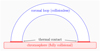 |
Fig. 1 Schematics of the loop model. The coronal plasma in the loop is treated as collisionless and in thermal contact with a fully collisional chromosphere (modelled as a thermostat). |
2 The model
2.1 Model description
Here we briefly summarise the model of the plasma atmosphere introduced by Barbieri et al. (2024a,b). A coronal loop in the atmosphere of a star is modelled as a semicircular tube of length 2L made up of a two-component (electrons and protons), collisionless electrostatic plasma subjected to an external force field consisting of a constant gravity plus an electric field ensuring charge neutrality and proportional to 𝑔(me + mp)/2, where me and mp are the masses of the electrons and of the ions, respectively (Pannekoek 1922; Rosseland 1924; Belmont et al. 2013), and 𝑔 = GM/R2 is the surface gravity with M and R the mass and radius of the star, respectively. Particles are allowed to move only along the loop. This structure is assumed to be in ideal thermal contact with a thermostat that mimics the fully collisional chromosphere. A scheme of the model is shown in Figure 1. If the temperature Tb of the thermostat (that is, of the chromosphere) is constant, the coronal loop is in thermal equilibrium at the same temperature of the thermostat. However, as mentioned in the Introduction, the chromosphere is a very dynamic environment; therefore, we assume that its temperature fluctuates due to heating events of amplitude ΔT and duration τ, separated by waiting times tw during which the temperature of the thermostat switches back to Tb. A sketch of the time series of the temperature of the thermostat is depicted in Figure 2. We keep τ fixed and we draw ΔT and tw from probability distributions. If the following conditions are fulfilled,
 (1)
(1)
where tr is the relaxation time in the corona and ⟨·⟩η is the average over a given probability distribution η, then the coronal plasma never relaxes to thermal equilibrium: it rather reaches a stationary state always exhibiting inverted temperature and density profiles. The relaxation time tr can be estimated as the minimum between the thermal crossing time tT and the free-fall crossing time t𝑔 of the electrons, that is,
 (2)
(2)
where
 (3)
(3)
In Eq. (3) above, ⟨T⟩γ is the average of T over a given probability distribution γ of temperature increments and kB is the Boltzmann constant.
Since the coronal plasma dynamics is treated as collisionless, the time evolution of the distribution functions of both species obeys Vlasov equations (see e.g. Nicholson 1983). By time averaging the Vlasov dynamics and the fluctuating thermostat over a timespan long enough to encompass many temperature increments, it is possible to analytically calculate the full phase-space distribution functions in the steady state (for details see Barbieri et al. 2024b). The resulting expressions for the single-particle phase space distribution functions fe and fp of electrons and ions, respectively, are
![Mathematical equation: ${f_\alpha }(x,\v ) = {{\cal N}_\alpha }\left[ {(1 - A){{{e^{ - {{{H_\alpha }(x,\v )} \over {{k_B}{T_b}}}}}} \over {{T_b}}} + A\,\int_{{T_b}}^{ + \infty } d T\,\gamma (T){{{e^{ - {{{H_\alpha }(\alpha ,\v )} \over {{k_B}T}}}}} \over T}} \right],$](/articles/aa/full_html/2025/02/aa52879-24/aa52879-24-eq4.png) (4)
(4)
where a = e or p, the constant A is given by
 (5)
(5)
and Hα is the single particle energy of the species α, that is,
 (6)
(6)
where v is the particle velocity and
 (7)
(7)
is the height upon the surface at a given position corresponding to a curvilinear abscissa x ∈ [−L, L] along the loop.
The constants 𝒩α are normalisation constants, so that the distribution functions fα are normalised to 1.
The interpretation of Eq. (4) is as follows: the distribution functions in the stationary state are given by a thermal distribution at temperature Tb (the reference temperature of the thermostat) plus a non-thermal contribution resulting from the average of thermal distributions at a temperature T > Tb over the probability distribution γ(T) of the temperature increments. The weight of the non-thermal contribution is proportional to A, which is the fraction of time the thermostat is not at temperature T = Tb, that is, the fraction of time in which the chromosphere is actually heated. The thermal population dominates at small heights ɀ and is suppressed by the gravitational term in Hα as ɀ increases; conversely, the non-thermal contribution becomes increasingly relevant at larger ɀ due to velocity filtration, as faster particles can climb higher in the potential well and appear as suprathermal tails in the distribution functions.
To perform the calculations, we choose the distributions of the temperature increments, γ, to be an exponential distribution,
 (8)
(8)
where 〈ΔT〉 = (T − Tb)γ is the mean value of the temperature increments.
This is the simplest choice guaranteeing that large temperature increments are less likely than small ones, as suggested, for instance, by the fact that the so-called ‘campfires’ recently observed in extreme UV solar imaging have temperatures of about 106 K, while explosive events appearing in Hα line widths have smaller temperatures, about 2 × 10⁵ K, but are ten times more frequent (Teriaca et al. 2004). However, Barbieri et al. (2024b) have shown that the precise choice of the distribution γ(T) is not very relevant, since the stationary state always exhibits temperature inversion, regardless of the choice of the distribution of the temperature increments. The choice of the distribution η(tw) of the waiting times between temperature increments is even less relevant, since it enters Eq. (4) only through the constant A defined in Eq. (5), which in turn depends only on ⟨tw⟩η, that is, on the average value of tw.
Once the functional form of the probability distribution γ is fixed, the distribution functions, Eq. (4), from which all the physical quantities in the stationary state can be derived only depend on three parameters: the surface gravity 𝑔, the average of the temperature increments 〈ΔT〉 and the fraction of time A the thermostat spends at a temperature larger than the reference one. Choosing the following set of units,
 (9)
(9)
which imply that the unit of energy is E0 = kBTb, where Tb is the unit of temperature, the two parameters 𝑔 and 〈ΔT〉 can be replaced by their dimensionless counterparts  and
and  . Therefore, the three dimensionless parameters upon which the model depends are the constant A given by Eq. (5), the strength
  of the external field in units of thermal energy,
 (10)
(10)
and the average amplitude of temperature increments  measured in units of the reference temperature Tb of the thermostat,
 (11)
(11)
The larger the parameter  defined in Eq. (10) above, the stronger the stratification of the atmosphere is. Therefore we shall refer to
  as the stratification parameter. If A ≠ 0, the temperature T(ɀ) at any height ɀ within the loop will be strictly larger than the reference thermostat temperature Tb. Requiring that the temperature at the base of the loop, T(ɀ = 0), is fixed and close to the average observed value at the base of the corona, one gets an implicit relation between A and
  , so that the latter two parameters arr independent and the free parameters of the model are reduced to two, which ce no longean be chosen as
  and
and  . In the following, we shall assume, as in Barbieri et al. (2024a,b), that the temperature at the base of the corona is 10% larger than Tb, that is, T(ɀ = 0) = 1.1 Tb.
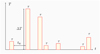 |
Fig. 2 Sketch of the time series of the temperature of the thermostat (chromosphere). During the time intervals of duration τ the temperature increases by an amount ΔT and during the waiting times tw it returns to the typical chromospheric value Tb. |
2.2 Sun-like atmosphere
In Sect. 3 and in Appendix A, we shall apply the above-described model to main-sequence stars, asking whether and under which conditions it predicts the presence of a Sun-like corona in such stars. To do so, we shall first examine the temperature and density profiles in two examples and clarify what does it mean, in the framework of this model, to exhibit a Sun-like corona. Then we shall introduce an ad-hoc quantity, X, that depends on the parameters of the model,  and
and  , and whose value is used to discriminate between the presence or absence of a Sunlike corona without having to inspect temperature and density profiles.
The temperature T and the number density n can be computed at any point of the loop from the stationary distribution functions (4) according to the standard kinetic definitions (see e.g. Nicholson 1983), and turn out to be equal for both species. We say that the model predicts a Sun-like corona when the variation of temperature T and the number density n as a function of the height ɀ within the loop has the following representative properties, as shown in Fig. 3. First, there is a steep rise in T and a steep fall in n at small heights, ɀ, analogous to what happens in the Sun’s transition region. Second, at the top of the region where the temperature rapidly increases the density and temperature have already coronal values, that is, T ≈ 102 Tb and n ≈ 10−3 n0. where n0 = n(ɀ = 0) is the density at the base of the loop. Third, at larger heights, both the temperature increase and the density decrease are much gentler.
As discussed by Barbieri et al. (2024a,b), these profiles are very similar to those of the atmosphere of the Sun, but for the fact that the interval of heights where the temperature steeply increases is thicker than the observed transition region. The profiles plotted in Fig. 3 have been obtained using  and
and  . On the contrary, the model does not predict a Sunlike corona when the profiles are as in Fig. 4, obtained using
  and
and  . Here there is not a region with a steep rise in temperature, because the gradient of both n and T does not change very much with ɀ, and the temperature reached at the top of the loop is much lower than the coronal temperature, being T (ɀ / L0 = 2) ≈ 5 Tb.
Is it possible to define a numerical quantity whose value can discriminate between the two cases shown in Figs. 3 and 4, respectively? The answer is yes, as we are going to show in the following. To define such a quantity, we observe that when we do have a Sun-like corona (Fig. 3), the large-ɀ part of the temperature profile, where T does not vary much with ɀ and is close to its largest value, is almost completely coming from the rightmost contribution to the distributions function in Eq. (4), that is, the integral multiplied by A. Indeed, by setting A = 1 in Eq. (4) without changing any other parameter (which amounts to select only the second term in Eq. (4)), and computing the temperature as before, one gets a profile which is essentially overlapping with the rightmost part of the actual temperature profile (compare the solid and dashed blue lines in Fig. 5).
This happens because velocity filtration allows only hot particles originating from the stochastic temperature increments (the Eq. (4)) to reach the top of the loop. The presence of a rapid increase of temperature at smaller ɀ’s is a consequence of the rather sharp transition from a nearly thermal distribution dominated by the contribution of the ‘cold’ particles at temperature Tb, that is, the leftmost term in Eq. (4), to the strongly non-thermal distribution of the corona. On the contrary, when the values of the parameters are such that the model does not describe a Sun-like corona, as in Fig. 3, the velocity filtration mechanism is not so efficient and the contribution from the ‘hot’ particles never dominates the distribution function. By computing the temperature setting A = 1 in this case one obtains a curve whose values are always much larger than the actual temperatures (compare the solid and dashed lines in Fig. 5). Therefore, we define the following quantity:
 (12)
(12)
where T(ɀ = ɀt) is the temperature at the top height ɀ = ɀt of the loop (that is, at ɀ/L0 = 2) while T(ɀ = ɀt, A = 1) is the temperature at ɀ = ɀt computed by keeping the same values of  and
and  but setting A = 1 in Eq. (4). The above discussion implies that when X ≈ 1 the model predicts a Sun-like corona, as in the case depicted in Fig. 3, while if X is definitely smaller than one we are in the situation of Fig. 4 and the model does not predict a Sun-like corona. In particular, Fig. 3 corresponds to X = 1 (up to 2 × 10⁻⁵) and Fig. 4 corresponds to X ≃ 0.09. For practical purposes, we set a threshold at X = 0.9 and say that when X > 0.9 we have a Sun-like corona, while if X < 0.9 we do not.
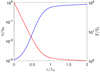 |
Fig. 3 Temperature and density profiles as a function of the dimensionless height ɀ/L0 within the loop obtained using |


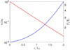 |
Fig. 4 Temperature and density profiles as in Fig. 3, obtained using |


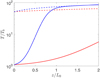 |
Fig. 5 Comparison between the temperature profiles already shown in Figs. 3 and 4 (solid curves) and the temperature profiles obtained using the same parameters but setting A = 1 (dashed curves). Blue curves refer to the case of a Sun-like corona and red curves to the case in which there is not a Sun-like corona. |
3 Application to low-mass main-sequence stars
Let us now apply our model to low-mass main-sequence stars, that is, stars with M < 1.5 M⊙, for which a Sun-like corona is expected to be present (in Appendix A we will discuss the case of larger-mass stars).
In the previous sections, we have shown that the predictions of the model only depend on two dimensionless parameters,  and
and  . Both dimensionless parameters are fixed by three star quantities, that is, the star mass M, the star radius R and the thermostat reference temperature Tb (which we identify with the typical temperature of the star’s high chromosphere), and by two quantities defining the model, that is, the loop length L and the average of temperature increments 〈ΔT〉. Using the scaling relations valid for low-mass main sequence stars (Eker et al. 2018) we can express
  and
and  in terms of M, L and 〈ΔT〉. To do so, we first use the scaling law relating the star’s radius to its mass, namely
 (13)
(13)
where R⊙ and M⊙ are the Sun’s radius and mass, respectively, a = 0.438, b = 0.479, and c = 0.075. We also use the scaling law that relates the surface temperature T of a star to its mass, that is,
![Mathematical equation: ${T \over {{T_ \odot }}} = {\left[ {{{\cal L} \over {{{\cal L}_ \odot }}}{{\left( {{R \over {{R_ \odot }}}} \right)}^{ - 2}}} \right]^{1/4}},$](/articles/aa/full_html/2025/02/aa52879-24/aa52879-24-eq39.png) (14)
(14)
where T⊙ is the surface temperature of the Sun,
 (15)
(15)
and the parameters α and d in Eq. (15) are given by
 (16)
(16)
Let us now assume that Eq. (14), valid for surface temperatures, also holds for the chromospheric temperatures at the base of the loop which we take as thermostat reference temperatures in the model, that is, Tb, so that we can write
![Mathematical equation: ${{{T_b}} \over {{T_{b, \odot }}}} = {\left[ {{{\cal L} \over {{{\cal L}_ \odot }}}{{\left( {{R \over {{R_ \odot }}}} \right)}^{ - 2}}} \right]^{1/4}},$](/articles/aa/full_html/2025/02/aa52879-24/aa52879-24-eq42.png) (17)
(17)
where Tb,⊙ is the reference thermostat temperature for the Sun, that is, Tb,⊙ = 104 K, and ℒ/ℒ is given by Eq. (15). In Fig. 6, Tb is plotted as a function of M/M⊙. Using Eqs. (13), (15) and (17) we can write the dimensionless parameter  for a generic star as a function of the mass M of the star:
![Mathematical equation: $\Delta \tilde T = {{\langle \Delta T\rangle } \over {{T_{b, \odot }}}}{10^{ - d/4}}{\left( {{M \over {{M_ \odot }}}} \right)^{ - \alpha /4}}{\left[ {a{{\left( {{M \over {{M_ \odot }}}} \right)}^2} + b\left( {{M \over {{M_ \odot }}}} \right) + c} \right]^{1/2}}.$](/articles/aa/full_html/2025/02/aa52879-24/aa52879-24-eq44.png) (18)
(18)
From now on, we fix the value of the average temperature increment in Eq. (18) to the one we used to produce the plots on Figs. 3, 4 and 5, that is, 〈∆T〉 = 9 × 10⁵ K. The reason for this choice is that with such a value we have a million-Kelvin corona in the case of the Sun, as shown by Barbieri et al. (2024a,b). We shall nonetheless discuss the effects of varying 〈∆T〉 together with the physical limitation of this assumption later, in Sect. 3.2. Finally, using Eqs. (13) and (17) we express the stratification parameter  in terms of the mass M of the star and of the loop height zt as
 (19)
(19)
where the function ℬ is
![Mathematical equation: ${\cal B}\left( {{M \over {{M_ \odot }}}} \right) = {10^{ - d/4}}{\left( {{M \over {{M_ \odot }}}} \right)^{1 - {\alpha \over 4}}}{\left[ {a{{\left( {{M \over {{M_ \odot }}}} \right)}^2} + b\left( {{M \over {{M_ \odot }}}} \right) + c} \right]^{ - 1/2}}$](/articles/aa/full_html/2025/02/aa52879-24/aa52879-24-eq47.png) (20)
(20)
and the constant α⊙ is given by
 (21)
(21)
A plot of  as a function of M/M⊙ for a fixed value of zt is shown in Fig. 7.
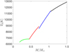 |
Fig. 6 Reference temperature of the thermostat (chromosphere), Tb in Kelvin, as a function of the mass M (in units of solar mass M⊙). The green curve corresponds to the mass interval 0.179 < M/M⊙ < 0.45, the red curve to 0.45 < M/M⊙ < 0.72, the blue curve to 0.72 < M/M⊙ < 1.05 and finally the black one to 1.05 < M/M⊙ < 1.5. |
3.1 Presence of a Sun-like corona
To understand whether the model predicts a Sun-like corona for low-mass main-sequence stars, in Fig. 8 we plot the values of the quantity X defined in Eq. (12) as a function of zt /R and M/M⊙.
In defining the model we made the approximation of constant gravity, that is, of a gravity force equal to the value at the surface of the star throughout the loop. In order for this approximation to be reasonable, we chose to consider values of zt such that zt /R ≤ 0.1. The transition between the two regimes, with and without a Sun-like hot corona, is marked by the red line corresponding to the threshold value X = 0.9 in Fig. 8.
Figure 8 shows that, according to the model, all low-mass main-sequence stars have a million-degree, Sun-like corona, because coronal conditions are met whenever one gets sufficiently high in the star’s atmosphere. For solar masses, zt/R > 0.01 is sufficient to have a million-degree corona, and this minimum height gets smaller for smaller masses, reaching zt/R > 0.0045 when M = 0.179 M⊙.
Inspection of Figure 8 shows that it is ‘easier’ to have a Sun-like corona as the mass decreases, until M = 0.5 M⊙; for smaller masses, this trend reverses. This is a consequence of the fact that larger values of  favour the presence of a Sunlike corona and indeed
  rapidly increases passing from 1.5 M⊙ to 0.5 M⊙, and then starts decreasing for smaller masses, as can be seen in Figure 7. In all the mass regime the minimum height to reach coronal conditions (that is, such that X > 0.9) is always much smaller than 0.1 R; therefore, the approximation of constant gravity is well justified.
In order to show how the density and temperature profiles depend on M, we set zt/R = 1/35, that is, a value such that X > 0.9 for any value of M, and we plot in Figure 9 the temperature T (in Kelvin) and the density n (in units of the density n0 at the base of the loop) as a function of the height z within the loop (in units of L0 = L/π, as in Figs. 3 and 4). Figure 9 shows that although the temperature at the base of the loop increases with the mass M of the star (as implied by Eqs. (14) and (17) and shown in Fig. 6) the temperature at the top is about one million degrees for all the values of M ; this is due to the fact that the ‘cold’ particles are gravitationally filtered out in the corona, leaving only the ‘hot’ particles generated by the temperature increments at ∆ T = 9 × 10⁵ K. Moreover, Figure 9 shows that for low-mass stars the rapid increase of temperature becomes steeper and steeper as the mass of star M decreases. This can be understood by looking at Fig. 8. The red level curve corresponding to the threshold X = 0.9 moves towards smaller values of zt as the mass of the star decreases and the level curves of X become denser. As a consequence,  increases as M decreases, as we already noted above. Equation (4) in turn implies that as
  increases, the population of ‘cold’ particles thermally distributed at the mean chromospheric temperature Tb is more and more exponentially depressed with height z. Therefore, by increasing the value of
  we expect an increasingly steep rapid increase of temperature. The density profile is anti-correlated with that of the temperature for all the values of M. The coronal density (in units of the density at the base of the loop, n0) decreases with M, again because
  increases: given the density at the base, by increasing the value of
  fewer and fewer particles can reach the top of the loop, and the coronal density decreases. This notwithstanding, the density drop in the corona with respect to the density at the base of the loop is never much larger than that on the Sun, being between three and four orders of magnitudes.

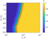 |
Fig. 8 Contour plot of X as defined in Eq. (12), computed for low-mass stars (that is, M ∈ [0.179 M⊙,1.5 M⊙]). X is plotted as a function of the star mass M in units of solar mass M⊙ and of the top height of the loop zt scaled by the star radius R. The red line corresponds to X = 0.9, the threshold separating the regime without a Sun-like corona (X < 0.9, bluish colours) from that where there is a Sun-like corona (X > 0.9, yellowish colours). |
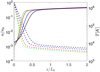 |
Fig. 9 Density n (in units of the density at the base of the loop, n0 = n(z = 0)) and temperature T (in Kelvin) as a function of the height z within the loop, scaled by L0 = L/π (where 2L is the loop length), for some values of the mass in the range 0.179 < M/M⊙ < 1.5. Here we choose zt/R = 1/35, such that X > 0.9 for all the values of M and there always is a Sun-like corona. Solid lines correspond to temperatures and dashed lines to densities. The green curves are computed for a star with mass M = 0.3 M⊙, the red ones for M = 0.6 M⊙, the blue ones for M = 0.8 M⊙ and the black ones for M = 1.2 M⊙. |
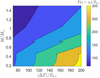 |
Fig. 10 Contour plot of the temperature at the top of the loop T(z = zt) scaled by the chromospheric temperature of the Sun Tb,⊙ = 104K as a function of the dimensionless intensity of the temperature increments ∆T scaled by the chromospheric temperature of the Sun Tb,⊙ and of the star mass scaled by the Sun mass M/M⊙. The range of ∆T goes from 70Tb,⊙ smaller than 90Tb,⊙ (that is the value used in the case of the Sun) up to 200Tb,⊙ larger than the value used for the Sun. For the ratio zt/R we have used 1/35 that is the same value used in the previous section. |
3.2 Amplitude of temperature fluctuations
Throughout our previous discussion we have set the parameter 〈∆T〉 = 〈∆T⊙〉 = 9 × 10⁵ K in order to produce a Sun-like corona. Anyhow, as already mentioned, our mechanism is supposed to have a magnetic origin. Because of this, the intensity of the temperature increments 〈∆T〉 might depend on the strength of the magnetic field. Stars with a lighter mass than that of the Sun have more active dynamo mechanisms and a stronger magnetic field: we can thus expect a larger 〈∆T〉 with respect to that of the Sun. In fact, these stars are known to have higher coronal temperatures (Johnstone et al. 2015) and our model does predict such a behaviour, as illustrated in the following. In Fig. 10 we report a contour plot of the temperature at the top of the Loop T(z = zt) as a function of the stellar mass and of the intensity of the temperature increments 〈∆T〉 for the same value of the ratio zt/R = 1/35 used in the previous section1. As shown in the figure, if 〈∆T〉 increases when the mass ratio M/M⊙ decreases, the model predicts larger coronal temperatures T(z = zt) for stars lighter than the Sun. This notwithstanding, one may wonder whether the values of the average temperature fluctuations only settle the coronal temperature or influence also other properties of the coronal temperature and density profiles. To answer this question, in Fig. 11 we plot X as a function of  and
and  ; the latter is the dimensionless parameter directly related to 〈∆T〉, see Eq. (18). We consider over three decades of
  , showing that the specific value of
  does not strongly affect the transition between the region where X < 0.9 (so that no Sun-like temperature profile is present) and the region where X > 0.9 (where we have a Sun-like rapid increase of temperature and a corona). The threshold between the two regions, marked by the red curve in Fig. 11, stays almost constant as a function of
  in a range of
  values that includes the maximum value of
  for low-mass stars. Maximum of
  has been evaluated from Eq. (19) within the range of M and zt considered above. Therefore, the specific value of
  does not have a strong impact on the qualitative properties of the temperature profiles.
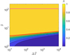 |
Fig. 11 Contour plot of X computed using Eq. (12) as a function of the dimensionless intensity of the temperature increments |


3.3 Relaxation and fluctuation timescales
The model is valid only if the timescales of the fluctuating thermostat are fast enough to prevent the coronal plasma from relaxing towards a thermal equilibrium state, that is, if conditions (1) are satisfied. However, these timescales depend on the mass of the star. For a given main-sequence star of mass M, the relaxation time tr is still defined by Eq. (2), with tT now given by
 (22)
(22)
and t𝑔 by
 (23)
(23)
where tT,⊙ and tg,⊙ are the thermal and gravitational crossing times for the case of the Sun and we have assumed, as above, 〈∆T〉 = 〈∆T⊙〉. Using L⊙ = π × 109 cm (typical for coronal loops in the Sun’s atmosphere) and 〈∆T⊙〉 = 9 × 10⁵ K, as done by Barbieri et al. (2024a), to calculate the relaxation timescale for the Sun as ![Mathematical equation: ${t_{{r_ \odot }}} = \min \left[ {{t_{{T_ \odot }}},{t_{{g_ \odot }}}} \right]$](/articles/aa/full_html/2025/02/aa52879-24/aa52879-24-eq72.png) we obtain
we obtain  . For low-mass main-sequence stars, considering the same range of values of zt as in Fig. 8, we get
  . Therefore, we obtain values of the relaxation time between 1 s and 70 s, that is, within two orders of magnitude from those of the Sun for all low-mass main-sequence stars.
4 Conclusions and perspectives
We have investigated the role of stochastic temperature fluctuations in the high chromosphere in shaping the temperature and density profiles of the coronae of main-sequence stars. We have used a model of a plasma atmosphere confined by the magnetic field (that is, made up of coronal loops) in thermal contact with the chromosphere, the latter being modelled as a thermostat with fluctuating temperature. This model was recently put forward by Barbieri et al. (2024a,b) and has already been applied to the solar atmosphere, successfully reproducing its inverted density and temperature profiles. In this model, stochastic temperature fluctuations at the base of the loop structures produce a non-thermal population of ‘hot’ and fast particles that can climb the gravity well and form the corona. On the contrary, ‘cold’ particles that are thermally distributed at the mean chromospheric temperature mostly stay close to the base of the loop structures. The rapid increase of temperature is where the two populations coexist, with a relative abundance strongly depending on the height above the surface of the star. We applied the above formalism to the case of low-mass main-sequence stars, where we expect that a corona may form out of stationary loops and therefore our model should be applicable (the case of larger-mass main- sequence stars is addressed in Appendix A). We have shown that the model always predicts inverted temperature and density profiles with a rapid increase of temperature and a corona for all main-sequence stars. Furthermore, the model predicts a rapid increase in temperature that becomes steeper as the mass of the star M decreases.
According to our collisionless model, the transition height between the cold and hot layers of the star’s atmosphere is solely determined by the stratification parameter  , that is, the ratio between the gravitational and the thermal energy of the cold population: the stronger
  , the more efficient is the energy filtration induced by the gravitational well, and the narrower is the transition height between the two layers. Since
  is only a function of the mass of the star (M), the size of the transition is completely set by the latter.
However, although not so frequent, collisions between particles do occur in the solar corona (Aschwanden 2005), so one may wonder whether a global thermalisation of the system may occur well before the hot population originating from the cold layers reaches the solar corona. First, we should note that because the mean free path scales as v4, collisions will affect the cold particles more efficiently than the hotter ones, which will experience very few collisions during their journey to the corona. For example, particles originating from heating events at 1 MK impinging on the dense solar chromosphere at 109 particles/cm3 have a mean free path of about 300 km, meaning that they will experience only a few collisions (about 5) while crossing the transition between the two layers, which is about 1500 km wide in our model. Moreover, in the actual Sun atmosphere the width of the transition region is even smaller (about 200 km) meaning that the collisionless assumption of our model is not so extreme. The same holds if we consider less massive stars where, as seen in the previous section, we except a larger ∆T implying an even larger mean-free-path. Finally, it has been shown that for typical temperatures and densities values of the transition region and low solar corona non-thermal features will persist once taking into account the collisions between particles (Shoub 1983; Dorelli & Scudder 1999; Landi & Pantellini 2001).
It has been argued that the v4 dependence of the mean-free path acts as a filter for the less energetic particles, thus providing a sharper temperature gradient which turns out to reduce the size of the transition region between the chromosphere and the solar corona in a non-thermal plasma (Landi & Pantellini 2001). Such an interplay between velocity filtration and Coulomb collisions filtering should be included in the model presented here, and it will be the subject of future work.
As a further possible development, we note that the atmospheres of stars are not static, but evolve in the form of stellar winds (Parker 1958). For this reason, an extension of our modelling to the case of open geometry could be interesting. The exospheric approach (Chamberlain 1960; Jockers 1970; Lemaire & Scherer 1971; Lamy et al. 2003; Maksimovic et al. 1997; Zouganelis et al. 2004), which explains the formation of a stellar wind as a collisionless evaporation from a given altitude, seems the relevant one for the extension of our work: indeed, using the same formalism of the present work, it might be possible to build an exospheric model having its base in the high chromosphere and able to reproduce not only the plasma of the rapid increase of temperature and of the corona but also the stellar wind.
Acknowledgements
We thank an anonymous referee for their very helpful comments. We wish to thank Germano Sacco and Elena Pancino for a careful reading of the manuscript and for very useful comments that helped us to improve our work. We acknowledge partial financial support from the Solar Orbiter/Metis program supported by the Italian Space Agency (ASI) under the contracts to the National Institute of Astrophysics (INAF), Agreement ASI-INAF N.2018- 30-HH.0. This research was partially funded by the European Union – Next Generation EU – National Recovery and Resilience Plan (NRRP) – M4C2 Investment 1.4 – Research Programme CN00000013 ‘National Centre for HPC, Big Data and Quantum Computing’ – CUP B83C22002830001 and by the European Union – Next Generation EU – National Recovery and Resilience Plan (NRRP)– M4C2 Investment 1.1 – PRIN 2022 (D.D. 104 del 2/2/2022) – Project ‘Modeling Interplanetary Coronal Mass Ejections’, MUR code 31. 2022M5TKR2, CUP B53D23004860006. Views and opinions expressed are however those of the author(s) only and do not necessarily reflect those of the European Union or the European Commission. Neither the European Union nor the European Commission can be held responsible for them. L.B. wants to thank the Sorbonne Université in the framework of the Initiative Physique des Infinis for financial support.
Appendix A Application to high-mass main-sequence stars (M > 1.5 M⊙)
In the previous Sections we have considered the case of low- mass main-sequence stars, that is, stars whose mass M is smaller than 1.5 M⊙. As discussed in the Introduction, the case of larger- mass main-sequence stars is different because these stars lack a convective region below the photosphere and therefore should not have a solar-like magnetic field able to support a stationary corona: an X-ray emission from these stars, which is indeed detected, is not attributed to a Sun-like coronal activity. Moreover, the model we applied to low-mass main-sequence stars assumes from the outset the presence of stationary coronal loops, and therefore may not be applicable as such to cases where there are no stationary magnetic configurations able to support these loops. This notwithstanding, it is interesting to study what are the predictions of the model in the case M > 1.5 M⊙, because it turns out that density and temperature profile exhibit a richer behaviour than in the low-mass case, and this may provide some hints as to possible generalisations of the model able to encompass also the case of massive stars.
In close analogy to what we have done in Sect. 3, we assume that the relation between the surface temperature T of a star and its mass M is also applicable to the chromospheric temperature, which we identify with the reference temperature of the thermostat Tb. Using the scaling relations valid for high-mass main-sequence stars given by Eker et al. (2018) for 1.5 M⊙ ≤ M ≤ 31 M⊙ we find that Tb is an increasing function of M, as for low-mass stars, although in this case the range of values of Tb is larger because the range of masses is larger, as shown in Fig. A.1, where Tb is plotted against M/M⊙. Using the abovementioned relation we can write the dimensionless parameter  for a generic star in terms of M using its definition given in Eq. (11) and fixing the mean value of the temperature increments to 〈∆T〉 = 9 × 10⁵ K. Using also the relation between the radius R and the mass M, again given by Eker et al. (2018), we can express
  in terms of M and of the loop height zt. The result is shown in Fig. A.2, for the same fixed value of zt used in Sect. 3: at variance with the case of low-mass stars,
  is now an increasing function of M. This result implies that in the case of high-mass main-sequence stars a Sun-like corona is more readily achievable as the mass increases, as shown in Fig. A.3, where the quantity X, as defined in Eq. (12), is plotted as a function of zt /R and M/M⊙, analogously to what done in Fig. 8 for the case of low- mass stars. Apart from this, Fig. A.3 shows that the model would predict a Sun-like corona even in the high-mass case and for all the range of masses considered. More interesting differences with respect to the low-mass case show up when we look directly at the temperature and density profiles, reported in Fig. A.4 for three choices of M in the high-mass range and for zt = R/35, a choice ensuring that there is a Sun-like corona. Comparing Fig. A.4 with Fig. 9 we first notice that not only the temperature at the base of the loop increases with M (as it happened for low-mas stars, and the larger variation of T at z = 0 with respect to the low-mass case is only due to the larger variation of mass, as shown in Fig. A.1), but also the temperature at the top of the loop increases, at variance with the low-mass case. For high-mass stars, the temperature at the top of the loop increases from 7 × 10⁵ K to 3 × 10⁶ K when M varies from 2 M⊙ to 25 M⊙, while it remained around 106 K in the low-mass case: this means that for high masses the temperature in the upper corona is no longer totally specified by the value of 〈∆T〉 (remember that the latter quantity has been fixed to 〈∆T〉 = 9 × 10⁵ K). At the same time, if it is true that Tb increases with M up to values of about 2.5 × 10⁵ K for M/M⊙ = 30, such a contribution is not enough to explain such growth. The second difference between the high- mass and low-mass case is that in the latter the density profiles are all very similar to each other and depend monotonically on M, the density drop being smaller for heavier stars (see Fig. 9), while the density profiles of high-mass stars reported in Fig. A.4 are different from each other and their features do not monotonically depend on M: the density drop in the upper corona is smaller for the intermediate mass case, and the density profile in the upper corona is steeper in the larger mass case with respect to the other two masses considered. A third difference is that the width of the rapid increase of temperature gets smaller when increasing M; but if the latter feature is again a consequence of the already noted fact that
  increases with M at variance with the low-mass case, the previous two differences are less easily explained. In order to explain these differences we report in Fig. A.5 the following parameter
 (A.1)
(A.1)
which is a measure of the strength of the gravitational bond (gravitational energy) with respect to the typical thermal energy of a coronal particle. As M increases, such a quantity grows and it is harder for particles to reach the top of the coronal loop. As a consequence, the velocity filtration mechanism is stronger and it produces a higher temperature in corona, much larger than the contribution of the cold population. The behaviour of the density can be still understood in terms of the parameter in Eq. A.1. In Fig. A.6 we plot the density profiles already shown in Fig. A.4 (solid curves), together with the contribution to the density of the ‘hot’ population (dashed curves). For relatively low masses the contribution to the total density of such a population is small and dominates only in the upper part of the loop, decreasing smoothly because of the small value of  . For intermediate values of the masses the contribution of the ‘hot’ population to the total density increases and we observe an increase in the density in the top of the loop. When the mass of the star becomes very high the contribution of the ‘hot’ population to the total density still increases but now the gravitational bond is so strong that the density in the loop decreases very rapidly and the density at the top of the loop becomes smaller than those observed for small and intermediate values of the star mass.
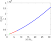 |
Fig. A.1 Plot of the thermostat (chromosphere) temperature, Tb in Kelvin, as a function of the mass M (in units of solar mass M⊙). The green curve corresponds to the mass interval 1.5 < M/M⊙ < 2.4, the red curve to 2.4 < M/M⊙ < 7, the blue curve to 7 < M/M⊙ < 31. |
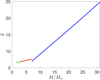 |
Fig. A.2 Same as Fig. A.1 but for the stratification parameter |

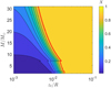 |
Fig. A.3 Contour plot of X as defined in Eq. (12), computed for high- mass stars (that is, M ∈ [1.5 M⊙, 31 M⊙]). X is plotted as a function of the star mass M in units of solar mass M⊙ and of the top height of the loop zt scaled by the star radius R. As in Fig. 8, the red line corresponds to X = 0.9, the threshold separating the regime without a Sun-like corona (X < 0.9, bluish colours) from that where there is a Sun-like corona (X > 0.9, yellowish colours). |
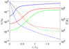 |
Fig. A.4 Density n (in units of the density at the base of the loop, n0 = n(z = 0)) and temperature T (in Kelvin) as a function of the height z within the loop, scaled by L0 = L/π (where 2L is the loop length), for some values of the mass in the range 1.5 < M/M⊙ < 31. As in Fig. 9, here we choose zt/R = 1/35, such that X > 0.9 for all the values of M and there always is a Sun-like corona. Solid lines correspond to temperatures and dashed lines to densities. The green curves are computed for M = 2 M⊙, the red ones for M = 7 M⊙, the blue ones for M = 25 M⊙. |
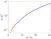 |
Fig. A.5 Stratification parameter |


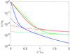 |
Fig. A.6 Comparison between the density profiles already shown in Fig. A.4 (solid curves) and those obtained by considering only the ‘hot’ population, that is, by retaining only the last term in the Eq. (4). Colours are as in Fig. A.1. |
References
- Airapetian, V. S., Jin, M., Lüftinger, T., et al. 2021, ApJ, 916, 96 [NASA ADS] [CrossRef] [Google Scholar]
- Aschwanden, M. J. 2005, Physics of the Solar Corona. An Introduction with Problems and Solutions, 2nd edn. [Google Scholar]
- Barbieri, L., Casetti, L., Verdini, A., & Landi, S. 2024a, A&A, 681, L5 [NASA ADS] [CrossRef] [EDP Sciences] [Google Scholar]
- Barbieri, L., Papini, E., Di Cintio, P., et al. 2024b, J. Plasma Phys., 90, 905900511 [NASA ADS] [CrossRef] [Google Scholar]
- Belmont, G., Grappin, R., Mottez, F., Pantellini, F., & Pelletier, G. 2013, Collisionless Plasmas in Astrophysics (Wiley) [CrossRef] [Google Scholar]
- Berghmans, D., Auchère, F., Long, D. M., et al. 2021, A&A, 656, L4 [NASA ADS] [CrossRef] [EDP Sciences] [Google Scholar]
- Chamberlain, J. W. 1960, ApJ, 131, 47 [Google Scholar]
- Dere, K. P., Bartoe, J. D. F., & Brueckner, G. E. 1989, Sol. Phys., 123, 41 [Google Scholar]
- Dmitruk, P., & Gomez, D. O. 1997, ApJ, 484, L83 [NASA ADS] [CrossRef] [Google Scholar]
- Dorelli, J. C., & Scudder, J. D. 1999, Geophys. Res. Let., 26, 3537 [NASA ADS] [CrossRef] [Google Scholar]
- Eker, Z., Bakis¸, V., Bilir, S., et al. 2018, MNRAS, 479, 5491 [NASA ADS] [CrossRef] [Google Scholar]
- Fisher, G. H., Longcope, D. W., Metcalf, T. R., & Pevtsov, A. A. 1998, ApJ, 508, 885 [CrossRef] [Google Scholar]
- Golub, L., & Pasachoff, J. M. 2009, The Solar Corona, 2nd edn. (Cambridge: Cambridge University Press) [Google Scholar]
- Gudel, M. 2004, A&AR, 12, 71 [Google Scholar]
- Gudiksen, B. V., & Nordlund, Å. 2005, Astrophys. J., 618, 1020 [NASA ADS] [CrossRef] [Google Scholar]
- Heyvaerts, J., & Priest, E. R. 1983, A&A, 117, 220 [NASA ADS] [Google Scholar]
- Howson, T. A., De Moortel, I., & Reid, J. 2020, A&A, 636, A40 [NASA ADS] [CrossRef] [EDP Sciences] [Google Scholar]
- Ionson, J. A. 1978, Astrophys. J., 226, 650 [NASA ADS] [CrossRef] [Google Scholar]
- Jockers, K. 1970, A&A, 6, 219 [NASA ADS] [Google Scholar]
- Johnstone, C. P., Güdel, M., Brott, I., & Lüftinger, T. 2015, A&A, 577, A28 [NASA ADS] [CrossRef] [EDP Sciences] [Google Scholar]
- Klimchuk, J. A. 2006, Sol. Phys., 234, 41 [Google Scholar]
- Lamy, H., Pierrard, V., Maksimovic, M., & Lemaire, J. F. 2003, J. Geophys. Res. (Space Phys.), 108, 1047 [NASA ADS] [CrossRef] [Google Scholar]
- Landi, S., & Pantellini, F. G. E. 2001, A&A, 372, 686 [NASA ADS] [CrossRef] [EDP Sciences] [Google Scholar]
- Lemaire, J., & Scherer, M. 1971, J. Geophys. Res., 76, 7479 [Google Scholar]
- Maksimovic, M., Pierrard, V., & Lemaire, J. F. 1997, A&A, 324, 725 [NASA ADS] [Google Scholar]
- Maoz, D. 2007, Astrophysics in a Nutshell, 1st edn. (Princeton, NJ: Princeton University Press) [Google Scholar]
- Molnar, M. E., Reardon, K. P., Chai, Y., et al. 2019, Astrophys. J., 881, 99 [NASA ADS] [CrossRef] [Google Scholar]
- Ness, J.-U., Güdel, M., Schmitt, J. H. M. M., Audard, M., & Telleschi, A. 2004, A&A, 427, 667 [NASA ADS] [CrossRef] [EDP Sciences] [Google Scholar]
- Nicholson, D. R. 1983, Introduction to Plasma Theory (Wiley) [Google Scholar]
- Pallavicini, R. 1989, A&R, 1, 177 [NASA ADS] [Google Scholar]
- Pannekoek, A. 1922, Bull. Astr. Inst. Netherlandd, 1, 107 [NASA ADS] [Google Scholar]
- Parker, E. N. 1958, Astrophys. J., 128, 664 [CrossRef] [Google Scholar]
- Parker, E. N. 1972, ApJ, 174, 499 [NASA ADS] [CrossRef] [Google Scholar]
- Parnell, C. E., & De Moortel, I. 2012, Philos. Trans. Roy. Soc. Lond. Ser. A, 370, 3217 [NASA ADS] [Google Scholar]
- Peter, H., Tian, H., Curdt, W., et al. 2014, Science, 346, 1255726 [Google Scholar]
- Pevtsov, A. A., Fisher, G. H., Acton, L. W., et al. 2003, ApJ, 598, 1387 [Google Scholar]
- Pontieu, B. D., Mcintosh, S. W., Carlsson, M., et al. 2011, Science, 331, 55 [NASA ADS] [CrossRef] [Google Scholar]
- Raouafi, N. E., Stenborg, G., Seaton, D. B., et al. 2023, ApJ, 945, 28 [NASA ADS] [CrossRef] [Google Scholar]
- Rappazzo, A. F., & Parker, E. N. 2013, Astrophys. J. Lett., 773, L2 [NASA ADS] [CrossRef] [Google Scholar]
- Rappazzo, F., Velli, M., Einaudi, G., & Dahlburg, R. B. 2008, Astrophys. J., 677, 1348 [NASA ADS] [CrossRef] [Google Scholar]
- Rosseland, S. 1924, MNRAS, 84, 720 [NASA ADS] [CrossRef] [Google Scholar]
- Scudder, J. D. 1992a, Astrophys. J., 398, 299 [NASA ADS] [CrossRef] [Google Scholar]
- Scudder, J. D. 1992b, Astrophys. J., 398, 319 [NASA ADS] [CrossRef] [Google Scholar]
- Shoda, M., & Takasao, S. 2021, A&A, 656, A111 [NASA ADS] [CrossRef] [EDP Sciences] [Google Scholar]
- Shoda, M., Namekata, K., & Takasao, S. 2024, A&A, 691, A152 [NASA ADS] [CrossRef] [EDP Sciences] [Google Scholar]
- Shoub, E. C. 1983, Astrophys. J., 266, 339 [NASA ADS] [CrossRef] [Google Scholar]
- Teriaca, L., Banerjee, D., Falchi, A., Doyle, J. G., & Madjarska, M. S. 2004, A&A, 427, 1065 [NASA ADS] [CrossRef] [EDP Sciences] [Google Scholar]
- Tiwari, S. K., Panesar, N. K., Moore, R. L., et al. 2019, Astrophys. J., 887, 56 [NASA ADS] [CrossRef] [Google Scholar]
- Wilmot-Smith, A. L. 2015, Philos. Trans. Roy. Soc. Lond. Ser. A, 373, 20140265 [NASA ADS] [Google Scholar]
- Yang, S. H., Zhang, J., Jin, C. L., Li, L. P., & Duan, H. Y. 2009, A&A, 501, 745 [NASA ADS] [CrossRef] [EDP Sciences] [Google Scholar]
- Zouganelis, I., Maksimovic, M., Meyer-Vernet, N., Lamy, H., & Issautier, K. 2004, Astrophys. J., 606, 542 [NASA ADS] [CrossRef] [Google Scholar]
Anyhow, we get similar results even for other values of the ratio zt /R.
All Figures
|
Fig. 1 Schematics of the loop model. The coronal plasma in the loop is treated as collisionless and in thermal contact with a fully collisional chromosphere (modelled as a thermostat). |
| In the text | |
|
Fig. 2 Sketch of the time series of the temperature of the thermostat (chromosphere). During the time intervals of duration τ the temperature increases by an amount ΔT and during the waiting times tw it returns to the typical chromospheric value Tb. |
| In the text | |
|
Fig. 3 Temperature and density profiles as a function of the dimensionless height ɀ/L0 within the loop obtained using |
| In the text | |
|
Fig. 4 Temperature and density profiles as in Fig. 3, obtained using |
| In the text | |
|
Fig. 5 Comparison between the temperature profiles already shown in Figs. 3 and 4 (solid curves) and the temperature profiles obtained using the same parameters but setting A = 1 (dashed curves). Blue curves refer to the case of a Sun-like corona and red curves to the case in which there is not a Sun-like corona. |
| In the text | |
|
Fig. 6 Reference temperature of the thermostat (chromosphere), Tb in Kelvin, as a function of the mass M (in units of solar mass M⊙). The green curve corresponds to the mass interval 0.179 < M/M⊙ < 0.45, the red curve to 0.45 < M/M⊙ < 0.72, the blue curve to 0.72 < M/M⊙ < 1.05 and finally the black one to 1.05 < M/M⊙ < 1.5. |
| In the text | |
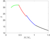 |
Fig. 7 Same as Fig. 6 but for the stratification parameter |
| In the text | |
|
Fig. 8 Contour plot of X as defined in Eq. (12), computed for low-mass stars (that is, M ∈ [0.179 M⊙,1.5 M⊙]). X is plotted as a function of the star mass M in units of solar mass M⊙ and of the top height of the loop zt scaled by the star radius R. The red line corresponds to X = 0.9, the threshold separating the regime without a Sun-like corona (X < 0.9, bluish colours) from that where there is a Sun-like corona (X > 0.9, yellowish colours). |
| In the text | |
|
Fig. 9 Density n (in units of the density at the base of the loop, n0 = n(z = 0)) and temperature T (in Kelvin) as a function of the height z within the loop, scaled by L0 = L/π (where 2L is the loop length), for some values of the mass in the range 0.179 < M/M⊙ < 1.5. Here we choose zt/R = 1/35, such that X > 0.9 for all the values of M and there always is a Sun-like corona. Solid lines correspond to temperatures and dashed lines to densities. The green curves are computed for a star with mass M = 0.3 M⊙, the red ones for M = 0.6 M⊙, the blue ones for M = 0.8 M⊙ and the black ones for M = 1.2 M⊙. |
| In the text | |
|
Fig. 10 Contour plot of the temperature at the top of the loop T(z = zt) scaled by the chromospheric temperature of the Sun Tb,⊙ = 104K as a function of the dimensionless intensity of the temperature increments ∆T scaled by the chromospheric temperature of the Sun Tb,⊙ and of the star mass scaled by the Sun mass M/M⊙. The range of ∆T goes from 70Tb,⊙ smaller than 90Tb,⊙ (that is the value used in the case of the Sun) up to 200Tb,⊙ larger than the value used for the Sun. For the ratio zt/R we have used 1/35 that is the same value used in the previous section. |
| In the text | |
|
Fig. 11 Contour plot of X computed using Eq. (12) as a function of the dimensionless intensity of the temperature increments |
| In the text | |
|
Fig. A.1 Plot of the thermostat (chromosphere) temperature, Tb in Kelvin, as a function of the mass M (in units of solar mass M⊙). The green curve corresponds to the mass interval 1.5 < M/M⊙ < 2.4, the red curve to 2.4 < M/M⊙ < 7, the blue curve to 7 < M/M⊙ < 31. |
| In the text | |
|
Fig. A.2 Same as Fig. A.1 but for the stratification parameter |
| In the text | |
|
Fig. A.3 Contour plot of X as defined in Eq. (12), computed for high- mass stars (that is, M ∈ [1.5 M⊙, 31 M⊙]). X is plotted as a function of the star mass M in units of solar mass M⊙ and of the top height of the loop zt scaled by the star radius R. As in Fig. 8, the red line corresponds to X = 0.9, the threshold separating the regime without a Sun-like corona (X < 0.9, bluish colours) from that where there is a Sun-like corona (X > 0.9, yellowish colours). |
| In the text | |
|
Fig. A.4 Density n (in units of the density at the base of the loop, n0 = n(z = 0)) and temperature T (in Kelvin) as a function of the height z within the loop, scaled by L0 = L/π (where 2L is the loop length), for some values of the mass in the range 1.5 < M/M⊙ < 31. As in Fig. 9, here we choose zt/R = 1/35, such that X > 0.9 for all the values of M and there always is a Sun-like corona. Solid lines correspond to temperatures and dashed lines to densities. The green curves are computed for M = 2 M⊙, the red ones for M = 7 M⊙, the blue ones for M = 25 M⊙. |
| In the text | |
|
Fig. A.5 Stratification parameter |
| In the text | |
|
Fig. A.6 Comparison between the density profiles already shown in Fig. A.4 (solid curves) and those obtained by considering only the ‘hot’ population, that is, by retaining only the last term in the Eq. (4). Colours are as in Fig. A.1. |
| In the text | |
Current usage metrics show cumulative count of Article Views (full-text article views including HTML views, PDF and ePub downloads, according to the available data) and Abstracts Views on Vision4Press platform.
Data correspond to usage on the plateform after 2015. The current usage metrics is available 48-96 hours after online publication and is updated daily on week days.
Initial download of the metrics may take a while.