© The Authors 2025

1 Introduction

The interaction between plasma and magnetic fields and currents affects the plasma’s dynamics in the solar atmosphere. The configuration and topology of the structures in this medium follow the characteristics of the magnetic fields, electric current sheets, and plasma evolution. Thus, studying the magnetic field and plasma characteristics plays a key role in describing the evolution and interactions between the coronal plasma structures, and the several events resulting from temporal and spatial changes in these parameters. Nevertheless, the dynamics and topology of the solar corona are mainly formed and evolved by specifying the magnetic field configuration. In the photosphere and lower chromosphere, the structures evolve by the effect of both plasma and magnetic forces to the same extent. In other words, because of the low plasma β parameter, the solar corona is a magnetic-field- dominated medium, while, other forces such as gravitational and pressure forces must be taken into account in the lower layer of the solar atmosphere (Gary 2001).

A significant number of observational instruments, earth- or space-based, are engaged in acquiring data from the magnetic field, temperature, pressure, and density in the solar environment. However, the precise determination of the magnetic field in the solar corona is currently impossible since the thermal broadening of the Zeeman lines swamps the magnetic broadening (Wiegelmann et al. 2006). Also, the optically thin condition for coronal emission creates an integrated characteristic, which makes the situation more complicated (Wiegelmann & Neukirch 2006). One way is to reconstruct the magnetic field using the data obtained by the magnetic imager instruments, such as the Helioseismic and Magnetic Imager (HMI) on the Solar Dynamic Observatory (SDO) (Schou et al. 2012; Wiegelmann et al. 2012). Several models have been developed thus far to extrapolate the magnetic field in the solar corona following the simplifying rules of force-free magnetic fields (Grad & Rubin 1958; Amari et al. 1997; Yan & Sakurai 1997, 2000). Wiegelmann & Sakurai (2021) provide a comprehensive review of the reconstruction models of force-free magnetic fields. Among these models, the optimization method, which was proposed by Wheatland et al. (2000) at first and developed by Wiegelmann (2004), received more attention. Nasiri & Wiegelmann (2019) and then Fatholahzadeh et al. (2023) applied a constrained optimization approach to calculate the NonLinear Force-Free magnetic Field (NLFFF) using the Lagrange multiplier technique. A concept of the constrained optimization principles with Lagrange multiple techniques and its application to different physical problems are briefly discussed by Bertsekas (1996), Krishna Vadlamani et al. (2020), and Polyak (1969). Most of these models reconstruct themagnetic field in a computational box located on the photosphere up to the corona. However, due to the condition of mixed β in the photosphere and lower layers of the chromosphere, the effects of nonmagnetic forces in lower parts of the computational box may cause the results to be inconsistent with real solar coronal data. We know that the magnetohydrostatic (MHS) condition, as the stable equilibria, describes the physics of the interactions between the plasma structure and magnetic field in the lower solar atmosphere. The governing equations in this respect are $$\frac{1}{{\mu }_0}(\mathbf{\nabla }\times \mathit{B})\times \mathit{B}-\mathbf{>\nabla }P-\rho \mathbf{\nabla }\psi =0,$$(1)

and $$\mathbf{\nabla }\cdot \mathit{B}=0,$$(2)

where B, P, ρ, µ₀, and ψ, are the magnetic field, plasma pressure, plasma density, vacuum permeability, and gravitational potential, respectively. Equation (1) expresses the MHS equilibria and Eq. (2) shows that the physical magnetic field must be solenoidal. Since a general solution does not exist for Eqs. (1) and (2), Low (1985) applied a semi-analytical solution to these equations (hereafter LOW). Some models were developed to reconstruct the magnetic field in the plasma by imposing a set of boundary conditions for B, P, and ρ and using extrapolation techniques. Wiegelmann & Neukirch (2006) reconstructed magnetic field in MHS equilibria by optimizing Eq. (1) and neglecting the gravitational force and by introducing a generalized pressure, which is defined to include the contributions of the plasma pressure and the energy density of the flow. Wiegelmann et al. (2007) applied an optimization approach for the computation of MHS coronal equilibria in spherical geometry. In another approach, Gilchrist & Wheatland (2013), and Gilchrist et al. (2016a) used the Grad-Rubin method to extrapolate the magnetic field for MHS equilibria. Wiegelmann et al. (2015) developed MHS modeling of the solar atmosphere using real data from the Sunrise/IMaX instrument. Zhu & Wiegelmann (2018) applied the variable transformation method to guarantee the positivity of the plasma pressure and mass density in the solar atmosphere during optimization. They extended their work by testing their model with the radiative magnetohydrodynamics simulation of a solar flare (Zhu & Wiegelmann 2019) and Sunrise/IMaX vector magnetogram data (Zhu et al. 2020). An excellent review of this issue is given by Zhu et al. (2022). Despite the development of several models to reconstruct the magnetic field, there are still shortcomings in this regard. Therefore, it is still possible to propose alternative models in this respect. One of the shortcomings is that the reconstruction of the magnetic field considering MHS equilibria is significantly slower than the NLFFF (Zhu et al. 2022; Gilchrist et al. 2016b). So it is useful to achieve methods that are computationally more efficient. In the case of the MHS optimization models, other shortcomings are the sensitivity to the boundary conditions and the requirement of high-resolution observational data (Zhu et al. 2022). As an extension of our previous work (Fatholahzadeh et al. 2023), for this work we tried to reconstruct the magnetic field considering the plasma parameters in the MHS environment employing the Lagrange multiplier technique to develop a constrained optimization model.

In Section 2, the theory of constrained optimization of the MHS model is presented and an appropriate Lagrangian is introduced considering Eqs. (1) and (2). In Section 3, a brief review of the comparison model and the reference solution is provided. In Section 4, a method for employing boundary conditions is described, and the numerical calculation and algorithm are introduced. In Section 5, the results are presented and compared with those of the comparison model. Finally, Section 6 is devoted to concluding remarks.

2 Constrained optimization theory

The optimization models are easy to implement and have the advantage of computational efficiency. In these methods, an appropriate Lagrangian is suggested to reconstruct a magnetic field based on the relevant equilibrium equations. The present model is an extension of the constrained optimization with the vector Lagrange multiplier (COV) introduced in Fatholahzadeh et al. (2023). We employed Eq. (2) as the governing equation of solenoidal nature, and Eq. (1) as the constraint equation fixing the MHS nature of the magnetic field and plasma distribution. Then, to minimize the objective term |∇ ⋅ B| subject to the constraint equation $\frac{1}{{\mu }_0}(\mathbf{\nabla }\times B)\times B-\mathbf{\nabla }P-\rho \mathbf{\nabla }\psi =0$, the magnetic field and plasma parameters were obtained. To reconstruct the field over an active region, we assumed a computational box whose lower side coincides with the given magnetogram, while the lateral and top sides are in the solar atmosphere. For the third term of Eq. (1), one can substitute $\rho \mathbf{\nabla }\psi =\rho g\widehat{ɀ}$, where ɡ is the gravitational acceleration perpendicular to the photosphere. Thus, the corresponding Lagrangian is $$\begin{array}{l}L=L_D+L_M={\displaystyle {\int }_v{\omega }_D}|\mathbf{\nabla }\cdot B{|}^2\text{d}v\\ +{\displaystyle {\int }_v{\omega }_M}(\mathit{\lambda }\cdot [(\mathbf{\nabla }\times B)\times B-\mathbf{\nabla }P-\rho g\widehat{ɀ}])\text{d}v,\end{array}$$(3)

where ω_D and ω_M are weighting functions, and indices D and M refer to divergence-free and MHS, respectively. The λ ≡ λ(x, y, ɀ, t) denotes the vector Lagrange multiplier due to the vector behavior of the constraint equation in Lagrangian. The dimension of the integrand in the first term in Eq. (3) is $\frac{B^2}{l^2}$, and that of the constraint equation is $\frac{B^2}{l}$, where l has the dimension of length. Therefore, the dimensional analysis shows |λ| to have dimension $\frac{1}{l}$.

It is obvious that Eqs. (1) and (2) are satisfied if L = 0. Taking the derivative of Eq. (3) and using appropriate vector algebra, one may obtain $$\begin{array}{l}\frac{\partial L}{\partial t}={\displaystyle {\int }_v\left[\frac{\partial B}{\partial t}\cdot F_B+\frac{\partial \mathit{\lambda }}{\partial t}\cdot F_{\lambda }+\frac{\partial P}{\partial t}\cdot F_P+\frac{\partial \rho }{\partial t}\cdot F_{\rho }\right]}\mathrm{\hspace{0.17em}d}v\\ +{\displaystyle {\int }_s\left[\frac{\partial B}{\partial t}\cdot G_B+\frac{\partial P}{\partial t}\cdot G_P\right]}\mathrm{\hspace{0.17em}d}s,\end{array}$$(4)

where $$\begin{array}{l}{F}_{B(\mathit{B},\mathit{\lambda },P,\rho )}={\omega }_M(\lambda \times (\mathbf{\nabla }\times B))+(\mathbf{\nabla }\times (B\times \lambda ))\\ -(B\times \lambda )\times \mathbf{\nabla }{\omega }_M\mathbf{-}2\left[{\omega }_D\mathbf{\nabla }(\mathbf{\nabla }\cdot B)+\left(\mathbf{\nabla }{\omega }_D\right)(\mathbf{\nabla }\cdot B)\right],\end{array}$$(5) $$F_{\mathit{\lambda }(B,\mathit{\lambda },P,\rho )}={\omega }_M(\mathit{\lambda }\cdot [(\mathbf{\nabla }\times B)\times B-\mathbf{\nabla }P-\rho g\widehat{ɀ}]),$$(6) $${\mathit{F}}_{P(B,\mathit{\lambda },P,\rho )}={\omega }_M(\mathbf{\nabla }\cdot \mathit{\lambda })-\mathit{\lambda }\cdot \left(\mathbf{\nabla }{\omega }_d\right),$$(7) $${\mathit{F}}_{\rho (B,\mathit{\lambda },P,\rho )}=-{\omega }_M(\mathbf{\nabla }\cdot g\widehat{ɀ}),$$(8) $${\mathit{G}}_{\mathit{B}}(\mathit{B},\mathit{\lambda },P,\rho )={\omega }_M[(\mathit{B}\times \mathit{\lambda })\times \widehat{\mathit{n}}]+{\omega }_D(\mathbf{\nabla }\mathit{\cdot }\mathit{B})\widehat{\mathit{n}},$$(9)

and $${\mathit{G}}_{P(\mathit{B},\mathit{\lambda },P,\rho )}={\omega }_M(\widehat{\mathit{n}}\cdot \mathit{\lambda }).$$(10)

Details of the above calculations are given in Appendix A. Assuming that no active region is located near the edges of the magnetogram, and that the lateral sides of the computational box are located in a quiet region, one may assume that the magnetic field and plasma pressure would remain constant on the boundary surfaces throughout the optimization procedure, that is, $${\left(\frac{\partial \mathit{B}}{\partial t}\right)}_s=0,\text{ and }{\left(\frac{\partial \mathit{P}}{\partial t}\right)}_s=0.$$(11)

Therefore, the surface integral in Eq. (4) vanishes. We reconstructed the magnetic field and computed the plasma pressure and density inside the computational box by tracing the magnetic field lines. The numerical method used to minimize the Lagrangian L is based on an iterative scheme. By starting with a positive L at the beginning, and assuming the volume integrals in Eq. (4) will always be negative, L will eventually approach zero at the end of the iteration. Thus, we assume $$\begin{array}{c}l\frac{\partial \mathit{\lambda }}{\partial t}=-{\mu }_{\lambda }{\mathit{F}}_{\lambda },\frac{\partial \mathit{B}}{\partial t}=-{\mu }_B{\mathit{F}}_B\\ l\\ l\frac{\partial P}{\partial t}=-{\mu }_P{\mathit{F}}_P,\text{ and }\frac{\partial \rho }{\partial t}=-{\mu }_{\rho }{\mathit{F}}_{\rho },\end{array}$$(12)

where µ_λ, µ_P, µ_ρ, and µ_B are positive parameters, which are assumed to be equal to one during the optimization. Using Eq. (12) in Eq. (4), one may obtain the following explicit form: $$\frac{\partial L}{\partial t}=-{\displaystyle {\int }_v\left({\mu }_{\lambda }{\left|{\mathit{F}}_{\lambda }\right|}^2+{\mu }_B{\left|{\mathit{F}}_B\right|}^2+{\mu }_P{\left|{\mathit{F}}_P\right|}^2+{\mu }_{\rho }{\left|{\mathit{F}}_{\rho }\right|}^2\right)}\text{d}v,$$(13)

which is obviously negative. By the inherent property of the optimization method, one may choose any arbitrary λ, B, P, and ρ as an initial input, and follow their evolution through the coupled Eq. (12) to find the set of parameters that satisfy Eq. (1). The magnetic field, plasma pressure, and density are the physical quantities that must be determined at the beginning of the optimization as initial input; however, the initial value of the Lagrange multiplier is given by a suitable ansatz in terms of B₀, P₀, and ρ₀ as $${\mathit{\lambda }}_0\equiv {\left|{\mathit{B}}_0\right|}^{-2}\left[\left(\mathbf{\nabla }\times {\mathit{B}}_0\right)\times {\mathit{B}}_0-\mathbf{\nabla }{P}_0-{\rho }_{0}g\widehat{ɀ}\right].$$(14)

Starting with a positive L at the beginning, it will eventually approach zero at the end of the iteration.

3 Comparison model and reference solutions

To check the performance of the present model, one may compare the corresponding results with those obtained by other models, and possibly with an analytical solution. To describe the equilibria, Low (1985, 1991) considered an equation of state for the plasma to relate density, pressure, and temperature, and presented a class of semi-analytic solutions of the magnetized solar atmospheres as $$\mathbf{\nabla }\times \mathit{B}={\alpha }_0\mathit{B}+f(ɀ)\nabla {\mathit{B}}_{ɀ}\widehat{ɀ}.$$(15)

Here, α₀ is the force-free parameter and f (ɀ) is an arbitrary function. Based on the nature of the solar atmosphere, f (ɀ) should be chosen in such a way that the magnetic field becomes approximately force-free as the height increases. According to Low (1991), we consider f (ɀ) = ae^−kz, where a and k are free parameters that control the nonmagnetic forces and the effective height of the Lorentz force, respectively. With these considerations, Low (1991) obtained the relation for plasma pressure and density in the terms of the magnetic field as $$P=P_0(ɀ)-\frac{1}{2{\mu }_0}f(ɀ)B_{ɀ}^2,$$(16)

and $$\rho =-\frac{1}{𝑔}\frac{ \text{d}{P}_0}{ \text{d}ɀ}+\frac{1}{{\mu }_0𝑔}\left[\frac{ \text{d}f}{ \text{d}ɀ}\frac{B_{ɀ}^2}{2}+f(B\cdot \nabla )Bɀ\right],$$(17)

where P₀(ɀ) = P₀e^−ɀ/H, and H = 1.65 × 105 km is the isothermal scale height. Low (1985) assumed P₀ = 28 × 10⁻² dyn/cm², ρ₀ = 8.35 × 10⁻¹⁶ gr/cm³, 𝑔 = 2 × 10⁴ cm/s², α₀ = −3.0, a = 0.5, and k = 0.02 and determined the plasma parameters for a given magnetic field. In our model to determine the magnetic field in the box, we used the Low & Lou (1990) solution (hereafter L&L), which assumes a point source at the origin and provides a set of axisymmetric nonlinear force-free fields. This set of semi-analytical solutions has a multi-polar character based on the depth of burying origin below the photosphere (l) and the inclination of the axis of symmetry of the fields to the normal (ϕ). The semi-analytical solutions, which are labeled in the L&L notation as P_1,1 with l = 0.3 and ϕ = π/4, were selected, and the quantities in Eq. (1) were generated for all the cells in the box.

We compared the results of the MHS constrained optimization model with those obtained by Zhu & Wiegelmann (2018), henceforth referred to as the optimization of magnetohydrostatic (OM) model. The OM model calculates the magnetic field and plasma parameters by minimizing the following Lagrangian: $$\begin{array}{l}L=\underset{v}{{\displaystyle \int }}({\omega }_b|B{|}^{-2}[(\mathbf{\nabla }\cdot \mathit{B})\mathit{B}]\hfill \\ +{\omega }_a|B{|}^{-2}\left[(\mathbf{\nabla }\times \mathit{B})\times \mathit{B}-\mathbf{\nabla }{Q}^2-\frac{R^2}{H_s}\widehat{ɀ}\right],\hfill \end{array}$$(18)

where ω_a and ω_b are the weighting functions and H_s is the pres- sure scale height. The variables P = Q² and $\rho =\frac{R^2}{g{H}_s}$ were chosen to guarantee that the plasma pressure and density remain positive during the optimization. It should be noted that for comparison of Constrained Optimization of Magnetohydrostatic using Vector Lagrange multiplier (hereafter COMV) and OM models, the initial values must be the same.

4 Algorithm

To perform the constrained optimization procedure, a computational box was chosen so that the lower side is located on the photosphere and the lateral sides are located in the quiet region of the sun. The dimensions of the box should be small enough to ignore the curvature of the solar surface. Here, we assumed the computational box over an active region and divided it into 80 segments along the x and y axes (as shown in Fig. 1), and 40 segments along the ɀ axis. The dimensions of the cubic grid cells are 40 km. Then, the following steps ware taken to reconstruct the magnetic field and calculate the plasma pressure and density in the MHS equilibrium.

1. The artificial vector magnetogram was selected and was assumed as the lower boundary of the computational box. It consists of the magnetic field components at the photosphere, which was generated by an L&L semi-analytical solution using the Runge-Kutta numerical method (Zheng & Zhang 2017; Engquist 2016).

2. Thanks to the optimization mechanism, the minimization may be done by considering any arbitrary initial value. It should be only noted that the input value must be consistent with the boundary condition and the physical specification of the model. We performed our model in which the interior of the computational box as well as the lateral and top boundaries are filled with a nonlinear force-free field as the initial state. For this purpose, we employed the COV model introduced in our previous work (Fatholahzadeh et al. 2023).

3. Since the gravitational acceleration changes only 0.447 percent in 1.6 Mm, we considered a constant value 𝑔 = 274 m/s² and solved Eqs. (1) and (2) following Section 3. However, we needed to determine the initial values for plasma parameters. To find the plasma pressure, P, in the photosphere, we used P = P_quiet − |B_ɀ|², where P_quiet = 1.228 × 10⁵ dyn/cm² is the plasma pressure in the quiet sun. Since the lateral boundaries of the box were chosen to be located in the quiet sun and no active region would lie close to the boundaries, Eq. (11) is satisfied. For this aim, we could replace the pressure values at the lateral side boundaries with the corresponding values in the quiet sun using the vertical pressure profile (Avrett & Loeser 2008). Then, we calculated the plasma pressure distribution inside the box by applying the bi-linear interpolation method (Getreuer 2011). By assuming a gravitational stratification and a vertical onedimensional temperature profile (Avrett & Loeser 2008), and using the equation of state for the ideal gas as P/ρT = k_b /m, the density could calculated for each grid cell all over the box. Fig. 1 shows the artificial magnetogram and the distribution of plasma pressure and density at the photosphere as the lower side boundary condition.

4. Finally, using Eq. (12), the vector Lagrange multiplier, λ, magnetic field, B, plasma pressure, P, and plasma density, ρ, were updated simultaneously at each iteration step inside the computational box. As the minimization process proceeded and the Lagrangian tended toward zero, we could obtain the magnetic field, plasma pressure, and density.

Fig. 1 Boundary condition at the lower side of the box. (a) The artificial magnetogram (Gauss), (b) distribution of plasma pressure (dyn/cm2), and (c) distribution of plasma density (gr/cm3). In panel (a), the arrows represent the horizontal components of the magnetic field in the photosphere$\left(B_x\widehat{i}+B_y\widehat{j}\right)$. The intensity of the radial component of the magnetic field, | Bɀ |, is displayed via the colormap.

5 Numerical analysis

Following the procedure explained in Section 4, Eq. (12) was solved and the corresponding magnetic field and plasma parameters for all grid cells were calculated and used as the initial values for optimization. The constrained optimization model was performed by choosing the force-free magnetic field as input. The plasma physical parameters needed to be matched smoothly on the boundary of the box, and to reduce the boundary mismatches, appropriate weighting functions were considered (Wiegelmann 2004). The weighting functions were assumed to vary from one to zero inside the lateral and top boundary layers determined by the thickness n_d = 8. By this assumption, the weighting functions ω_D and ω_M are equal to one inside the box and approach zero on the boundary following a harmonic profile. The results of the COMV model were compared with those of the OM model. Before discussing the comparing procedure, we provide a review the indicators defined by Schrijver et al. (2006) to compare the performance of COMV and the comparison model. These indicators are the following.

A) The relative magnetic energy, RME, shows the ability of the model to estimate the energy content of the reconstructed magnetic field, defined as $$ϵ\equiv \frac{{\displaystyle {\sum }_{i=1}^N{\left|b_i\right|}^2}}{{\displaystyle {\sum }_{i=1}^N{\left|B_i\right|}^2}},$$(19)

where, b_i and B_i denote the final magnetic field and the corresponding references field, respectively, N denotes the total number of grid points in the computational box, and i refers to the number of each cell.

B) The vector correlation, VC, represents the correlation between B_i and b_i at each grid point i, and it is defined as $$VC\equiv \frac{{\displaystyle {\sum }_{i=1}^N{B}_i}{b}_i}{\sqrt{{\displaystyle {\sum }_{i=1}^N{\left|B_i\right|}^2}{\displaystyle {\sum }_{i=1}^N{\left|b_i\right|}^2}}}.$$(20)

C) The Cauchy-Schwarz, CS, is defined based on Cauchy- Schwarz inequality to measure the angle between B_i and b_i as $$CS\equiv \frac{1}{N}{\displaystyle \sum _{i=1}^N\frac{B_i\cdot b_i}{\left|B_i\right|\left|b_i\right|}}.$$(21)

D) The normalized vector error, NVE, which approaches zero when b_i and B_i are almost identical, is defined as $$NVE\equiv {\displaystyle \sum _{i=1}^N\frac{\left|b_i-B_i\right|}{\left|B_i\right|}}.$$(22)

E) Wheatland et al. (2000) defined the fractional flux errors, f_i, to show the convergence of the solenoidal term as $$f_i=\frac{{\displaystyle {\int }_{\text{Δ}{s}_i}B}\cdot ds}{{\displaystyle {\int }_{\text{Δ}{s}_i}|}B|\text{d}s}\approx \frac{{(\nabla \cdot B)}_i\left(\text{Δ}{V}_i\right)}{B_i{A}_i}.$$(23)

These indicators actually determine how much the magnetic field corresponds to the reference one. In addition to the magnetic field, one must compare the plasma parameters such as pressure and density. Hence the following indicators that are introduced by Zhu & Wiegelmann (2018) are of interest.

F) The Pearson’s correlation, PC, that is, the ratio between covariance of the extrapolated plasma pressure, P_i, and the reference one, $P_{0_i}$, to their standard deviation, is defined as $$P{C}_P=\frac{{\displaystyle {\sum }_{i=1}^N\left(P_i-\overline{P}\right)}\left(P_{0_i}-\overline{P_0}\right)}{\sqrt{{\displaystyle {\sum }_{i=1}^N{\left(P_i-\overline{P}\right)}^2}}\sqrt{{\displaystyle {\sum }_{i=1}^N{\left(P_{0_i}-\overline{P_0}\right)}^2}}},$$(24)

and that for the plasma density is defined as $$P{C}_{\rho }=\frac{{\displaystyle {\sum }_{i=1}^N\left({\rho }_i-\overline{\rho }\right)}\left({\rho }_{0_i}-\overline{{\rho }_0}\right)}{\sqrt{{{\displaystyle {\sum }_{i=1}^N\left({\rho }_i-\overline{\rho }\right)}}^2}\sqrt{{\displaystyle {\sum }_{i=1}^N{\left({\rho }_{0_i}-\overline{{\rho }_0}\right)}^2}}},$$(25)

where $\overline{P}$ and $\overline{\rho }$ denote the mean value for pressure and density, respectively.

Here we wish to follow the model’s performance by examining the correspondence between the field lines obtained from the COMV, OM, and the reference model. To do this one may define the following indicators.

G) The R value, which shows how the MHS equilibria are fulfilled by applying the constrained optimization model, measures the degree of alignment between the nonmagnetic forces and magnetic field lines and is defined as $$R_{value}=\frac{\widehat{B}\cdot (-\nabla P+\rho \mathit{g})}{|\nabla P|+\left|\rho \mathit{g}\right|}.$$(26)

H) The C value, which measures the agreement between extrapolated and reference magnetic field lines (Wiegelmann et al. 2005), is defined as $$C_{value}=\frac{1}{l^2}{\displaystyle {\int }_0^l\sqrt{R_{ref}-R_{ext}}},$$(27)

where R is the three-dimensional space curve of the field line and integration goes along the field line by a total length of l. The subscripts ref and ext refer to the “reference” and “extrapolated” magnetic field lines, respectively.

The magnetic field reconstruction in the MHS equilibria was done and the results were obtained using the constrained optimization. In this case, the iteration procedure goes on until the criteria L_{t + 1}/L_t < 10⁻⁵ is satisfied during the numerical calculations. Therefore, the iteration was stopped at 20 000 steps. It seems that the results obtained up to this step are almost enough to compare the model’s performance. One may have a desire to continue the iteration procedure to more steps, to achieve more accurate results. However, our goal is to show the model’s performance and compare its results in the same steps with those of the comparison model. After 20 000 iteration steps, the value of L approaches ~0.0037 of its initial value (L₀) for COMV, while it approaches ~0.0111 for the OM model. The results show that the COMV model has better convergence than the OM model. The results of L/L₀ are plotted in Fig. 2 for the COMV and the OM models. It is important to note that in the optimization theory, one expects the Lagrangian to become “exactly” zero, while in the numerical calculation, the same Lagrangian “approaches” zero depending on how far the iteration steps are achieved.

Further, the indicators mentioned above and some other useful quantities are given in Table 1. The results of L_D /L_D0 tend to be 1.32 × 10⁻³ and 7.36 × 10⁻³ for the COMV and OM models, respectively, which show that the final magnetic field approaches a solenoidal state. A more detailed investigation of this issue may be done by calculating the fractional flux errors, which are small enough, ≃2.36 × 10⁻³ and ≃3.89 × 10⁻³ for the COMV and OM models, respectively.

Examining the behavior of plasma pressure against altitude, before and after the optimization may be useful. The balance between magnetic and plasma pressure varies between grid cells. In some grid cells, the magnetic (plasma) pressure may be locally much greater than plasma (magnetic) pressure. Thus, one may calculate the average pressure by integrating the local pressure over x and y for each layer. This is plotted as a function of ɀ in Fig. 3, which shows that the behavior of the pressure profile for the COMV and OM models is almost the same. In Fig. 4, the behavior of magnetic, plasma, and total pressure before and after optimization is shown. The pressure values decrease with increasing altitude. Although the mean magnetic pressure is lower than the mean plasma pressure at the same altitude, but by increasing the height, as expected, the total pressure is mostly affected by the magnetic pressure.

To clarify the issue, we investigated the behavior of the plasma β parameter. The mean β parameter was calculated in the same manner as the mean pressure and is plotted in terms of ɀ in Fig. 5. The values of mean β vary from ~2.9 in the photosphere up to ~5.2 in about 160 Km and then decrease to less than one, for the COMV model at the height of ɀ ≃ 411 Km and the OM model at the height of ɀ ≃ 407 Km. As shown in Fig. 5, the average beta at the lower layer of the chromosphere decreases to less than one. This height is about 581 km for the reference model. Furthermore, Bourdin (2017) calculated the average beta for the results obtained by Gary (2001), which reduced to less than one at the height between 400 and 500 Km.

Moreover, as can be seen from Table 1, according to Pearson’s correlation indicators, the reconstructed plasma pressure and density in the COMV model have a slightly better correlation with the Low solution compared to the OM model.

The ratio of the magnetic energy to its potential value, $\frac{E}{E_P}$, are 1.63 and 1.86 for the COMV and OM, respectively. This means that the available free magnetic energy E – E_P in this structure is around 9.19 × 10³²erg for the COMV model, and 1.25 × 10³³erg for the OM model, which are comparable to the energy of explosive events in the solar atmosphere. Of course, the RME values in Table 1 indicate that the magnetic energy in the computational box is closer to those of the reference model for the COMV compared to the OM model. In other words, the results obtained by the COMV model are more realistic than those of the OM model, which could be due to the better convergence in the same steps in the optimization procedure.

To examine the model more accurately, we investigated the magnetic field lines and compared them with the reference one. We examined all possible magnetic field lines within a 40 × 40 area from the center of the magnetogram where the active region is located. Among the 160 lines drawn in Fig. 6, 12 lines were chosen from different parts of the magnetogram in such a way as to be a good representation of the studied area. Using the Euler method (Yang 2017) to trace magnetic field lines, the C values were calculated for these lines and given in Table 2 for the COMV and OM models as well as the corresponding NLFFF. Also, the R values were calculated along field lines separately, and the average values of R along each field line are given in Table 2. According to Table 2, the results for the COMV and the OM models are approximately the same.

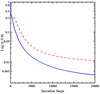Fig. 2 Iterative behavior of the normalized Lagrangian, $\frac{L}{L_0}$. The results are shown with a solid blue line for the COMV, and with a dashed red line for the OM models.

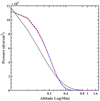Fig. 3 Behavior of the plasma pressure profile against ɀ for the COMV (solid blue line), the OM (dashed red line), and the reference (dotted black line) models.

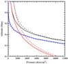Fig. 4 Comparison between the plasma pressure profile against ɀ before (dashed line) and after (solid line) optimization. The red line shows the magnetic pressure, the blue line represents the plasma pressure, and the black line shows the total pressure.

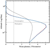Fig. 5 Behavior of the mean β parameter in terms of ɀ for the COMV (solid blue line) and the OM (dashed red line) models. The reference model is plotted in a dotted black line.

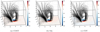Fig. 6 Reconstructed magnetic field lines plotted for (a) the COMV model, (b) the OM model, and (c) NLFFF.

6 Conclusions

Direct measurement of the magnetic field in the solar atmosphere poses numerous challenges. Although many efforts have been made to measure the magnetic field in the solar corona (Schad et al. 2024; Lin et al. 2004), one may employ the magnetic field reconstruction methods using the observational data that provide a vector magnetic field at the solar photosphere to get insight into the magnetic field in the solar atmosphere. Some authors apply a force-free magnetic field assuming a low β coronal condition. However, due to mixed plasma β conditions in the lower layers of the solar atmosphere, the force-free assumption is insufficient to describe the physical state of the MHS equilibrium, where the pressure and gravity forces cannot be neglected compared to the magnetic force. However, we present a model that uses the Lagrange multiplier technique to extrapolate the magnetic field and plasma parameters simultaneously, considering the MHS equilibria. We define a Lagrangian, where the solenoidal condition of the magnetic field serves as the objective part and incorporates the MHS equilibrium equation as the constraint using an appropriate vector Lagrange multiplier. As mentioned in Fatholahzadeh et al. (2023), “the Lagrange multiplier technique is capable of including more general cases”; here, we have shown that adding the MHS equilibrium equation as a constraint term to the Lagrangian can be considered as another case. Accordingly, a vector magnetogram was constructed using the semi-analytical solution. The pressure distribution on the photosphere was obtained by employing the balance between the magnetic and the plasma pressure. Using the bilinear method, the pressure was determined in the entire box. Considering a one-dimensional observational temperature profile, the density was calculated by the ideal gas equation of state. Then the potential magnetic field was used to obtain the NLFFF all over the box, which served to reconstruct the magnetic field in MHS equilibria. By suitable initial inputs for λ, B, P, and ρ, the iteration process was continued up to 20000 steps. The magnetic field strength, pressure, and plasma density ware revised at each step during optimization. It is essential to note that achieving an exact zero value for the Lagrangian by numerical computations is not entirely feasible; however, it is shown that the constrained optimization converges with the Lagrangian close to zero. Our results were compared with those of the OM model as well as with an analytical solution. It is found that after the 20000 iteration steps, the convergence in our model is slightly better than that of the OM model compared with the semi-analytical solutions. The relative magnetic energy indicator shows that our results are closer to those of the reference solutions and are comparable to the magnetic free energy of structures in the solar atmosphere. The plasma parameter indicators show that the reconstructed plasma pressure and density in our model are slightly closer to the analytical solution than the comparison model. Finally, using Euler’s method, the magnetic field lines were traced. The alignment indicators show that the degree of alignment of the magnetic field lines in our model is close to that of the reference solution compared with the OM model.

Acknowledgements

The authors would like to thank Dr. Xiaoshuai Zhu, and Dr. Soleiman Fathollahzadeh for their kind consultations during this research.

Appendix A Derivation of equation 4

By derivation Eq. (3) in terms of the iteration parameter, one may get $$\begin{array}{l}\frac{\partial L}{\partial t}={\displaystyle {\int }_v(2{\omega }_D\left[(\mathbf{\nabla }\cdot \mathit{B})\left(\mathbf{\nabla }\cdot \frac{\partial \mathit{B}}{\partial t}\right)\right]+{\omega }_M\left[\mathit{\lambda }\cdot \left(\left(\mathbf{\nabla }\times \frac{\partial \mathit{B}}{\partial t}\right)\times \mathit{B}\right)\right]+{\omega }_M\left[\mathit{\lambda }\cdot \left((\mathbf{\nabla }\times \mathit{B})\times \frac{\partial \mathit{B}}{\partial t}\right)\right]}\\ -{\omega }_M\left[\mathit{\lambda }\cdot \mathbf{\nabla }\frac{\partial P}{\partial t}\right]-{\omega }_M\left[\mathit{\lambda }\cdot 𝑔\widehat{ɀ}\frac{\partial \rho }{\partial t}\right]+{\omega }_M\left[\frac{\partial \mathit{\lambda }}{\partial t}\cdot ((\mathbf{\nabla }\times \mathit{B})\times \mathit{B})-\mathbf{\nabla }P-\rho 𝑔\widehat{ɀ}\right])dv.\end{array}$$(A.1)

The above integral includes six terms. By applying some algebraic calculations and vector identities, one may perform each of these terms as a dot product with $\frac{\partial B}{\partial t},\frac{\partial \lambda }{\partial t},\frac{\partial P}{\partial t}$ or $\frac{\partial \rho }{\partial t}$. The calculations for each term are as follows $$I_1\equiv 2{\displaystyle {\int }_v{\omega }_D}(\mathbf{\nabla }\cdot \mathit{B})\left(\mathbf{\nabla }\cdot \frac{\partial \mathit{B}}{\partial t}\right)dv=2{\displaystyle {\int }_v\mathbf{\nabla }}\cdot \left[{\omega }_D(\mathbf{\nabla }\cdot \mathit{B})\frac{\partial \mathit{B}}{\partial t}\right]dv-2{\displaystyle {\int }_v\frac{\partial \mathit{B}}{\partial t}}\cdot \mathbf{\nabla }\left[{\omega }_D(\mathbf{\nabla }\cdot \mathit{B})\right]dv.$$(A.2)

Applying Gauss’s law, one obtains $$I_1=-2{\displaystyle {\int }_v\frac{\partial \mathit{B}}{\partial t}}\cdot \left({\omega }_D\mathbf{\nabla }(\mathbf{\nabla }\cdot \mathit{B})+(\mathbf{\nabla }\cdot \mathit{B})\mathbf{\nabla }{\omega }_D\right)dv+2{\displaystyle {\int }_s\frac{\partial \mathit{B}}{\partial t}}\cdot \left({\omega }_D(\mathbf{\nabla }\cdot \mathit{B})\mathit{n}\right)ds.$$(A.3)

The second term in Eq. (A.1) becomes $$\begin{array}{l}{I}_2\equiv {\omega }_M\left[\mathit{\lambda }\cdot \left(\left(\mathbf{\nabla }\times \frac{\partial \mathit{B}}{\partial t}\right)\times \mathit{B}\right)\right]={\displaystyle {\int }_v\frac{\partial \mathit{B}}{\partial t}}\cdot \left({\omega }_M\mathbf{\nabla }\times (\mathit{B}\times \mathit{\lambda })\right)dv-{\displaystyle {\int }_v\left(\left(\frac{\partial \mathit{B}}{\partial t}\times (\mathit{B}\times \mathit{\lambda })\right)\cdot \mathbf{\nabla }{\omega }_M\right)}dv\\ +{\displaystyle {\int }_v\mathbf{\nabla }}\cdot \left({\omega }_M\left(\frac{\partial \mathit{B}}{\partial t}\times (\mathit{B}\times \mathit{\lambda })\right)\right)dv.\end{array}$$(A.4)

Applying Gauss’s law to Eq. (A.4), one gets $$I_2={\displaystyle {\int }_v\frac{\partial \mathit{B}}{\partial t}}\cdot \left({\omega }_M\mathbf{\nabla }\times (\mathit{B}\times \mathit{\lambda })+(\mathit{B}\times \mathit{\lambda })\times \mathbf{\nabla }{\omega }_M\right)dv+{\displaystyle {\int }_s\frac{\partial \mathit{B}}{\partial t}}\cdot \left(\left({\omega }_M\mathit{n}\times (\mathit{B}\times \mathit{\lambda })\right)\right)ds.$$(A.5)

The third term in Eq. (A.1) may be written as $$I_3\equiv {\displaystyle {\int }_v{\omega }_M}\left(\mathit{\lambda }\cdot \left[(\mathbf{\nabla }\times \mathit{B})\times \frac{\partial \mathit{B}}{\partial t}\right]\right)dv={\displaystyle {\int }_v\frac{\partial \mathit{B}}{\partial t}}\cdot \left({\omega }_M((\mathbf{\nabla }\times \mathit{B})\times \mathit{\lambda })\right)dv.$$(A.6)

The pressure term in Eq. (A.1) can be written as $$\begin{array}{l}{I}_4\equiv -{\displaystyle {\int }_v{\omega }_M}\left[\mathit{\lambda }\cdot \mathbf{\nabla }\frac{\partial P}{\partial t}\right]dv=-{\displaystyle {\int }_v{\omega }_M}\left(\mathbf{\nabla }\cdot \left(\mathit{\lambda }\frac{\partial P}{\partial t}\right)-\frac{\partial P}{\partial t}(\mathbf{\nabla }\cdot \mathit{\lambda })\right)dv=\\ {\displaystyle {\int }_v\left(\left({\omega }_M(\mathbf{\nabla }\cdot \mathit{\lambda })+\mathit{\lambda }\cdot \left(\mathbf{\nabla }{\omega }_M\right)\right)\frac{\partial P}{\partial t}\right)}dv-{\displaystyle {\int }_v\mathbf{\nabla }}\cdot \left[{\omega }_M\frac{\partial P}{\partial t}\mathit{\lambda }\right]dv.\end{array}$$(A.7)

By applying Gauss’s law to the last term of Eq. (A.7), the desired form will be as $$I_4={\displaystyle {\int }_v\left[{\omega }_M(\mathbf{\nabla }\cdot \mathit{\lambda })+\mathit{\lambda }\cdot \left(\mathbf{\nabla }{\omega }_M\right)\right]}\frac{\partial P}{\partial t})-{\displaystyle {\int }_s\frac{\partial P}{\partial t}}\left[{\omega }_M\mathit{n}\cdot \mathit{\lambda }\right]ds.$$(A.8)

The fifth term of Eq. (A.1) can be written as $$I_5\equiv -{\displaystyle {\int }_v{\omega }_M}\left[\mathit{\lambda }\cdot \mathit{g}\frac{\partial \rho }{\partial t}\right]dv=-{\displaystyle {\int }_v\frac{\partial \rho }{\partial t}}\left[{\omega }_M(\mathit{\lambda }\cdot \mathit{g})\right]dv.$$(A.9)

The sixth term has also been in the desired form, therefore, considering the assumptions in Eq. (11), the surface integrals will be vanished. Thus one may obtain the final form $$\begin{array}{l}\frac{\partial L}{\partial t}={\displaystyle {\int }_v\frac{\partial \mathit{B}}{\partial t}}\cdot \left[{\omega }_M[(\mathit{\lambda }\times (\mathbf{\nabla }\times \mathit{B}))+\mathbf{\nabla }\times (\mathit{B}\times \mathit{\lambda })]+\mathbf{\nabla }{\omega }_M\times (\mathit{B}\times \mathit{\lambda })-2{\omega }_D\mathbf{\nabla }(\mathbf{\nabla }\cdot \mathit{B})-2\left(\mathbf{\nabla }{\omega }_D\right)(\mathbf{\nabla }\cdot \mathit{B})\right]dv\\ +{\displaystyle {\int }_v\frac{\partial \mathit{\lambda }}{\partial t}}\cdot \left[{\omega }_M((\mathbf{\nabla }\times \mathit{B})\times \mathit{B}-\mathbf{\nabla }P-\rho 𝑔\widehat{ɀ})\right]dv+{\displaystyle {\int }_v\frac{\partial P}{\partial t}}\left[{\omega }_M(\mathbf{\nabla }\cdot \mathit{\lambda })+\mathit{\lambda }\cdot \left(\mathbf{\nabla }{\omega }_M\right)\right]dv-{\displaystyle {\int }_v\frac{\partial \rho }{\partial t}}\left[{\omega }_M(\mathbf{\nabla }\cdot 𝑔\widehat{ɀ})\right]dv.\end{array}$$(A.10)

References

All Tables

All Figures

Fig. 1 Boundary condition at the lower side of the box. (a) The artificial magnetogram (Gauss), (b) distribution of plasma pressure (dyn/cm2), and (c) distribution of plasma density (gr/cm3). In panel (a), the arrows represent the horizontal components of the magnetic field in the photosphere$\left(B_x\widehat{i}+B_y\widehat{j}\right)$. The intensity of the radial component of the magnetic field, | Bɀ |, is displayed via the colormap.

In the text

	Fig. 2 Iterative behavior of the normalized Lagrangian, $\frac{L}{L_0}$. The results are shown with a solid blue line for the COMV, and with a dashed red line for the OM models.
In the text

	Fig. 3 Behavior of the plasma pressure profile against ɀ for the COMV (solid blue line), the OM (dashed red line), and the reference (dotted black line) models.
In the text

	Fig. 4 Comparison between the plasma pressure profile against ɀ before (dashed line) and after (solid line) optimization. The red line shows the magnetic pressure, the blue line represents the plasma pressure, and the black line shows the total pressure.
In the text

	Fig. 5 Behavior of the mean β parameter in terms of ɀ for the COMV (solid blue line) and the OM (dashed red line) models. The reference model is plotted in a dotted black line.
In the text

	Fig. 6 Reconstructed magnetic field lines plotted for (a) the COMV model, (b) the OM model, and (c) NLFFF.
In the text

References

- Amari, T., Aly, J. J., Luciani, J. F., Boulmezaoud, T. Z., & Mikic, Z. 1997, Sol. Phys., 174, 129 [NASA ADS] [CrossRef] [Google Scholar]
- Avrett, E. H., & Loeser, R. 2008, ApJS, 175, 229 [Google Scholar]
- Bertsekas, D. P. 1996, Constrained Optimization and Lagrange Multiplier Methods (USA: Athena Scientific) [Google Scholar]
- Bourdin, P. A. 2017, ApJ, 850, L29 [NASA ADS] [CrossRef] [Google Scholar]
- Engquist, B. 2016, Encyclopedia of Applied and Computational Mathematics, 1st edn. (Berlin: Springer Publishing Company, Incorporated) [Google Scholar]
- Fatholahzadeh, S., Jafarpour, M. H., & Nasiri, S. 2023, A&A, 676, A120 [NASA ADS] [CrossRef] [EDP Sciences] [Google Scholar]
- Gary, G. A. 2001, Sol. Phys., 203, 71 [Google Scholar]
- Getreuer, P. 2011, Image Processing On Line, 1, 238 [CrossRef] [Google Scholar]
- Gilchrist, S. A., & Wheatland, M. S. 2013, Sol. Phys., 282, 283 [NASA ADS] [CrossRef] [Google Scholar]
- Gilchrist, S., Braun, D., & Barnes, G. 2016a, AAS/Sol. Phys. Div. Meeting, 47, 7.06 [Google Scholar]
- Gilchrist, S. A., Braun, D. C., & Barnes, G. 2016b, Sol. Phys., 291, 3583 [NASA ADS] [CrossRef] [Google Scholar]
- Grad, H., & Rubin, H. 1958, Proc. Intern. Conf. on Peaceful Uses of Atomic Energy, 31, 191 [Google Scholar]
- Krishna Vadlamani, S., Xiao, T. P., & Yablonovitch, E. 2020, Preceedings Natl. Acad. Sci., 117, 43 [NASA ADS] [CrossRef] [Google Scholar]
- Lin, H., Kuhn, J. R., & Coulter, R. 2004, ApJ, 613, L177 [Google Scholar]
- Low, B. C. 1985, ApJ, 293, 31 [NASA ADS] [CrossRef] [Google Scholar]
- Low, B. C. 1991, ApJ, 370, 427 [NASA ADS] [CrossRef] [Google Scholar]
- Low, B. C., & Lou, Y. Q. 1990, ApJ, 352, 343 [NASA ADS] [CrossRef] [Google Scholar]
- Nasiri, S., & Wiegelmann, T. 2019, JASTP, 182, 181 [NASA ADS] [Google Scholar]
- Polyak, B. 1969, Zh. chisl. Mat. mat. Fiz, 10, 1098 [Google Scholar]
- Schad, T. A., Petrie, G. J. D., Kuhn, J. R., et al. 2024, Sci. Adv., 10, eadq1604 [NASA ADS] [CrossRef] [Google Scholar]
- Schou, J., Borrero, J. M., Norton, A. A., et al. 2012, Sol. Phys., 275, 327 [Google Scholar]
- Schrijver, C. J., De Rosa, M. L., Metcalf, T. R., et al. 2006, Sol. Phys., 235, 161 [NASA ADS] [CrossRef] [Google Scholar]
- Wheatland, M. S., Sturrock, P. A., & Roumeliotis, G. 2000, ApJ, 540, 1150 [Google Scholar]
- Wiegelmann, T. 2004, Sol. Phys., 219, 87 [NASA ADS] [CrossRef] [Google Scholar]
- Wiegelmann, T., & Neukirch, T. 2006, A&A, 457, 1053 [NASA ADS] [CrossRef] [EDP Sciences] [Google Scholar]
- Wiegelmann, T., & Sakurai, T. 2021, Liv. Rev. Sol. Phys., 18, 1 [NASA ADS] [CrossRef] [Google Scholar]
- Wiegelmann, T., Lagg, A., Solanki, S., Inhester, B., & Woch, J. 2005, ESA SP, 596, 7.1 [Google Scholar]
- Wiegelmann, T., Inhester, B., & Sakurai, T. 2006, Sol. Phys., 233, 215 [Google Scholar]
- Wiegelmann, T., Neukirch, T., Ruan, P., & Inhester, B. 2007, A&A, 475, 701 [NASA ADS] [CrossRef] [EDP Sciences] [Google Scholar]
- Wiegelmann, T., Thalmann, J. K., Inhester, B., et al. 2012, Sol. Phys., 281, 37 [NASA ADS] [Google Scholar]
- Wiegelmann, T., Neukirch, T., Nickeler, D. H., et al. 2015, ApJ, 815, 10 [NASA ADS] [CrossRef] [Google Scholar]
- Yan, Y., & Sakurai, T. 1997, Sol. Phys., 174, 65 [NASA ADS] [CrossRef] [Google Scholar]
- Yan, Y., & Sakurai, T. 2000, Sol. Phys., 195, 89 [NASA ADS] [CrossRef] [Google Scholar]
- Yang, X.-S. 2017, in Engineering Mathematics with Examples and Applications, ed. X.-S. Yang (Cambridge: Academic Press), 231 [CrossRef] [Google Scholar]
- Zheng, L., & Zhang, X. 2017, in Modeling and Analysis of Modern Fluid Problems, eds. L. Zheng & X. Zhang, Mathematics in Science and Engineering (Cambridge: Academic Press), 361 [Google Scholar]
- Zhu, X., & Wiegelmann, T. 2018, ApJ, 866, 130 [NASA ADS] [CrossRef] [Google Scholar]
- Zhu, X., & Wiegelmann, T. 2019, A&A, 631, A162 [NASA ADS] [CrossRef] [EDP Sciences] [Google Scholar]
- Zhu, X., Wiegelmann, T., & Solanki, S. K. 2020, A&A, 640, A103 [NASA ADS] [CrossRef] [EDP Sciences] [Google Scholar]
- Zhu, X., Neukrich, T., & Wiegelmann, T. 2022, Sci. China E Technol. Sci., 65, 1710 [CrossRef] [Google Scholar]
All Tables
Comparison of the quantities and indicators representing the model’s accuracy after 4000 iteration steps for the COV model, and 20 000 iteration steps for the COMV and OM models.
C values and R values for 12 magnetic field lines, which start from the same grid cell for the COMV and OM models.