| Issue |
A&A
Volume 694, February 2025
|
|
|---|---|---|
| Article Number | A271 | |
| Number of page(s) | 16 | |
| Section | Catalogs and data | |
| DOI | https://doi.org/10.1051/0004-6361/202452813 | |
| Published online | 19 February 2025 | |
Parameter measurement based on photometric images
I. The method and the gas-phase metallicity of spiral galaxies
1
School of Computer Science and Technology, Taiyuan University of Science and Technology,
Shanxi
030024,
PR China
2
School of Computer Science and Technology, North University of China,
Shanxi
030051,
PR China
3
Shanxi Key Laboratory of Big Data Analysis and Parallel Computing,
Shanxi
030024,
PR China
4
School of Computer and Information, Dezhou University,
Dezhou
253023,
PR China
★ Corresponding authors; This email address is being protected from spambots. You need JavaScript enabled to view it.
; This email address is being protected from spambots. You need JavaScript enabled to view it.
Received:
30
October
2024
Accepted:
3
January
2025
Abstract
The gas-phase metallicity is a crucial parameter for understanding the evolution of galaxies. Considering that the number of multiband galaxy images can typically reach tens of millions, using these images as input data to predict gas-phase metallicity has become a feasible method. However, the accuracy of metallicity estimates from images is relatively limited. To solve this problem, we propose the galaxy parameter measurement residual network (GPM-ResNet), a deep learning method designed to predict gas-phase metallicity from photometric images of DESI. The parameters of photometric images are labeled with gas-phase metallicity values, which were obtained through spectroscopic methods with a high accuracy. These labeled images serve as the training dataset for the GPM-ResNet method. GPM-ResNet mainly consists of two modules: a multi-order feature extractor and a parameter generator, enhancing the ability to effectively extract features related to gas-phase metallicity from photometric images. The σ of Zpred – Ztrue is 0.12 dex, which significantly outperforms the predicted results of the second-order polynomial (σ=0.16 dex) and the third-order polynomial (σ=0.16 dex) fit using the color-metallicity relation on the same dataset. To further emphasize the superiority of GPM-ResNet, we analyzed the predicted results on various network architectures, galaxy sizes, image resolutions, and wavelength bands of images. Moreover, we explored the mass-metallicity relation and recovered the relation successfully by utilizing the predicted values, Zpred. Finally, we applied GPM- ResNet to predict the gas-phase metallicity of spiral (EXP) galaxies observed by DESI, resulting in a comprehensive catalog containing 5 095 815 pieces of data.
Key words: methods: data analysis / methods: statistical / catalogs / galaxies: abundances
© The Authors 2025
 Open Access article, published by EDP Sciences, under the terms of the Creative Commons Attribution License (https://creativecommons.org/licenses/by/4.0), which permits unrestricted use, distribution, and reproduction in any medium, provided the original work is properly cited.
This article is published in open access under the Subscribe to Open model. This email address is being protected from spambots. You need JavaScript enabled to view it. to support open access publication.
1 Introduction
Galaxy refers to a massive system of stars and interstellar dust. Widespread, large-scale sky survey projects have deepened our understanding of the evolution of galaxies. Among them, the Large Sky Area Multi-Object Fiber Spectroscopic Telescope (LAMOST; Luo et al. 2015) sky survey project has gathered a vast amount of spectral data through cosmic observations. The Sloan Digital Sky Survey (SDSS; York et al. 2000), covering approximately one quarter of the sky, has created a three-dimensional map of galaxy distribution, generating a substantial volume of astronomical images and spectral data. Euclid (Laureijs et al. 2011) typically utilizes large modern telescopes to capture celestial objects in the sky with high resolution and wide coverage, providing valuable astronomical data. The Large Synoptic Survey Telescope (LSST; Ivezić et al. 2019) will become one of the largest and most advanced optical telescopes in the world, capable of surveying a broader sky and observing more targets. It will generate high-resolution multiband images and create an unprecedentedly rich sample of galaxies. The Dark Energy Spectroscopic Instrument (DESI; Dey et al. 2019) is dedicated to studying dark energy and the accelerated expansion of the universe, which provides richer and deeper images and spectral data. These surveys provide rich galaxy data resources for researchers in the field of astronomy.
The gas-phase metallicity of galaxies refers to the abundance of metallic elements in the gas relative to hydrogen, which is an important parameter for assessing the evolutionary processes of galaxies (Wang & Lilly 2021). It is closely related to other physical properties of galaxies; for instance, there exists a strong correlation between mass and metallicity, known as the mass–metallicity relation (MZR) (e.g., Lequeux et al. 1979; Lee et al. 2006; Kewley & Ellison 2008; Lian et al. 2015; Ma et al. 2016; Blanc et al. 2019; Sanders et al. 2021; Sánchez-Menguiano et al. 2024). Additionally, there is a smooth universal relationship between stellar mass, gas-phase metallicity, and the star formation rate, which is referred to as the fundamental metal- licity relation in the literature (e.g., Mannucci et al. 2010; Belli et al. 2013; Kacprzak et al. 2016; Gao et al. 2018; Curti et al. 2020; Looser et al. 2024). Analyzing and studying these relationships is of significant value and importance, as it deepens our understanding of gas-phase metallicity and further reveals the processes of galaxy formation and evolution.
Generally, the gas-phase metallicity is determined by analyzing the emission line flux ratios in star-forming H II regions, with the most commonly cited being the oxygen abundance ratio:12 + log(O/H). Commonly used emission lines include [N II] λ6584, [O III] λ4363, Hβ, [O II] λ3727, [O III] λ4958, and [O III] λ5007 (e.g., Kobulnicky & Kewley 2004; Tremonti et al. 2004; Kewley & Ellison 2008; Marino et al. 2013; Cullen et al. 2014; Haurberg et al. 2015; Langeroodi et al. 2023). However, other factors, such as gas density, can affect the flux ratios of these emission lines. Furthermore, the derived values of gasphase metallicity largely depend on the calibration methods used (Kewley & Ellison 2008). These factors contribute to the relatively low efficiency in calculating the gas-phase metallicity of galaxies using optical emission line ratios, especially when dealing with large-scale datasets.
Fortunately, researchers have made significant progress in processing and analyzing large-scale astronomical data using machine learning (ML) methods. These methods have achieved remarkable results in tasks such as galaxy morphology classification (e.g., Dieleman et al. 2015; Hocking et al. 2018; Martin et al. 2020; Cheng et al. 2021; Li et al. 2022b; Walmsley et al. 2022; Fang et al. 2023), related research on spectra (e.g., Wu & Peek 2020; Yang et al. 2023, 2024; Cai et al. 2024; Doorenbos et al. 2024), color gradient or merger identification (e.g., Ackermann et al. 2018; Bottrell et al. 2019; Ferreira et al. 2020; Omori et al. 2023), lensing analysis (e.g., Hezaveh et al. 2017; Lanusse et al. 2018; Petrillo et al. 2017, 2019; Jeffrey et al. 2020; Cheng et al. 2020), star-galaxy separation (e.g., Kim & Brunner 2016; Bai et al. 2019; Baqui et al. 2021; Muyskens et al. 2022), research on the kinematic structures of galaxies (e.g., Obreja et al. 2018, 2019; Du et al. 2020; Shen & Zheng 2020; Posses et al. 2023), photometric redshift estimation (e.g., Hoyle 2016; D’Isanto & Polsterer 2018; Pasquet et al. 2019; Henghes et al. 2022; Li et al. 2022a), asteroid identification (e.g., Smirnov & Markov 2017; Hefele et al. 2020; Pöntinen et al. 2023), and so on.
Deep learning (DL), as a branch of ML, has demonstrated superior performance in processing large amounts of astronomical data for parameter prediction tasks, such as estimates of the stellar mass, metallicity, star formation rate, age, and gas-phase metallicity (e.g., Fabbro et al. 2018; Bonjean et al. 2019; Hernández et al. 2023; Euclid Collaboration 2023; Wang et al. 2024; Chu et al. 2024; Hunt et al. 2024; Alfonzo et al. 2024; Zhong et al. 2024). Spectral analysis is a commonly used method of estimating gas-phase metallicity. However, as future astronomical datasets continue to expand, the collection and processing of spectral data have become increasingly time-consuming, and follow-up observations of some spectra have become increasingly impractical. In this case, astronomical images have gradually become the choice of many astronomers, serving as an economical and data-rich alternative solution.
Researchers have begun utilizing astronomical images to estimate the gas-phase metallicity of galaxies. For instance, Buck & Wolf (2021) employed a convolutional neural network (CNN) to predict physical properties such as stellar mass, metallicity, gas-phase metallicity, and star formation rate from SDSS ugriz optical images generated by the Illustris simulation. Additionally, Wu & Boada (2019) trained a deep residual CNN to predict the gas-phase metallicity of galaxies using three-band g,r,i photometric images provided by SDSS. These studies provide new perspectives and methodologies for estimating gas-phase metallicity.
To further improve the accuracy of gas-phase metallicity estimations and ensure the reliability of predicted results, we propose a novel DL method based on CNNs called GPM-ResNet. GPM-ResNet consists of two main modules: a multi-order feature extractor and a parameter generator. This method utilizes real multiband photometric images to measure the gas-phase metallicity of galaxies. In this work, we use Z to represent the value of gas-phase metallicity (Z = 12 + log(O/H)). We obtained the dataset for training GPM-ResNet by crossmatching the gasphase metallicity values from the SDSS Max Planck Institute for Astrophysics – Johns Hopkins University (MPA-JHU) Data Release 8 (DR8) catalog (Brinchmann et al. 2004; Tremonti et al. 2004; Kauffmann et al. 2003) with galaxy image data from DESI Data Release 9 (DR9) (Dey et al. 2019). GPM-ResNet can effectively capture spatial relationships in images, achieving automatic learning and the extraction of features related to gas-phase metallicity, thereby accurately estimating gas-phase metallicity values from galaxy images.
The structure of this paper is organized as follows. Section 2 describes the construction of the dataset, including data selection and image preprocessing. Section 3 introduces the method we proposed. In Section 4, we evaluate and analyze the performance of the proposed method in detail. Section 5 explores the relevant applications. Finally, we draw a conclusion in Section 6.
2 Data
We constructed the image dataset used in this paper from DESI DR9, where the size of the photometric images is 152 × 152 pixels. Our research involves a regression problem that belongs to supervised learning, so we need label data. The labeled data values in this paper are referred to as Ztrue, which represent the gas-phase metallicity values measured by the MPA-JHU DR8 catalog of SDSS; namely, the oxygen abundance values (oh_p50). We crossmatched the image data with Ztrue to form the training dataset for training the method proposed in this paper. The subsequent sections will provide detailed steps for constructing the accurate dataset, including data selection and image preprocessing.
2.1 Data selection
The SDSS conducts imaging and spectral surveys on a large area of the sky, generating a large amount of image data and obtaining spectral data for one million galaxies and 100 000 quasars. This survey used a unique 2.5-meter telescope equipped with a CCD camera to capture images of the sky in five optical bands (u, g, r, i, and ɀ). In this work, we use the MPA-JHU DR8 catalog from SDSS. The catalog provides various important properties derived from spectra, such as gas-phase metallicity (Z) (Tremonti et al. 2004), stellar mass (M*) (Kauffmann et al. 2003), specific star formation rate (sSFR) (Brinchmann et al. 2004) and so on. Among them, Tremonti et al. (2004) derived the gas-phase metallicity of galaxies from their optical nebula emission lines and fit their distribution. We use the median estimate of the gas-phase metallicity (oh_p50) as the label data (Ztrue) for this experiment.
The DESI Legacy Imaging Survey combines three public projects: the Dark Energy Camera Legacy Survey, the Beijing– Arizona Sky Survey, and the Mayall ɀ-band Legacy Survey (Dey et al. 2019). DESI is a significant astronomical project which observes a vast number of galaxies in the universe to investigate dark energy and the accelerated expansion of the universe, thereby enhancing our understanding of cosmic structure and evolution. DESI observes 14 000 square degrees of the sky outside the Milky Way using three optical bands (𝑔, r, and ɀ), which is roughly equivalent to one third of the total sky area, covering a very extensive region. Compared to SDSS, DESI provides a more comprehensive survey over a wider region, yielding deeper and richer photometric image data. Consequently, we selected the three-band (𝑔, r, ɀ) galaxy photometric image data from DESI DR9 as the dataset for this experiment.
To ensure the accuracy of the label data during the DL process, we performed a series of rigorous data selection operations on the values from the SDSS MPA-JHU DR8 catalog. Firstly, we selected data belonging to galaxies, ensuring that the selected label values are accurate and have reliable redshift values (spectrotype = GALAXY, reliable = 1, z_warning = 0). Next, to confirm that the selected galaxies are star-forming galaxies and located outside the Milky Way, we set criteria for their BPT classification and limited the range of their spectroscopic redshift (bptclass = 1, ɀ ≥ 0.002). Additionally, we retained only those galaxies with a signal-to-noise ratio in the r band greater than or equal to 5 (S /N_r ≥ 5) to ensure that the selected data have sufficient observational quality and reliability. Finally, we excluded data with label values of –9999 (oh_p50=–9999) during the selection process to ensure that the selected data contain gas-phase metallicity values, thereby avoiding issues of data incompleteness due to missing information. Through this series of selection steps, we ultimately obtained a dataset containing 199 083 pieces of data on star-forming galaxies with Ztrue.
We subsequently performed crossmatching between Ztrue and the image data provided by DESI DR9 based on the values of right ascension (RA) and declination (Dec). Finally, we obtained a dataset containing 195 023 galaxy image data with corresponding Ztrue.
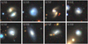 |
Fig. 1 Galaxy photometric image data from DESI DR9, demonstrating the issues of interfering galaxies around the target galaxy and galaxy blending in the photometric images. |
2.2 Image preprocessing
In order to address some issues present in the original photometric image provided by DESI, which is shown in Figure 1, we performed a series of preprocessing on the image. The preprocessing steps are shown in Figure 2, mainly including masking interfering galaxies, constraining the size of target galaxies, and target galaxy blending detection. The following sections will provide a detailed introduction to the existing issues and the steps to solve them.
2.2.1 Masking interfering galaxies
In this work, we focus on the target galaxy located at the center of the image, while we classify many other celestial objects in the image as interfering galaxies, as is shown in Figure 3a. To ensure the accuracy of the predicted results, we need to mask these interfering galaxies. We employed edge detection and contour fitting methods to mask the interfering galaxies, retaining only the target galaxy located at the center of the image.
Firstly, we converted the original color image to a grayscale image, as is depicted in Figure 3b. Subsequently, we calculated the initial threshold using Equation (1) for each image. We then preliminarily segmented the image into foreground and background regions based on this initial threshold, setting regions above the threshold as foreground (cobj) and regions below it as background (cbkg).
 (1)
(1)
where cmax and cmin represent the maximum and minimum grayscale values, respectively.
Then, we used Equation (2) to compute the average grayscale values for cobj and cbkg and updated the threshold accordingly.
 (2)
(2)
Next, we repeated this iterative process continuously until the optimal threshold was obtained when T_prev = T_next. Finally, based on the derived optimal threshold, we used image segmentation to set the pixel values of connected regions that are higher than this optimal threshold to 1, and the remaining pixel values to 0, thereby achieving image binarization, as is shown in Figure 3c.
After obtaining the binarized image, we adapted the edge detection method to extract the contours of each galaxy present in the image. Subsequently, we applied elliptical fitting to these galaxy contours, as is shown in Figure 3d. We used the distance between the center of the fit ellipse and the center of the image as an evaluation parameter, where celestial objects with smaller distances are closer to the center of the image. In this work, we have identified the celestial object with the smallest distance as the target galaxy. To ensure that the fit ellipse contains all the photometric information of the target galaxy, we enlarged the size of the ellipse by a ratio of 1:1.4. After fitting the ellipse successfully, we masked the regions outside the target galaxy with a black color, as is illustrated in Figure 3e.
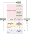 |
Fig. 2 Overall process of image preprocessing. |
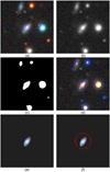 |
Fig. 3 Steps of image preprocessing. (a) The photometric image. (b) Converts the image to grayscale. (c) Binarizes the image, and (d) Obtains the contours of each galaxy in the image and performs elliptical fitting on these galaxies. (e) The target galaxy after covering the interfering galaxies. (f) The minimum circumcircle of the target galaxy. |
2.2.2 Constraining the size of the target galaxy
We obtained the Ztrue through spectral observation with a fiber diameter of 3 arcsec in SDSS. Therefore, when the size of the target galaxy is large, the optical fiber may not be able to fully capture the light of the entire galaxy, resulting in a Ztrue that may only represent localized information and potentially fail to reflect the overall characteristics of the galaxy. To ensure the accuracy of Ztrue, it is necessary to constrain the size of the region of interest corresponding to the target galaxy that will serve as an input to our DL model.
We used the method of minimum circumcircle (as is shown in Figure 3f) to constrain the size of the target galaxy. In this work, we plan to study galaxies with a radius within 6 arcsec, and the rationality and effectiveness of this choice are further explained in Section 4.3. Therefore, we constrained the radius of the minimum circumcircle of the target galaxy to approximately 23 pixels (each pixel in the DESI image corresponds to 0.262 arcsec, and 6 arcsec corresponds to about 23 pixels). We retained only those images with a circumcircle radius of the target galaxy between 0 and 6 arcsec for subsequent preprocessing tasks.
2.2.3 Target galaxy blending detection
Galaxy blending is a visual phenomenon. In astronomical observations, due to distance, perspective, or other factors, two or more galaxies can overlap or blend in the direction of the line of sight, especially in long-distance observations. This can cause their light to mix, making them appear as a single galaxy in images. This phenomenon makes it difficult for scientists to distinguish the characteristics of different galaxies, leading to some challenges in observing the structure, morphology, and measurement of some physical properties such as stellar mass and gas-phase metallicity. In the image dataset of DESI, we observe that many target galaxies exhibit galaxy blending, making it more complex to locate the target galaxy and predict the gasphase metallicity of it. Therefore, we need to perform galaxy blending detection to discard images where the target galaxies are blended. The results are shown in Figure 4. In this process, we employed the Photutils tool from the Astropy software package, which is primarily used for astronomical image analysis. The code used to address the blending issue is open-source. Next, we shall provide a detailed introduction to the steps of blending detection.
The target galaxy used in the blending detection process has already covered the interfering galaxies and its size has been constrained, thereby reducing the impact of background and background noise on the blending detection. We used the detect_source function from the Photutils tool to perform source detection on the target galaxy. To ensure the reliability of the detection, we set as criteria that the detected sources must have a minimum number of connected pixels (at least 10 pixels) and that each pixel value must exceed a specified threshold, which was set to 1.5 times the background root mean square.
If the target galaxy is a blended galaxy, its pixel values will be connected together during the detection process, forming a structure recognized as a single source. After obtaining the data source of the target galaxy located at the center point, we applied the deblend_source function from the Photutils tool. This function combines multi-threshold techniques and watershed segmentation to achieve source separation. If there is a “saddle point” between two celestial bodies, they are considered separate and can be deblended.
After that, we conducted source detection again. When the target galaxy exhibits blending, the number of detected sources after separation will exceed 1. In this case, we delete the image of the blended galaxy; conversely, if the number of detected sources after separation equals 1, we can conclude that the target galaxy is not blended, and we save that image. This blending detection process helps to maintain the quality of the dataset, ensuring the reliability and accuracy of subsequent predicted results.
After rigorous data selection and image preprocessing steps, we successfully constructed a dataset comprising 86 660 starforming galaxies with Ztrue. To ensure the reliability of model training and evaluation, we used uniform sampling based on the distribution of Ztrue of these 86 660 galaxies, ultimately selecting 25 000 samples. In Figure 5, we show the distribution of gas-phase metallicity (Z), stellar mass (M*), specific star formation rate (sSFR), and redshift (ɀ) for these 25 000 samples. We used the median gas-phase metallicity (oh_p50), median stellar mass (lgm_fib_p50), and median specific star formation rate (specfr_fib_p50) from the MPA-JHU DR8 catalog of SDSS to represent Z, M* , and sSFR, respectively. We randomly divided these 25 000 data into three parts in a ratio of 5:3:2: 50% for the training set, 30% for the validation set, and the remaining 20% as an independent test set. The distribution range of Ztrue in these three sets is generally consistent, as is shown in Figure 6. This partitioning strategy helps to effectively monitor and adjust the model during training process, while providing an objective evaluation of the model’s generalization performance. It is important to emphasize that the independent nature of the test set means we can only use the test set results for the final performance evaluation after completing all training steps.
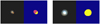 |
Fig. 4 Result of blending in the target galaxy and no blending in the target galaxy. |
3 Methodology
The main focus of this research is a regression problem. As a DL model, CNNs can effectively reduce the number of parameters and model complexity by automatically learning and capturing features of different scales and directions in images, demonstrating exceptional performance in regression tasks. However, when predicting the gas-phase metallicity (Z) of galaxies from their real photometric images, using traditional CNN models faces the following challenges:
(1) Failing to effective utilize the channel information: the gas distribution around galaxies is complex and diverse, and each channel of photometric galaxy images may contain key information related to Z . However, traditional CNN models mainly extract local features through convolution, and the handling of inter-channel dependencies is more implicit, which may result in some important information not being fully utilized. In the task of gas-phase metallicity prediction, the band information of each channel is crucial for accurate estimation. Failing to fully utilize this information can limit the model’s predictive performance. Therefore, itis necessary to design models that can better leverage information across different channels.
(2) Diversity in brightness and gas distribution: the photometric images of different galaxies can exhibit significant differences in brightness and gas distribution. For example, galaxies with higher brightness can show overly concentrated features due to image saturation, while galaxies with lower brightness can display less distinct features due to lower signal-to-noise ratios. Additionally, differences in gas distribution across galaxies can lead to an imbalance in feature learning, making it more difficult for the model to extract these features. These issues can limit the generalization ability of traditional CNN models on new data and increase the risk of overfitting.
To overcome these challenges, this paper proposes an effective method called GPM-ResNet1. To address issue (1), we introduced the efficient channel attention (ECA) module (Wang et al. 2020), which allows the model to better capture the dependencies between different channels in the photometric images, thereby fully utilizing the important information related to Z contained in each channel. To address issue (2), we employed the DropBlock regularization technique (Ghiasi et al. 2018), which helps the model learn more global features, enhancing its stability across samples with varying brightness and gas distributions, and effectively reducing the risk of overfitting. These improvements enable GPM-ResNet to demonstrate a satisfactory performance in the gas-phase metallicity prediction task. In the following sections, we shall provide a detailed description of the structure, working principles, and predictive performance of GPM-ResNet.
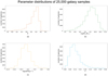 |
Fig. 5 Panels a, b, c, and d show the distributions of gas-phase metal- licity (Z), stellar mass (M*), specific star formation rate (sSFR), and redshift (ɀ), respectively, for the 25 000 samples used in this study. |
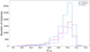 |
Fig. 6 Distribution of Ztrue on the training set, validation set, and test set, each consisting of 12 500, 7500, and 5000 samples, respectively. |
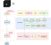 |
Fig. 7 Structure of the GPM-ResNet network. We input the preprocessed DESI photometric images into the model, where they sequentially pass through the multi-order feature extractor (ILO-Block and DHO-Block) and the parameter generator (PG-Block), ultimately obtaining the predicted values, Zpred. The definition of the ReLU activation function is f (x) = max(0, x). |
3.1 GPM-ResNet model
Figure 7 illustrates the network structure of GPM-ResNet, which mainly consists of two primary modules: the multi-order feature extractor and the parameter generator (PG-Block). The multiorder feature extractor is mainly composed of the ResNet-50 architecture (He et al. 2015), which is a deep residual network that can be used to effectively extract relevant features from photometric images. It consists of an initial low-order feature extractor (ILO-Block) and a deep high-order feature extractor (DHO-Block) that combines the ECA module and the DropBlock regularization technique. We initially processed the photometric image data with a size of 152 × 152 and Ztrue using ILO-Block. This module consists of a 7 × 7 convolution layer (Conv1), a batch normalization layer (BN), a ReLU activation function, and a 3 × 3 max pooling layer (MaxPool). The BN layer can accelerate the training speed of the model and improve its stability. In addition, the ReLU activation function, as one of the commonly used activation functions in DL, can enhance the expressive capability of the model. ILO-Block can preliminarily extract relevant low-order features from images. However, the gas features of galaxies are usually complex, so we designed a DHO-Block to extract higher-order features more effectively from these images.
The DHO-Block primarily adopts the Bottleneck structure of ResNet-50. It consists of four parts, each containing 3, 4, 6, and 3 Bottleneck blocks, respectively. Each Bottleneck block comprises three convolution layers in sequence: a 1 × 1 convolution layer, a 3 × 3 convolution layer, and another 1 × 1 convolution layer. The first 1 × 1 convolutional layer is used to reduce the number of channels in the input feature map, thereby reducing the computational and parameter complexity of the subsequent 3 × 3 convolutional layer. The middle 3 × 3 convolution layer is responsible for efficiently extracting relevant high-order features. The final 1 × 1 convolution layer not only restores the number of channels to their original dimensions, ensuring that the output feature map has the same number of channels as the input for subsequent processing, but also integrates the features extracted earlier, thereby enhancing the model’s expressive capability. This design allows GPM-ResNet to maintain efficient training and good performance, while effectively reducing computational complexity and improving prediction accuracy.
We introduced DropBlock regularization in the 3 × 3 convolution layer of each Bottleneck block. DropBlock is a regularization technique for CNN that reduces the risk of model overfitting and enhances its generalization capability in galaxies with different gas distributions and brightness variations. Furthermore, we integrated the ECA module into the second 1 × 1 convolution layer of each Bottleneck block. The ECA module can effectively capture channel dependencies in galaxy images, allowing the model to be more sensitive to the information related to Z across each channel, thereby enhancing feature extraction performance. Through the DHO-Block, we can extract deeper and more complex high-order features from the images, obtaining more accurate predicted results.
PG-Block includes a 7 × 7 average pooling layer (AvgPool), a ReLU activation function, and two linear layers: FC and New FC. Through the two linear layers, high-dimensional features are mapped to a one-dimensional output vector, whose outputs are the predicted values of gas-phase metallicity (Zpred). PG-Block effectively establishes the connection between the input photometric image and the output value Zpred, forming a complete prediction framework. The network architecture combines regularization techniques and a channel attention module, which enables GPM-ResNet to effectively learn the gas-phase metal- licity characteristics of galaxies, leading to a better performance.
3.2 Model training
In the context of solving regression problems, CNN uses a dataset with label values to calculate the error between the predicted outputs and the lable values, known as the loss function. This process involves gradient descent and backpropagation algorithms, which calculate the gradient of the loss function relative to the model parameters, thereby achieving parameter updates to minimize the loss function. In this work, we have chosen the mean squared error loss function, which can help the model make more accurate predictions.
During the training process, each epoch indicates that all training samples have undergone one forward propagation and a backward propagation process. To find the optimal combination of hyperparameters, we conducted the training for a long-term period of 50 epochs, passing photometric images to the model in batches of 256 samples per batch. Each batch utilizes gradient descent to adjust weight parameters. We used the Adam optimization algorithm (Kingma & Ba 2014) instead of the traditional stochastic gradient descent process to iteratively update the weights of the neural network through training data. We set the initial learning rate of the Adam optimizer to 0.01. After starting the training, we adjusted the learning rate every 10 epochs by reducing it to 10% of the original value, which is the current learning rate multiplied by 0.1. This setting allows for fast convergence in the early stages of training, while enabling finer adjustment of the model parameters in the later stages by reducing the learning rate, thereby improving the model’s final performance.
At the end of the training process, we obtain the loss function graph on the training set and validation set. By analyzing the loss function graph, we can evaluate whether the model exhibits overfitting or underfitting, and adjust the model hyperparameters or structure accordingly to achieve better performance and generalization ability. Finally, we evaluate the performance of the model based on the result of the test set.
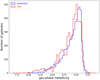 |
Fig. 8 Histogram illustrating the distribution of the gas-phase metal- licity in galaxies, with the blue line representing Zpred and the red line representing Ztrue. The bin widths for these two distributions are different. |
3.3 Comparing the true values and predicted values
The distribution of Ztrue and the predicted values Zpred obtained using GPM-ResNet is shown in Figure 8. We can observe from the graph that the distribution range of Zpred is slightly narrower than that of Ztrue, indicating that the model has errors in predicting extremely high or low values. To address these phenomena, it is necessary to further improve the model to enhance its applicability. Overall, the distribution of Zpred and Ztrue shows good consistency, verifying the robustness of the method.
Subsequently, we used the mean value (µ), standard deviation (σ), and normalized median absolute deviation (NMAD) as evaluation metrics to further analyze the prediction performance of GPM-ResNet, as is shown in Figure 9a. The NMAD is defined as:
 (3)
(3)
Among them, x represents the error set, which is the error between the predicted and the true values of each data point. The advantage of NMAD lies in its stronger robustness to outliers, enabling a more accurate reflection of data dispersion and providing a more stable and reliable measurement. The µ, σ, and NMAD for Zpred − Ztrue are 0.034 dex, 0.1181 dex, and 0.004 dex, respectively. From (a), we can observe that although GPM-ResNet exhibits some degree of overprediction in the low-metallicity region, the median line still maintains good consistency with the 1:1 line, indicating the model’s overall predictive reliability. The inset in the lower right corner shows the error distribution of ∆Z (Zpred − Ztrue), which approximately follows a normal distribution. However, due to the overprediction of the model on some data, ∆Z exhibits a heavy-tailed distribution trend near the positive residuals.
4 Model evaluation
In this section, we conduct a series of experiments to further evaluate the prediction performance of GPM-ResNet.
These experiments include: comparing the predictions obtained through the color–metallicity relation (Section 4.1); comparing the prediction performance of different network architectures on the same dataset (Section 4.2); examining the impact of different target galaxy sizes on the experimental results (Section 4.3); assessing the effects of different image resolutions and wavelength bands on the results (Sections 4.4 and 4.5); and exploring the MZR, while attempting to recover this relationship using the predicted values Zpred (Section 4.6). We shall now provide a detailed description of these experiments.
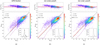 |
Fig. 9 (a) The Zpred obtained using GPM-ResNet. (b and c) The predicted results obtained from second-order and third-order polynomials fit based on the color-metallicity relation, respectively. In all three subplots, the top panel represents the residual density plot, where the solid red line represents y = 0 and the dashed purple line represents y = ±0.1dex. The bottom panel illustrates the density distribution: the solid black line indicates the 1:1 relationship; the solid red line represents the median line of Zpred, which varies with Ztrue; and the dashed purple line denotes the 1 σ scatter around the median. Each point represents a galaxy sample, and color coding highlights the kernel density estimation of galaxy density. |
4.1 Predicted results through the color–metallicity relation
In astronomical research, there exists a close relationship between the color of galaxies and their metallicity. Researchers regard color as an important observational parameter that can be used to infer the metallicity, temperature, and other properties of galaxies (Streich et al. 2014). A deeper investigation into the relationship between color and metallicity can help us better understand the processes of galaxy formation and evolution. Sanders et al. (2013) utilized star-forming galaxies from SDSS DR7 as research samples to explore the relationship between the color and gas-phase metallicity of these galaxies. In this paper, the author employed optical colors of star-forming galaxies, such as g – r, u – 𝑔, r – ɀ, and so on. The results indicated that incorporating color information can significantly enhance the accuracy of metallicity estimates for star-forming galaxies. Inspired by this research, in order to further explore the advantages of using DL method to predict gas-phase metallicity directly, we plan to analyze the color-metallicity relation in the DESI DR9 data used in this work, and obtain gas-phase metal- licity values based on this relationship. Subsequently, we shall compare the experimental results of the two methods.
In Section 2, we uniformly sampled 25 000 pieces of image data based on the distribution of Ztrue. In this section, we use these 25 000 samples to analyze the color–metallicity relation of the dataset and ultimately select image data from the test set to estimate gas-phase metallicity values based on this relationship. Firstly, we extracted the flux values in the 𝑔, r, and ɀ bands from the HDF5 files of the DESI Legacy Survey. Next, we calculated the corresponding magnitudes for the 𝑔, r, and ɀ bands using Equation (4) and further computed the magnitude differences for 𝑔 – r and r – ɀ.
 (4)
(4)
Finally, we analyzed the color-metallicity relation of these data using the optical colors 𝑔 – r and r – ɀ, as is shown in Figure 10. The figure shows a significant correlation between the gas-phase metallicity of galaxies and their color distribution: as the color difference increases, the metallicity gradually increases. Therefore, we plan to use the color–metallicity relation to estimate the gas-phase metallicity and compare the results with Zpred, which are directly predicted by GPM-ResNet.
In this study, we have used color values (𝑔 – r, r – ɀ) as the independent variables and Ztrue as the dependent variable, fitting second-order and third-order polynomials to describe their relationship, respectively. We used a sample of 5000 pieces of data from the test set in Section 2 and obtained the corresponding results based on the fit polynomials, which are named ZCMR2 and ZCMR3, respectively. The experimental results are shown in Figures 9b and 9c. Specifically, the σ for ZCMR2-Ztrue is 0.1562 dex, while the σ of ZCMR3-Ztrue is 0.1568 dex. The error values are quite similar, but the dispersion is greater for the third-order polynomial, which may be due to overfitting. This suggests that the second-order polynomial is sufficient for capturing the key information related to color.
However, compared to traditional methods based on the color–metallicity relationship, the predictions obtained using the GPM-ResNet model are better, with a σ of only 0.1181 dex, indicating a smaller error. Additionally, the µ and NMAD values obtained by the GPM-ResNet method are also significantly lower than those calculated through the color–metallicity relationship, further demonstrating its performance advantages. By observing Figure 9, we find that the scatter distribution in Figure 9a is more compact than that in Figures 9b and 9c. This improvement may be due to the ability of GPM-ResNet to leverage the intrinsic connection between galaxy morphology and metallicity, surpassing the limitations of relying solely on color information, and thus extracting more details. Specifically, GPM-ResNet not only effectively utilizes color information but also extracts additional information related to metallicity through morphological features in the images. By combining both color information and these additional features, the model significantly improves the prediction accuracy. A more detailed discussion of the relationship between galaxy morphology and metallicity can be found in Section 4.4.
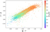 |
Fig. 10 Relation between color and metallicity in photometric images from DESI. The x and y axes represent colors 𝑔 − r and r − ɀ, respectively. Each data point corresponds to a galaxy, with its color code indicating the corresponding gas-phase metallicity value (oh_p50), which comes from the SDSS MPA-JHU DR8 catalog. |
4.2 Predicted results of other methods
In this section, we set out to validate the advantage of GPM- ResNet in estimating gas-phase metallicity through comparative analysis. Therefore, we selected four representative DL architectures: ResNet (He et al. 2015), MobileNet (Sandler et al. 2018), EfficientNet (Tan & Le 2019), and DenseNet (Huang et al. 2018), and trained them on the same dataset. We finally evaluated the performance of these models based on the test set, and we summarize the results in Table 1.
(1) ResNet is a classic deep neural network (DNN) architecture that introduces residual blocks. This design facilitates the training of deep networks and effectively addresses the issues of information decay and excessive amplification during the training process, thereby enabling the model to learn and capture complex features more stably.
(2) MobileNet adopts lightweight depthwise separable convolutions and linear bottleneck structures, significantly reducing the number of parameters and computational complexity of the model, while maintaining good feature extraction capabilities.
(3) EfficientNet further introduces width multipliers and depth multipliers on the basis of CNN architecture, and combines it with an inverted residual block structure, which can optimize and adapt the model structure through an automatic adjustment mechanism.
(4) DenseNet is known for its unique dense connectivity mechanism, ensuring that each layer is directly connected to all layers in front of it, maximizing parameter sharing and information flow.
According to the results in Table 1, GPM-ResNet outperforms other models in both the σ and NMAD metrics, demonstrating its stability and robustness in the predictions for the majority of samples. In particular, the NMAD metric, which is based on the median and absolute deviation, effectively reduces the influence of extreme values and provides a more accurate reflection of the prediction performance for most samples. However, GPM-ResNet shows a slightly inferior performance in the µ metric compared to other ResNet models. We speculate that this is primarily due to larger deviations when predicting extreme gas-phase metallicity values. Due to the small number and complex characteristics of extreme samples, the model is difficult to accurately learn their regularity, leading to larger prediction errors that subsequently impact the overall µ value.
In contrast, ResNet34 and ResNet101 perform better in the µ metric, which may be attributed to their relatively simple feature extraction methods, making them less sensitive to extreme samples and thereby reducing the impact of these samples on the overall mean error. However, this simplified feature extraction approach has limitations in capturing the complex features of the data, leading to poorer adaptability to galaxies with varying gas distributions and brightness, which explains their inferior performance in the σ and NMAD metrics. Additionally, MobileNet and EfficientNet have relatively weaker performance, which may be due to their network design not fully matching the characteristics of photometric image datasets. While they have optimized parameter count and computational efficiency, this may have reduced their ability to extract complex features, thus affecting their prediction accuracy. Moreover, although DenseNet has certain advantages in parameter sharing and information transmission, its high computational complexity can lead to overfitting during the training process, weakening its generalization ability on the test set and ultimately affecting its predictive performance.
Overall, GPM-ResNet effectively improves feature extraction capability and model robustness by incorporating the ECA mechanism and DropBlock regularization. GPM-ResNet outperforms other models in terms of the σ and NMAD metrics, demonstrating higher prediction accuracy for mainstream samples and a strong generalization ability for galaxies with varying gas distributions and brightness. Although it performs slightly worse than other ResNet models on the µ metric, this drawback is mainly attributed to deviations in extreme samples. Since extreme samples are relatively few, their impact on overall performance is limited. In the future, we plan to optimize the loss function design and improve training strategies to further enhance GPM-ResNet’s prediction accuracy on extreme samples, while reducing the risk of overfitting, thereby comprehensively improving the model’s overall performance.
Comparison of experiment results based on different methods.
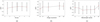 |
Fig. 11 (a–c) The predicted results for target galaxies of different sizes, different resolutions, and different wavelength bands of images, respectively. In these figures, the red circle in the center represents the µ, while the length of the error bars above and below the red circle corresponds to 1 σ. |
4.3 The impact of target galaxies of different sizes on the results
We obtained the label values’ Ztrue used in this article from the SDSS catalog; they are measured through a spectrograph with a diameter of 3 arcsec. When the target galaxy is relatively large, Ztrue may only represent partial regional information of the target galaxy. In this research, we performed preprocessing on the photometric images. We constrained the size of the target galaxies to within 6 arcsec using the method of the minimum circumcircle; however, this raises potential concerns regarding the accuracy of the label values.
To ensure the rationality of Ztrue, we estimated the gas-phase metallicity for target galaxies within different size ranges in this subsection. We divided the image data of the test set into five different intervals based on the radius of the minimum circumcircle of the target galaxy, as is illustrated in Figure 11a. By training the GPM-ResNet model on the image data for each interval, we evaluated the model’s performance in predicting gas-phase metallicity for galaxies of different sizes. The results indicate that as the size of the target galaxy increases, the σ gradually decreases and tends to stabilize. Compared to the results within the range of [3, 4] arcsec, the accuracy within the range of [5, 6] arcsec improved. This suggests that although the label values for larger galaxies may only cover local features, they can still represent information about the entire galaxy. Therefore, it is reasonable to set the minimum circumcircle radius of the target galaxy to within 6 arcsec. This choice effectively limits the size of the region of interest associated with the target galaxy, enabling GPM-ResNet to effectively capture the characteristics of gas-phase metallicity from the photometric images.
4.4 The impact of a different image resolution on the results
In this subsection, we investigate the impact of image resolution on the prediction performance of the model. This study will enhance our understanding of the importance of morphological features in images. We hypothesize that image resolution affects the prediction of gas-phase metallicity, such that as the resolution increases, the prediction error will gradually decrease. To verify this hypothesis, we employed bilinear interpolation to scale the resolution of the image data from the initial 152 × 152 to 16 × 16, 32 × 32, 64 × 64, and 128 × 128, and retrained the network. We present the results in Figure 11b. As was anticipated, the σ of the prediction error gradually decreases with increasing resolution, further supporting the significant role of morphological features in predicting gas-phase metallicity.
At lower resolutions, the gas-phase metallicity of galaxies is significantly underestimated. This underestimation primarily arises because resolution affects the details and amount of information presented in the images, which are crucial for understanding the physical properties of galaxies. Low-resolution images often lack the key information needed to predict gas properties, resulting in the model’s inability to capture important details, ultimately impacting the accuracy of predictions. Conversely, as the resolution increases from 32 × 32 to 64 × 64 and even higher, there is a significant improvement in model performance. This is because higher-resolution images provide richer content and more detailed morphological information, which helps to predict gas properties in galaxies more accurately.
The experiments in this subsection show that galaxy morphology contains rich information about the properties of galaxies, and the model can effectively learn gas properties from galaxy morphological features. Using the morphological features from photometric images can significantly improve the performance of GPM-ResNet. Among the different tested resolution combinations, the 152 × 152 resolution exhibits the smallest σ, further validating the rationality for selecting the 152 × 152 size of photometric images as input data.
4.5 The impact of different wavelength bands on the results
In addition to considering the impact of image resolution on predicted results, color information is also a crucial influencing factor. The photometric images in the DESI dataset consist of three bands: 𝑔, r, and ɀ, each carrying unique color information. Consequently, the selection of different bands may affect the predicted results. In this work, we use RGB images composed of three bands: 𝑔, r, and ɀ.
To evaluate the influence of different wavelength bands on the predicted results, we modified the original RGB images, while maintaining a fixed resolution of 152 × 152 pixels. We tested the prediction performance of single-band images (𝑔, r, ɀ), double-band images (𝑔r, 𝑔ɀ, rɀ), and three-band images (𝑔rɀ). Following the method outlined by Wu & Boada (2019), we replicated the data of the single-band images and put it into red, green, and blue channels accordingly. For the double-band images, such as the 𝑔r band, we copied the data from the 𝑔 band and r band into the blue and red channels, respectively, while the average value of these two bands were copied to the green channel. Subsequently, we trained the GPM-ResNet model on images from different bands, as is illustrated in Figure 11c.
The results indicate that the prediction performance of single-band images is relatively poor. However, introducing a second band leads to a significant enhancement in model performance, with the 𝑔ɀ band exhibiting the lowest prediction error. This improvement can be attributed to the fact that the 𝑔 band corresponds to wavelength in the blue light region, which can provide critical information about active young stars, enhancing the accuracy of gas-phase metallicity predictions. Furthermore, the ɀ band, which is typically situated in the longer-wavelength infrared region, can contain vital information regarding the elemental composition of galaxies, and its absence could adversely affect model performance. Overall, the combined use of the three bands (𝑔rɀ) provides the best prediction outcomes. This finding underscores the importance of color information in studying the properties of galaxies, demonstrating that the GPM-ResNet model can effectively leverage this color information to improve the estimation of metallicity. The diverse and rich information provided by different wavelength band images highlights the significance of utilizing multiband observational data for a comprehensive understanding of the composition and physical properties of galaxies.
4.6 The mass-metallicity relation
The correlation between stellar mass and gas-phase metallic- ity in galaxies is commonly referred to as the mass–metallicity relation (MZR) (e.g., Lequeux et al. 1979; Tremonti et al. 2004). Exploring this relationship enhances our understanding of galaxy formation and evolution. The MZR is believed to form through the interaction of various processes, including gas inflow, outflow of metal-rich gas, and star formation (Larson 1974; Garnett 2002; Tremonti et al. 2004; Dalcanton et al. 2004; Ellison et al. 2008). This relationship reveals a strong association between a galaxy’s stellar mass and its chemical element abundance: the larger the mass of the galaxy, the higher the metallicity of its gas. Within the stellar mass range of 8.5 < log(M*/M⊙) < 11.5, the scatter distribution of the true metallic- ity (Ztrue) exhibits a characteristic of approximately σ ≈ 0.10dex (Tremonti et al. 2004). Furthermore, this relationship can be well fit by a polynomial, with the specific expression as follows:
![Mathematical equation: $\matrix{ {12 + \log ({\rm{O}}/{\rm{H}}) = - 1.492 + 1.847\log \left( {{{\rm{M}}_ * }/{{\rm{M}}_ \odot }} \right)} \cr {\,\,\,\,\,\,\,\,\,\,\,\,\,\,\,\,\,\,\,\,\,\,\,\,\,\,\,\,\,\,\,\, - 0.08026{{\left[ {\log \left( {{{\rm{M}}_ * }/{{\rm{M}}_ \odot }} \right)} \right]}^2}.} \cr } $](/articles/aa/full_html/2025/02/aa52813-24/aa52813-24-eq5.png) (5)
(5)
Equation (5) is effective within the range of 8.5 < log(M*/M⊙) < 11.5, where log(M*/M⊙) represents the value of stellar mass.
4.6.1 Predicting the gas-phase metallicity through stellar mass
We knew there is a close relationship between stellar mass and gas-phase metallicity; thus, we considered using Equation (5) to estimate the values of gas-phase metallicity. Firstly, we trained the method to obtain the mass from photometric images, then utilized Equation (5) to convert these mass values into gas-phase metallicity values. For this purpose, we used GPM-ResNet to predict stellar mass. It is worth noting that star mass prediction methods based on neural networks have gained widespread application in recent years. For example, Alfonzo et al. (2024), Wu & Boada (2019), and Zhong et al. (2024) successfully predicted stellar mass using CNNs, while Surana et al. (2020) employed DNNs to accomplish similar tasks. These works provide important references and inspirations for our research. After the image preprocessing steps outlined in Section 2, we obtained 86 660 star-forming galaxies. In this section, we crossmatch this data with the stellar mass values (lgm_fib_p50) from the SDSS MPA-JHU DR8 catalog, which are referred to as M* (true) in this paper. To ensure the quality of the data, we removed invalid values of mass (lgm_fib_p50 = −9999), ultimately retaining 85 979 valid pieces of data.
Next, we uniformly sampled 25000 pieces of image data based on the distribution of lgm_fib_p50 and divided them into training, validation, and testing sets in a ratio of 5:3:2. We re-ran the model and evaluated the predictions based on 5000 test samples, with the results referred to as M*(pred) in this study. As is shown in Figure 12a, the µ of the difference M*(pred) − M*(true) is 0.098 dex, the σ is 0.3583 dex, and the NMAD is 0.0151 dex. The median line is also consistent with the 1:1 line, indicating that this method can predict stellar masses from photometric images with relatively high accuracy.
Considering the applicable range of Equation (5), we selected data with M* (true) values between 8.5 and 11.5 from the test set, resulting in 4840 samples. We then used Equation (5) to convert the predicted mass values of these data into gas-phase metallicity values and refer to them as ZMZR, with the results illustrated in Figure 12b. The µ, σ, and NMAD of ZMZR − Ztrue are −0.09 dex, 0.1208 dex, and 0.0045 dex, respectively. We observe that the scatter distribution in Figure 9a is more compact compared to the results in Figure 12b, with smaller values for both σ and NMAD. This finding suggests that the GPM- ResNet method can directly predict gas-phase metallicity from photometric images in a more powerful way, omitting the step of conversion through Equation (5), further verifying the efficiency and accuracy of this DL method.
4.6.2 Recovering the mass–metallicity relation through GPM-ResNet
Tremonti et al. (2004) conducted a detailed exploration of the MZR and presented a corresponding relationship plot. To further evaluate the performance of GPM-ResNet, we attempt to recover this relation using the predicted gas-phase metallicity values (Zpred). In Figure 13, we plot the relationship between Zpred and the true stellar mass values M*(true). To assess the effectiveness of the recovery, the figure also displays the median relation of the MZR along with the ±1σ scatter (approximately 0.10 dex) proposed by Tremonti et al. (2004).
We observe from the figure that the MZR follows a distinct linear trend within a certain range and gradually flattens at higher mass ranges. Despite some minor discrepancies, the median line of Zpred (solid red line) maintains a consistent trend with the median relation of the MZR (solid black line). Furthermore, the 1σ scatter of Zpred (dashed red line) shows a similar trend to the 1σ scatter of the empirical MZR (dashed black line).
GPM-ResNet exhibits some errors when predicting extremely high or low gas-phase metallicity values, leading to small deviations in recovering the MZR relation. However, the overall results remain consistent with the empirical MZR. This indicates that Zpred can successfully recover the MZR. These findings further highlight the superiority of GPM-ResNet in predicting gas-phase metallicity and validate its potential applications in galaxy physics research.
5 Applications
In the previous section, we proposed a method called GPM- ResNet, which aims to predict the gas-phase metallicity of galaxies from the photometric images. We evaluated the performance of this method in Section 4, further demonstrating its superiority in predicting gas-phase metallicity. In this section, we apply the GPM-ResNet method to predict the gasphase metallicity of spiral galaxies (EXP) from the DESI DR9 image dataset and combine other known properties of EXP to construct a comprehensive catalog. The following sections will provide a detailed description of these processes.
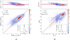 |
Fig. 12 (a) The results of estimating stellar mass using the GPM-ResNet method. (b) The derived gas-phase metallicity values based on the MZR. The top panel of both subplots displays the residual density plot, where the solid red line represents y = 0 and the dashed purple line represents y = ±0.1dex. The bottom panel is a density plot, with solid black lines indicating a 1:1 relationship; the solid red line represents the median line of the predicted values, and the dashed purple line represents 1 σ scatter around the median. The meanings of these lines are consistent with the corresponding lines in Figure 9. The color coding in the figures emphasizes the core density estimation of the galaxies. |
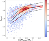 |
Fig. 13 MZR recovered through Zpred. The solid red line represents the median of Zpred, while the dashed red line indicates the ±1σ range relative to the median line. The solid black line shows the median relation of the MZR proposed by Tremonti et al. (2004), and the dashed black line represents the ±1σ range, which is 0.1 dex from this median line. These lines clearly illustrate the relationship between the MZR recovered from Zpred and the empirical MZR. |
5.1 Spiral galaxies (EXP)
The official website of the DESI DR9 dataset2 states that the DR9 dataset includes six morphological types, five of which are used in the Tractor fitting procedure. These morphological types include point sources (“PSF”), exponential galaxies with a variable radius (“REX”), elliptical galaxies (“DEV”), spiral galaxies (“EXP”), and Sersic profiles (“SER”). The sixth morphological type is “DUP,” which is specifically designated for Gaia sources.
Among these six morphological types, spiral galaxies (EXP) are a significant category. They are renowned for their distinctive spiral structure, typically appearing in a spiral pattern composed of bright arm-like structures and dark dust lanes. These structures rotate around the center of the galaxy, giving the entire system a prominent spiral appearance. Spiral galaxies are generally rich in gas, dust, young stars, and interstellar matter, often exhibiting blue hues, making them become a primary focus of astronomical research (e.g., Springel & Hernquist 2005; Sánchez-Menguiano et al. 2019; Frosst et al. 2022; Wei et al. 2024). Based on these studies, we have learned that spiral galaxies accumulate abundant gas, which is considered an important raw material for star formation. Consequently, we hypothesize that there may be more active star formation activity in spiral galaxies (EXP). The abundant gas content and active star formation activity in spiral galaxies typically provide more rich information about gas-phase metallicity. Therefore, we plan to use the GPM-ResNet method to predict the gas-phase metallic- ity of EXP in the DR9 dataset. Through this research, we hope to further understand the characteristics of spiral galaxies and the processes of element formation and evolution in the universe.
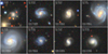 |
Fig. 14 Examples of photometric images of spiral galaxies (EXP) in the DESI DR9 dataset. |
Catalog of spiral galaxies (EXP) in DESI DR9.
5.2 Catalog of spiral (EXP) galaxies in DESI DR9
Figure 14 shows the photometric image data of EXP from the DESI DR9 dataset. In this section, we estimate the gas-phase metallicity of the EXP galaxies using the GPM-ResNet method. Firstly, we obtained 8 462 944 EXP galaxies by selecting data in the HDF5 files from the DESI Legacy Survey3 (source_type = b’EXP’). Next, we preprocessed these photometric images using the method described in Section 2.2, and ultimately constructed a photometric image dataset containing 5 095 815 EXP galaxies.
We then used GPM-ResNet to predict the gas-phase metallic- ity (Z_pred) of all EXP galaxies in this dataset and integrated the prediction results with other known properties of the EXP galaxies into a table. Known properties include the right ascension (ra), the declination (dec), camera and filter settings (release), the brick sky position (brickid), the catalog object number within the brick (objid), the photometric redshift (z_phot_median), and the apparent magnitude in the r band (mag_r), which were obtained through HDF5 files from DESI Legacy Survey and crossmatching with the SDSS MPA-JHU DR8 catalog. We provide further details in Table 2, which lists some sample entries. Additionally, we analyzed the distributions of z_phot_median, mag_r, and Z_pred, as is shown in Figure 15. In this dataset, the median value of z_phot_median is 0.31, the median of mag_r is 20.25, and the median of Z_pred is 8.82.
In Figure 16, we compare the distribution of gas-phase metal- licity for EXP galaxies with that of 86 660 star-forming galaxies. The gas-phase metallicity of EXP galaxies is predicted using the GPM-ResNet model, while the gas-phase metallicity of starforming galaxies is obtained from the SDSS MPA-JHU DR8 catalog. The results show that the median gas-phase metallicity of EXP galaxies is 8.82, whereas the median for star-forming galaxies is 8.95. We can observe from the graph that starforming galaxies generally have higher gas-phase metallicity than EXP galaxies. This difference may stem from variations in morphological and spectral categories. To further explore the reasons behind this discrepancy, we plan to analyze the correlation between morphological and spectral types. These subsequent studies will contribute to a deeper understanding of the characteristics of different categories of galaxies and their impact on gas-phase metallicity.
 |
Fig. 15 Panels a, b, and c show the distributions of the photometric redshift (z_phot_median), apparent magnitude in the r band (mag_r), and gas-phase metallicity (Z_pred) for EXP galaxies in DESI DR9 dataset. The plot displays the y-axis in scientific notation. Among them, the values of Z_pred are predicted using the GPM-ResNet method proposed in this paper. |
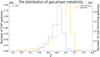 |
Fig. 16 Comparison of the gas-phase metallicity distribution between EXP galaxies and star-forming galaxies in the DESI DR9 dataset. The blue curve represents the distribution of EXP galaxies, with the gasphase metallicity values (Z_pred) predicted using the GPM-ResNet model; while the yellow curve shows the distribution of star-forming galaxies, with their gas-phase metallicity values (oh_p50) obtained from the SDSS MPA-JHU DR8 catalog. The left y-axis displays the number of EXP galaxies, while the right y-axis shows the number of starforming galaxies. Both y axes are presented in scientific notation. |
6 Conclusions
In this study, we have conducted an in-depth discussion about the gas-phase metallicity of galaxies. Our research is novel as (1) we have combined data from two different survey projects, SDSS and DESI; (2) we have proposed a method called GPM-ResNet to predict the gas-phase metallicity of galaxies by training on three-band photometric images (𝑔, r, ɀ) with a resolution of 152x152 from the DESI DR9 dataset; and (3) we have applied GPM-ResNet to spiral galaxies (EXP).
In order to enhance the prediction accuracy, we crossmatched the image data from DESI DR9 with the true gas-phase metallic- ity values (Ztrue) measured in the SDSS MPA-JHU DR8 catalog before the experiment, using Ztrue as the label data for this study. Ultimately, we obtained 86 660 pieces of image data on star-forming galaxies. Subsequently, in order to provide a cleaner dataset for subsequent experiments, we employed a comprehensive preprocessing approach on the photometric images, which included masking interfering galaxies, constraining the size of target galaxies, and detecting galaxy blending. GPM-ResNet utilizes real photometric images for predictions, significantly improving efficiency and extending the observable range, particularly for galaxies where spectral information is challenging to obtain. We trained GPM-ResNet and validated its performance by evaluating the residuals between the predicted values (Zpred) and the true values (Ztrue). The µ, σ, and NMAD for Zpred − Ztrue are 0.034 dex, 0.1181 dex, and 0.004 dex, respectively, indicating that GPM-ResNet possesses strong feature extraction capabilities in predicting gas-phase metallicity and highlighting its advantages in making predictions from photometric images.
Next, in order to further validate the superiority of GPM- ResNet, we conducted a series of experiments to evaluate the model performance, mainly including the following aspects:
(1) Discussion of the color–metallicity relation: we fit second-order and third-order polynomials to describe the relationship between color and metallicity. Through the fit polynomials, we obtained the predicted results for the gas-phase metallicity, with σ of 0.1562 dex and 0.1568 dex, respectively. After comparing the results with the predicted result of GPM- ResNet, we find that the latter has a smaller σ, indicating that GPM-ResNet has significant advantages in predicting gas-phase metallicity from photometric images.
(2) Comparison of different network architectures: based on the same dataset, we compared the predicted results of GPM-ResNet with those of four other network models (ResNet, MobileNet, EfficientNet, and DenseNet). The results show that GPM-ResNet achieves lower σ and NMAD values compared to other network models, indicating its smaller prediction errors for the majority of samples and higher stability. However, due to larger deviations when predicting extreme gas-phase metallicity values (e.g., very high or very low), the µ of GPM-ResNet is slightly higher than that of other ResNet models.
(3) Prediction performance across different galaxy sizes: we discussed the prediction performance of GPM-ResNet for target galaxies of different sizes and found that the model can provide relatively stable and accurate predictions for target galaxies of various sizes.
(4) Analysis of the impact of galaxy morphology and color information: by training photometric images with different resolutions (fixed wavelength bands) and different wavelength bands (fixed resolution), we found that as the resolution and wavelength bands increases, the prediction error shows a decreasing trend.
The morphological characteristics and color information of galaxies contain rich information related to gas-phase metal- licity, which is of great significance in predicting the physical properties of galaxies.
We further discussed the MZR. We used the GPM-ResNet to predict stellar mass and converted the predicted results to the corresponding gas-phase metallicity using Equation (5). Through comparing these converted results with Zpred, we note that GPM- ResNet’s predictions exhibit a tighter scatter distribution and smallererrors. Moreover, through utilizing Zpred, we successfully restored the MZR. Although there are some minor deviations from the empirical MZR, the overall trend is consistent, further validating the superior performance of GPM-ResNet. This study also enhances our understanding of the relationship between stellar mass and metallicity.
Finally, we used GPM-ResNet to predict the gas-phase metallicity of spiral galaxies (EXP) in the DESI DR9 dataset, with the predicted values referred to as Z_pred. We combined these predictions with other known properties of EXP galaxies to construct a comprehensive catalog of EXP galaxies. In this paper, we have analyzed the distribution of the photometric redshift (z_phot_median), r-band apparent magnitude (mag_r), and gas-phase metallicity (Z_pred) of the EXP galaxies to gain a deeper understanding of their physical properties and evolutionary processes. Additionally, we compared the gas-phase metallicity distribution of EXP galaxies with that of star-forming galaxies used for training the GPM-ResNet model. The gasphase metallicity values (oh_p50) for star-forming galaxies were derived from the SDSS MPA–JHU DR8 catalog. The results show that the gas-phase metallicity values of star-forming galaxies are generally higher than those of EXP galaxies.
In future research, we plan to expand the data range of our study and further optimize and improve GPM-ResNet to address potential errors in predicting extremely high or low gas-phase metallicity values, enhancing the robustness of the method. We also plan to explore and explain the reasons for the deviation in gas-phase metallicity values between EXP galaxies and starforming galaxies. These investigations are expected to provide new perspectives for future astronomical research and promote a deeper understanding of galaxy evolution and cosmic structure.
Data availability
Table 2 is available in electronic form at the CDS via anonymous ftp to cdsarc.cds.unistra.fr (130.79.128.5) or via https://cdsarc.cds.unistra.fr/viz-bin/cat/J/A+A/694/A271.
Acknowledgements
The work is supported by the National Natural Science Foundation of China (Grant Nos. 12473105, 12473106, 62272336, 12273075), Projects of Science and Technology Cooperation and Exchange of Shanxi Province (Grant Nos. 202204041101037, 202204041101033), The central government guides local funds for science and technology development (YDZJSX2024D049), the science research grant from the China Manned Space Project with No. CMS-CSST-2021- B03, and Guanghe Fund (No. ghfund202407027490).
References
- Ackermann, S., Schawinski, K., Zhang, C., Weigel, A. K., & Turp, M. D. 2018, MNRAS, 479, 415 [NASA ADS] [CrossRef] [Google Scholar]
- Alfonzo, J. P., Iyer, K. G., Akiyama, M., et al. 2024, ApJ, 967, 152 [NASA ADS] [CrossRef] [Google Scholar]
- Bai, Y., Liu, J., Wang, S., & Yang, F. 2019, AJ, 157, 9 [Google Scholar]
- Baqui, P. O., Marra, V., Casarini, L., et al. 2021, A&A, 645, A87 [EDP Sciences] [Google Scholar]
- Belli, S., Jones, T., Ellis, R. S., & Richard, J. 2013, ApJ, 772, 141 [NASA ADS] [CrossRef] [Google Scholar]
- Blanc, G. A., Lu, Y., Benson, A., Katsianis, A., & Barraza, M. 2019, ApJ, 877, 6 [NASA ADS] [CrossRef] [Google Scholar]
- Bonjean, V., Aghanim, N., Salomé, P., et al. 2019, A&A, 622, A137 [NASA ADS] [CrossRef] [EDP Sciences] [Google Scholar]
- Bottrell, C., Hani, M. H., Teimoorinia, H., et al. 2019, MNRAS, 490, 5390 [NASA ADS] [CrossRef] [Google Scholar]
- Brinchmann, J., Charlot, S., White, S. D. M., et al. 2004, MNRAS, 351, 1151 [Google Scholar]
- Buck, T., & Wolf, S. 2021, arXiv e-prints [arXiv:2111.01154] [Google Scholar]
- Cai, J., Yan, Z., Yang, H., et al. 2024, A&A, 687, A15 [NASA ADS] [CrossRef] [EDP Sciences] [Google Scholar]
- Cheng, T.-Y., Li, N., Conselice, C. J., et al. 2020, MNRAS, 494, 3750 [NASA ADS] [CrossRef] [Google Scholar]
- Cheng, T.-Y., Conselice, C. J., Aragón-Salamanca, A., et al. 2021, MNRAS, 507, 4425 [NASA ADS] [CrossRef] [Google Scholar]
- Chu, J., Tang, H., Xu, D., Lu, S., & Long, R. 2024, MNRAS, 528, 6354 [NASA ADS] [CrossRef] [Google Scholar]
- Cullen, F., Cirasuolo, M., McLure, R. J., Dunlop, J. S., & Bowler, R. A. A. 2014, MNRAS, 440, 2300 [NASA ADS] [CrossRef] [Google Scholar]
- Curti, M., Mannucci, F., Cresci, G., & Maiolino, R. 2020, MNRAS, 491, 944 [Google Scholar]
- Dalcanton, J. J., Yoachim, P., & Bernstein, R. A. 2004, ApJ, 608, 189 [NASA ADS] [CrossRef] [Google Scholar]
- Dey, A., Schlegel, D. J., Lang, D., et al. 2019, AJ, 157, 168 [Google Scholar]
- Dieleman, S., Willett, K. W., & Dambre, J. 2015, MNRAS, 450, 1441 [NASA ADS] [CrossRef] [Google Scholar]
- D’Isanto, A., & Polsterer, K. L. 2018, A&A, 609, A111 [Google Scholar]
- Doorenbos, L., Sextl, E., Heng, K., et al. 2024, arXiv e-prints [arXiv:2406.18175] [Google Scholar]
- Du, M., Ho, L. C., Debattista, V. P., et al. 2020, ApJ, 895, 139 [CrossRef] [Google Scholar]
- Ellison, S. L., Patton, D. R., Simard, L., & McConnachie, A. W. 2008, ApJ, 672, L107 [NASA ADS] [CrossRef] [Google Scholar]
- Euclid Collaboration (Bisigello, L., et al.) 2023, MNRAS, 520, 3529 [NASA ADS] [CrossRef] [Google Scholar]
- Fabbro, S., Venn, K. A., O’Briain, T., et al. 2018, MNRAS, 475, 2978 [Google Scholar]
- Fang, G., Ba, S., Gu, Y., et al. 2023, AJ, 165, 35 [NASA ADS] [CrossRef] [Google Scholar]
- Ferreira, L., Conselice, C. J., Duncan, K., et al. 2020, ApJ, 895, 115 [NASA ADS] [CrossRef] [Google Scholar]
- Frosst, M., Courteau, S., Arora, N., et al. 2022, MNRAS, 514, 3510 [NASA ADS] [CrossRef] [Google Scholar]
- Gao, Y., Bao, M., Yuan, Q., et al. 2018, ApJ, 869, 15 [NASA ADS] [CrossRef] [Google Scholar]
- Garnett, D. R. 2002, ApJ, 581, 1019 [NASA ADS] [CrossRef] [Google Scholar]
- Ghiasi, G., Lin, T.-Y., & Le, Q. V. 2018, arXiv e-prints [arXiv:1810.12890] [Google Scholar]
- Haurberg, N. C., Salzer, J. J., Cannon, J. M., & Marshall, M. V. 2015, ApJ, 800, 121 [NASA ADS] [CrossRef] [Google Scholar]
- He, K., Zhang, X., Ren, S., & Sun, J. 2015, arXiv e-prints [arXiv:1512.03385] [Google Scholar]
- Hefele, J. D., Bortolussi, F., & Portegies Zwart, S. 2020, A&A, 634, A45 [NASA ADS] [CrossRef] [EDP Sciences] [Google Scholar]
- Henghes, B., Thiyagalingam, J., Pettitt, C., Hey, T., & Lahav, O. 2022, MNRAS, 512, 1696 [NASA ADS] [CrossRef] [Google Scholar]
- Hernández, C. A., González, R. E., & Padilla, N. D. 2023, MNRAS, 524, 4653 [CrossRef] [Google Scholar]
- Hezaveh, Y. D., Perreault Levasseur, L., & Marshall, P. J. 2017, Nature, 548, 555 [Google Scholar]
- Hocking, A., Geach, J. E., Sun, Y., & Davey, N. 2018, MNRAS, 473, 1108 [CrossRef] [Google Scholar]
- Hoyle, B. 2016, Astron. Comput., 16, 34 [NASA ADS] [CrossRef] [Google Scholar]
- Huang, G., Liu, Z., van der Maaten, L., & Weinberger, K. Q. 2018, arXiv e-prints [arXiv:1608.06993] [Google Scholar]
- Hunt, L. J., Pimbblet, K. A., & Benoit, D. M. 2024, MNRAS, 529, 479 [CrossRef] [Google Scholar]
- Ivezić, Ž., Kahn, S. M., Tyson, J. A., et al. 2019, ApJ, 873, 111 [Google Scholar]
- Jeffrey, N., Lanusse, F., Lahav, O., & Starck, J.-L. 2020, MNRAS, 492, 5023 [Google Scholar]
- Kacprzak, G. G., van de Voort, F., Glazebrook, K., et al. 2016, ApJ, 826, L11 [CrossRef] [Google Scholar]
- Kauffmann, G., Heckman, T. M., White, S. D. M., et al. 2003, MNRAS, 341, 33 [Google Scholar]
- Kewley, L. J., & Ellison, S. L. 2008, ApJ, 681, 1183 [Google Scholar]
- Kim, E. J., & Brunner, R. J. 2016, MNRAS, 464, 4463 [Google Scholar]
- Kingma, D. P., & Ba, J. 2014, arXiv e-prints [arXiv:1412.6980] [Google Scholar]
- Kobulnicky, H. A., & Kewley, L. J. 2004, ApJ, 617, 240 [CrossRef] [Google Scholar]
- Langeroodi, D., Hjorth, J., Chen, W., et al. 2023, ApJ, 957, 39 [NASA ADS] [CrossRef] [Google Scholar]
- Lanusse, F., Ma, Q., Li, N., et al. 2018, MNRAS, 473, 3895 [Google Scholar]
- Larson, R. B. 1974, MNRAS, 169, 229 [NASA ADS] [CrossRef] [Google Scholar]
- Laureijs, R., Amiaux, J., Arduini, S., et al. 2011, arXiv e-prints [arXiv:1110.3193] [Google Scholar]
- Lee, H., Skillman, E. D., Cannon, J. M., et al. 2006, ApJ, 647, 970 [NASA ADS] [CrossRef] [Google Scholar]
- Lequeux, J., Peimbert, M., Rayo, J. F., Serrano, A., & Torres-Peimbert, S. 1979, A&A, 80, 155 [Google Scholar]
- Li, C., Zhang, Y., Cui, C., et al. 2022a, MNRAS, 518, 513 [CrossRef] [Google Scholar]
- Li, J., Tu, L., Gao, X., et al. 2022b, MNRAS, 517, 808 [NASA ADS] [CrossRef] [Google Scholar]
- Lian, J. H., Li, J. R., Yan, W., & Kong, X. 2015, MNRAS, 446, 1449 [NASA ADS] [CrossRef] [Google Scholar]
- Looser, T. J., D’Eugenio, F., Piotrowska, J. M., et al. 2024, MNRAS, 532, 2832 [NASA ADS] [CrossRef] [Google Scholar]
- Luo, A.-L., Zhao, Y.-H., hao, G., et al. 2015, Res. Astron. Astrophys., 15, 1095 [Google Scholar]
- Ma, X., Hopkins, P. F., Faucher-Giguère, C.-A., et al. 2016, MNRAS, 456, 2140 [NASA ADS] [CrossRef] [Google Scholar]
- Mannucci, F., Cresci, G., Maiolino, R., Marconi, A., & Gnerucci, A. 2010, MNRAS, 408, 2115 [NASA ADS] [CrossRef] [Google Scholar]
- Marino, R. A., Rosales-Ortega, F. F., Sánchez, S. F., et al. 2013, A&A, 559, A114 [NASA ADS] [CrossRef] [EDP Sciences] [Google Scholar]
- Martin, G., Kaviraj, S., Hocking, A., Read, S. C., & Geach, J. E. 2020, MNRAS, 491, 1408 [Google Scholar]
- Muyskens, A. L., Goumiri, I. R., Priest, B. W., et al. 2022, AJ, 163, 148 [NASA ADS] [CrossRef] [Google Scholar]
- Obreja, A., Macciò, A. V., Moster, B., et al. 2018, MNRAS, 477, 4915 [NASA ADS] [CrossRef] [Google Scholar]
- Obreja, A., Dutton, A. A., Macciò, A. V., et al. 2019, MNRAS, 487, 4424 [NASA ADS] [CrossRef] [Google Scholar]
- Omori, K. C., Bottrell, C., Walmsley, M., et al. 2023, A&A, 679, A142 [NASA ADS] [CrossRef] [EDP Sciences] [Google Scholar]
- Pasquet, J., Bertin, E., Treyer, M., Arnouts, S., & Fouchez, D. 2019, A&A, 621, A26 [NASA ADS] [CrossRef] [EDP Sciences] [Google Scholar]
- Petrillo, C. E., Tortora, C., Chatterjee, S., et al. 2017, MNRAS, 472, 1129 [Google Scholar]
- Petrillo, C. E., Tortora, C., Vernardos, G., et al. 2019, MNRAS, 484, 3879 [Google Scholar]
- Pöntinen, M., Granvik, M., Nucita, A. A., et al. 2023, A&A, 679, A135 [NASA ADS] [CrossRef] [EDP Sciences] [Google Scholar]
- Posses, A. C., Aravena, M., González-López, J., et al. 2023, A&A, 669, A46 [NASA ADS] [CrossRef] [EDP Sciences] [Google Scholar]
- Sánchez-Menguiano, L., Sánchez Almeida, J., Muñoz-Tuñón, C., et al. 2019, ApJ, 882, 9 [CrossRef] [Google Scholar]
- Sánchez-Menguiano, L., Sánchez, S. F., Sánchez Almeida, J., & Muñoz-Tuñón, C. 2024, A&A, 682, L11 [NASA ADS] [CrossRef] [EDP Sciences] [Google Scholar]
- Sanders, N. E., Levesque, E. M., & Soderberg, A. M. 2013, ApJ, 775, 125 [Google Scholar]
- Sandler, M., Howard, A., Zhu, M., Zhmoginov, A., & Chen, L.-C. 2018, arXiv e-prints [arXiv:1801.04381] [Google Scholar]
- Sanders, R. L., Shapley, A. E., Jones, T., et al. 2021, ApJ, 914, 19 [CrossRef] [Google Scholar]
- Shen, J., & Zheng, X.-W. 2020, Res. Astron. Astrophys., 20, 159 [CrossRef] [Google Scholar]
- Smirnov, E. A., & Markov, A. B. 2017, MNRAS, 469, 2024 [NASA ADS] [CrossRef] [Google Scholar]
- Springel, V., & Hernquist, L. 2005, ApJ, 622, L9 [Google Scholar]
- Streich, D., de Jong, R. S., Bailin, J., et al. 2014, A&A, 563, A5 [NASA ADS] [CrossRef] [EDP Sciences] [Google Scholar]
- Surana, S., Wadadekar, Y., Bait, O., & Bhosale, H. 2020, MNRAS, 493, 4808 [NASA ADS] [CrossRef] [Google Scholar]
- Tan, M., & Le, Q. V. 2019, arXiv e-prints [arXiv:1905.11946] [Google Scholar]
- Tremonti, C. A., Heckman, T. M., Kauffmann, G., et al. 2004, ApJ, 613, 898 [Google Scholar]
- Walmsley, M., Lintott, C., Géron, T., et al. 2022, MNRAS, 509, 3966 [Google Scholar]
- Wang, E., & Lilly, S. J. 2021, ApJ, 910, 137 [NASA ADS] [CrossRef] [Google Scholar]
- Wang, Q., Wu, B., Zhu, P., et al. 2020, arXiv e-prints [arXiv:1910.03151] [Google Scholar]
- Wang, L.-L., Yang, G.-J., Zhang, J.-L., et al. 2024, MNRAS, 527, 10557 [Google Scholar]
- Wei, J., Xu, Y., Lin, Z., et al. 2024, arXiv e-prints [arXiv:2410.07676] [Google Scholar]
- Wu, J. F., & Boada, S. 2019, MNRAS, 484, 4683 [NASA ADS] [CrossRef] [Google Scholar]
- Wu, J. F., & Peek, J. E. G. 2020, arXiv e-prints [arXiv:2009.12318] [Google Scholar]
- Yang, H., Zhou, L., Cai, J., et al. 2023, MNRAS, 518, 5904 [Google Scholar]
- Yang, H.-F., Wang, R., Cai, J.-H., et al. 2024, ApJS, 272, 43 [NASA ADS] [CrossRef] [Google Scholar]
- York, D. G., Adelman, J., Anderson, John E., J., et al. 2000, AJ, 120, 1579 [NASA ADS] [CrossRef] [Google Scholar]
- Zhong, J., Deng, Z., Li, X., et al. 2024, MNRAS, 531, 2011 [CrossRef] [Google Scholar]
The complete code and pre-trained models can be publicly obtained at: https://github.com/tian-mark/parameter-measurement
The official website of the DESI DR9 dataset: https://www.legacysurvey.org/dr9/description/
The official repository of the DESI Legacy Survey is available at: https://github.com/georgestein/ssl-legacysurvey
All Tables
All Figures
|
Fig. 1 Galaxy photometric image data from DESI DR9, demonstrating the issues of interfering galaxies around the target galaxy and galaxy blending in the photometric images. |
| In the text | |
|
Fig. 2 Overall process of image preprocessing. |
| In the text | |
|
Fig. 3 Steps of image preprocessing. (a) The photometric image. (b) Converts the image to grayscale. (c) Binarizes the image, and (d) Obtains the contours of each galaxy in the image and performs elliptical fitting on these galaxies. (e) The target galaxy after covering the interfering galaxies. (f) The minimum circumcircle of the target galaxy. |
| In the text | |
|
Fig. 4 Result of blending in the target galaxy and no blending in the target galaxy. |
| In the text | |
|
Fig. 5 Panels a, b, c, and d show the distributions of gas-phase metal- licity (Z), stellar mass (M*), specific star formation rate (sSFR), and redshift (ɀ), respectively, for the 25 000 samples used in this study. |
| In the text | |
|
Fig. 6 Distribution of Ztrue on the training set, validation set, and test set, each consisting of 12 500, 7500, and 5000 samples, respectively. |
| In the text | |
|
Fig. 7 Structure of the GPM-ResNet network. We input the preprocessed DESI photometric images into the model, where they sequentially pass through the multi-order feature extractor (ILO-Block and DHO-Block) and the parameter generator (PG-Block), ultimately obtaining the predicted values, Zpred. The definition of the ReLU activation function is f (x) = max(0, x). |
| In the text | |
|
Fig. 8 Histogram illustrating the distribution of the gas-phase metal- licity in galaxies, with the blue line representing Zpred and the red line representing Ztrue. The bin widths for these two distributions are different. |
| In the text | |
|
Fig. 9 (a) The Zpred obtained using GPM-ResNet. (b and c) The predicted results obtained from second-order and third-order polynomials fit based on the color-metallicity relation, respectively. In all three subplots, the top panel represents the residual density plot, where the solid red line represents y = 0 and the dashed purple line represents y = ±0.1dex. The bottom panel illustrates the density distribution: the solid black line indicates the 1:1 relationship; the solid red line represents the median line of Zpred, which varies with Ztrue; and the dashed purple line denotes the 1 σ scatter around the median. Each point represents a galaxy sample, and color coding highlights the kernel density estimation of galaxy density. |
| In the text | |
|
Fig. 10 Relation between color and metallicity in photometric images from DESI. The x and y axes represent colors 𝑔 − r and r − ɀ, respectively. Each data point corresponds to a galaxy, with its color code indicating the corresponding gas-phase metallicity value (oh_p50), which comes from the SDSS MPA-JHU DR8 catalog. |
| In the text | |
|
Fig. 11 (a–c) The predicted results for target galaxies of different sizes, different resolutions, and different wavelength bands of images, respectively. In these figures, the red circle in the center represents the µ, while the length of the error bars above and below the red circle corresponds to 1 σ. |
| In the text | |
|
Fig. 12 (a) The results of estimating stellar mass using the GPM-ResNet method. (b) The derived gas-phase metallicity values based on the MZR. The top panel of both subplots displays the residual density plot, where the solid red line represents y = 0 and the dashed purple line represents y = ±0.1dex. The bottom panel is a density plot, with solid black lines indicating a 1:1 relationship; the solid red line represents the median line of the predicted values, and the dashed purple line represents 1 σ scatter around the median. The meanings of these lines are consistent with the corresponding lines in Figure 9. The color coding in the figures emphasizes the core density estimation of the galaxies. |
| In the text | |
|
Fig. 13 MZR recovered through Zpred. The solid red line represents the median of Zpred, while the dashed red line indicates the ±1σ range relative to the median line. The solid black line shows the median relation of the MZR proposed by Tremonti et al. (2004), and the dashed black line represents the ±1σ range, which is 0.1 dex from this median line. These lines clearly illustrate the relationship between the MZR recovered from Zpred and the empirical MZR. |
| In the text | |
|
Fig. 14 Examples of photometric images of spiral galaxies (EXP) in the DESI DR9 dataset. |
| In the text | |
|
Fig. 15 Panels a, b, and c show the distributions of the photometric redshift (z_phot_median), apparent magnitude in the r band (mag_r), and gas-phase metallicity (Z_pred) for EXP galaxies in DESI DR9 dataset. The plot displays the y-axis in scientific notation. Among them, the values of Z_pred are predicted using the GPM-ResNet method proposed in this paper. |
| In the text | |
|
Fig. 16 Comparison of the gas-phase metallicity distribution between EXP galaxies and star-forming galaxies in the DESI DR9 dataset. The blue curve represents the distribution of EXP galaxies, with the gasphase metallicity values (Z_pred) predicted using the GPM-ResNet model; while the yellow curve shows the distribution of star-forming galaxies, with their gas-phase metallicity values (oh_p50) obtained from the SDSS MPA-JHU DR8 catalog. The left y-axis displays the number of EXP galaxies, while the right y-axis shows the number of starforming galaxies. Both y axes are presented in scientific notation. |
| In the text | |
Current usage metrics show cumulative count of Article Views (full-text article views including HTML views, PDF and ePub downloads, according to the available data) and Abstracts Views on Vision4Press platform.
Data correspond to usage on the plateform after 2015. The current usage metrics is available 48-96 hours after online publication and is updated daily on week days.
Initial download of the metrics may take a while.