| Issue |
A&A
Volume 696, April 2025
|
|
|---|---|---|
| Article Number | A130 | |
| Number of page(s) | 11 | |
| Section | Numerical methods and codes | |
| DOI | https://doi.org/10.1051/0004-6361/202453042 | |
| Published online | 15 April 2025 | |
An automatic detection method for small size dwarf galaxy candidates
1
School of Computer Science and Technology, Taiyuan University of Science and Technology,
Shanxi
030024,
PR China
2
Shanxi Key Laboratory of Big Data Analysis and Parallel Computing,
Shanxi
030024, PR China
3
School of Computer Science and Technology, North University of China,
Shanxi
030051,
PR China
4
Purple Mountain Observatory, Chinese Academy of Sciences,
Nanjing
210008,
PR China
5
School of Astronomy and Space Sciences, University of Science and Technology of China,
Hefei
230026,
PR China
★ Corresponding author; This email address is being protected from spambots. You need JavaScript enabled to view it.
Received:
18
November
2024
Accepted:
27
February
2025
Abstract
The missing satellite problem remains a central issue of the Lambda cold dark matter (ΛCDM) model. On a small scale, the number of observed dwarf galaxies is still fewer than the number predicted by existing theories. Therefore, finding fainter dwarf galaxies in deeper images is crucial for refining the existing theoretical framework. In this study, we propose an end-to-end automatic identification scheme for small size and faint dwarf galaxies based on the Dark Energy Spectroscopic Instrument (DESI) Legacy Imaging Surveys photometric images, and we provide a batch of dwarf galaxy candidates. We develop a dwarf galaxy automatic detection model, YOLO-DG, based on the YOLOv7 framework, and we achieve a precision of 88.2% and a recall of 89.1% on the test set. We identify 742 251 dwarf galaxy candidates across the entire DESI DR9 footprint using YOLO-DG, with their spectral redshifts concentrated in the range of 0–0.1. The faintest dwarf galaxy candidates detected by YOLO-DG have magnitudes of 31.61, 27.62, and 32.78 mag in the g, r, and z bands, respectively. We identify 95 230 local volume dwarf galaxy candidates, 33 of which are identified based on spectral redshift. The half-light radius of the smallest local volume dwarf galaxy candidate is 0.31 arcsec. Finally, we provide a complete catalogue of local volume dwarf galaxy candidates.
Key words: methods: data analysis / techniques: image processing / surveys / galaxies: dwarf
© The Authors 2025
 Open Access article, published by EDP Sciences, under the terms of the Creative Commons Attribution License (https://creativecommons.org/licenses/by/4.0), which permits unrestricted use, distribution, and reproduction in any medium, provided the original work is properly cited.
This article is published in open access under the Subscribe to Open model. This email address is being protected from spambots. You need JavaScript enabled to view it. to support open access publication.
1 Introduction
Dwarf galaxies are typically defined as galaxies with stellar mass M* < 109M⊙(Bullock & Boylan-Kolchin 2017). They are widely distributed in the space surrounding the Milky Way and other large galaxies, and often exist as satellite galaxies.
Dwarf galaxies serve as a window into the formation and evolution of the earliest structures in the universe. Due to their low metallicity, which closely resembles the conditions of the early universe, dwarf galaxies are ideal for studying star formation processes in such environments (Madden & Cormier 2019; Reefe et al. 2023; Tolstoy 2003). The chemical properties of dwarf galaxies offer fundamental insights into the processes of galaxy formation and evolution. By observing and analysing the star populations and gas distributions within dwarf galaxies, scientists can uncover the complex processes of the internal structure of galaxies and stellar evolution in the universe (Annibali & Tosi 2022).
The Lambda cold dark matter (ΛCDM) model is a key theory in modern cosmology that explains large-scale cosmic structures and successfully accounts for many characteristics observed in cosmology. However, on a small scale, the predictions of the ΛCDM model often conflict with actual observations. Specifically, early cosmological simulations predicted a significantly larger number of dwarf galaxies than has been observed. This discrepancy is known as ’the missing satellites problem’ (Bullock 2010; Klypin et al. 1999).
With the upgrading of observation technology and the implementation of sky survey projects with wider observation footprints, the number of observed dwarf galaxies has increased significantly, which has narrowed the gap between observations and predictions. As a result, the issue of missing satellite galaxies is not as serious as it once was (Perivolaropoulos & Skara 2022; Homma et al. 2024). However, the completeness of dwarf galaxy observations still needs improvement. It remains crucial to continue searching for new dwarf galaxies, particularly those that are fainter, smaller, and more difficult to detect, to accurately construct satellite galaxy luminosity functions.
Visual detection is the most reliable method for identifying dwarf galaxies. When searching for dwarf galaxies beyond a distance of one megaparsec, visual detection remains the most commonly used approach (Müller et al. 2015; Byun et al. 2020; Park et al. 2017; Crosby et al. 2024). With the massive increase in astronomical data, astronomers are now employing automated point source extraction tools to identify dwarf galaxies. For example, studies such as those by Venhola et al. (2018), Davies et al. (2016), and Choque-Challapa et al. (2021) utilized SExtractor (Bertin & Arnouts 1996) to search for dwarf galaxies, while Venhola et al. (2022) used MTObjects (Teeninga et al. 2015) to find low surface brightness dwarf galaxies. These studies have yielded remarkable results and in recent years a large number of new dwarf galaxy samples have been discovered.
Visual detection is more comprehensive and less prone to contamination, but it becomes inefficient when dealing with massive astronomical data. While automated methods have improved efficiency to some extent, they often miss fainter targets that fall below the detection threshold due to the use of fixed thresholds. Additionally, to avoid interference from artefacts or noise, image preprocessing can reduce the efficiency of searching for dwarf galaxies. Consequently, it is essential to explore and develop new methods for detecting dwarf galaxies.
Machine learning has achieved remarkable results in astronomy due to its excellent feature extraction and pattern recognition capabilities. For example, studies such as those by Yang et al. (2022, Yang et al. 2023a) respectively summarized the application of clustering and classification methods in spectra analysis, Yang et al. (2023b) proposed an unsupervised-based analytical framework of ‘Unknown’ spectra, Cai et al. (2024) utilized generative adversarial networks to generate a stellar spectral template library, while Yang et al. (2024) employed an ensemble regression model to search for Am and Ap stars.
Deep learning (LeCun et al. 2015), a specific method of machine learning, has achieved remarkable success in object detection through the use of convolutional neural network (CNN) structures. In recent years, researchers have discovered the potential of deep learning in astronomy and have applied it to the detection of special celestial bodies. For example, Yi et al. (2022) develop a convolutional neural network model to automatically detect low surface brightness galaxies, Shi et al. (2022) use the target source detection network (TSD-YOLOv4) to detect new sources missed by the Sloan Digital Sky Survey (SDSS) photometric pipeline, and Cao et al. (2023) use Faster R-CNN to automatically detect L dwarfs. However, unlike these studies, dwarf galaxies often lack complete labels, and faint dwarf galaxies have weak feature information. Directly applying deep learning algorithms in this context does not yield optimal results.
In this work, we propose an end-to-end automatic dwarf galaxy detection solution. We develop a deep learning-based model, YOLO-DG, to search for small size and faint dwarf galaxy candidates in the Dark Energy Spectroscopic Instrument (DESI) Legacy Imaging Surveys photometric images and design a data augmentation strategy specifically for dwarf galaxies. Compared to previous search methods, YOLO-DG eliminates the need for early-stage data preprocessing, and parameter measurement and process design during later screening. By using convolutional neural networks to effectively extract the colour, shape, brightness, and other features of dwarf galaxies in DESI images, YOLO-DG can directly identify and locate dwarf galaxy candidates in the images, thus avoiding the limitations of fixed thresholds. Additionally, when dealing with large amounts of astronomical image data, our method significantly improves the efficiency of searching for dwarf galaxies.
This paper is organized as follows. In Section 2, we describe the construction process of the dwarf galaxy deep learning dataset. In Section 3, we introduce our methods and related experimental evaluation. In Section 4, we describe the search process of DESI DR9 and the corresponding results analysis. In Section 5, we summarize our work.
2 Data
2.1 Sample selection
We manually searched a selection of literature on dwarf galaxies and initially collected 3762 samples. The sources and numbers of these samples are shown in Table 1. Some studies do not provide definitive conclusions for confirming dwarf galaxies, and some samples in the complete catalogues provided by the literature lack classification information for dwarf galaxies. Therefore, we removed the uncertain dwarf galaxy samples and only kept the confirmed ones.
Additionally, duplicate samples can cause an unnecessary overhead in model training and do not improve the model’s generalization ability. Therefore, we considered samples within 5 arcsec of each other to be duplicates and excluded them. This process resulted in a final total of 3463 training samples.
Reference list of samples we collected.
2.2 Building the training set
The samples we collected originate from different sky survey projects. Since datasets composed of data from various sources can adversely affect the training process, we plan to place all samples in the same sky survey to establish a homogeneous deep learning training set. All the dwarf galaxy samples we collected provide RA and Dec, so we downloaded the corresponding images directly from DESI based on their location to build a deep learning dataset from the same sky survey.
The Dark Energy Spectroscopic Instrument (DESI) Legacy Imaging Survey (Dey et al. 2019) is a combination of three public projects: the Dark Energy Camera Legacy Survey (DECaLS), the Beijing-Arizona Sky Survey (BASS), and the Mayall z-band Legacy Survey (MzLS). The DESI survey has imaged the extragalactic sky over an area of approximately 14 000 deg2 in three optical bands (g, r, and z). Its vast footprint facilitates the construction of a homogeneous dataset. Additionally, DESI’s Sky Viewer tool1 provides a flexible data retrieval method that allows users to download image data based on location and resolution, which greatly aids in the construction of our dataset. In this work, we use red-green-blue (RGB) photometric images from DESI Data Release 9 (DR9).
We crop each image with the dwarf galaxy sample at the centre, which results in images with a resolution of 640 × 640 pixels and a pixel scale of 0.262″/pix. Since we are using a supervised method, we need label information for each sample. The labels include the classification information of the sample and the coordinates of the upper left and lower right corners of the bounding box used to locate the target. We manually label these images using the LABELIMG software, determining the size of the bounding box based on visual inspection. An example of a labelled dwarf galaxy sample is shown in Figure 1.
We visually inspect the images while making the labels. For the dwarf galaxy samples outside the DR9 footprint, their photometric images appear visually pure black, so we delete these images. We also remove images with an incomplete band and damaged pixels.
Our goal is to use YOLO-DG to detect smaller and darker dwarf galaxies that are difficult to identify with traditional methods, so we further refine our selection of the dwarf galaxy samples. Since there is no clear definition of what constitutes a ‘smaller and darker’ dwarf galaxy, we visually exclude the brighter samples. These brighter galaxies are relatively close to us, and similar targets have already been largely identified and confirmed. Finding such samples is not very meaningful for studying the missing satellite problem. For smaller dwarf galaxies, we measure the pixel size covered by each dwarf galaxy in our dataset based on the labels. The statistical results show that most of our dwarf galaxies occupy fewer than 4000 pixels, so we exclude samples that exceed this size.
Finally, we are left with 1845 images, which are randomly divided into a training set, validation set, and test set in a ratio of 8:1:1. The training set includes 1477 images, while the validation set and test set each include 184 images.
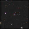 |
Fig. 1 Example training set image. The image size is 640 × 640, and the red box is a visualization of the label, which contains a dwarf galaxy sample. |
2.3 Data augmentation
Data augmentation is a commonly used technique in deep learning that generates more training samples by applying various transformations to the training data. Its main purpose is to improve the generalization ability of the model and reduce overfitting (Shorten & Khoshgoftaar 2019). After astronomical images are flipped and rotated, the physical properties and morphological structures of galaxies still retain their physical meaning. Additionally, galaxies can appear at any position within an image and are affected by instrumental and atmospheric disturbances. Based on the above analysis, we select four data augmentation methods: rotation, flipping, translation, and noise addition.
In most deep learning tasks, rotation and translation operations are applied directly to the training set, which results in a meaningless black background in the generated images and a loss of some image information (Kumar et al. 2024). In astronomical images, the background around celestial bodies and other negative sample celestial bodies have actual physical meanings, and their existence can help the model better distinguish dwarf galaxies from other celestial bodies. We wanted to use the real background to fill in the missing parts. Based on the above ideas, we designed a data augmentation method. A comparison of the augmentation methods is shown in Figure 2.
We use the dwarf galaxy sample as the centre of the image to obtain an image much larger than the training set. In order to ensure that the dwarf galaxy sample will not be truncated during the translation operation, we limit the maximum offset during translation according to the label. At the same time, considering that the image rotation cannot result in a black background under the maximum offset, we set the large image size to 2300 × 2300 based on experimental test results. We then fix a 640 × 640 bounding box at the centre of the image, and set a new label in the large image according to the label in Section 2.2. Next, we rotate and translate the image and update the position of the label and bounding box at the same time. Finally, we capture the image in the bounding box from the large image and then flip the captured image, and randomly perform Gaussian filtering or add noise to the image. The overall data augmentation process is illustrated in Figure 3.
Using the above augmentation strategy, we perform three rounds of augmentation on each image in the training set, expanding the training set from the original 1477 images to 5908 images.
3 Method
3.1 Structure of the YOLO-DG model
You Only Look Once (YOLO) (Redmon et al. 2016) is a deep learning algorithm designed for real-time object detection. Its core idea is to transform the object detection problem into a single regression task, enabling direct prediction from the image of the bounding box coordinates and category probabilities. Among the various versions of YOLO, YOLOv7 (Wang et al. 2023) has demonstrated excellent performance in a wide range of applications (Li et al. 2024; Liu et al. 2022; Yasir et al. 2024) Therefore, we chose YOLOv7 as the foundational framework for our model. To better search for and locate dwarf galaxies, we modified the YOLOv7 network and named the modified version YOLO-DG. The overall structure of YOLO-DG is shown in Figure 4.
The overall structure of YOLO-DG consists of three parts: Input, Backbone, and Head. The Input part is used to receive our input image data. In this study, our image specifications are 640 × 640 × 3. To address the problems of incomplete label information and a small number of samples, we perform data augmentation on the images before inputting them.
The Backbone component is responsible for extracting feature information from images. The Backbone component of YOLO-DG is similar to that of YOLOv7. To address the low resolution of faint dwarf galaxies, we introduce SPD-Conv (Sunkara & Luo 2023) to replace the strided convolution layer to reduce the loss of feature information and thus improve detection accuracy.
The Head component processes the feature information obtained from the Backbone, and outputs the final results. In YOLO-DG, the Head component adopts the path aggregation network (PANet) (Liu et al. 2018) structure. Although PANet effectively integrates the feature information of different scales, it lacks selective attention to various feature areas. To address this, we added coordinate attention (CA) (Hou et al. 2021) to the PANet structure. The CA embeds positional information into the channel, which enables the model to focus more on specific areas of the input data, thereby improving its understanding of the shape and spatial distribution of dwarf galaxies. The final output includes category information, confidence scores, and the position and size of the bounding boxes.
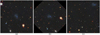 |
Fig. 2 Comparison of data augmentation strategies. (a) Training set image. (b) Image using conventional data augmentation strategy. (c) Image using YOLO-DG data augmentation strategy. |
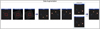 |
Fig. 3 Flow diagram of YOLO-DG data augmentation. |
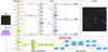 |
Fig. 4 Specific structure of the YOLO-DG network. The network structure can be divided into three parts: the Input module describes the image data, image dimensions, and preprocessing (Data augmentation); the Backbone and Head parts are the specific structure of YOLO-DG; the Result module is a visual display of the YOLO-DG result. The Structure of SPD-Conv module and the Structure of coordinate attention (CA) module below the figure respectively show the detailed structure of the modules we added. SPD-Conv consists of a space-to-depth (SPD) layer and a non-strided convolution layer, and CA consists of two parts: coordinate information embedding and coordinate attention generation. |
3.2 Loss function
The loss function used in YOLO-DG comprises three components: localization loss, Lloc, object confidence loss, Lobj, and classification loss, Lcls . The overall composition of the loss function is shown in Equation (1). The localization loss uses the CIoU (complete intersection over union) loss, as shown in Equation (2). The object confidence loss and classification loss use the BCE (binary cross-entropy) loss, as shown in Equation (6). The equations are as follows:
 (1)
(1)
 (2)
(2)
 (3)
(3)
 (4)
(4)
 (5)
(5)
![Mathematical equation: ${L_{BCE}} = - \left[ {{y_i}*\log \left( {\sigma \left( {{x_i}} \right)} \right) + \left( {1 - {y_i}} \right)*\log \left( {1 - \sigma \left( {{x_i}} \right)} \right)} \right],$](/articles/aa/full_html/2025/04/aa53042-24/aa53042-24-eq6.png) (6)
(6)
 (7)
(7)
In Equation (1), λ1, λ2, and λ3 represent the weights of different parts of the loss function, which are 0.05, 0.7, and 0.3, respectively, in this paper. In Equations (2)–(5), b denotes the predicted bounding box, bgt denotes the labelled bounding box, and ρ represents the Euclidean distance between the centre points of the two bounding boxes. The diagonal length of the smallest enclosing box that covers both bounding boxes is designated by c; α is a positive trade-off parameter, and v measures the consistency of the aspect ratio. The width and height of the predicted bounding box are represented by w and h, respectively, while the width and height of the labeled bounding box are denoted by wgt and hgt.
In Equation (6), xi represents the predicted value of the model output, and yi represents the true value. For classification loss, yi represents the true class of the training sample, and xi represents the predicted class of the object. For the object confidence loss, yi is the true confidence value, and xi is the predicted confidence value.
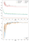 |
Fig. 5 Loss and evaluation metrics changes during YOLO-DG training. Top Panel: loss curve of YOLO-DG on the training set and validation set. As the number of the epoch increases, the loss gradually decreases and tends to be stable. Since we only detect dwarf galaxies, there is no classification loss. Bottom Panel: precision and recall rate change curve of YOLO-DG during training. |
3.3 Model evaluation
We use Precision (P) and Recall (R) to evaluate YOLO-DG, which are calculated as follows:
1. Precision (P):
 (8)
(8)
2. Recall (R):
 (9)
(9)
True positive (TP) indicates the number of positive samples correctly predicted as positive. False positive (FP) indicates the number of negative samples incorrectly predicted as positive. False negative (FN) indicates the number of positive samples incorrectly predicted as negative.
We use stochastic gradient descent during training, with the initial learning rate set to 0.01, and we do not use pre-trained weights. After 200 epochs of training, the loss converges, which results in a basic model capable of identifying dwarf galaxies. Figure 5 shows the changes in various indicators of YOLO-DG during the training process.
We used YOLO-DG to perform detection on the validation set and test set. In the validation set, 186 candidates were detected, of which 156 were known samples and 30 were new candidates, with a precision of 83.9% and a recall of 84.8%. In the test set, 186 candidates were also detected, of which 164 were known samples and 22 were new candidates, with a precision of 88.2% and a recall of 89.1%.
We converted the pixel coordinates of the detected new candidates into RA and Dec. Among the 30 new candidates detected in the validation set, 11 were identified as known dwarf galaxies. Similarly, among the 22 new candidates detected in the test set, 12 were identified as known dwarf galaxies. During the label making process, we only considered cases where there was a single dwarf galaxy in an image. Consequently, when multiple known dwarf galaxies were present in an image, YOLO- DG lacked the corresponding labels, which caused these known dwarf galaxies to be overlooked during evaluation.
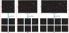 |
Fig. 6 Brick segmentation diagram. (a), (b), and (c) represent the cutting strategies for three bricks of different sizes. The three images at the top are images of the brick, and the corresponding images at the bottom are images after segmentation. The brick images here are downloaded from DESI in equal proportions for us to illustrate the cutting strategy, and are not complete bricks. We mark the size of the brick boundary and use red dotted lines to illustrate the cutting position. It can be seen that our cutting on the Dec boundary is unchanged, while the cutting on the RA boundary is set according to the size of the boundary. |
4 Search for dwarf galaxy candidates
4.1 DESI Data release 9 (DR9)
Data release 9 (DR9) includes BASS images taken from November 12, 2015 to March 7, 2019, MzLS images taken from November 19, 2015 to February 12, 2018, and DECaLS images taken from August 9, 2014 to March 7, 2019. For all of the DESI Legacy Imaging Surveys, images are presented in ‘bricks’ of an approximate size of 0.25° × 0.25°. Each brick is defined in terms of a box in RA, Dec coordinates2.
The pixel scale of the training set used for YOLO-DG is 0.262″/pix. In order to achieve the best search results, the pixel scale of the photometric image of the brick used in the search should be consistent. Therefore, the size of the photometric image of a complete brick is approximately 3436 × 3436. The maximum size of a single image that can be downloaded from DESI is 3000 × 3000, so we cut the bricks.
According to the catalogue provided by DESI, we can obtain the information of all bricks in the DR9 footprint, including the centre position of each brick and the upper and lower boundaries of RA and Dec. Based on the statistics of the contents of all bricks, we found that the Dec boundary size of all bricks is 0.25°, so all bricks are divided into two parts the Dec boundary, and the Dec boundary size of each cut image is 0.125°. The RA boundary sizes of all bricks is different, so we use 0.125° as the standard. If the RA boundary size is less than or equal to 0.25°, the RA boundary is evenly divided into two parts; if the length is greater than 0.25° and less than or equal to 0.375°, the RA boundary is evenly divided into three parts; if the length is greater than 0.375° and less than or equal to 0.5°, the RA boundary is evenly divided into four parts, and so on. Figure 6 shows how the bricks are segmented. Using the above cutting strategy, we divided a total of 332 041 bricks from DR9, ultimately obtaining 2 240 548 images.
4.2 Results analysis
We use YOLO-DG to detect dwarf galaxy candidates across the entire DR9 footprint. It takes 49.96 hours to process 2 240 548 images, with an average detection time of 0.0803 seconds per image. Since we cannot guarantee that each predicted bounding box detects a source accurately, we refer to the detection results as ‘targets’ for now. In total, we identify 916 748 targets.
We count the confidence scores of known dwarf galaxies detected in both the validation and test sets. Using the minimum confidence score as the threshold, we retain all targets with a confidence level above this threshold. Due to some overlap between bricks, some targets are detected multiple times. We use the centre position of each target’s bounding box as the standard, convert the pixel positions to their corresponding RA and Dec coordinates, and remove all targets with completely repeated positions. Finally, we are left with 865 215 targets in total. Figure 7 shows a schematic diagram of the search results obtained using YOLO-DG.
4.2.1 Properties of candidates
To obtain the properties of the candidates, we cross-match all targets with the DR9 Tractor Catalog, using a 5 arcsec distance as the matching criterion. If a target matches multiple sources within this distance, we select the closest source. Among the remaining 865 215 targets, 862 119 match the corresponding sources.
Based on the attributes of release, brickid, brickname, and objid, we find 115 220 duplicate sources in the cross-matched results. As previously noted, overlaps between bricks can cause YOLO-DG to produce duplicate detections if a target falls within these overlapping regions. The presence of bounding boxes can result in slight positional deviations, which leads to multiple targets matching the same source. We consider such targets as duplicate detections and remove them from our target samples. Consequently, the remaining 746 899 targets, which all match their corresponding sources, are considered valid candidates.
We cross-match the remaining 3096 targets that do not match the corresponding sources in the 865 215 targets with the DR10 Tractor Catalog using the same method. Among these 3096 targets, 706 targets matched the corresponding sources in DR10, including 45 duplicate sources.
We visually inspect the detection results of the remaining 2390 targets that still cannot be matched to a corresponding source in the DR10 Tractor Catalog and classify them into four types: (a) 42 erroneous targets resulting from incomplete or damaged photometric image data; (b) 1264 erroneous targets located towards one end of the astronomical object; (c) 675 targets too faint to be clearly distinguished by the naked eye; and (d) 100 targets that were clearly observed to be actual astronomical objects through visual inspection but were not identified by DESI. The results of the above four types of targets are the statistical results after we remove duplicate detections. Among the above 2390 targets, 309 are duplicate detections. Figure 8 shows example images from each type.
We regard (a) and (b) as invalid targets, so we will not discuss them further. For the target in type (c), we believe that there may be sources too faint to be identified by DR9, so we use SExtractor to determine whether the (c) type targets are background or real sources. After cross-matching the detection results of SExtractor with the (c) type targets within 5 arcsec, we identified 650 targets.
For targets in type (d), we also need to determine whether there is a real astronomical object at the target location. We believe that the reason why type (d) targets are not in the DESI Catalog may be that the cross-matching distance is small. Therefore, we first expand the cross-matching distance with the DESI Catalog. Considering that the cross-matching result may be wrong when the cross-matching distance is too large, we also visually inspect these sources in the DESI sky viewer. We find that these sources are completely inconsistent with our type (d) targets, so the cross-matching results are unreliable.
We cross-match the type (d) targets with the SDSS DR16 Catalog at 5 arcsec, and the results show that 26 type (d) targets match the corresponding sources. The cross-matching results confirm that there are real sources in the (d) type targets. Based on the type attribute in the SDSS, we find that these 26 targets are all galaxy class. Although there are still 74 targets in the (d) type that have not been matched to the source, based on the above cross-matching results with the SDSS and our visual inspection, we believe there is a high probability that these 74 targets are real sources, which can be confirmed through subsequent verification.
In DR9, there are six morphological types, five of which are used in the Tractor fitting procedure: point source (PSF), round exponential galaxies with a variable radius (REX), elliptical galaxies (DEV), spiral galaxies (EXP), and Sersic profiles (SER). The sixth morphological type, DUP, is set for Gaia sources. We count the morphological type of all candidates, with the results detailed in Table 2. Based on morphological type, we perform star-galaxy separation on all candidates, removing those in the PSF and DUP type. This leaves us with 742 251 dwarf galaxy candidates.
We calculate the magnitudes of all dwarf galaxy candidates based on the flux attribute of the Tractor Catalog. For the sake of comparison, we also calculated the magnitude of the training samples. The statistical results are shown in Figure 9. As can be seen from the figure, the magnitude distribution of the dwarf galaxy candidates detected by YOLO-DG is similar to that of the training samples, with peaks concentrated in the 19.020.0 mag range. This indicates that YOLO-DG has effectively learned the characteristics of the training set samples. In addition, our method has also discovered many fainter targets, which proves the superiority of our method.
Zhou et al. (2023) utilize the random forest algorithm to provide an updated set of photometric redshifts for all objects in DR9, as well as the spectral redshifts used for training. We compare our candidates with their complete catalogue and, based on the comparison, we divide the candidates into three parts: (i) 24 526 candidates with spectral redshifts; (ii) 707 906 candidates with photometric redshifts; and (iii) 9819 candidates without reasonable photometric redshifts.
Since Zhou et al. (2023) require at least one exposure in the g, r, and ɀ bands (NOBS_G,R,Z>1) when computing the photometric redshift, the category (iii) candidates do not meet the NOBS cut and thus their photometric redshifts are not provided. For category (iii) candidates, we use the photometric redshifts from Li et al. (2023) as a supplement, from which we obtain the photometric redshifts of 9818 candidates. For candidates with available spectral redshifts, we only count their spectral redshifts, for candidates without spectral redshifts, we only count their photometric redshifts, and for candidates with negative photometric redshift, we do not count their photometric redshifts. The statistical results are shown in Figure 10. In general, both spectral redshift and photometric redshift show heavy-tailed distribution. The redshifts of most dwarf galaxy candidates are small and concentrated around 0.1, which indicates that most of the dwarf galaxy candidates we detected are relatively close. As the redshift increases, the number of candidates gradually decreases, which means that more distant galaxies are more difficult to discover or detect due to weaker signals.
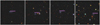 |
Fig. 7 Examples of YOLO-DG detection on DESI DR9. The bounding box marks the location of the target in the image, and the text content indicates the classification and confidence level of the object. |
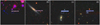 |
Fig. 8 Examples of a target that had no matching source. (a) is an erroneous detection due to incomplete or damaged photometric image data, (b) is an erroneous detection with a detection result that is towards one end of the astronomical object, (c) is a detection where the target is too faint to determine whether it is a real source, and (d) is a source that is confirmed to be a real astronomical object by visual inspection but is not in the DESI Tractor Catalog. |
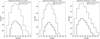 |
Fig. 9 Magnitude distribution of dwarf galaxy candidates and training samples in the g, r, and ɀ bands. Since there are a large number of dwarf galaxy candidates, we take the logarithm of the number for easy comparison. |
Morphological type statistics of all candidates.
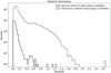 |
Fig. 10 Redshift distribution of dwarf galaxy candidates. If a dwarf galaxy candidate has a spectral redshift, we do not count its photometric redshift. Due to the large number of candidates, we present the number in logarithmic form. |
4.2.2 Local volume dwarf galaxy candidates
Creating a complete catalogue of dwarf galaxy candidates in the nearest area of the universe can provide an important observational basis for testing small-scale cosmological models. The local volume is defined as a spherical region with a radius of 10 megaparsecs from Earth (Koribalski et al. 2018). We use a redshift of less than 0.0023 as the criterion for identifying local volume dwarf galaxy candidates.
For candidates with spectral redshifts, we directly identify local volume dwarf galaxy candidates based on their redshift. For candidates with photometric redshifts, we take the error into account. For the photometric redshift from Zhou et al. (2023), the normalized median absolute deviation σNMAD is used as the error, and the σNMAD of all training datasets is provided. We sum the σNMAD in each training set and take the average as the error we use. If the value of the photometric redshift of a candidate minus the average error is less than 0.0023, we consider the candidate to be a local volume dwarf galaxy candidate. For the photometric redshift of Li et al. (2023), the paper directly provides σNMAD. Similarly, if the value of the photometric redshift of a candidate minus the average error is less than 0.0023, we consider the candidate to be a local volume dwarf galaxy candidate.
Based on the above criteria, we identify 95 230 local volume dwarf galaxy candidates, 33 of which are confirmed through spectral redshifts. Examples of these candidates are presented in Figure 11. Additionally, we plotted the CMD for the local volume dwarf galaxy candidates, with the results shown in Figure 12. From the overall perspective of the figure, the data points show a distribution trend from the upper right to the lower left. From the distribution of the half-light radius of the galaxies, most galaxies have a small half-light radius and are likely to be compact galaxies whose luminosity is mainly concentrated in the central region. A small number of galaxies with larger halflight radii are distributed in the lower middle part of the figure, which indicates that these galaxies have larger physical sizes and may be nearby disc galaxies or elliptical galaxies with significant extended structures.
We provide two complete catalogues: one for local volume dwarf galaxy candidates identified through spectral redshifts and another for those identified through photometric redshifts. An example catalogue is shown in Table 3.
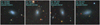 |
Fig. 11 Examples of local volume dwarf galaxy candidate image. The coordinates and redshift information of the candidate are given in the upper left corner. |
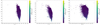 |
Fig. 12 Colour magnitude diagram of the local volume dwarf galaxy candidates. The depth of the point colour indicates the length of the candidate’s half-light radius: the darker the colour, the smaller the half-light radius. |
5 Summary
In this paper, we propose an end-to-end automatic identification scheme for dwarf galaxies and provide a batch of local volume dwarf galaxy candidates. We develop a dwarf galaxy detection model, YOLO-DG, to search for and directly locate dwarf galaxy candidates in DESI photometric images. We construct a deep learning dataset for dwarf galaxies and design a data augmentation method specifically for them. YOLO-DG achieves a precision of 88.2% and a recall of 89.1% on the test set. We used YOLO-DG to detect across the entire DESI DR9 footprint and identified 746 899 candidates. From the analysis of the magnitude results, YOLO-DG can detect targets that exceed the DESI fiducial depth.
Based on the morphological classification of the candidates, we identify 742 251 dwarf galaxy candidates, which represents 99.38% of all candidates. Out of these, we confirm 95 230 as local volume dwarf galaxy candidates, with 33 confirmed through spectral redshifts. Structurally, the smallest local volume dwarf galaxy candidate has a half-light radius of 0.31 arcsec.
Although our research has achieved satisfactory results, like most supervised deep learning methods, YOLO-DG is limited by our training set and focuses on faint and small size dwarf galaxies. In the future, we can expand the detection capabilities by enriching the training set. By improving this method, it can be utilized in the next generation of sky surveys to provide new dwarf galaxy samples, thereby advancing research on the missing satellite problem to a significant extent.
Example catalog of local volume dwarf galaxy candidates
Data availability
All tables are only available in electronic form at the CDS via anonymous ftp to cdsarc.cds.unistra.fr (130.79.128.5) or via https://cdsarc.cds.unistra.fr/viz-bin/cat/J/A+A/696/A130.
Acknowledgements
The work is supported by the National Natural Science Foundation of China (Grant Nos. 12473105, 12473106, 62272336), Projects of Science and Technology Cooperation and Exchange of Shanxi Province (Grant Nos. 202204041101037, 202204041101033), The central government guides local funds for science and technology development (YDZJSX2024D049), the science research grant from the China Manned Space Project with No. CMS-CSST- 2021-B03, and Guanghe Fund (No. ghfund2O24O7O2749O). The DESI Legacy Imaging Surveys consist of three individual and complementary projects: the Dark Energy Camera Legacy Survey (DECaLS), the Beijing-Arizona Sky Survey (BASS), and the Mayall ɀ-band Legacy Survey (MzLS). DECaLS, BASS and MzLS together include data obtained, respectively, at the Blanco telescope, Cerro Tololo Inter-American Observatory, NSF’s NOIRLab; the Bok telescope, Steward Observatory, University of Arizona; and the Mayall telescope, Kitt Peak National Observatory, NOIRLab. NOIRLab is operated by the Association of Universities for Research in Astronomy (AURA) under a cooperative agreement with the National Science Foundation. Pipeline processing and analyses of the data were supported by NOIRLab and the Lawrence Berkeley National Laboratory (LBNL). Legacy Surveys also uses data products from the Near-Earth Object Wide-field Infrared Survey Explorer (NEOWISE), a project of the Jet Propulsion Laboratory/California Institute of Technology, funded by the National Aeronautics and Space Administration. Legacy Surveys was supported by: the Director, Office of Science, Office of High Energy Physics of the U.S. Department of Energy; the National Energy Research Scientific Computing Center, a DOE Office of Science User Facility; the U.S. National Science Foundation, Division of Astronomical Sciences; the National Astronomical Observatories of China, the Chinese Academy of Sciences and the Chinese National Natural Science Foundation. LBNL is managed by the Regents of the University of California under contract to the U.S. Department of Energy. The complete acknowledgments can be found at https://www.legacysurvey.org/acknowledgment/. The Photometric Redshifts for the Legacy Surveys (PRLS) catalog used in this paper was produced thanks to funding from the U.S. Department of Energy Office of Science, Office of High Energy Physics via grant DE-SC0007914.
References
- Annibali, F., & Tosi, M. 2022, Nat. Astron., 6, 48 [NASA ADS] [CrossRef] [Google Scholar]
- Belokurov, V., Zucker, D. B., Evans, N. W., et al. 2006, ApJ, 647, L111 [NASA ADS] [CrossRef] [Google Scholar]
- Belokurov, V., Zucker, D. B., Evans, N. W., et al. 2007, ApJ, 654, 897 [Google Scholar]
- Belokurov, V., Walker, M. G., Evans, N. W., et al. 2008, ApJ, 686, L83 [NASA ADS] [CrossRef] [Google Scholar]
- Bertin, E., & Arnouts, S. 1996, A&AS, 117, 393 [NASA ADS] [CrossRef] [EDP Sciences] [Google Scholar]
- Bullock, J. S. 2010, ArXiv e-prints [arXiv:1009.4505] [Google Scholar]
- Bullock, J. S., & Boylan-Kolchin, M. 2017, ARA&A, 55, 343 [Google Scholar]
- Byun, W., Sheen, Y.-K., Park, H. S., et al. 2020, ApJ, 891, 18 [NASA ADS] [CrossRef] [Google Scholar]
- Cai, J., Yan, Z., Yang, H., et al. 2024, A&A, 687, A15 [NASA ADS] [CrossRef] [EDP Sciences] [Google Scholar]
- Cao, Z., Yi, Z., Pan, J., et al. 2023, AJ, 165, 184 [Google Scholar]
- Cerny, W., Pace, A. B., Drlica-Wagner, A., et al. 2021, ApJ, 920, L44 [NASA ADS] [CrossRef] [Google Scholar]
- Choque-Challapa, N., Aguerri, J. A. L., Mancera Piña, P. E., et al. 2021, MNRAS, 507, 6045 [NASA ADS] [CrossRef] [Google Scholar]
- Collins, M. L. M., Charles, E. J. E., Martínez-Delgado, D., et al. 2022, MNRAS, 515, L72 [NASA ADS] [CrossRef] [Google Scholar]
- Crosby, E., Jerjen, H., Müller, O., et al. 2024, MNRAS, 527, 9118 [Google Scholar]
- Davies, J. I., Davies, L. J. M., & Keenan, O. C. 2016, MNRAS, 456, 1607 [Google Scholar]
- Dey, A., Schlegel, D. J., Lang, D., et al. 2019, AJ, 157, 168 [Google Scholar]
- Homma, D., Chiba, M., Komiyama, Y., et al. 2024, PASJ, 76, 733 [NASA ADS] [CrossRef] [Google Scholar]
- Hou, Q., Zhou, D., & Feng, J. 2021, in 2021 IEEE/CVF Conference on Computer Vision and Pattern Recognition (CVPR), 13708 [CrossRef] [Google Scholar]
- Karachentsev, I. D., Makarov, D. I., & Kaisina, E. I. 2013, AJ, 145, 101 [Google Scholar]
- Klypin, A., Kravtsov, A. V., Valenzuela, O., & Prada, F. 1999, ApJ, 522, 82 [Google Scholar]
- Koribalski, B. S., Wang, J., Kamphuis, P., et al. 2018, MNRAS, 478, 1611 [NASA ADS] [CrossRef] [Google Scholar]
- Kumar, T., Brennan, R., Mileo, A., & Bendechache, M. 2024, IEEE Access, 12, 187536 [Google Scholar]
- La Marca, A., Peletier, R., Iodice, E., et al. 2022, A&A, 659, A92 [NASA ADS] [CrossRef] [EDP Sciences] [Google Scholar]
- LeCun, Y., Bengio, Y., & Hinton, G. 2015, Nature, 521, 436 [Google Scholar]
- Li, C., Zhang, Y., Cui, C., et al. 2023, MNRAS, 518, 513 [Google Scholar]
- Li, Q., Ma, W., Li, H., et al. 2024, Comp. Electron. Agri., 219, 108752 [Google Scholar]
- Liu, S., Qi, L., Qin, H., Shi, J., & Jia, J. 2018, in 2018 IEEE/CVF Conference on Computer Vision and Pattern Recognition, 8759 [CrossRef] [Google Scholar]
- Liu, S., Wang, Y., Yu, Q., Liu, H., & Peng, Z. 2022, IEEE Access, 10, 129116 [CrossRef] [Google Scholar]
- Madden, S. C. & Cormier, D. 2019, IAU Symp., 344, 240 [Google Scholar]
- Martin, N. F., McConnachie, A. W., Irwin, M., et al. 2009, ApJ, 705, 758 [NASA ADS] [CrossRef] [Google Scholar]
- Martínez-Delgado, D., Makarov, D., Javanmardi, B., et al. 2021, A&A, 652, A48 [NASA ADS] [CrossRef] [EDP Sciences] [Google Scholar]
- Martínez-Delgado, D., Karim, N., Charles, E. J. E., et al. 2022, MNRAS, 509, 16 [Google Scholar]
- Mau, S., Cerny, W., Pace, A. B., et al. 2020, ApJ, 890, 136 [NASA ADS] [CrossRef] [Google Scholar]
- McConnachie, A. W., Huxor, A., Martin, N. F., et al. 2008, ApJ, 688, 1009 [NASA ADS] [CrossRef] [Google Scholar]
- Müller, O., Jerjen, H., & Binggeli, B. 2015, A&A, 583, A79 [NASA ADS] [CrossRef] [EDP Sciences] [Google Scholar]
- Müller, O., Rejkuba, M., Pawlowski, M. S., et al. 2019, A&A, 629, A18 [Google Scholar]
- Mutlu-Pakdil, B., Sand, D. J., Crnojević, D., et al. 2022, ApJ, 926, 77 [NASA ADS] [CrossRef] [Google Scholar]
- Park, H. S., Moon, D.-S., Zaritsky, D., et al. 2017, ApJ, 848, 19 [NASA ADS] [CrossRef] [Google Scholar]
- Perivolaropoulos, L., & Skara, F. 2022, New A Rev., 95, 101659 [NASA ADS] [CrossRef] [Google Scholar]
- Poulain, M., Marleau, F. R., Habas, R., et al. 2021, MNRAS, 506, 5494 [NASA ADS] [CrossRef] [Google Scholar]
- Redmon, J., Divvala, S., Girshick, R., & Farhadi, A. 2016, in 2016 IEEE Conference on Computer Vision and Pattern Recognition (CVPR) (Los Alamitos, CA, USA: IEEE Computer Society), 779 [CrossRef] [Google Scholar]
- Reefe, M., Satyapal, S., Sexton, R. O., et al. 2023, ApJ, 946, L38 [NASA ADS] [CrossRef] [Google Scholar]
- Saremi, E., Javadi, A., van Loon, J. T., et al. 2020, ApJ, 894, 135 [Google Scholar]
- Shi, J.-H., Qiu, B., Luo, A. L., et al. 2022, MNRAS, 516, 264 [Google Scholar]
- Shorten, C., & Khoshgoftaar, T. 2019, J. Big Data, 6, 60 [CrossRef] [Google Scholar]
- Sunkara, R., & Luo, T. 2023, in Machine Learning and Knowledge Discovery in Databases, eds. M.-R. Amini, S. Canu, A. Fischer, (Cham: Springer Nature Switzerland), 443 [Google Scholar]
- Teeninga, P., Moschini, U., Trager, S. C., & Wilkinson, M. H. F. 2015, in Mathematical Morphology and Its Applications to Signal and Image Processing, eds. J. A. Benediktsson, J. Chanussot, L. Najman, & H. Talbot (Cham: Springer International Publishing), 157 [Google Scholar]
- Tolstoy, E. 2003, Ap&SS, 284, 579 [Google Scholar]
- Torrealba, G., Koposov, S. E., Belokurov, V., & Irwin, M. 2016, MNRAS, 459, 2370 [NASA ADS] [CrossRef] [Google Scholar]
- Torrealba, G., Belokurov, V., Koposov, S. E., et al. 2018, MNRAS, 475, 5085 [NASA ADS] [CrossRef] [Google Scholar]
- Torrealba, G., Belokurov, V., Koposov, S. E., et al. 2019, MNRAS, 488, 2743 [NASA ADS] [CrossRef] [Google Scholar]
- Venhola, A., Peletier, R., Laurikainen, E., et al. 2018, A&A, 620, A165 [NASA ADS] [CrossRef] [EDP Sciences] [Google Scholar]
- Venhola, A., Peletier, R. F., Salo, H., et al. 2022, A&A, 662, A43 [NASA ADS] [CrossRef] [EDP Sciences] [Google Scholar]
- Wang, C.-Y., Bochkovskiy, A., & Liao, H.-Y. M. 2023, in 2023 IEEE/CVF Conference on Computer Vision and Pattern Recognition (CVPR), 7464 [CrossRef] [Google Scholar]
- Willman, B., Blanton, M. R., West, A. A., et al. 2005a, AJ, 129, 2692 [NASA ADS] [CrossRef] [Google Scholar]
- Willman, B., Dalcanton, J. J., Martinez-Delgado, D., et al. 2005b, ApJ, 626, L85 [Google Scholar]
- Yang, H., Shi, C., Cai, J., et al. 2022, MNRAS, 517, 5496 [NASA ADS] [CrossRef] [Google Scholar]
- Yang, H., Zhou, L., Cai, J., et al. 2023a, MNRAS, 518, 5904 [Google Scholar]
- Yang, H.-F., Yin, X.-N., Cai, J.-H., et al. 2023b, Res. Astron. Astrophys., 23, 055006 [CrossRef] [Google Scholar]
- Yang, H.-F., Wang, R., Cai, J.-H., et al. 2024, ApJS, 272, 43 [NASA ADS] [CrossRef] [Google Scholar]
- Yasir, M., Shanwei, L., Mingming, X., et al. 2024, Appl. Soft Comp., 160, 111704 [Google Scholar]
- Yi, Z., Li, J., Du, W., et al. 2022, MNRAS, 513, 3972 [NASA ADS] [CrossRef] [Google Scholar]
- Zhou, R., Ferraro, S., White, M., et al. 2023, J. Cosmology Astropart. Phys., 2023, 097 [Google Scholar]
All Tables
All Figures
|
Fig. 1 Example training set image. The image size is 640 × 640, and the red box is a visualization of the label, which contains a dwarf galaxy sample. |
| In the text | |
|
Fig. 2 Comparison of data augmentation strategies. (a) Training set image. (b) Image using conventional data augmentation strategy. (c) Image using YOLO-DG data augmentation strategy. |
| In the text | |
|
Fig. 3 Flow diagram of YOLO-DG data augmentation. |
| In the text | |
|
Fig. 4 Specific structure of the YOLO-DG network. The network structure can be divided into three parts: the Input module describes the image data, image dimensions, and preprocessing (Data augmentation); the Backbone and Head parts are the specific structure of YOLO-DG; the Result module is a visual display of the YOLO-DG result. The Structure of SPD-Conv module and the Structure of coordinate attention (CA) module below the figure respectively show the detailed structure of the modules we added. SPD-Conv consists of a space-to-depth (SPD) layer and a non-strided convolution layer, and CA consists of two parts: coordinate information embedding and coordinate attention generation. |
| In the text | |
|
Fig. 5 Loss and evaluation metrics changes during YOLO-DG training. Top Panel: loss curve of YOLO-DG on the training set and validation set. As the number of the epoch increases, the loss gradually decreases and tends to be stable. Since we only detect dwarf galaxies, there is no classification loss. Bottom Panel: precision and recall rate change curve of YOLO-DG during training. |
| In the text | |
|
Fig. 6 Brick segmentation diagram. (a), (b), and (c) represent the cutting strategies for three bricks of different sizes. The three images at the top are images of the brick, and the corresponding images at the bottom are images after segmentation. The brick images here are downloaded from DESI in equal proportions for us to illustrate the cutting strategy, and are not complete bricks. We mark the size of the brick boundary and use red dotted lines to illustrate the cutting position. It can be seen that our cutting on the Dec boundary is unchanged, while the cutting on the RA boundary is set according to the size of the boundary. |
| In the text | |
|
Fig. 7 Examples of YOLO-DG detection on DESI DR9. The bounding box marks the location of the target in the image, and the text content indicates the classification and confidence level of the object. |
| In the text | |
|
Fig. 8 Examples of a target that had no matching source. (a) is an erroneous detection due to incomplete or damaged photometric image data, (b) is an erroneous detection with a detection result that is towards one end of the astronomical object, (c) is a detection where the target is too faint to determine whether it is a real source, and (d) is a source that is confirmed to be a real astronomical object by visual inspection but is not in the DESI Tractor Catalog. |
| In the text | |
|
Fig. 9 Magnitude distribution of dwarf galaxy candidates and training samples in the g, r, and ɀ bands. Since there are a large number of dwarf galaxy candidates, we take the logarithm of the number for easy comparison. |
| In the text | |
|
Fig. 10 Redshift distribution of dwarf galaxy candidates. If a dwarf galaxy candidate has a spectral redshift, we do not count its photometric redshift. Due to the large number of candidates, we present the number in logarithmic form. |
| In the text | |
|
Fig. 11 Examples of local volume dwarf galaxy candidate image. The coordinates and redshift information of the candidate are given in the upper left corner. |
| In the text | |
|
Fig. 12 Colour magnitude diagram of the local volume dwarf galaxy candidates. The depth of the point colour indicates the length of the candidate’s half-light radius: the darker the colour, the smaller the half-light radius. |
| In the text | |
Current usage metrics show cumulative count of Article Views (full-text article views including HTML views, PDF and ePub downloads, according to the available data) and Abstracts Views on Vision4Press platform.
Data correspond to usage on the plateform after 2015. The current usage metrics is available 48-96 hours after online publication and is updated daily on week days.
Initial download of the metrics may take a while.