| Issue |
A&A
Volume 695, March 2025
|
|
|---|---|---|
| Article Number | A246 | |
| Number of page(s) | 13 | |
| Section | Cosmology (including clusters of galaxies) | |
| DOI | https://doi.org/10.1051/0004-6361/202452119 | |
| Published online | 25 March 2025 | |
YOLO-CL cluster detection in the Rubin/LSST DC2 simulations
1
Université Paris Cité, CNRS(/IN2P3), Astroparticule et Cosmologie, F-75013 Paris, France
2
CNRS-UCB International Research Laboratory, Centre Pierre Binétruy, IRL2007, CPB-IN2P3, Berkeley, USA
3
Jet Propulsion Laboratory and Cahill Center for Astronomy & Astrophysics, California Institute of Technology, 4800 Oak Grove Drive, Pasadena, California 91011, USA
4
IJCLab, Université Paris-Saclay, CNRS/IN2P3, IJCLab, 91405 Orsay, France
5
LAPP, Université Savoie Mont Blanc, CNRS/IN2P3, Annecy, France
⋆ Corresponding authors; This email address is being protected from spambots. You need JavaScript enabled to view it.
; This email address is being protected from spambots. You need JavaScript enabled to view it.
Received:
5
September
2024
Accepted:
17
January
2025
Abstract
The next generation large ground-based telescopes like the Vera Rubin Telescope Legacy Survey of Space and Time (LSST) and space missions like Euclid and the Nancy Roman Space Telescope will deliver wide area imaging surveys at unprecedented depth. In particular, LSST will provide galaxy cluster catalogs up to z ∼ 1 that can be used to constrain cosmological models once their selection function is well-understood. Machine learning based cluster detection algorithms can be applied directly on images to circumvent systematics due to models and photometric and photometric redshift catalogs. In this work, we have applied the deep convolutional network YOLO for CLuster detection (YOLO-CL) to LSST simulations from the Dark Energy Science Collaboration Data Challenge 2 (DC2), and characterized the LSST YOLO-CL cluster selection function. We have trained and validated the network on images from a hybrid sample of (1) clusters observed in the Sloan Digital Sky Survey and detected with the red-sequence Matched-filter Probabilistic Percolation, and (2) dark matter halos with masses M200c > 1014 M⊙ from the DC2 simulation, resampled to the SDSS resolution. We quantify the completeness and purity of the YOLO-CL cluster catalog with respect to DC2 halos with M200c > 1014 M⊙. The YOLO-CL cluster catalog is 100% and 94% complete for halo mass M200c > 1014.6 M⊙ at 0.2 < z < 0.8, and M200c > 1014 M⊙ and redshift z ≲ 1, respectively, with only 6% false positive detections. We find that all the false positive detections are dark matter halos with 1013.4 M⊙ ≲ M200c ≲ 1014 M⊙, which corresponds to galaxy groups. We also found that the YOLO-CL selection function is almost flat with respect to the halo mass at 0.2 ≲ z ≲ 0.9. The overall performance of YOLO-CL is comparable or better than other cluster detection methods used for current and future optical and infrared surveys. YOLO-CL shows better completeness for low mass clusters when compared to current detections based on Matched Filter cluster finding algorithms applied to Stage 3 surveys using the Sunyaev Zel’dovich effect, such as SPT-3G, and detects clusters at higher redshifts than X-ray-based catalogs. Future complementary cluster catalogs detected with the Sunyaev Zel’dovich effect will reach similar mass depth and will be directly comparable with optical cluster detections in LSST, providing cluster catalogs with unprecedented coverage in area, redshift and cluster properties. The strong advantage of YOLO-CL over traditional galaxy cluster detection techniques is that it works directly on images and does not require photometric and photometric redshift catalogs, nor does it need to mask stellar sources and artifacts.
Key words: cosmology: observations / large-scale structure of Universe
© The Authors 2025
 Open Access article, published by EDP Sciences, under the terms of the Creative Commons Attribution License (https://creativecommons.org/licenses/by/4.0), which permits unrestricted use, distribution, and reproduction in any medium, provided the original work is properly cited.
This article is published in open access under the Subscribe to Open model. This email address is being protected from spambots. You need JavaScript enabled to view it. to support open access publication.
1. Introduction
Galaxy clusters are the largest gravitationally bound structures in the Universe, and their distribution is a probe for cosmological models. Upcoming deep large-scale surveys such as those performed with the Vera C. Rubin Observatory (Kahn 2018), the Euclid space telescope (Laureijs et al. 2011) and the Nancy Grace Roman Space Telescope (Eifler et al. 2021) will give us unprecedented deep optical and infrared imaging of hundreds of thousands of clusters up to z ∼ 2.
In particular, the Vera Rubin Telescope Legacy Survey of Space and Time (LSST; LSST Science Collaboration 2009; Ivezić et al. 2019) will deliver deep optical imaging data over ∼20 000 sq. deg. of the sky. LSST will observe in six bandpasses (u, g, r, i, z, y) and reach a depth of r ∼ 27.5 mag over about half of the sky (Olivier et al. 2012, 2006). These observations will permit us to obtain constraints on cosmological models using galaxy clusters, once we can provide a precise selection function.
Cluster detection in optical and near-infrared multiwavelength imaging surveys is mainly based on the search for spatial overdensities of galaxies of a given class, which can be quiescent, line-emitter, massive, and so on (e.g., Gladders & Yee 2005; Koester et al. 2007; Knobel et al. 2009; Wen et al. 2009, 2012; Sobral et al. 2010; Hao et al. 2010; Szabo et al. 2011; Muzzin et al. 2012; Bayliss et al. 2011; Wylezalek et al. 2013, 2014; Rykoff et al. 2014; Mei et al. 2015; Licitra et al. 2016a,b; Maturi et al. 2019; Werner et al. 2023). Most of these methods require a high-quality photometric calibration, an accurate calibration of galaxy colors as a function of redshift, and unbiased photometric and photometric redshift catalogs. Photometric catalogs might be affected by aperture or model choices in measuring magnitudes and background subtraction. These systematics propagate to the estimation of photometric redshifts, which also rely on being calibrated on available spectroscopic redshift samples and galaxy spectral energy distribution templates that do not cover the entire galaxy population (e.g., Moskowitz et al. 2024). These uncertainties on both photometric and photometric redshift catalogs make it essential to complement traditional cluster detection algorithms with new techniques that do not rely on catalogs but instead work directly on images, such as deep machine learning (ML) neural networks.
Over the last few years, deep ML techniques have been widely used in astrophysics for different purposes (Huertas-Company & Lanusse 2023), including object classification (Domínguez Sánchez et al. 2018; Angora et al. 2023), estimating the redshift of individual galaxies (Pasquet et al. 2019; Henghes et al. 2021), and solving ill-posed problems, including reconstructions of matter distributions (Jeffrey et al. 2020; Cornu et al. 2024; Chen et al. 2023). The purity of the samples, defined as the percentage of true objects recovered by the network as opposite to false detections, was high enough to search for rare or elusive objects (Hezaveh et al. 2017; Cornu & Montillaud 2021). Among these methods, convolutional neural networks (CNN) are well adapted for object detection and characterization in astrophysics (e.g., Huertas-Company et al. 2015, 2018; Dimauro et al. 2018; Pasquet et al. 2019; Zanisi et al. 2021; Davidzon et al. 2022; Euclid Collaboration: Bretonnière et al. 2022; Euclid Collaboration: Bisigello et al. 2023a; Euclid Collaboration: Humphrey et al. 2023b), and in particular galaxy cluster detection (e.g., Chan & Stott 2019; Bonjean 2020; Hurier et al. 2021; Lin et al. 2021; Grishin et al. 2023).
Recently, our team developed a cluster detection method modifying the well-known detection-oriented deep ML neural network “You only look once” (YOLO, Redmon et al. 2015; Redmon & Farhadi 2016). Our network, YOLO-CL (YOLO for CLuster detection; Grishin et al. 2023), detects galaxy clusters on multiwavelength images, and shows a higher performance with respect to traditional cluster detection algorithms in obtaining cluster catalogs with high completeness and purity. When applied to the Sloan Digital Sky Survey (SDSS; York et al. 2000), YOLO-CL provides cluster catalogs that are ∼98% complete for X-ray detected clusters with IX, 500 ≳ 20 × 10−15 erg/s/cm2/arcmin2 at 0.2 ≲ z ≲ 0.6, and ∼100% complete for clusters with IX, 500 ≳ 30 × 10−15 erg/s/cm2/arcmin2 at 0.3 ≲ z ≲ 0.6. The contamination from false detections is ∼2%. It is also interesting that Grishin et al. (2023) found that the YOLO-CL selection function is flat as a function of redshift, with respect to the X-ray mean surface brightness. The advantage of YOLO-CL, and other ML networks that work directly on images, is that they are independent of models and systematics that might arise when building photometric and photometric redshift catalogs in traditional methods. They also do not need stellar sources and artifacts to be masked. If the training sample is representative of the entire observed sample, the ML methods should be less impacted by modeling choices and systematics.
In this paper, we evaluate the YOLO-CL efficiency in detecting galaxy clusters in the LSST survey. Given that LSST observations have not yet started, we applied the network to simulations from the LSST Data Challenge 2 (DC2; LSST Dark Energy Science Collaboration (LSST DESC) 2021) that were developed within the LSST Dark Energy Science Collaboration (DESC1). We quantified the YOLO-CL cluster catalog selection function in terms of completeness and purity (see below) with respect to DC2 halos with M200c > 1014 M⊙. The YOLO-CL cluster catalog is 100% complete for a halo mass of M200c > 1014.6 M⊙ at 0.2 < z < 0.8, and 94% complete for M200c > 1014 M⊙ and redshift z ≲ 1, with only 6% false positive detections. This contamination is expected from the intrinsic accuracy of CNN, and our network is highly efficient with respect to traditional cluster detection algorithms based on photometric and photometric redshift catalogs. It is interesting that all the false positive detections are groups with 1013.4 M⊙ ≲ M200c ≲ 1014 M⊙, and that the catalog selection function is flat with respect to the halo mass at 0.2 ≲ z ≲ 0.9.
This article is organized as follows: in Sect. 2.2 we describe the observations and simulations used to train and validate our network. In Sect. 3 we present YOLO-CL and its training and validation. The results are presented in Sect. 4 and the discussion in Sect. 5. The summary is in Sect. 6. All magnitudes are given in the AB system (Oke & Gunn 1983; Sirianni et al. 2005). We adopt a ΛCDM cosmology, with ΩM = 0.3, ΩΛ = 0.7, h = 0.72, and σ8 = 0.8.
2. Observations and simulations
Since the DESC DC2 simulated area includes only ≈ 2000 synthetic galaxy clusters (see Sect. 2.2) and we need at least 10 000 objects for training our network, we trained YOLO-CL on a hybrid sample of cluster images that includes both the same set of SDSS observed images (Abazajian et al. 2009) that we used in Grishin et al. (2023), and synthetic cluster images from the DESC DC2 simulations. In fact, the simple use of the SDSS-only trained YOLO-CL weights from Grishin et al. (2023) applied to LSST simulations was not very efficient in recovering high completeness and purity catalogs.
This transfer learning strategy is widely used in astrophysics when the target sample (in our case the LSST DC2 simulations) is large enough to provide a statistical application of a network, but too small to be used for the network training and validation. In the case of convolutional networks, such as YOLO-CL, Domínguez Sánchez et al. (2018) demonstrate that transfer learning allows for rapid adaptation from one astrophysical survey application to another. Specifically, the weights obtained by training a convolutional network on images from a given survey can be efficiently transferred to another survey by fine-tuning them; that is, by retraining the network adding a smaller number of images from the new survey, roughly an order of magnitude fewer than the initial training sample. In their case, the initial survey was SDSS, and they applied transfer learning to the Dark Energy Survey (Abbott et al. 2018). We demonstrate in this section that this approach is also effective when retraining YOLO-CL using our initial training set from SDSS, which was utilized in Grishin et al. (2023), and incorporating approximately one order of magnitude fewer synthetic cluster images from the DESC DC2 simulations. As is described below (sec 2.2), we made sure to generate DC2 composite color images consistent with SDSS images in terms of resolution and depth.
2.1. The SDSS observations
The SDSS is an imaging survey that was performed with the 2.5-m. Apache Point telescope in five optical bandpasses (u, g, r, i, z) using the SDSS camera in a scanning regime. It covers ∼14 055 sq. deg. of the sky in two main areas in the northern hemisphere split by the Milky Way: one within 7 h < RA < 16 h and −1 deg < Dec < +62 deg and the other within 20 h < RA < 2 h and −11 deg < Dec < +35 deg. The 5-σ point-source depth in the g, r, and i bandpasses is 23.13, 22.70, and 22.20 mag, respectively. The seeing quality for SDSS images varies from 1.2 to 2.0 arcsec2.
As a reference SDSS cluster catalog, we used the red-sequence matched-filter probabilistic percolation (redMaPPer) Data Release 8 (DR8) catalog from Rykoff et al. (2014). The redMaPPer algorithm finds overdensities of red-sequence galaxies in large photometric surveys. The cluster catalog that we used3 covers ∼10 000 square degrees of the SDSS DR8 data release, and includes 26 111 clusters over the redshift range z ∈ [0.08, 0.55] and richness λ> 20. The redMaPPer catalog is 100% complete up to z = 0.35 for clusters from the MCXC (Meta-Catalog of X-Ray Detected Clusters of Galaxies) X-ray detection catalog (Piffaretti et al. 2011), with a temperature of TX ≳ 3.5keV and luminosity of LX ≳ 2 × 1044 erg s−1, decreasing to 90% completeness at LX ∼ 1043 erg s−1. Rykoff et al. (2014) also find that redMaPPer recovers the central galaxy that they identified via visual inspection 86.0% ± 3.2% of the time. For each cluster, redMaPPer provides its position, the richness λ4, and a list of cluster members. The richness correlats to the cluster mass. All redMaPPer rich clusters (λ > 100) were detected in the X-ray ROSAT All Sky Survey (Voges et al. 1999).
We excluded clusters with redshifts of z < 0.2 from the original redMaPPer cluster catalog, because they cover regions in the sky larger than the images that we consider when optimizing our network execution time and computational power (see Sect. 3.2). Our final redMaPPer catalog includes 24 406 clusters, whose distribution is shown in Fig. 1 from Grishin et al. (2023).
For the network training and validation, we used JPEG color images of the original SDSS DR16 images centered on each of the 24 406 redMaPPer clusters, using the ImgCutout web service5. These images were derived from the g, r, and i-band corrected frame files from the Science Archive Server, and the color images were built using the conversion algorithm6 based on Lupton et al. (2004). We chose these three bandpasses because they are sufficient to identify passive early-type galaxies in clusters at z ≲ 1.
2.2. The DESC DC2 simulation
In ten years, LSST will reach the 5-σ point-source depth of 27.4, 27.5, and 26.8 mag in the g, r and i bandpasses, respectively (Ivezić et al. 2019). This will allow to build a catalog of 20 billion individual galaxies, and over 100 000 galaxy clusters at z < 1.2. The average seeing quality at the Rubin telescope site is 0.67″ with a best value of 0.4″, which is very close to the best spatial resolution that can be achieved from the ground.
The primary goal of the LSST DESC DC2 simulation is to create realistic LSST synthetic observations that can be used to test all DESC primary pipelines. DC2 is based on the Outer Rim cosmological N-body simulation, which contains around a trillion particles in 4.225 Gpc3 of co-moving volume (Heitmann et al. 2019). An extragalactic catalog, CosmoDC2, was built from the snapshots of Outer Rim simulation by: 1) assigning galaxies to each halo of the dark matter simulation with properties obtained from empirical relations (Behroozi et al. 2019), and 2) fully characterizing galaxies in this sample adding missing properties derived from the semiempirical model Galacticus (Benson 2012).
The CosmoDC2 catalog was used to simulate images over an area of 445 sq. deg., with galaxies at z < 3. The sample of galaxies in the initial truth catalog is complete down to r = 28.0 mag, and galaxies fainter than r = 29.0 mag are excluded from the simulations for computation performance purposes. The catalog is stored in the HEALPix format (Górski et al. 2005) and split into three redshift bins: 0 < z < 1, 1 < z < 2 and 2 < z < 3. The quality of this catalog was evaluated in the framework of the LSST DESC collaboration using the DESCQA validation framework (Mao et al. 2018). This validation confirmed that the simulation reproduces reasonably well galaxies, their properties, and their distribution in the Universe (Kovacs et al. 2022). This makes the DC2 simulation one of the best datasets for testing the DESC cosmological pipelines and algorithms, including cluster finders.
The simulation includes both a catalog and synthetic images. The simulation of the DC2 synthetic images consisted of two mains steps: 1) the simulation of raw images that resemble those obtained with LSSTCam, and 2) the reduction of these raw images using the LSST science pipeline7, based on the Hyper Supreme-Cam pipeline (Bosch et al. 2018). In the first step, each object from cosmoDC2 catalog was simulated using the GalSim package (Rowe et al. 2015), taking into account the LSST depth and noise, accounting for CCD effects, night sky background (Yoachim et al. 2016), and cosmic ray hits. Galaxy colors and spectral energy distributions were modeled using templates from Bruzual & Charlot (2003).
The raw synthetic images were then processed by the LSST science pipeline, which covers: (1) single-frame processing, by basic corrections such as bias subtraction, nonlinearity and flat-field corrections, and the first iteration of astrometric and photometric calibration (2) joint calibration, which uses synthetic observations of the same area of the sky from different frames to improve the calibration (3) image coaddition, when individual images are resampled on the same coordinate grid and then coadded, and (4) source detection. The 5σ point-source depth of the simulation in the r band is 27.3 mag, which corresponds to 5 years of the LSST survey.
Using the Dark Energy Survey (DES; Abbott et al. 2018) exposure checker (Melchior et al. 2016), a few dozen DESC members performed a quality check of ∼9000 synthetic coadded images, which have a reasonable image quality (LSST Dark Energy Science Collaboration (LSST DESC) 2021). The galaxy catalogs comply with the LSST Science Requirements (The LSST Dark Energy Science Collaboration 2018) and the DESC Science Requirements (The LSST Dark Energy Science Collaboration 2018). These images are expected to have properties, including depth and seeing quality, very close to those that will be obtained with LSSTCam (Roodman et al. 2018).
The cosmoDC2 v1.1.4 catalog includes 2342 dark matter halos with 0.2 < z < 1 and M200c > 1014 M⊙8 (the typical minimal halo mass of virialization from Evrard et al. 2008 that defines galaxy clusters) and a redshift in the range of 0.2 < z < 1.0. We excluded halos on the simulation edges, which are not entirely included in the images. In this work, we use this sample as the DC2 true cluster sample. Fig. 1 shows our DC2 cluster sample and its redshift and mass distributions.
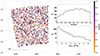 |
Fig. 1. Sky map with the positions of the 2,342 total CosmoDC2 clusters with M200c > 1014 M⊙ that we used for the YOLO-CL training and validation. Larger circle sizes indicate larger masses, and redshift is coded by color, as is indicated in the right bar). In the insert are the dark matter halo redshift and mass distributions. |
For each halo, the catalog includes its position, the true redshift, the dark matter halo mass M200c, and a richness parameter defined as the sum of the probabilities for all galaxies belonging to the halo brighter than m*(z)+2 to be a halo member. Here m* is the characteristic magnitude that corresponds to the luminosity of the knee of the Press–Schechter luminosity function (Press & Schechter 1974) at the redshift of the cluster. To find m*, we fit the galaxy luminosity function in the K band (Lin et al. 2006). Then, we predicted m* in optical bands using the PEGASE2 library (Fioc & Rocca-Volmerange 1999) for a burst galaxy that passively evolves from z = 3. The probability of the galaxy being a cluster member was computed by assigning a weight depending on the projected distance from the cluster center following Rykoff et al. (2012, 2014).
To generate composite color images, we used the DEEPCOADD frames delivered by the LSST pipeline in the DC2 Run2.2 simulation run ((LSST Dark Energy Science Collaboration (LSST DESC) 2021) for the cosmoDC2 v1.1.4 extragalactic catalog (Korytov et al. 2019). These images were fully reduced, calibrated, sky-subtracted, and coadded science frames with a pixel scale of 0.2″/pix. To make our analysis fully consistent with the SDSS images, we resampled the DC2 images to the SDSS pixel scale of 0.39″/pix using the astropy-based REPROJECT package (Robitaille et al. 2020).
To build composite JPEG color images for the DC2 simulation, we used the same algorithm used in the SDSS survey (Lupton et al. 2001). This algorithm has two main parameters: nonlinearity (Q) and flux scale (α). For SDSS, the parameters are Q = 8 and α = 0.29. For the DC2 color images, we used Q = 8 and α = 0.08, in order to partially compensate for the depth and magnitude zeropoint difference (the zero magnitudes are m0SDSS = 22.5 mag and m0LSST = 27 mag). In fact, with α = 0.08, the DC2 scale visually reproduces the SDSS scale. We also adjusted the DC2 flux count range to have a similar range in surface brightness as in SDSS. We performed a sky subtraction, and registered the composite images on a final JPEG scale from 0 to 255. We set to zero and 255 all pixels with fluxes less than zero and larger than 255, respectively.
3. YOLO-CL training and validation
3.1. YOLO-CL
YOLO-CL10 is based on the third iteration of YOLO, YOLOv3 (Redmon & Farhadi 2018), which represents a significant improvement over the first versions, and proved to be very well adapted for cluster detection (Grishin et al. 2023). We outline here the algorithm main characteristics; more details can be found in Grishin et al. (2023). The YOLO architecture applies a single neural network to images, combining object detection and classification into a single process. This results in execution times that are several orders of magnitude faster than those of other detection convolutional networks such as R-CNN (Region Based CNN, Girshick et al. 2013, and the following developments Fast and Faster R-CNN).
The network divides the image into a S × S grid of cells, within which the detection and classification are performed. For each object detection the network predicts B bounding boxes, to which it assigns a set of parameters, including its position, size, the probability of being an object and the probability of belonging to a certain class of objects. The network is trained on a sample of images on which it optimizes the parameters to better detect and classify objects (i.e., it converges on the optimal weights).
During the training process YOLO-CL optimizes a multicomponent loss function ℒ (Redmon et al. 2015; Grishin et al. 2023):
 (1)
(1)
where ℒobj is the “objectness loss” that optimizes the object identification, ℒbbox is the “bounding box loss” that optimizes the bounding box position and size, and ℒclass is the “classification loss” that optimizes the object class. The loss functions quantify the distance between the true parameter values and those estimated by the network. With respect to the original YOLO classification loss function that considers several object classes, in YOLO-CL we removed multiple object classes because we use a single object class: “cluster”. As the bounding box loss, we used the generalized intersection over union (gIoU) loss (Rezatofighi et al. 2019). In fact, the traditional IoU (intersection over union11) metric does not permit us to optimize the corresponding loss term when the true and predicted bounding boxes are nonoverlapping. More details can be found in Grishin et al. (2023).
The YOLO-CL training consists of several iterations, which are called epochs. At each epoch all the images from the training sample are an input for the network which optimizes the network weights and bias that decrease the loss function, making the distance between the true values and those estimated by the network closer. The network is then validated on a validation sample.
The final network output is a catalog of detections with an associated detection probability and the corners of the box that includes the detection (see below). We derived the detection position as the center of this box.
3.2. Training and validation
We used two equal hybrid samples of 12 203 redMaPPer and 1171 DC2 cluster images each for both training and validating YOLO-CL, with the same number but different images for the training and validation. Each of these two samples has an identical redshift and mass distribution, for a total of 24 406 redMaPPer and 2342 DC2 cluster images. Our hybrid training and validation sample approach makes the YOLO-CL learning invariant to the differences in object densities, and all the other differences between SDSS and DC2.
Following Grishin et al. (2023), we started with images of dimension 2048 × 2048 pixels, which corresponds to ∼13.5 × 13.5 arcmin2, which is twice the size of a typical cluster virial radius of 1 Mpc at z ∼ 0.2, and much larger than the typical cluster virial radius at z > 0.5. For the input to the first layer of the network, we resized each image by average pooling to 512 × 512 pixels (with a pixel size equal to eight times the LSST resolution12) and 1024 × 1024 pixels (with a pixel size equal to four times the LSST resolution13), and kept the same stride parameters as in the original YOLOv3 publication; namely, 8, 16, and 32.
These image sizes and stride parameters are a good compromise between keeping high image resolution and our computational power. Our training and validation runs were performed on Centre de Calcul IN2P314 computing cluster, on a NVIDIA Tesla V100-SXM2-32GB GPU, equipped with 32 GB of memory.
Our hyperparameter optimization was performed with respect to memory limits and the stability of the training. Since the weight optimization during the training was done using a gradient descent, the whole process can be a subject to instabilities. There are two main hyper-parameters responsible for the mitigation of these instabilities: the batch size and the learning rate. The size of the training sample is too large to store in memory, and it is not possible to complete the training on the entire sample in one iteration. To overcome this limitation, we split our training sample in subsets (batches) that are processed by the network at the same time. The batch size is limited by two main factors: it cannot be too small, because in this case the derived direction of the gradient would be unstable, and at the same time it cannot be too big, given that memory resources are limited. Due to memory limitations, we used a batch size of 8 for the 512 × 512 images and of 2 for the 1024 × 1024 images.
The other hyper-parameter that is crucial for training is the learning rate. It defines how big the weight variations can be at each epoch. It cannot be too small, otherwise the most optimal weight configuration would never be achieved, and it cannot be too big because it would make the training process less stable. We choose the learning rate varying with the epoch: it starts from a small value, grows up during the first few epochs, called “warm-up” epochs, and after reaching its maximum values asymptotically goes down to the final values (Grishin et al. 2023). Starting, maximal, and final values of the learning rate as well as the number of warm-up epochs are also hyper-parameters and should be defined before the training. We started by setting a learning rate of 10−10, which grows to 10−5 during the first eight warm-up epochs and then slowly decreases to 10−6.
Our input image cutouts were centered on the redMaPPer cluster or DC2 selected dark matter halo positions. This centering should not have an impact on the network learning, which should understand that cluster features should not depend on its position in the image. For this reason, we applied data augmentation, including translation and flipping of a random quantity between zero and half of the image, which change the initial cluster position in the image. This forces the network to focus on the relevant features associated with clusters, independently of their position in the images.
We provide the main parameters of the training configuration in Table 1.
Settings used for the YOLO-CL training.
4. Results
4.1. Network initial detection catalog
We ran YOLO-CL on the training and validation sample for ∼100 epochs. Fig. 2 shows the loss functions for the two samples with different image sizes. In both cases, the training epochs can be split into three parts: (1) the first epochs, in which the weights quickly converge on optimal values due to the large value of the gradient, (2) the search for an optimal loss minimum (epochs 10–40) and (3) the fine-tuning of the solution. In both cases the lowest value of the validation loss function is reached in the first half of the training epochs – for 512 × 512 it is in the range of epochs 10–45, and for 1024 × 1024 it is in the range 10–30.
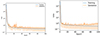 |
Fig. 2. YOLO-CL loss functions for the training (blue) and validation (orange) samples, for the 512 × 512 (left) and 1024 × 1024 (right) images. The vertical bars show the 1σ standard deviation of the validation loss. The training and validation loss functions converge in a smooth way, and their good agreement confirms the network stability in both cases. |
At each epoch, the network output is a catalog of detections on the validation sample, with the bounding box coordinates, and the probability of belonging to the class “cluster” (hereafter detection probability). The network usually outputs multiple detections of the same object, which we discarded by following the standard approach in YOLO applications (Redmon et al. 2015; Redmon & Farhadi 2018). In this case, we defined the IoU as the ratio between the area of intersection and the area of union between multiple detection bounding boxes. The gIoU is an optimization of the IoU (see Sect. 3.1; Rezatofighi et al. 2019), and was defined as
 (2)
(2)
where 𝒰 and 𝒜c are the areas of the union of the two boxes and the smallest box enclosing both boxes, respectively.
Both the IoU and gIoU are a measurement of the overlap region of bounding boxes that define two different detections. A value of 1 indicates perfect agreement (we are detecting the same object), while a value approaching 0 indicates increasingly disjointed boxes and/or significantly different sizes (we are detecting different objects). We discarded multiple detections of the same object by applying a gIoU threshold of 0.5, which is the same threshold as in the original YOLO for the IoU (Rowe et al. 2015; Redmon & Farhadi 2018). This standard choice means that when two bounding boxes overlap more than 50%, we consider that they define the same detected object. In this case, we kept the highest-probability detection while discarding the other.
For each epoch, after discarding multiple detections, we obtained a catalog of single detections, each with the coordinates of the bounding box of the detection and the YOLO-CL probability of the detection being a cluster.
4.2. Final YOLO-CL cluster catalog
At this point, we needed to choose our best epoch and which probability threshold to use to select the best cluster candidates for our final YOLO-CL catalog.
Our best epoch was chosen as the epoch in which the validation loss function reaches its minimum value. This means that in this epoch we reach on average the best values of all the network parameters.
Once we chose the best epoch, to assess our best probability threshold we used two quantities, the final cluster detection catalog completeness and purity, which were calculated on the YOLO-CL DC2 detections with respect to our reference DC2 true cluster sample from the simulation catalog. In fact, while we need a hybrid SDSS and DC2 sample for transfer learning, hereafter all our results will focus on the YOLO-CL performance on DC2 simulations, which are the sample on which we want to test the YOLO-CL performance on LSST, and which define our cluster catalog selection function. For matching true with detected clusters, we used the gIoU criteria described in the previous section.
The cluster catalog completeness quantifies the fraction of true clusters that are detected. The cluster catalog purity quantifies the fraction of detections that are true clusters, as opposed to false positive detections. In ML literature, the completeness corresponds to the recall, and the purity to the precision. To calculate the purity (see below), we applied YOLO-CL to a sample of images (“random” fields) that do not contain DC2 clusters, which means that the center of the random fields is more than 12 arcmin (∼4.5 Mpc at z ≳ 0.5) from any DC2 cluster. For this reason, we added to our validation 6451 random fields, which correspond to all the regions that do not contain clusters in DC2.
We optimized the detection probability threshold to obtain cluster detection catalogs with the highest values of completeness and purity. Following Grishin et al. (2023), we optimized purity and completeness to the same value, so as not to have one variable more optimized with respect to the other. The final YOLO-CL catalog includes only detections that have a detection probability higher than the optimized detection threshold for which completeness and purity are the same. A more fine-tuned selection function can be defined depending on the use of the catalog for cosmology, galaxy formation and evolution studies, and so on.
Figure 3 shows the catalog completeness and purity as a function of the detection probability threshold at our best epoch. The completeness,  , was calculated as the ratio between the number of true cluster detections, Ntd, and the number of true clusters in our images, Ntc. The purity was calculated as
  , where Nrf is the number of random fields and Nfd are cluster detections in the random fields, which are by definition false positive detections. We assume that the ratio
  is a good approximation of the true ratio of false positive detections over the total number of detections, independently of the area of the survey that we considered. The completeness and the purity have the same value of 90% and 94% at the threshold value of 27% and 32% when using the 512 × 512 pixel and 1024 × 1024 pixel images, respectively.
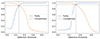 |
Fig. 3. Purity and completeness of the YOLO-CL DC2 detection catalogs for 512 × 512 (left) and 1024 × 1024 (right) images as a function of the detection threshold. The best purity and completeness are 90% and 94% for the 512 × 512 and 1024 × 1024 pixel images, respectively. |
Figure 4 shows the completeness as a function of the DC2 true cluster mass M200c and redshift. The completeness is almost flat at 0.2 < z < 0.8 and varies in the range of 80%–90% and 90%–96% when YOLO-CL is applied to 512 × 512 and 1024 × 1024 pixel images, respectively. At z > 0.8, we observe a decrease in completeness, which is larger when considering 512 × 512 pixel images. The completeness also increases with the halo mass. For the 512 × 512 pixel images the completeness is ≳95% only for halos with M200c > 1014.7 M⊙, while for 1024 × 1024 images it is ≳94% for M200c > 1014 M⊙.
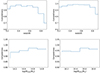 |
Fig. 4. YOLO-CL DC2 detection completeness as a function of redshift (Top), and halo mass M200c (Bottom) for the 512 × 512 (left) and 1024 × 1024 (right) pixel images. The completeness as a function of redshift is almost flat at the region 0.2 < z < 0.8 with an average value of 0.85 for 512 × 512 and 0.95 for 1024 × 1024. |
4.3. YOLO-CL final catalog completeness and purity
Given the higher network performance with 1024 × 1024 pixel images, hereafter we concentrate on the catalog obtained with this image size. In this final YOLO-CL catalog, we have only kept cluster candidates with detection probability higher than a 32% threshold, which corresponds to a catalog that is 94% complete and pure.
Figure 5 shows the YOLO-CL detection catalog completeness as a function of both redshift and DC2 halo mass and richness. Halo mass and richness are correlated, with a large scatter, and a M200c = 1014 M⊙ corresponds to a richness of ∼35. The YOLO-CL selection is almost flat with respect to the halo mass up to z ∼ 0.9, but not with respect to richness. This might be due to the fact that the features found by the network to identify a cluster, or the nonlinear combination of these features, are more closely linked to the cluster mass than to its richness.
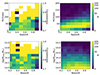 |
Fig. 5. YOLO-CL DC2 detection completeness and the number of halos as a function of redshift and richness or halo mass. Left: YOLO-CL DC2 detection completeness as a function of redshift and richness (top) or halo mass (bottom). Right: Number of halos as a function of redshift and richness (top) or halo mass (bottom). The vertical colored bars show the color scale for the completeness (left) and the number of halos (right). The YOLO-CL selection is almost flat as a function of redshift up to z ∼ 0.8 when we consider the halo mass. The catalog is ∼100% complete for M200c ≳ 1014.6 M⊙ and richness ≳100 at all redshifts. When characterizing halos by their richness, the completeness is less flat as a function of redshift, as is also shown for SDSS observations in Grishin et al. (2023), and the completeness decreases abruptly to ∼70 − 75% at z > 0.8 and M200c ≲ 1014 M⊙. Comparing the figures on the left and on the right, some bins show very low completeness on the left only because there are no clusters in those bins. |
The catalog is ∼100% complete for M200c ≳ 1014.6 M⊙ and richness ≳100 at all redshifts. At M200c ≳ 1014 M⊙, the completeness is ≳95% up to z ∼ 0.8, and decreases to ≳80–85% at higher redshifts. However, when characterizing halos by their richness, the completeness is less flat as a function of redshift, as also shown for SDSS observations in Grishin et al. (2023), and decreases abruptly to ∼70 − 75% at z > 0.8.
To better understand the purity of YOLO-CL catalog as a function of redshift, we matched the 6% false detections to lower-mass DC2 dark matter halos, which are the most probable interlopers. Unfortunately, we cannot estimate purity as a function of both mass and redshift because we would need the number of detected clusters with a given observed mass and redshift, and YOLO-CL does not provide an estimation of these parameters. We found that 49%, 97%, and 100% of the false detections match with halos 1013.8 M⊙ < M200c < 1014 M⊙, 1013.5 M⊙ < M200c < 1014 M⊙, and 1013.4 M⊙ < M200c < 1014 M⊙, respectively, of which 24%, 79%, and 85% are at z < 1, respectively. Fig. 6 shows their distributions as a function of mass and redshift.
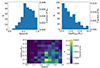 |
Fig. 6. Distribution of the ratio of YOLO-CL DC2 false positive detections to the total number of random fields, Nrf, as a function of halo mass and redshift (Top) and both (Bottom). In the bottom panel, the scale on the right indicates the number of false positive detections, N, and the ratio of N to the total number of random fields, Nrf. The total number of YOLO-CL random fields is 6451. |
Most of the contamination of the final cluster sample is due to groups with 1013.7 M⊙ < M200c < 1014 M⊙ (i.e., objects with masses within 0.3 dex smaller than a cluster) and z ≳ 0.6. From the DES Y1 redMaPPer cluster catalog (McClintock et al. 2019), the cluster mass uncertainty is estimated to be 0.13 dex at z ≲ 1 and M200c > 1014 M⊙ (Farahi et al. 2019). This means that our false positive detections cannot be distinguished from “true clusters” within 3σ of the current DES observational mass uncertainty, which might be taken as a hypothetical lower limit on future LSST cluster mass uncertainties.
The mass observational uncertainty would also introduce an Eddington bias, which means that the more numerous M200c < 1014 M⊙ halos will be assigned a mass estimation of M200c > 1014 M⊙, and then contaminate our cluster sample with lower-mass groups. To estimate this bias, again using the current DES cluster mass uncertainty as a reference, we statistically estimated the number of groups in the DC2 footprint with M200c < 1014 M⊙ that may have a mass estimate of M200c > 1014 M⊙ due to the scatter of the cluster mass-richness relation, and obtained an Eddington bias of 11%.
With this hypothesis, this means that 6% of the detections in the YOLO-CL cluster catalog would be groups with 1013.4 M⊙ < M200c < 1014 M⊙, and at least ∼10% of these groups are expected to be assigned a mass of M200c > 1014 M⊙. In practice, in current surveys the uncertainty on halo mass at M200c < 1014 M⊙ is about two times larger than the uncertainty at M200c < 1014 M⊙, about 0.25–0.3 dex (e.g., Simet et al. 2017; Parroni et al. 2017). If that is also true for LSST, the Eddington bias contamination will be on the order of ∼30%, and all of these estimates have to be reassessed when the LSST cluster mass uncertainties are estimated.
Figure 7 shows the distribution of the angular distance between the true cluster and the YOLO-CL detection center. The average difference is 108 ± 19 kpc. The angular distance distribution is not Gaussian though, and the median is of 112 ± 19 kpc. The angular distance is larger than what we found between cluster centers detected by YOLO-CL and redMaPPer in SDSS (Grishin et al. 2023), but still well within the cluster cores.
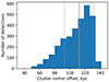 |
Fig. 7. Angular distance between the true cluster and the YOLO-CL detection center (i.e., the center of the YOLO-CL box). |
5. Discussion and conclusions
Our results show that YOLO-CL detects DC2 clusters (M200c > 1014 M⊙) in regions centered around them with ∼94% completeness and purity at 0.2 ≲ z ≲ 1, and with a 100% completeness for M200c > 1014.6 M⊙ within the same redshift range. We also found that the YOLO-CL selection function is almost flat with respect to the halo mass up to z ∼ 0.9. In this section, we discuss how this performance compares with other cluster detection methods in optical imaging surveys and other wavelengths.
At lower redshifts than LSST, the current DES covers 5000 sq. deg. in the g, r, i, z and Y bandpasses and reaches a 10σ depth at 24.7, 24.4 and 23.8 mag in g, r, and i respectively15. This corresponds to a 5σ depth ∼2 mag shallower than LSST. The DES redMaPPer cluster catalog (Rykoff et al. 2016) is 100% complete for a richness of λ > 70, which corresponds to a halo mass of M200c ∼ 1014.8 M⊙, using weak lensing and X-ray halo mass estimations for redMaPPer clusters (McClintock et al. 2019; Upsdell et al. 2023). Given the large difference in survey depth, it is not surprising that this catalog is less complete than YOLO-CL DC2 catalog at lower masses.
When comparing to predictions for cluster catalogs’ completeness and purity at the LSST depth, empirical simulations and a Bayesian cluster finder (Ascaso et al. 2012, 2015) predict a similar completeness and purity as YOLO-CL (86–98%) in the redshift range of 0.5 ≲ z ≲ 1.0 for Mh > 1014.3 M⊙ (Ascaso et al. 2017), which corresponds to M200c > 1014.24 M⊙16.
For observational comparisons, the first survey that reached a depth closer to LSST is the Canada-France-Hawaii Telescope Legacy Survey (CFHT-LS)17 (Gwyn 2012). The median 50% completeness limits in its four deep fields (∼4 sq. deg.) are 26.3, 26.3 and 25.9 in the g, r, and i bandpasses, respectively (Cabanac et al. 2007). When we analyzed the 5σ limit, we obtained similar depths as LSST in these three bands. Several algorithms were applied to the CFHT-LS deep fields to obtain galaxy cluster samples 90–95% complete at 0.2 < z < 0.8 and 90% pure for clusters with a richness of λ > 50 in simulated data (Grove et al. 2009), and 100% complete and 85–90% pure at M200c > 1014.5 M⊙ (Milkeraitis et al. 2010).
A recent survey that reaches a depth similar to LSST and uses similar optical filters is the Hyper Suprime Camera Strategic Survey Program (HSC-SSP; Aihara et al. 2018), which covers an area of ∼1000 sq. deg. and reaches a 5σ depth of 26.8 mag and 26.4 mag in the g and i bandpasses, respectively. The HSC-SSP cluster catalog obtained with the CAMIRA algorithm (Oguri 2014) is 100% and ∼90% complete and ≳90% pure for M200c > 1014.64 M⊙ and M200c > 1013.94 M⊙, respectively, in the redshift range 0.1 ≲ z ≲ 1.1 (Oguri et al. 2018). The CAMIRA algorithm is similar to redMaPPer, and searches for red-sequence galaxy overdensities. The WHL09/12 algorithm (Wen et al. 2009, 2012), applied to a compilation of the HSC-SSP and unWISE catalogs, delivers a cluster catalog that is 100% complete for M200c > 1014.8 M⊙ (Wen & Han 2021), and 80–90% complete for M200c > 1014.4 M⊙ at 0.2 ≲ z ≲ 1. The purity of the sample is not discussed. The completeness significantly decreases for lower cluster mass, reaching ≲70–60% completeness for M200c > 1014.1 M⊙.
When compared to the completeness and purity expected for Euclid cluster catalogs at z < 1 (Euclid Collaboration: Adam et al. 2019) using simulations from Ascaso et al. (2015), the YOLO-CL DC2 detections are more complete and pure for M > 1014 M⊙. The best purity and completeness of ∼90% at this mass and redshift range were obtained with the algorithm AMICO (Bellagamba et al. 2018). The other Euclid cluster finder, PZWav, based on wavelet filtering, gives catalogs that are ∼85–87% complete and pure (Euclid Collaboration: Adam et al. 2019).
Overall, the performance of YOLO-CL on DC2 simulations is similar to or higher than both current optical surveys at the same depth and redshift range, and LSST and Euclid simulation predictions for future cluster catalogs.
To compare with present and future cluster catalogs obtained at other wavelengths, we compared our results with cluster catalogs obtained by the Sunyaev–Zeldovich (SZ; Sunyaev & Zeldovich 1972) effect and X-ray flux measurements, which are both sensitive to the cluster hot gas content.
SZ cluster catalogs are mass-limited and the deepest catalogs available at present reach 100% completeness at M200c > 1014.86 − 1014.94 M⊙ at z ≲ 1.5 from observations with the South Pole Telescope Polarimeter (SPTPol; Bleem et al. 2020), a much higher mass limit than optical and infrared surveys have. The SPT-SZ survey (Bleem et al. 2015) catalog is 100% complete at M200c > 1014.94 − 1015.00 M⊙ in a similar redshift range. The cluster catalog obtained from the fifth data release (DR5) of observations (13 211 deg2) with the Atacama Cosmology Telescope (ACT) is 90% complete for the clusters with M200c > 1014.76 − 14.66 at 0.2 < z < 2.0 (Hilton et al. 2021). The Planck space mission PSZ2 all-sky cluster catalog (Planck Collaboration XXVII 2016) is 80% complete for M200c > 1014.76 M⊙ at 0.4 < z < 0.6, and for M200c > 1014.3 M⊙ for clusters at z ∼ 0.2.
Simulations of the current SPT-3G survey, which will provide much deeper observations (Benson et al. 2014), were used to estimate the completeness and purity that can be attained with another deep CNN (Lin et al. 2021), combined with a classical match filter (Melin et al. 2006). This work shows that ∼95% completeness and purity is predicted to be attained at M200c > 1014.7 M⊙ at z ≳ 0.25.
This means that all present SZ surveys reach ∼95% completeness at cluster masses much higher than what is predicted for LSST from this work. However, the next-generation SZ experiments such as SPT-3G, Simons Observatory, and CMB-S4 will obtain cluster catalogs with a limiting mass M200c ∼ 1014 M⊙ which is more comparable to the LSST mass limit (Raghunathan 2022). The CMB-S4 WIDE (Abazajian et al. 2016) survey will reach the S/N = 5 cluster detection limit of M200c = 1014.1 M⊙ at the redshift range 0.2 < z < 1 over 67% of the sky; the S/N = 5 detection threshold for the Simons Observatory (Ade et al. 2019) is planned to be M200c = 1014.3 M⊙ in the same redshift range over 40% of the sky; and the CMB-S4 ULTRADEEP and CMB-HD (Sehgal et al. 2019) surveys are built to reach up to M200c = 1014 M⊙ and M200c = 1013.8 M⊙, respectively. However, the CMB-S4 ULTRADEEP survey covers only 3% of the sky, while CMB-HD is planned to cover ∼50% of the sky. All of these survey are planned for ≳2030, most probably at about the same time as the 5-year LSST data release.
For X-ray surveys, the reference X-ray all-sky cluster catalog is the Röntgensatellit (ROSAT; Pfeffermann et al. 1987; Voges et al. 1999) catalog of Extended Brightest Cluster Sample (BCS; Ebeling et al. 1998), which contains 201 cluster in the northern hemisphere and which is 90% complete for z < 0.3 and X-ray fluxes higher than 4.4 ⋅ 10−12 erg/cm2/s. The MCXC cluster catalog (Piffaretti et al. 2011) is a compilation of several catalogs and surveys that consists of ROSAT-based catalogs and serendipitous catalogs, summarized in Table A.1. As was expected, X-ray surveys detect clusters at much higher masses than LSST at z = 0.5–1.
The ComPRASS catalog (Tarrío et al. 2019) presents a compilation of Planck (Planck Collaboration XXVII 2016) and RASS (Popesso et al. 2004) catalogs of galaxy clusters that were observed in X-ray and using SZ, and reaches deeper than each survey used to compile it. Therefore, the selection function is a complicated combination of the selection function of several surveys. CompRASS is 100% complete for M200c > 1014.6 M⊙, M200c > 1014.8 M⊙, and M200c > 1014.7 M⊙ at z < 0.3, z < 0.6, and 0.6 < z < 1.0, respectively, which are much lower than the completeness limit for the SZ catalogs used to build it.
In conclusion, YOLO-CL shows a similar completeness and purity to other algorithms applied to current deep optical imaging surveys such as CFHTLS Deep and HSC-SSP, and a better completeness and purity than most of the other methods that have been applied to Euclid simulations. Compared to current SZ and X-ray surveys, YOLO-CL can obtain more complete and pure catalogs at much lower masses. However, future SZ surveys are planned to provide much deeper catalogs whose completeness and purity are estimated to be directly comparable with ours. With respect to this, we notice that both SZ surveys and the YOLO-CL selection function are mass-limited, making the SZ-optical comparison be also based on similar selection functions. YOLO-CL detections can also be combined with SZ and X-ray detections as was done for the ComPRASS compilation, to reach catalogs with higher completeness and purity at lower masses.
It has to be noted that in this paper we have focused our analysis on the targeted detections, with the goal being to analyze the performance of the algorithm itself, independently of possible systematics and biases introduced by variations in the parameters of the images generated in a survey mode. In future papers, we shall apply YOLO-CL to DC2 images in a survey mode, and our detections will be compared to other LSST cluster detection algorithms applied to the DC2 simulations.
6. Summary
We applied the YOLO-CL deep convolutional network (Grishin et al. 2023) to observations from SDSS and DESC DC2 simulations to estimate its performance for LSST. We trained the network on 12 203 and 1171 g, r, and i composite color images from SDSS and from the DESC DC2 simulations, respectively, and validated it on the same number of cluster images (for a total of 24 406 SDSS and 2342 DC2 training and validation images) and 6451 random fields. We conclude that:
-
When using DC2 LSST simulated images with a pixel size equal to four times the LSST pixel resolution (≈0.8″/pix), the YOLO-CL DC2 cluster catalog is 94% pure and complete for M200c > 1014 M⊙ and at 0.2 < z < 1, and 100% complete for M200c > 1014.6 M⊙.
-
The cluster selection function is mass-limited at 0.2 < z < 0.9.
-
When compared to other cluster detection methods in current optical surveys that reach the LSST depth and simulations of the Euclid surveys, YOLO-CL shows a similar or better completeness and purity.
-
Current X-ray and SZ cluster surveys do not reach YOLO-CL completeness and purity at M200c > 1014 M⊙ and at 0.2 < z < 1, while future SZ surveys will be directly comparable to LSST YOLO-CL detections and will have similar mass-limited selection functions.
This paper shows that YOLO-CL will permit us to obtain LSST cluster catalogs that will be 94% pure and complete for M200c > 1014 M⊙ and at 0.2 < z < 1, and 100% for M200c > 1014.6 M⊙ The YOLO-CL cluster selection function is mass-limited in the redshift range 0.2 < z < 0.9. We focused our analysis on targeted detections, with the goal of analyzing the performance of the algorithm itself, independently of possible systematics and biases introduced by a survey mode.
We have compared our algorithm to other cluster detection methods in current optical surveys that reach LSST depth and simulations of the Euclid surveys, and YOLO-CL shows a similar or better completeness and purity. When compared to current X-ray and SZ cluster surveys YOLO-CL reaches a higher completeness and purity at M200c > 1014 M⊙ and at 0.2 < z < 1. However, future SZ surveys will reach a similar completeness and purity at the same depth as LSST YOLO-CL detections, and will have similar mass-limited selection functions.
We note that this analysis was based on LSST DC2 images and did not involve the image processing required to obtain galaxy photometric and photometric redshift catalogs, or the masking of stellar sources and artifacts. The advantage of this deep ML approach that works directly on images is that it obtains cluster catalogs that will be complementary to other optical detection methods used in the LSST DESC collaboration, and that will be independent from systematic and statistical uncertainties inherent to galaxy catalog production.
In future papers, we shall study the YOLO-CL performance in survey mode, and our detections will be compared to other LSST cluster detection algorithms.
Version 6.3 of the catalog, from the VizieR archive: https://vizier.cds.unistra.fr
By definition, the cluster richness is the number of cluster members above a given luminosity. For redMaPPer it is defined as a sum of the probability of being a cluster member over all galaxies in a cluster field (Rozo et al. 2009).
Detailed here: https://www.sdss.org/dr16/imaging/jpg-images-on-skyserver
M200c is defined as the mass within the circular region of radius R200 containing a mean mass density equal to two hundred times the critical density of the Universe at a given redshift.
GITHUB PAGE.
The IoU is defined as the ratio between the area of intersection and the area of union between the detected object bounding box and the “true object” bounding box (Redmon et al. 2015).
Four times the SDSS resolution.
The double of the SDSS resolution.
Hereafter, M200c masses were derived from the original Mh and M500 masses found in the literature, using the web calculator for the equations from Ragagnin et al. (2021), https://c2papcosmosim.uc.lrz.de/static/hydro_mc/webapp/index.html
Acknowledgments
We thank Université Paris Cité (UPC), which founded KG’s Ph.D. research. We gratefully acknowledge support from the CNRS/IN2P3 Computing Center (Lyon - France) for providing computing and data-processing resources needed for this work. We describe below the author’s contributions. Kirill Grishin applied YOLO-CL to the DC2 simulations, produced the results and figures in the paper, and was the main writer of Sections 2.2 and 5. Simona Mei co-conceived the YOLO-CL network with Stéphane Ilic, developed the content of this paper, supervised the work of Kirill Grishin, Stéphane Ilic and Michel Aguena, and was the main writer of the paper’s text, answered the internal DESC reports, answered the A&A referee report and edited the paper as the main contact with the editor. Stéphane Ilic modified the original YOLO network to adapt it for galaxy cluster detection. He co-conceived YOLO-CL with Simona Mei and developed the network and analysis software to derive the completeness and purity plots. Michel Aguena contributed to the generation and validation of the DC2 images, and to the analysis and discussion of the cluster detection, including the improvement on the purity estimation model. He also shaped the final image generation software used, and provided the masses and richnesses estimations to the dark matter halo catalog. Dominique Boutigny and Marie Paturel helped with image generation at the beginning of the project and experimented with different versions of YOLO. These statements have been validated with the DESC publication board after having the confirmation of the authors. The Dark Energy Science Collaboration (DESC) acknowledges ongoing support from the IN2P3 (France), the STFC (United Kingdom), and the DOE, NSF, and LSST Corporation (United States). As members of the DESC collaboration, we used resources of the IN2P3 Computing Center (CC-IN2P3–Lyon/Villeurbanne – France) funded by the Centre National de la Recherche Scientifique; the National Energy Research Scientific Computing Center, a DOE Office of Science User Facility supported under Contract No. DE-AC02-05CH11231; STFC DiRAC HPC Facilities, funded by UK BEIS National E-infrastructure capital grants; and the UK particle physics grid, supported by the GridPP Collaboration. This work was performed in part under DOE Contract DE-AC02-76SF00515. This work was supported by CNES, focused on the Euclid space mission. This paper has undergone an internal review by the LSST DESC, and we thank the internal reviewers, Camille Avestruz and Markus Michael Rau, for fruitful discussions that improved the paper. We thank the anonymous referee for very useful suggestions that also improved the paper.
References
- Abazajian, K. N., Adelman-McCarthy, J. K., Agüeros, M. A., et al. 2009, ApJS, 182, 543 [Google Scholar]
- Abazajian, K. N., Adshead, P., Ahmed, Z., et al. 2016, arXiv e-prints [arXiv:1610.02743] [Google Scholar]
- Abbott, T. M. C., Abdalla, F. B., Allam, S., et al. 2018, ApJS, 239, 18 [Google Scholar]
- Ade, P., Aguirre, J., Ahmed, Z., et al. 2019, JCAP, 2019, 056 [Google Scholar]
- Aihara, H., Armstrong, R., Bickerton, S., et al. 2018, PASJ, 70, S8 [NASA ADS] [Google Scholar]
- Angora, G., Rosati, P., Meneghetti, M., et al. 2023, A&A, 676, A40 [NASA ADS] [CrossRef] [EDP Sciences] [Google Scholar]
- Ascaso, B., Wittman, D., & Benítez, N. 2012, MNRAS, 420, 1167 [NASA ADS] [CrossRef] [Google Scholar]
- Ascaso, B., Mei, S., & Benítez, N. 2015, MNRAS, 453, 2515 [Google Scholar]
- Ascaso, B., Mei, S., Bartlett, J. G., & Benítez, N. 2017, MNRAS, 464, 2270 [CrossRef] [Google Scholar]
- Bayliss, M. B., Hennawi, J. F., Gladders, M. D., et al. 2011, ApJS, 193, 8 [Google Scholar]
- Behroozi, P., Wechsler, R. H., Hearin, A. P., & Conroy, C. 2019, MNRAS, 488, 3143 [NASA ADS] [CrossRef] [Google Scholar]
- Bellagamba, F., Roncarelli, M., Maturi, M., & Moscardini, L. 2018, MNRAS, 473, 5221 [NASA ADS] [CrossRef] [Google Scholar]
- Benson, A. J. 2012, New A, 17, 175 [NASA ADS] [CrossRef] [Google Scholar]
- Benson, B. A., Ade, P. A. R., Ahmed, Z., et al. 2014, in Millimeter, Submillimeter, and Far-Infrared Detectors and Instrumentation for Astronomy VII, eds. W. S. Holland, & J. Zmuidzinas, SPIE Conf. Ser., 9153, 91531P [NASA ADS] [CrossRef] [Google Scholar]
- Bleem, L. E., Stalder, B., de Haan, T., et al. 2015, ApJS, 216, 27 [Google Scholar]
- Bleem, L. E., Bocquet, S., Stalder, B., et al. 2020, ApJS, 247, 25 [Google Scholar]
- Bohringer, H., Voges, W., Huchra, J. P., et al. 2000, ApJS, 129, 435 [CrossRef] [Google Scholar]
- Bohringer, H., Schuecker, P., Guzzo, L., et al. 2004, A&A, 425, 367 [NASA ADS] [CrossRef] [EDP Sciences] [Google Scholar]
- Bonjean, V. 2020, A&A, 634, A81 [NASA ADS] [CrossRef] [EDP Sciences] [Google Scholar]
- Bosch, J., Armstrong, R., Bickerton, S., et al. 2018, PASJ, 70, S5 [Google Scholar]
- Brunner, H., Liu, T., Lamer, G., et al. 2022, A&A, 661, A1 [NASA ADS] [CrossRef] [EDP Sciences] [Google Scholar]
- Bruzual, G., & Charlot, S. 2003, MNRAS, 344, 1000 [NASA ADS] [CrossRef] [Google Scholar]
- Burenin, R. A., Vikhlinin, A., Hornstrup, A., et al. 2007, ApJS, 172, 561 [Google Scholar]
- Burke, D. J., Collins, C. A., Sharples, R. M., Romer, A. K., & Nichol, R. C. 2003, MNRAS, 341, 1093 [NASA ADS] [CrossRef] [Google Scholar]
- Cabanac, R. A., Alard, C., Dantel-Fort, M., et al. 2007, A&A, 461, 813 [NASA ADS] [CrossRef] [EDP Sciences] [Google Scholar]
- Chan, M. C., & Stott, J. P. 2019, MNRAS, 490, 5770 [NASA ADS] [CrossRef] [Google Scholar]
- Chen, X., Zhu, F., Gaines, S., & Padmanabhan, N. 2023, MNRAS, 523, 6272 [NASA ADS] [CrossRef] [Google Scholar]
- Cornu, D., & Montillaud, J. 2021, A&A, 647, A116 [NASA ADS] [CrossRef] [EDP Sciences] [Google Scholar]
- Cornu, D., Salomé, P., Semelin, B., et al. 2024, A&A, 690, A211 [NASA ADS] [CrossRef] [EDP Sciences] [Google Scholar]
- Cruddace, R., Voges, W., Böhringer, H., et al. 2002, ApJS, 140, 239 [NASA ADS] [CrossRef] [Google Scholar]
- Davidzon, I., Jegatheesan, K., Ilbert, O., et al. 2022, A&A, 665, A34 [NASA ADS] [CrossRef] [EDP Sciences] [Google Scholar]
- Dimauro, P., Huertas-Company, M., Daddi, E., et al. 2018, MNRAS, 478, 5410 [Google Scholar]
- Domínguez Sánchez, H., Huertas-Company, M., Bernardi, M., Tuccillo, D., & Fischer, J. L. 2018, MNRAS, 476, 3661 [Google Scholar]
- Ebeling, H., Edge, A. C., Bohringer, H., et al. 1998, MNRAS, 301, 881 [Google Scholar]
- Ebeling, H., Edge, A. C., & Henry, J. P. 2001, ApJ, 553, 668 [Google Scholar]
- Eifler, T., Miyatake, H., Krause, E., et al. 2021, MNRAS, 507, 1746 [NASA ADS] [CrossRef] [Google Scholar]
- Euclid Collaboration (Adam, R., et al.) 2019, A&A, 627, A23 [NASA ADS] [CrossRef] [EDP Sciences] [Google Scholar]
- Euclid Collaboration (Bretonnière, H., et al.) 2022, A&A, 657, A90 [CrossRef] [EDP Sciences] [Google Scholar]
- Euclid Collaboration (Bisigello, L., et al.) 2023a, MNRAS, 520, 3529 [NASA ADS] [CrossRef] [Google Scholar]
- Euclid Collaboration (Humphrey, A., et al.) 2023b, A&A, 671, A99 [NASA ADS] [CrossRef] [EDP Sciences] [Google Scholar]
- Evrard, A. E., Bialek, J., Busha, M., et al. 2008, ApJ, 672, 122 [Google Scholar]
- Farahi, A., Chen, X., Evrard, A. E., et al. 2019, MNRAS, 490, 3341 [NASA ADS] [CrossRef] [Google Scholar]
- Fioc, M., & Rocca-Volmerange, B. 1999, arXiv e-prints [arXiv:astro-ph/9912179] [Google Scholar]
- Gioia, I. M., Henry, J. P., Maccacaro, T., et al. 1990, ApJ, 356, L35 [NASA ADS] [CrossRef] [Google Scholar]
- Girshick, R., Donahue, J., Darrell, T., & Malik, J. 2013, arXiv e-prints [arXiv:1311.2524] [Google Scholar]
- Gladders, M. D., & Yee, H. K. C. 2005, ApJS, 157, 1 [NASA ADS] [CrossRef] [Google Scholar]
- Górski, K. M., Hivon, E., Banday, A. J., et al. 2005, ApJ, 622, 759 [Google Scholar]
- Grishin, K., Mei, S., & Ilić, S. 2023, A&A, 677, A101 [NASA ADS] [CrossRef] [EDP Sciences] [Google Scholar]
- Grove, L. F., Benoist, C., & Martel, F. 2009, A&A, 494, 845 [NASA ADS] [CrossRef] [EDP Sciences] [Google Scholar]
- Gwyn, S. D. J. 2012, AJ, 143, 38 [Google Scholar]
- Hao, J., McKay, T. A., Koester, B. P., et al. 2010, ApJS, 191, 254 [Google Scholar]
- Heitmann, K., Finkel, H., Pope, A., et al. 2019, ApJS, 245, 16 [NASA ADS] [CrossRef] [Google Scholar]
- Henghes, B., Pettitt, C., Thiyagalingam, J., Hey, T., & Lahav, O. 2021, MNRAS, 505, 4847 [CrossRef] [Google Scholar]
- Henry, J. P., Mullis, C. R., Voges, W., et al. 2006, ApJS, 162, 304 [NASA ADS] [CrossRef] [Google Scholar]
- Hezaveh, Y. D., Perreault Levasseur, L., & Marshall, P. J. 2017, Nature, 548, 555 [Google Scholar]
- Hilton, M., Sifón, C., Naess, S., et al. 2021, ApJS, 253, 3 [Google Scholar]
- Horner, D. J., Perlman, E. S., Ebeling, H., et al. 2008, ApJS, 176, 374 [NASA ADS] [CrossRef] [Google Scholar]
- Huertas-Company, M., & Lanusse, F. 2023, PASA, 40, e001 [NASA ADS] [CrossRef] [Google Scholar]
- Huertas-Company, M., Gravet, R., Cabrera-Vives, G., et al. 2015, ApJS, 221, 8 [NASA ADS] [CrossRef] [Google Scholar]
- Huertas-Company, M., Primack, J. R., Dekel, A., et al. 2018, ApJ, 858, 114 [NASA ADS] [CrossRef] [Google Scholar]
- Hurier, G., Aghanim, N., & Douspis, M. 2021, A&A, 653, A106 [NASA ADS] [CrossRef] [EDP Sciences] [Google Scholar]
- Ivezić, Ž., & the LSST Science Collaboration 2013, LSST Science Requirements Document, http://ls.st/LPM-17 [Google Scholar]
- Ivezić, Ž., Kahn, S. M., Tyson, J. A., et al. 2019, ApJ, 873, 111 [Google Scholar]
- Jeffrey, N., Lanusse, F., Lahav, O., & Starck, J.-L. 2020, MNRAS, 492, 5023 [Google Scholar]
- Kahn, S. 2018, in 42nd COSPAR Scientific Assembly, 42, E1.16-5-18 [Google Scholar]
- Kluge, M., Comparat, J., Liu, A., et al. 2024, A&A, 688, A210 [NASA ADS] [CrossRef] [EDP Sciences] [Google Scholar]
- Knobel, C., Lilly, S. J., Iovino, A., et al. 2009, ApJ, 697, 1842 [NASA ADS] [CrossRef] [Google Scholar]
- Koester, B. P., McKay, T. A., Annis, J., et al. 2007, ApJ, 660, 239 [NASA ADS] [CrossRef] [Google Scholar]
- Korytov, D., Hearin, A., Kovacs, E., et al. 2019, ApJS, 245, 26 [NASA ADS] [CrossRef] [Google Scholar]
- Kovacs, E., Mao, Y.-Y., Aguena, M., et al. 2022, Open J. Astrophys., 5, 1 [NASA ADS] [CrossRef] [Google Scholar]
- Laureijs, R., Amiaux, J., Arduini, S., et al. 2011, arXiv e-prints [arXiv:1110.3193] [Google Scholar]
- Licitra, R., Mei, S., Raichoor, A., Erben, T., & Hildebrandt, H. 2016a, MNRAS, 455, 3020 [NASA ADS] [CrossRef] [Google Scholar]
- Licitra, R., Mei, S., Raichoor, A., et al. 2016b, ApJ, 829, 44 [CrossRef] [Google Scholar]
- Lin, Y.-T., Mohr, J. J., Gonzalez, A. H., & Stanford, S. A. 2006, ApJ, 650, L99 [Google Scholar]
- Lin, Z., Huang, N., Avestruz, C., et al. 2021, MNRAS, 507, 4149 [NASA ADS] [CrossRef] [Google Scholar]
- LSST Dark Energy Science Collaboration (LSST DESC) (Abolfathi, B., et al.) 2021, ApJS, 253, 31 [CrossRef] [Google Scholar]
- LSST Science Collaboration (Abell, P. A., et al.) 2009, arXiv e-prints [arXiv:0912.0201] [Google Scholar]
- Lupton, R., Gunn, J. E., Ivezić, Z., & Knapp, G. R. 2001, in Astronomical Data Analysis Software and Systems X, eds. J. Harnden, F. R. Harnden, F. A. Primini, & H. E. Payne, ASP Conf. Ser., 238, 269 [NASA ADS] [Google Scholar]
- Lupton, R., Blanton, M. R., Fekete, G., et al. 2004, PASP, 116, 133 [NASA ADS] [CrossRef] [Google Scholar]
- Mao, Y.-Y., Kovacs, E., Heitmann, K., et al. 2018, ApJS, 234, 36 [NASA ADS] [Google Scholar]
- Maturi, M., Bellagamba, F., Radovich, M., et al. 2019, MNRAS, 485, 498 [Google Scholar]
- McClintock, T., Varga, T. N., Gruen, D., et al. 2019, MNRAS, 482, 1352 [Google Scholar]
- Mei, S., Scarlata, C., Pentericci, L., et al. 2015, ApJ, 804, 117 [NASA ADS] [CrossRef] [Google Scholar]
- Melchior, P., Sheldon, E., Drlica-Wagner, A., et al. 2016, Astron. Comput., 16, 99 [NASA ADS] [Google Scholar]
- Melin, J. B., Bartlett, J. G., & Delabrouille, J. 2006, A&A, 459, 341 [NASA ADS] [CrossRef] [EDP Sciences] [Google Scholar]
- Merloni, A., Lamer, G., Liu, T., et al. 2024, A&A, 682, A34 [NASA ADS] [CrossRef] [EDP Sciences] [Google Scholar]
- Milkeraitis, M., van Waerbeke, L., Heymans, C., et al. 2010, MNRAS, 406, 673 [CrossRef] [Google Scholar]
- Moskowitz, I., Gawiser, E., Crenshaw, J. F., et al. 2024, ApJ, 967, L6 [Google Scholar]
- Mullis, C. R., McNamara, B. R., Quintana, H., et al. 2003, ApJ, 594, 154 [NASA ADS] [CrossRef] [Google Scholar]
- Muzzin, A., Wilson, G., Yee, H. K. C., et al. 2012, ApJ, 746, 188 [Google Scholar]
- Oguri, M. 2014, MNRAS, 444, 147 [NASA ADS] [CrossRef] [Google Scholar]
- Oguri, M., Lin, Y.-T., Lin, S.-C., et al. 2018, PASJ, 70, S20 [NASA ADS] [Google Scholar]
- Oke, J. B., & Gunn, J. E. 1983, ApJ, 266, 713 [NASA ADS] [CrossRef] [Google Scholar]
- Olivier, S. S., Seppala, L., Gilmore, K., Hale, L., & Whistler, W. 2006, SPIE Conf. Ser., 6273, 62730Y [NASA ADS] [Google Scholar]
- Olivier, S. S., Riot, V. J., Gilmore, D. K., et al. 2012, in Ground-based and Airborne Instrumentation for Astronomy IV, eds. I. S. McLean, S. K. Ramsay, & H. Takami, SPIE Conf. Ser., 8446, 84466B [Google Scholar]
- Parroni, C., Mei, S., Erben, T., et al. 2017, ApJ, 848, 114 [Google Scholar]
- Pasquet, J., Bertin, E., Treyer, M., Arnouts, S., & Fouchez, D. 2019, A&A, 621, A26 [NASA ADS] [CrossRef] [EDP Sciences] [Google Scholar]
- Perlman, E. S., Horner, D. J., Jones, L. R., et al. 2002, ApJS, 140, 265 [NASA ADS] [CrossRef] [Google Scholar]
- Pfeffermann, E., Briel, U. G., Hippmann, H., et al. 1987, in Soft X-ray optics and technology, eds. E. Koch, & G. A. Schmahl, SPIE Conf. Ser., 733, 519 [NASA ADS] [Google Scholar]
- Piffaretti, R., Arnaud, M., Pratt, G. W., Pointecouteau, E., & Melin, J. B. 2011, A&A, 534, A109 [NASA ADS] [CrossRef] [EDP Sciences] [Google Scholar]
- Planck Collaboration XXVII. 2016, A&A, 594, A27 [NASA ADS] [CrossRef] [EDP Sciences] [Google Scholar]
- Popesso, P., Böhringer, H., Brinkmann, J., Voges, W., & York, D. G. 2004, A&A, 423, 449 [NASA ADS] [CrossRef] [EDP Sciences] [Google Scholar]
- Pratt, G. W., Croston, J. H., Arnaud, M., & Böhringer, H. 2009, A&A, 498, 361 [NASA ADS] [CrossRef] [EDP Sciences] [Google Scholar]
- Press, W. H., & Schechter, P. 1974, ApJ, 187, 425 [Google Scholar]
- Ragagnin, A., Saro, A., Singh, P., & Dolag, K. 2021, MNRAS, 500, 5056 [Google Scholar]
- Raghunathan, S. 2022, ApJ, 928, 16 [NASA ADS] [CrossRef] [Google Scholar]
- Redmon, J., & Farhadi, A. 2016, arXiv e-prints [arXiv:1612.08242] [Google Scholar]
- Redmon, J., & Farhadi, A. 2018, arXiv e-prints [arXiv:1804.02767] [Google Scholar]
- Redmon, J., Divvala, S., Girshick, R., & Farhadi, A. 2015, arXiv e-prints [arXiv:1506.02640] [Google Scholar]
- Rezatofighi, H., Tsoi, N., Gwak, J., et al. 2019, Proceedings of the IEEE/CVF Conference on Computer Vision and Pattern Recognition (CVPR), 658 [Google Scholar]
- Robitaille, T., Deil, C., & Ginsburg, A. 2020, reproject: Python-based astronomical image reprojection, Astrophysics Source Code Library [record ascl:2011.023] [Google Scholar]
- Romer, A. K., Nichol, R. C., Holden, B. P., et al. 2000, ApJS, 126, 209 [NASA ADS] [CrossRef] [Google Scholar]
- Roodman, A., Bogart, J. R., Bond, T., et al. 2018, in Modeling, Systems Engineering, and Project Management for Astronomy VIII, eds. G. Z. Angeli, & P. Dierickx, SPIE Conf. Ser., 10705, 107050D [NASA ADS] [Google Scholar]
- Rowe, B. T. P., Jarvis, M., Mandelbaum, R., et al. 2015, Astron. Comput., 10, 121 [Google Scholar]
- Rozo, E., Rykoff, E. S., Koester, B. P., et al. 2009, ApJ, 703, 601 [NASA ADS] [CrossRef] [Google Scholar]
- Rykoff, E. S., Koester, B. P., Rozo, E., et al. 2012, ApJ, 746, 178 [NASA ADS] [CrossRef] [Google Scholar]
- Rykoff, E. S., Rozo, E., Busha, M. T., et al. 2014, ApJ, 785, 104 [Google Scholar]
- Rykoff, E. S., Rozo, E., Hollowood, D., et al. 2016, ApJS, 224, 1 [NASA ADS] [CrossRef] [Google Scholar]
- Sehgal, N., Aiola, S., Akrami, Y., et al. 2019, BAAS, 51, 6 [NASA ADS] [Google Scholar]
- Simet, M., McClintock, T., Mandelbaum, R., et al. 2017, MNRAS, 466, 3103 [NASA ADS] [CrossRef] [Google Scholar]
- Sirianni, M., Jee, M. J., Benítez, N., et al. 2005, PASP, 117, 1049 [Google Scholar]
- Sobral, D., Best, P. N., Geach, J. E., et al. 2010, MNRAS, 404, 1551 [NASA ADS] [Google Scholar]
- Sunyaev, R. A., & Zeldovich, Y. B. 1972, Comm. Astrophys. Space Phys., 4, 173 [Google Scholar]
- Szabo, T., Pierpaoli, E., Dong, F., Pipino, A., & Gunn, J. 2011, ApJ, 736, 21 [NASA ADS] [CrossRef] [Google Scholar]
- Tarrío, P., Melin, J. B., & Arnaud, M. 2019, A&A, 626, A7 [NASA ADS] [CrossRef] [EDP Sciences] [Google Scholar]
- The LSST Dark Energy Science Collaboration (Mandelbaum, R., et al.) 2018, arXiv e-prints [arXiv:1809.01669] [Google Scholar]
- Upsdell, E. W., Giles, P. A., Romer, A. K., et al. 2023, MNRAS, 522, 5267 [NASA ADS] [CrossRef] [Google Scholar]
- Voges, W., Aschenbach, B., Boller, T., et al. 1999, A&A, 349, 389 [NASA ADS] [Google Scholar]
- Wen, Z. L., & Han, J. L. 2021, MNRAS, 500, 1003 [Google Scholar]
- Wen, Z. L., Han, J. L., & Liu, F. S. 2009, ApJS, 183, 197 [NASA ADS] [CrossRef] [Google Scholar]
- Wen, Z. L., Han, J. L., & Liu, F. S. 2012, ApJS, 199, 34 [Google Scholar]
- Werner, S. V., Cypriano, E. S., Gonzalez, A. H., et al. 2023, MNRAS, 519, 2630 [Google Scholar]
- Wylezalek, D., Galametz, A., Stern, D., et al. 2013, ApJ, 769, 79 [NASA ADS] [CrossRef] [Google Scholar]
- Wylezalek, D., Vernet, J., De Breuck, C., et al. 2014, ApJ, 786, 17 [NASA ADS] [CrossRef] [Google Scholar]
- Yoachim, P., Coughlin, M., Angeli, G. Z., et al. 2016, in Observatory Operations: Strategies, Processes, and Systems VI, eds. A. B. Peck, R. L. Seaman, & C. R. Benn, SPIE Conf. Ser., 9910, 99101A [Google Scholar]
- York, D. G., Adelman, J., Anderson, J. E., Jr, et al. 2000, AJ, 120, 1579 [Google Scholar]
- Zanisi, L., Huertas-Company, M., Lanusse, F., et al. 2021, MNRAS, 501, 4359 [NASA ADS] [CrossRef] [Google Scholar]
Appendix A: Additional table
Completeness of X-ray cluster catalogs. Columns are: 1. Full name of the catalog, 2. Acronym of the catalog, 3. Percentage of the total sky area observed by the survey, 4. Redshift range, 5. Limiting observed flux FX, 6. Completeness for flux > FX, and 7. M200c mass limit at the median redshift, and at z=0.5-1, calculated following Pratt et al. (2009). We indicate the redshift (or the redshift range) in parenthesis.
All Tables
Completeness of X-ray cluster catalogs. Columns are: 1. Full name of the catalog, 2. Acronym of the catalog, 3. Percentage of the total sky area observed by the survey, 4. Redshift range, 5. Limiting observed flux FX, 6. Completeness for flux > FX, and 7. M200c mass limit at the median redshift, and at z=0.5-1, calculated following Pratt et al. (2009). We indicate the redshift (or the redshift range) in parenthesis.
All Figures
|
Fig. 1. Sky map with the positions of the 2,342 total CosmoDC2 clusters with M200c > 1014 M⊙ that we used for the YOLO-CL training and validation. Larger circle sizes indicate larger masses, and redshift is coded by color, as is indicated in the right bar). In the insert are the dark matter halo redshift and mass distributions. |
| In the text | |
|
Fig. 2. YOLO-CL loss functions for the training (blue) and validation (orange) samples, for the 512 × 512 (left) and 1024 × 1024 (right) images. The vertical bars show the 1σ standard deviation of the validation loss. The training and validation loss functions converge in a smooth way, and their good agreement confirms the network stability in both cases. |
| In the text | |
|
Fig. 3. Purity and completeness of the YOLO-CL DC2 detection catalogs for 512 × 512 (left) and 1024 × 1024 (right) images as a function of the detection threshold. The best purity and completeness are 90% and 94% for the 512 × 512 and 1024 × 1024 pixel images, respectively. |
| In the text | |
|
Fig. 4. YOLO-CL DC2 detection completeness as a function of redshift (Top), and halo mass M200c (Bottom) for the 512 × 512 (left) and 1024 × 1024 (right) pixel images. The completeness as a function of redshift is almost flat at the region 0.2 < z < 0.8 with an average value of 0.85 for 512 × 512 and 0.95 for 1024 × 1024. |
| In the text | |
|
Fig. 5. YOLO-CL DC2 detection completeness and the number of halos as a function of redshift and richness or halo mass. Left: YOLO-CL DC2 detection completeness as a function of redshift and richness (top) or halo mass (bottom). Right: Number of halos as a function of redshift and richness (top) or halo mass (bottom). The vertical colored bars show the color scale for the completeness (left) and the number of halos (right). The YOLO-CL selection is almost flat as a function of redshift up to z ∼ 0.8 when we consider the halo mass. The catalog is ∼100% complete for M200c ≳ 1014.6 M⊙ and richness ≳100 at all redshifts. When characterizing halos by their richness, the completeness is less flat as a function of redshift, as is also shown for SDSS observations in Grishin et al. (2023), and the completeness decreases abruptly to ∼70 − 75% at z > 0.8 and M200c ≲ 1014 M⊙. Comparing the figures on the left and on the right, some bins show very low completeness on the left only because there are no clusters in those bins. |
| In the text | |
|
Fig. 6. Distribution of the ratio of YOLO-CL DC2 false positive detections to the total number of random fields, Nrf, as a function of halo mass and redshift (Top) and both (Bottom). In the bottom panel, the scale on the right indicates the number of false positive detections, N, and the ratio of N to the total number of random fields, Nrf. The total number of YOLO-CL random fields is 6451. |
| In the text | |
|
Fig. 7. Angular distance between the true cluster and the YOLO-CL detection center (i.e., the center of the YOLO-CL box). |
| In the text | |
Current usage metrics show cumulative count of Article Views (full-text article views including HTML views, PDF and ePub downloads, according to the available data) and Abstracts Views on Vision4Press platform.
Data correspond to usage on the plateform after 2015. The current usage metrics is available 48-96 hours after online publication and is updated daily on week days.
Initial download of the metrics may take a while.