| Issue |
A&A
Volume 686, June 2024
|
|
|---|---|---|
| Article Number | A11 | |
| Number of page(s) | 13 | |
| Section | Stellar structure and evolution | |
| DOI | https://doi.org/10.1051/0004-6361/202349012 | |
| Published online | 24 May 2024 | |
Recovered supernova Ia rate from simulated LSST images
1
INAF – Osservatorio Astronomico di Capodimonte, Salita Moiariello 16, 80131 Napoli, Italy
e-mail: This email address is being protected from spambots. You need JavaScript enabled to view it.
2
Department of Physics, University of Napoli “Federico II”, Via Cinthia 9, 80126 Napoli, Italy
3
INAF – Osservatorio Astronomico di Padova, Vicolo dell’Osservatorio 5, Padova 35122, Italy
4
Aix Marseille Univ, CNRS/IN2P3, CPPM, Marseille, France
5
Centre for Astrophysics and Supercomputing, Swinburne University of Technology, Mail Number H29, PO Box 218 31122 Hawthorn, VIC, Australia
6
Department of Physics and Astronomy, University of Pennsylvania, Philadelphia, PA 19104, USA
7
DIRAC Institute, Department of Astronomy, University of Washington, 3910 15th Avenue NE, Seattle, WA 98195, USA
8
INFN – Sezione di Napoli, Via Cinthia 9, 80126 Napoli, Italy
9
University of Delaware, 210 South College Ave., Newark, DE 19716, USA
10
Vera C. Rubin Observatory, Tucson, AZ 85719, USA
Received:
19
December
2023
Accepted:
23
February
2024
Abstract
Aims. The Vera C. Rubin Observatory’s Legacy Survey of Space and Time (LSST) will revolutionize time-domain astronomy by detecting millions of different transients. In particular, it is expected to increase the number of known type Ia supernovae (SN Ia) by a factor of 100 compared to existing samples up to redshift ∼1.2. Such a high number of events will dramatically reduce statistical uncertainties in the analysis of the properties and rates of these objects. However, the impact of all other sources of uncertainty on the measurement of the SN Ia rate must still be evaluated. The comprehension and reduction of such uncertainties will be fundamental both for cosmology and stellar evolution studies, as measuring the SN Ia rate can put constraints on the evolutionary scenarios of different SN Ia progenitors.
Methods. We used simulated data from the Dark Energy Science Collaboration (DESC) Data Challenge 2 (DC2) and LSST Data Preview 0 to measure the SN Ia rate on a 15 deg2 region of the “wide-fast-deep” area. We selected a sample of SN candidates detected in difference images, associated them to the host galaxy with a specially developed algorithm, and retrieved their photometric redshifts. We then tested different light-curve classification methods, with and without redshift priors (albeit ignoring contamination from other transients, as DC2 contains only SN Ia). We discuss how the distribution in redshift measured for the SN candidates changes according to the selected host galaxy and redshift estimate.
Results. We measured the SN Ia rate, analyzing the impact of uncertainties due to photometric redshift, host-galaxy association and classification on the distribution in redshift of the starting sample. We find that we are missing 17% of the SN Ia, on average, with respect to the simulated sample. As 10% of the mismatch is due to the uncertainty on the photometric redshift alone (which also affects classification when used as a prior), we conclude that this parameter is the major source of uncertainty. We discuss possible reduction of the errors in the measurement of the SN Ia rate, including synergies with other surveys, which may help us to use the rate to discriminate different progenitor models.
Key words: surveys / supernovae: general / galaxies: stellar content
© The Authors 2024
 Open Access article, published by EDP Sciences, under the terms of the Creative Commons Attribution License (https://creativecommons.org/licenses/by/4.0), which permits unrestricted use, distribution, and reproduction in any medium, provided the original work is properly cited.
This article is published in open access under the Subscribe to Open model. This email address is being protected from spambots. You need JavaScript enabled to view it. to support open access publication.
1. Introduction
Type Ia supernovae (SN Ia) are violent explosions characterized by a peak in luminosity correlated with the duration of the event, which makes them standardizable candles (Phillips 1993; Tripp & Branch 1999) and fundamental cosmological probes (Riess et al. 1998; Perlmutter et al. 1999). There is general consensus that SN Ia are the result of a thermonuclear explosion of a carbon-oxygen white dwarf (WD) with two possible progenitor channels: a WD accreting mass from a nondegenerate star (single degenerate (SD) scenario; Whelan & Iben 1973) or two WDs spiraling together and eventually merging (double degenerate (DD) scenario; Webbink 1984; Iben & Tutukov 1984). However, the exact nature of their progenitors and the details of the explosion mechanism are not yet clear (see Livio & Mazzali 2018, for a recent review). Direct observations of both pre- and post-explosion images do not provide unambiguous evidence for either SN Ia progenitor systems (e.g., Kelly et al. 2014; Graur & Woods 2019) or surviving companions (e.g., Schaefer & Pagnotta 2012; Kerzendorf et al. 2019). Similarly, detailed spectral analyses of SN Ia and their remnants are not able to clearly identify the companion star in the binary system (e.g., Badenes et al. 2007; Foley et al. 2012; Dhawan et al. 2016). The diversity of the SN Ia light curves and their correlation with host-galaxy properties are also not able to exclude either progenitor scenario, and therefore both could be at play.
An alternative way of putting constraints on the SN Ia progenitor system is the analysis of the delay time distribution (DTD), which is the time between the formation of the binary system and the SN Ia explosion. Different progenitor scenarios imply a different DTD from population synthesis models (Wang & Han 2012). As the SN Ia rate results from the convolution of the host galaxy star formation rate (SFR) and the DTD (Greggio 2005, 2010), measuring the SN Ia rate and the SFR for a sample of galaxies is therefore an empirical way of testing the DTD from different progenitor models (Maoz et al. 2012; Greggio & Cappellaro 2019; Strolger et al. 2020; Wiseman et al. 2021). More specifically, the SN Ia rate at a time t, rSN Ia(t) can be expressed as:
 (1)
(1)
where kIa is the total number of SN Ia provided by a stellar population of unitary mass, ψ is the SFR, fIa is the DTD, and tD is the delay time. Knowing the average cosmic star formation history (SFH) and the DTD for each progenitor system model, it is also possible to calculate the expected volumetric rate of SN Ia as a function of redshift and compare it with the observed rate.
Figure 1 shows the measurements of the SN Ia rate as a function of redshift from different surveys, along with rate predictions for DTD progenitor models from Greggio (2005), adopting the estimates of cosmic SFH from Madau & Fragos (2017). We normalized the theoretical rates using the same  for all the models. The significant scatter between rate measurements from different surveys, as well as present-day statistical and systematic uncertainties on each single measurement, do not allow us to distinguish between different progenitor models. Moreover, the theoretical predictions run quite close in the intermediate range 0.2 ⪅ z ⪅ 1.0, making it difficult to discriminate among the different options. Greggio & Cappellaro (2019) show that measuring the SN Ia rate as a function of host galaxy intrinsic color or specific SFR leads to a more efficient separation of the predictions of different models, but data are limited to the local Universe. Upcoming surveys, such as the Vera C. Rubin Observatory’s Legacy Survey of Space and Time (LSST1; Ivezić et al. 2019), may completely change the scenario. Indeed LSST will detect an enormous number of events in galaxies with a large range of different properties, strongly improving on both statistical and systematic uncertainties. In addition, having data from the same survey with known and homogeneous properties will also reduce the scatter between rate measurements in different redshift and intrinsic color bins compared to those coming from the combination of multiple surveys. While a dramatic reduction in statistical uncertainty will be easily attained by LSST, the actual effect of all other possible sources of uncertainty merits a detailed analysis. Some of the uncertainties are not directly related to the survey and depend on the adopted software or criteria for the analysis (e.g., photometric redshift, transient classification) and the wealth of ancillary data (e.g., spectroscopic information).
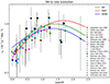 |
Fig. 1. Observed SN Ia rate as a function of redshift for different surveys, along with rate predictions for progenitor models from Greggio (2005): single degenerate, double degenerate close, double degenerate wide. |
Here, we present an assessment of the impact of uncertainties on the SN Ia rate using a simulation of the first 5 yr of LSST. As the simulation does not include other SN types, nor any correlation between the transients and the host galaxy properties, we only focus on our evaluation of the impact of uncertainties on the SN Ia rate as a function of redshift due to (i) host-galaxy association, (ii) photometric redshift, and (iii) light-curve classification, using a sample of SN Ia detected in difference images (see Sect. 3). These sources of uncertainty, affecting the choice of the SN Ia sample and their host galaxies, also affect rate measurements as a function of specific SFR or intrinsic galaxy colors from spectral energy distribution (SED) fitting. Furthermore, the sources of error studied in this work are common in all transients studies, and understanding how they propagate in a final statistical analysis would be important for most time-domain science with LSST. Measuring the SN rate and shedding light on the evolutionary channels for SNe are also goals outlined in both Dark Energy Science Collaboration2 (DESC) and Transient and Variable Stars Science Collaboration3 (TVSSC) roadmaps4 (Hambleton et al. 2023). Identifying and understanding all possible biases affecting the final measurement is therefore a crucial point before the beginning of the survey. A more thorough investigation of the SN Ia rate from LSST as a tool to discriminate between progenitor models is left to subsequent analyses.
This paper is organized as follows. Section 2 provides a short summary of the LSST strategy and design. In Sect. 3, we briefly describe the simulation and the SN sample used in our analysis. In Sect. 4, we describe the procedure of association of transients to the host galaxies, and in Sect. 5 we discuss photometric redshifts obtained from the hosts. Section 6 is dedicated to the classification of light curves and the comparison of different approaches. Finally, we present the final measurement of the SN Ia rate in Sect. 7, comparing the results with the input of the simulation and providing quantitative estimates of different sources of uncertainty. In Sect. 8, we summarize our results and discuss future perspectives.
2. LSST at the Rubin Observatory
The LSST, expected to start in 20255, will revolutionize time-domain astronomy by imaging the entire southern sky every few nights for 10 yr (Ivezić et al. 2019). The survey will be executed with the 8.4 m (6.7 m effective) Simonyi Telescope and a 3.2 gigapixel camera yielding a 9.6 deg2 field of view. The instrument is equipped with six filters, ugrizy, and is expected to have a 5σg-band magnitude depth of ∼24.5 in a single 30 s visit and ∼26.9 in the full stacked data6. The survey design will enable to cover a wide range of science goals (LSST Science Collaboration 2009), the main ones being (i) exploration of the transient and variable sky, (ii) a study of the dynamics of Solar System objects, (iii) probing dark energy and dark matter, and (iv) a map the Milky Way. Meeting most of these science goals requires scanning wide sky areas with deep images and a fast cadence. Although the exact survey strategy is not yet defined, about 90% of the observing time will be devoted to the baseline wide-fast-deep (WFD) survey mode. The remaining 10% will be used to obtain improved coverage and cadence for specific regions, called deep drilling fields (DDFs).
This exploration of the changing Universe will be boosted by the implementation of difference image analysis (DIA; Alard & Lupton 1998) on the entire dataset. DIA consists of producing deep co-added images (templates) to be subtracted from each science observation in the same region of sky. Before the subtraction, the template is resampled to the pixel coordinate system of the new image and is convolved with a kernel matching their point spread functions (PSFs). Variable sources are considered to be detected if they have a signal-to-noise ratio (S/N) greater than a threshold value (i.e., five for Rubin data products) on the resulting difference image. For each detected transient, LSST will issue an alert within 60 s of the end of the visit (defined as the end-of-image readout from the camera) to enable immediate follow-up observations with other facilities.
LSST is expected to process ∼105 transient detections per night (Ivezić et al. 2019; Graham et al. 2020a). This includes SN Ia for which we expect an increment of a factor of 100 compared to existing samples up to redshift z ∼ 1.2 (e.g., Betoule et al. 2014; Sako et al. 2018; Jones et al. 2019). Such a high number of events will dramatically reduce statistical uncertainties in the analysis of SN Ia properties and rates, which will be important both for cosmology and stellar evolution studies. The analysis of SNe is then expected to be only limited by the adopted observing strategy (affecting the sampling of light curves and the resulting classification of transients) and different sources of uncertainty, namely detection efficiency on difference images, photometric calibrations, artifact contamination levels, the reliability of the photometric redshifts of the host galaxies (e.g., precision, accuracy and fraction of catastrophic errors), and the efficiency of host-galaxy association and photometric classification algorithms. Many of these aspects have been thoroughly looked into by recent works: Sánchez et al. (2022) measured detection efficiency, magnitude limits, and photometric biases; Alves et al. (2022) and Graham et al. (2018) focused on the impact of different observing cadences on the classification of SNe and the reliability of photometric redshifts; Schmidt et al. (2020) compared different algorithms for photometric redshifts; the Photometric LSST Astronomical Time-series Classification Challenge (PLAsTiCC; The PLAsTiCC team et al. 2018; Kessler et al. 2019) and its extension ELAsTiCC7 allow different light-curve classification methods to be tested. However, all these works are oriented toward obtaining a pure sample of SN Ia for cosmology, while a study of the combination of multiple selection effects and sources of uncertainty in the specific science case of SN rate measurement (which requires a complete sample of SNe, albeit with lower purity) is still lacking. Our work complements of the previous analyses and we aim to determine the impact of host galaxy association, photometric redshift, and transient classification on the measurement of the SN Ia volumetric rate using a simulation of the first 5 yr of LSST. We discuss all of these effects one by one, in order to where improvements are needed to obtain an accurate evaluation of the SN Ia rate up to z ∼ 1 with LSST.
3. The LSST DESC DC2 Universe
To build software pipelines ready to analyze the LSST data products, DESC produced a 300 deg2 simulation of the first 5 yr of the survey as part of the Data Challenge 2 (DC2; LSST Dark Energy Science Collaboration (LSST DESC) 2021). The simulation includes LSST-like images in all six optical bands ugrizy, processed with the LSST Science Pipelines8 (v.19.0.0), and is based on the Outer Rim N-body simulation (Heitmann et al. 2019). The observing cadence is determined by the minion_10169 strategy for the WFD survey with an average cadence of ∼3 days in any filter. A smaller 1 deg2 DDF with more frequent observations (up to one per day) is also included.
Simulated sources comprise stars, galaxies, variable stars and SN Ia (but no other SN types). SN Ia light curves are simulated starting from the rest-frame spectral energy distribution (SED) of the SALT2-Extended model (Guy et al. 2010; Pierel et al. 2018), which uses five parameters: redshift (z), time at peak brightness (t0), amplitude (x0), stretch (x1), and color (c). The redshift distribution of SN Ia follows the volumetric rate rv(z) = 2.5 × 10⁻⁵(1 + z)1.5 Mpc−3 yr−1 (Dilday et al. 2008) up to z = 1.4. SNe were assigned to galaxies with an occupation probability that scales with the galaxy mass. The SN position within the host traces the light in the galaxy sampled by the surface brightness profile of the disk and the bulge. SNe at z > 1.0 are not associated to galaxies while at lower redshift, 10% of SNe were randomly injected as host-less. Correlations between the SN type and the host-galaxy properties are not included in the simulation.
The DC2 WFD region is also included in the LSST Data Preview 0 (DP010), the first of three data previews serving as an early integration test of the LSST Science Pipelines and the Rubin Science Platform (RSP). A limited number of data-rights holders have been granted access to the RSP in order to begin familiarizing themselves with the Rubin Data Products11 using a series of publicly available tutorials12. DP0 has been released in three parts:
-
DP0.1 (released on June 30, 2021) is the DESC processing of the data, focusing on static sky;
-
DP0.2 (released on June 30, 2022) is the DC2 simulation reprocessed by the Rubin staff using version 23 of the LSST Science Pipelines, and includes DIA data products;
-
DP0.3 (released on August 2, 2023) contains LSST-like catalogs of Solar System objects generated by the Solar System Science Collaboration13.
For more official references for DP0, see O’Mullane (2021), Community Engagement Team & Operations Executive Team (2022), and O’Mullane et al. (2023). All the galaxy catalogs used in this paper are extracted from DP0.2 and the codes used for the analysis have been successfully tested on the RSP, although the majority of the heavy tasks have been executed on DESC allocated space at NERSC14, which already contained all the necessary tables when this work started.
The sample of SNe Ia analyzed in this paper comes from the work by Sánchez et al. (2022), which measured magnitude limits, detection efficiency, artifact contamination levels, and biases in the selection and photometry on a subset of ∼15 deg2 of the DC2 WFD region. To perform the analysis, these authors tested the LSST DIA pipeline on the selected region, using the first year to produce their own templates and the remaining four years for detection. The smaller region of sky and the shorter survey length (5 yr instead of the planned 10) do not affect the final results.
There is a total of 5884 simulated SN Ia with z ≤ 1.0 in the processed area. This number already takes into account all the objects not detectable because of gaps between the observing seasons and objects located in sky regions with subtraction artifacts from template overlapping issues. The number of SNe with at least one detection in one filter is 2186. Nevertheless, for our analysis, we selected only sources detected on more than five distinct nights in order to sample ∼20 days on the light curve and have a more reliable classification. In cases where there were multiple visits on the same night, we took the average magnitude over all detections on that night. An example of the recovered SN Ia light curve at z = 0.16 is shown in Fig. 2. The condition on the minimum number of detections returned 600 SNe. The large drop in the number of SNe after the cut on the minimum number of detections is mainly due to the suboptimal observing cadence of the adopted survey strategy. The minion_1016 strategy adopted by DC2 is indeed relatively old, but it was most recent at the time of the simulation. Further analyses to improve the observing strategy are still ongoing, and the final cadence may improve the number of recovered SNe. Lochner et al. (2022) presented various metrics developed by DESC to analyze the cadences, highlighting the importance of low internight gaps in the redder filters for the selection of SNe. Possible improvements might also derive from a rolling cadence (Alves et al. 2023) or the higher coverage of the DDFs (Gris et al. 2023).
 |
Fig. 2. Example multiband light curve of a SN Ia with redshift z = 0.16. Different shapes and colors refer to different filters, as reported in the legend. |
The final sample of SN Ia analyzed in this work therefore consists of 600 sources (hereafter, SN Ia sample) for which we know the true host galaxy and the true simulated redshift (zspec). Throughout the paper, we treat them as a sample of candidate SN Ia, ignoring all known parameters from the simulation and using only the recovered photometric information. We first associate each SN to the host galaxy with a procedure described in Sect. 4. We then retrieve photometric redshifts for both the true (i.e., the simulation input) and the recovered host galaxies. Finally, we proceed with classification of light curves using the recovered redshifts as priors. Samples of SN Ia coming from each of these steps will produce a different distribution in redshift (see Sect. 5), thus affecting the SN Ia volumetric rate. The real case scenario consists of a sample of SNe classified as SN Ia using the photometric redshift of the associated host galaxy as a prior. Such a scenario includes a combination of all the effects analyzed in this work. We compute the SN Ia rate for different samples, alternatively analyzing each specific source of uncertainty in order to analyze the contribution of each effect separately and determine which one has the greatest impact on the final uncertainty.
4. Host-galaxy association
The association of SNe to their host galaxy is a key ingredient for the SN rate, but also for the SN photometric classification, as it provides an estimate of the SN redshift that can be used as prior in the classification (see Sect. 6). Indeed, as spectroscopic resources are limited, photometric redshifts of the host galaxies are an efficient way to obtain information on SN redshift. Moreover, knowledge of the host galaxy and its properties enables the measurement of the SN rate as a function of SFR, color, or the stellar mass of the galaxy (e.g., Sullivan et al. 2006; Botticella et al. 2017), and provides constraints on the SN progenitors (Wiseman et al. 2021).
We associate transients to galaxies using only information about the galaxy light profile and the angular separation from SNe. More complicated approaches could include any correlations between SN type and the host-galaxy properties, which are not included in this simulation. Recent reviews of host association algorithms, also using postage stamps of a field surrounding the transient, are reported in Gagliano et al. (2021) and Förster et al. (2022), the latter implementing a novel deep learning approach. We developed our own code which adapts the calculation of the directional light radius (DLR; Gupta et al. 2016) to the Rubin Data Products and produces cutouts through the RSP to evaluate the results. The DLR is the elliptical radius of a galaxy in the direction of the SN in units of arcseconds. This metric also takes the extension and the orientation of the galaxies into account, and produces more reliable physical associations than using the plain angular separation. The DLR method, using only catalog information, is fast and scalable to all kinds of extragalactic transients, as it makes no assumptions as to their nature. Our code is publicly available and ready to work with Rubin Data Products on the RSP15.
For each SN, we select host galaxy candidates in a region of 30″ radius around the SN coordinates from the catalog of static sources detected on stacked images (i.e., the LSST Object table). Such a radius is typically used in the literature and is big enough to include the hosts of extragalactic transients. The full catalog resulting from the query includes 277 852 galaxies (hereafter, candidates). Such a sample is also used in Sect. 5 to assess the quality of photometric redshifts, as it is big enough to include all typical DP0 galaxies.
We assume the isophotes of the galaxy are self-similar ellipses and get the Stokes parameters Q and U from the adaptive second moments of source intensity Ixx, Iyy, Ixy:
 (2)
(2)
 (3)
(3)
The position angle (east of north) ϕ and the axis ratio A/B of the galaxy are then
 (4)
(4)
 (5)
(5)
where k is derived from the Stokes parameters as
 (6)
(6)
We then measure the position angle α of the SN relative to the candidate host galaxy and we combine it with the angle ϕ to get the angle θ that the SN makes with the semi-major axis of the galaxy. Using the equation of an ellipse in polar coordinates with the origin at the center of the galaxy, we get the elliptical radius of a galaxy in the direction θ, which is the definition of the DLR:
 (7)
(7)
As an estimate of the semi-major axis A, we use a value of 2.5 times the Kron radius, which includes > 96% of the total flux of a galaxy (Kron 1980). Finally, we define a dimensionless quantity by normalizing the angular separation dsep between the SN and the candidate host by DLR:
 (8)
(8)
where C is the denominator of Eq. (7). In this way, we define a quantity that weights the SN radial distance by taking into account both the extension (the Kron radius, A) and the orientation (the C parameter) of the galaxy.
For each SN, we rank all candidate galaxies by increasing dDLR and pick the one with the minimum dDLR as the best host. If minimum dDLR > 4, we define the SN as host-less (SNe originally simulated as host-less in DC2 had been removed from the sample). As a further cut, we rejected candidate galaxies with i-band magnitudes magi ≥ 24.5 and with poor-quality fitting flags. These cuts reduce misassociations due to poorly estimated galaxy parameters, which is mostly the case for low-S/N sources. By looking at the distributions of candidates parameters, we also reject galaxies with Kron radii ≥7.5″ or Kron radii ≤1.4″ to reduce misassociations due to catastrophic estimates of the galaxy extension (see Fig. 3). All these cuts have an impact of only 1% on the true host galaxy sample. We point out that the DLR method is strongly dependent on the quality of galaxy fitting. The Kron radii used in this work are computed using version 23 of the LSST Science Pipelines. Newer versions may improve the quality of galaxy parameters and require different cuts.
 |
Fig. 3. Kron radii and i-band magnitudes for the entire sample of host candidate (blue dots) and true (red stars) SN host galaxies. The black square determines the region actually used for the host association, avoiding faint galaxies and catastrophic estimates of the Kron radii. |
By comparing the results of our algorithm with the simulation input, we find that 89% of SNe are correctly associated to the true host. Among the misassociations, 8 (i.e., ∼1% of the total, 12% of the erroneous cases) are recovered as host-less, and 35 (55% of the erroneous cases) are faint galaxies with magi > 22. The remaining 33% are the result of projection issues (i.e., a bright galaxy along the line of sight of a SN actually injected into a faint host), or two similar galaxies in terms of morphology and angular separation from the SN, producing a similar dDLR. Cutouts with examples of associations are reported in Fig. 4 for a correct case and two misassociations from the cases described above.
 |
Fig. 4. Cutouts around SNe (blue star) extracted with the RSP. The magenta numbers identify possible host galaxies (ranked according to the lowest dDLR), the blue x represents the best host candidate (the zeroth galaxy in the ranked list), while the red cross + is the true host galaxy of the simulation. From left to right: (i) example of a correctly associated SN, and two possible misassociation cases: (ii) very similar galaxies in terms of morphology and angular separation from the SN; (iii) example where the true host galaxy is extremely faint and not among the possible list of candidates. |
Misassociations may also alter the distribution of the parent galaxy properties, affecting the final measurement of the SN rate. Figure 5 shows how the magnitude distribution of the SN hosts changes moving from the true to the associated host galaxies (hereafter denoted with “_best”). While there is an overall agreement for bright sources, it is worth noting the excess of galaxies with magi > 22.5 for those associated with the DLR method. This will also have an effect on the accuracy of photometric redshifts, which tends to be lower with fainter sources as explained in Sect. 5.
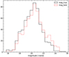 |
Fig. 5. Distribution of i-band magnitude for the SN Ia host candidates. The black solid line is the magnitude of the true host galaxy (i.e., simulation input), while the red dotted line denotes the hosts associated with the DLR method. |
The association using only the minimum angular separation has a lower efficiency of 81%. This highlights the importance of using more complex approaches, such as the DLR, to associate transients to their host galaxies. Even better results could be obtained by considering correlations between the SN type and the galaxy properties, which are not included in this simulation.
5. Photometric redshifts
We cross-matched both the catalogs of true and associated host galaxies with a catalog of photometric redshifts (zphot) for DC2 galaxies produced by Schmidt et al. (2020) with the BPZPipe code16, which employs a training set that is complete up to magi ≤ 25.0. We used the weighted mean value of the posterior probability density function (PDF) for each galaxy as a point estimate of the photometric redshift.
To assess their quality, we used the subsample of all candidates host galaxies with magi ≤ 25 and zspec ≤ 1.0, which comprises 43 161 objects. By following the approach of Graham et al. (2018), we define a zphot error as Δz = (zspec − zphot)/(1 + zphot), where zspec is the true simulated redshift. The robust standard deviation of the zphot error is evaluated in the interquartile range (IQR) containing 50% of the catalog galaxies. The value is then divided by 1.349 to convert it to the standard deviation of a Gaussian distribution (σIQR). This returns a value of σIQR = 0.05 on the catalog of all galaxies, and σIQR = 0.03 on the true host galaxies of the SN Ia. The fraction of outliers (i.e., with Δz > 3σIQR) is 7% for the catalog of all galaxy candidates and 5% for the SN Ia hosts. The comparison between the simulated and photometric redshift for both the sample of all candidate hosts and the true hosts is shown in Fig. 6, where the better agreement for the true hosts is clearly evident as they are generally more massive and brighter (see Fig. 3). The horizontal line at the bottom of the plot identifies catastrophic outliers zphot ≤ 10−5, and 15 of them refer to true SN Ia hosts. Throughout this work, we adopt a fixed value of uncertainty of 0.05 on each photometric redshift estimate, which comes from our analysis of σIQR in the galaxy catalog. This value is also consistent with our analysis of the median FWHM of the peak in the zphot PDFs.
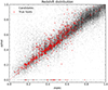 |
Fig. 6. Distribution of the true simulated redshift (zspec) and photometric redshifts (zphot) for a sample of galaxies with magi ≤ 25. Black dots are for all host candidates and red open circles are the true SN Ia hosts. |
Figure 7 shows the combined impact of photometric redshift and host galaxy association on the retrieved SN sample redshift distribution. As expected, the redshift distribution of the SN hosts appears wider when using the photometric redshift of the associate host (z_phot_best). This is especially true for faint galaxies whose uncertainty on photometric redshift is higher. We notice a peak at zphot ∼ 0 due to catastrophic outliers or SNe incorrectly associated to nearby galaxies, and a peak at zphot ∼ 0.45 mainly due to the known degeneracy between the Lyman break of galaxies at higher redshift and the Balmer break of galaxies at lower redshift (Massarotti et al. 2001; Salvato et al. 2019). These peaks, together with an excess of sources at higher redshifts, result in a decrease in the number of SNe in all the other redshift bins.
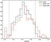 |
Fig. 7. Distribution of redshift for the SN Ia host candidates. The black one uses the true simulated redshift (zspec), the green dashed line represents the photometric redshift of the true host galaxy (zphot_true), while the red continuous distribution refers to the photometric redshift of the associated host galaxy (zphot_best). The two vertical lines define the range where we evaluate the volumetric rate and the plot is cut to z = 1.0 for visual clarity. |
In Sect. 7, we quantitatively discuss the effect of the changing distribution on the volumetric rate by considering redshift bins of 0.05 in width (which is the nominal error on photometric redshifts). The analysis is restricted to the redshift range 0.1 ≤ z ≤ 0.7 in order to avoid a catastrophic drop in the number of simulated SNe at the edges of the distribution. As shown in Fig. 7, we expect a loss of SNe in all the redshift bins with an excess at zphot ∼ 0.45. We also point out that, in principle, all the effects of bin migration arising from this work could be taken into account with a Monte Carlo analysis leading to correction coefficients (see e.g., Lasker 2020). However, estimating the proper corrections taking into account all sources of uncertainty (including those related to the detection) would require the production of more DP0-like simulations. The present work focuses on what is provided in DP0.2, as a single realisation of the Universe processed with the LSST science pipelines. The production of more complete simulations is under investigation for future works.
6. Classification
For large surveys, such as LSST, the photometric classification of transients is an essential task. Although the brokers will instantly process the nightly alert streams17, this will mainly serve as a preclassification to enable follow up of specific sources of interest with other facilities. More thorough analyses may require a posteriori classification using all the available information.
In this section, we present the results of the classification with three different approaches, which are all based on the light curves of the SN Ia sample. The first two methods involve template fitting and are part of the publicly available SuperNova ANAlysis software package (SNANA18; Kessler et al. 2009), while the last one uses a recurrent neural network (RNN) trained on light curves. For all the methods, we obtain a classification: (i) using only light curves, (ii) providing the photometric redshift of the associated host galaxy as a prior (if available19), and (iii) providing the true simulated redshift as a prior, which is the case when we have the spectroscopic redshift of the true host galaxy from other surveys.
The final results of the classification using all the methods are summarized in Table 1. Although our classification models have been trained on multiple classes, the presence of SN Ia only in the DC2 simulation prevents us from measuring the actual effect of contamination from other transients (especially from SN Ib/c). The misclassification effect will then only be a reduction in the total number of SN Ia from the original sample. We refer to upcoming works analyzing the ELAsTiCC light curves for a more through review of photometric classification.
Fraction of correctly classified SNe from the SN Ia sample using different methods.
6.1. PSNID
Photometric SuperNova IDentification (PSNID; Sako et al. 2011) is a template-fitting algorithm that calculates the reduced χ2 against a grid of SN Ia light-curve models and core-collapse SN templates in order to identify the best-matching SN type. It was first used for prioritizing spectroscopic follow-up observations for the SDSS-II SN Survey (Sako et al. 2008), and it has also been tested with SNANA simulations from the Supernova Photometric Classification Challenge (Kessler et al. 2010).
The version used here is integrated in SNANA and also computes Bayesian probabilities for different SN types. More specifically, the Bayesian evidence E for each SN type is calculated by marginalizing the product of the likelihood function and prior probabilities over the model parameter space:
 (9)
(9)
The fitting parameters are redshift z, with probability distribution P(z), extinction AV, time of maximum Tmax and distance modulus μ. In this work, priors in AV, Tmax and μ are flat, while for redshift we tested both a flat prior with P(z) = 1, and a Gaussian prior by providing the mean and sigma as described in Sect. 5 when using the photometric redshifts, and a sigma of 0.0001 when using the spectroscopic prior. For the SN Ia light curves we used the SALT2-Extended model (Pierel et al. 2018), which is the model used in the simulation, while templates for SNe core-collapse come from Vincenzi et al. (2019). SN template light curves are K-corrected using tables produced for LSST by DESC.
The Bayesian probability for each SN type is then defined as
 (10)
(10)
where
 (11)
(11)
With both Bayesian probability and χ2 available, there are many ways to select a sample of SN Ia. PSNID comes with a default criterion that takes both of them into account and defines the SN as of “unknown” type if the difference between the χ2 of two SN types is smaller than a certain threshold. However, as discussed in Kuznetsova & Connolly (2007), the minimum χ2 alone is not always a good indicator of the best SN type, and is a particularly poor indicator when small photometric errors lead to unreasonably high values of χ2. While the issue is often mitigated by artificially increasing the errors on light curves, we preferred to rely only on the Bayesian probability and selected all SNe with PIa > 0.5. With this conservative approach, we maximize the completeness of the sample, which is very important for the evaluation of the SN rate. Figure 8 shows an example of template fitting resulting in a SN Ia according to the Bayesian probability, but a SN of unknown type when using the χ2.
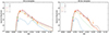 |
Fig. 8. Example of template fitting with PSNID for a SN Ia and a SN Ib/c model on the same light curve. Different colors and lines refer to different photometric bands. The left panel shows the fitting with the best Ia template, while the right panel shows the best-fitting SN Ib/c template. Although both fits seem reasonable, not allowing a straightforward classification, the type Ia has a Bayesian probability PIa = 1.0 with the redshift prior. |
The fractions of SNe correctly classified as SN Ia are very high when the redshift prior is used (95% with the associated zphot and 99% with the true simulated redshift). However, without a prior on redshift, only 44% of SNe are correctly classified, and the resulting redshift distribution is peaked towards lower values. This occurs because of a degeneracy between extinction and redshift in the light-curve reddening and highlights the importance of using priors, when available.
6.2. SALT2 fitting
Another approach often used in SN Ia cosmology consists of fitting a selected model to the light curves and taking only those candidates providing good fits (e.g., Sánchez et al. 2022; Mitra et al. 2023). The resulting sample will have high purity, which is essential for cosmological analysis, but the procedure only allows to select sources conforming to the predefined model.
As our sample contains only SN Ia, we tested this method using the software snlc_fit.exe distributed by SNANA and assuming again the SALT2-Extended model. The best fit is determined through a minimization procedure based on the CERNLIB MINUIT program20 and two iterations on each light curve. The fitting requirements are very similar to those adopted in Sánchez et al. (2022) on the same dataset:
-
stretch parameter |x1|< 3;
-
color parameter |c|< 0.3;
-
fit probability (Pfit) computed from χ2 and number of degrees of freedom satisfying Pfit > 0.05.
Similarly to what we did with PSNID, we tested the SALT2 fit both with a Gaussian prior on redshift and with no redshift prior.
The fitting procedure results in a selection efficiency of 75% when the photometric redshift of the associated galaxy is used as a prior, and 69% with no redshift information. The success fraction for the no-zphot prior scenario when using SALT2 fitting is higher than that of PSNID. The main reason for this is that PSNID is performing a more complicated classification between different classes, while here we are just fitting a single model to all our sources.
6.3. SuperNNova
Recent advantages in deep neural networks make them extremely promising for photometric classification of variable sources for large surveys such as LSST. Indeed, they can be trained on both simulated and archival data, enabling a fast multi-class analysis not limited by either costly feature extraction or template matching biases. SuperNNova21 (SNN; Möller & de Boissière 2020) is an open-source framework requiring only photometric time-series as input, with additional information (e.g., host galaxy redshift) that can be provided to improve performances. SNN includes different classification methods, such as long short-term memory (LSTM; Hochreiter & Schmidhuber 1997) recurrent neural networks (RNNs) and two Bayesian neural networks (BNNs).
As with the previous approaches, we tested SNN on our SN Ia sample both with and without redshift information using the default configuration RNN. We trained our models using a sample of synthetic light curves of all SN types with LSST-like photometric performances from ELAsTiCC. The simulation also includes spectroscopic and photometric host-galaxy redshifts for ∼5 million objects, allowing us to build a training sample with different redshift priors. We trained three different models for a binary SN Ia versus non-Ia classification: (i) light curves only, (ii) with host galaxy photometric redshift, and (iii) with spectroscopic redshift. The SNN output is a probability of being SN Ia, PIa, for each SN event. We considered as correctly classified all SN with PIa > 0.5. This resulted in 96% or 97% accuracy when the photometric or spectroscopic redshift information is used (compatible with PSNID). However, without redshift prior, only 80% of SNe are correctly classified as SN Ia.
The lower efficiencies for all the methods in the absence of redshift information show how fundamental it is to have reliable estimates of photometric redshifts and a good host association procedure. This is especially true if the number of detections and their distribution around the light-curve peak are not sufficiently sampled to enable a proper classification (see e.g., Alves et al. 2022).
7. SN Ia rate
Measurement of the SN rate requires accurate information on the survey strategy and design, both for what concerns the detection efficiency and the observing cadence. The former is usually determined with simulations and injection of point-like sources onto images, exploring a wide range of magnitudes and positions on the sky (Cappellaro et al. 2015). The impact of the latter is traditionally measured with the control time (Zwicky 1942), which is defined as the interval of time during which a SN occurring at a given redshift is expected to remain above the detection limit of the image.
However, the DC2 observing strategy is not the definitive version that will be adopted for LSST. Moreover, the main aim of this work is to analyze the impact of the sources of uncertainty that are not directly related to the survey strategy on the SN rate. For these reasons, we adopted a simplistic approach consisting in evaluating a single recovery efficiency term which takes into account both control time and detection efficiency from the simulated rate. We refer to other works for a thorough analysis of detection efficiency and magnitude limits on the DC2 simulation (Sánchez et al. 2022) and the impact of observing cadence on the classification of SNe (Alves et al. 2022).
We considered the SN Ia sample in the range 0.1 ≤ zspec ≤ 0.7 (as explained in Sect. 5), and divided it in redshift bins of 0.05 in width, which is the typical error of a photometric redshift measurement. The selected range of redshift contains 570 of the 600 SN Ia in the SN Ia sample. We define the recovery efficiency as the ratio of the number of detected sources in the SN Ia sample to the total number of simulated SN Ia in each redshift bin over an observing window of T = 3.5 yr, which is the effective observing time removing gaps between seasons. The distributions of the number of simulated and detected SN Ia in the redshift bins is shown in Fig. 9, while the ratios leading to the recovery efficiency ϵ are reported in Table 2.
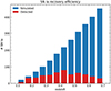 |
Fig. 9. Numbers of SN Ia simulated (blue) and detected (red, the SN Ia sample) in the redshift bins used for the measurement of the rate. |
SN Ia recovery efficiency ϵ in different redshift bins.
Depending on the adopted estimate of redshift, the distribution of SNe is different, as shown in Fig. 7. The total number of recovered SN Ia when looking at photo-z is lower than that in the simulated sample because of sources being assigned a redshift outside the selected range. Moreover, additional SN Ia are lost because of misclassifications and the absence of non-Ia contaminants. In this section, we evaluate (separately) the uncertainty contribution of photometric redshifts, host galaxy association and photometric classification on the measurement of the SN Ia rate. As a reference classification tool, we use PSNID adopting the zphot_best prior of the associated galaxy. The reasons for this choice are the flexibility of the algorithm in dealing with different SN types, the possibility to customize the output by defining an “unknown” class, and the fast execution (intrinsically parallelizable) with no requirement to build new training sets. The classification accuracy of the other multiclass algorithm (SuperNNova) is similar, and therefore the choice of the classification method does not affect the final result.
The samples used in our analysis are the following:
-
zphot_true: SN Ia sample adopting the photometric redshift of the true host galaxy instead of the true simulated redshift (this allows us to test the effect of photometric redshift).
-
zphot_best: SN Ia sample adopting the photometric redshift of the associated host galaxy (effect of photometric redshift + host galaxy association).
-
psnid_zphot_best: Sample of SNe correctly classified as SN Ia adopting the photometric redshift of the associated host galaxy as a prior (effect of photometric redshift + host galaxy association + classification uncertainties).
A first measurement of the contribution of the different effects comes from the lost fraction of SNe for the various samples Δsample, which provides an indication of the number of SN Ia lost because of incorrect photometric redshift, host association and classification. We define this value in each redshift bin as:
 (12)
(12)
where Ndetected refers to the original SN Ia sample (not affected by the uncertainties analyzed in this work) and Nrecovered is the number of SN Ia in each one of the samples defined above. The resulting values as a function of redshift are shown in Fig. 10 with different colors for the different subsets. As already noted when looking at the redshift distribution in Fig. 7, there is an overall depletion of SNe with the exception of the bins at z ∼ 0.45 and z > 0.6. The sample_psnid_zphot_best, which includes all the effects together, has an average lost fraction of 17%. However, photometric redshift alone, measured with the sample_zphot_true, has an impact of 10% and is found to be the major source of uncertainty (also affecting classification when used as prior). It is also worth noting how the different effects depend on redshift: at z > 0.4 most of the mismatch comes from the error on the photometric redshift, while lower redshifts are more affected by incorrect host-galaxy associations and incorrect photometric classification.
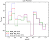 |
Fig. 10. Lost fraction of SNe in each redshift bin for the different samples, highlighting the impact of photometric redshift (zphot_true), host-galaxy association (zphot_best), and classification (psnid_zphot_best). The numbers in parentheses refer to the total number of SNe in each subset for the selected redshift range. Negative values of Δsample denote an increase in the number of sources in that redshift bin (see Eq. (12)). |
We now show how we measured the effect of the different biases on the derived SN rates. To this aim, we computed the SN Ia volumetric rate for each sample as:
 (13)
(13)
where NSN(z) is the number of SNe in each redshift bin for the selected sample, T is the observing window, (1 + z) corrects for time dilation, ϵ(z) is the SN Ia recovery efficiency defined in Table 2, and V(z) is the comoving volume for the given redshift bin:
![Mathematical equation: $$ \begin{aligned} V(z) = \frac{4\pi }{3}\frac{\Theta }{41\,253}\bigg [\frac{c}{H_0}\int ^{z2}_{z1}\frac{\mathrm{d}z^{\prime }}{\sqrt{\Omega _M(1+z^{\prime })^3+\Omega _{\Lambda }}}\bigg ]^3\,\mathrm{Mpc}^3. \end{aligned} $$](/articles/aa/full_html/2024/06/aa49012-23/aa49012-23-eq15.gif) (14)
(14)
In the previous equation, Θ is the search area of 15 deg2, z is the midpoint of the redshift interval [z1, z2], and we assumed a flat ΛCDM universe with H0 = 70 and ΩM = 0.3.
The resulting SN Ia rates for the different samples are shown in Fig. 11, along with power-law fits with the same functional form as the simulated rate from Dilday et al. (2008):
 (15)
(15)
 |
Fig. 11. SN Ia rate for the different samples, as in Fig. 10. Continuous lines are power-law fits of the rate points. Error bars due to statistical uncertainty are omitted for visual clarity. |
The fit results are summarized in Table 3. The differences between the fit parameters and the input rate (α = 2.5 and β = 1.5) show that the uncertainties not only reduce the number of SN Ia in each redshift bin, but also change the evolutionary trend of the recovered rate. The combination of the two effects hampers the use of the volumetric rate to discriminate between SN Ia progenitor models, unless the impact of these sources of uncertainty can be reduced.
Fit coefficients for all the samples.
To quantitatively address the problem, we focused on the sample_psnid_zphot_best, which represents a real case scenario combining all the uncertainties (i.e., a study of SN Ia rate with photometric data only). Figure 12 shows the recovered rate along with predictions from the progenitor models described in Sect. 1 (where the kIa factor in Eq. (1) has been fixed to  for all scenarios). It is clearly evident how LSST will reduce the scatter between the rate estimates obtained comparing multiple surveys up to z ∼ 1.0. However, biases introduced by other sources of uncertainty, such as those analyzed in this work, should still be reduced to attain optimal results. Despite Fig. 1 showing that different progenitor models have similar outcomes in the intermediate redshift range probed by LSST, the combination of LSST and higher-redshift surveys (e.g., the Nancy Grace Roman Space Telescope; Rose et al. 2021; Wang et al. 2023) could indeed allow the different scenarios to be distinguished from one another. Moreover, Greggio & Cappellaro (2019) show that the SN Ia rate as a function of host galaxy color or specific SFR leads to an even more efficient separation of the predictions of different models, once all the uncertainties have been reduced.
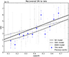 |
Fig. 12. Recovered SN Ia rate for the sample_psnid_zphot_best (the real observing case) with rate predictions of progenitor models from Greggio (2005). Error bars on the blue point are due to statistical uncertainties scaled to 10 yr over the simulated ∼15 deg2 (although we expect higher statistics with the real survey, with statistical errors reduced by more than one order of magnitude). The gray points represent rate measurement from the literature, as shown in Fig. 1. |
8. Summary and conclusions
The LSST is expected to increase the number of detected SN Ia by a factor of 100 compared to samples from previous surveys (Jones et al. 2019). This will dramatically reduce statistical uncertainties on the SN Ia rate measurement, possibly allowing us to put constraints on the SN Ia progenitors by comparing the observed rate with predictions from theoretical models. However the actual impact of all the possible sources of uncertainty on the measurement of the rate merits further analysis. While many observational biases in the selection of a good sample of SN Ia for cosmology have already been inspected in other works, here we studied the effect of uncertainties due to estimation of photometric redshift, host galaxy association and classification on the measurement of the SN Ia rate using simulated LSST images.
Data come from Sánchez et al. (2022), who executed DIA on a subset of ∼15 deg2 of the DC2 simulation. There are a total of 5884 simulated SNe with z ≤ 1.0, with 2186 of them detected in difference images. We selected only sources with more than five distinct detections in order to have a sufficiently sampled light curve for the transient classification. The analyzed SN Ia sample then consists of only 600 sources, which is an order of magnitude lower than the number of simulated SNe. The large loss of sources is mainly due to the suboptimal observing cadence of the simulated WFD region and demonstrates the need for heavily cadenced observations on smaller regions of the sky for significant statistical studies. Indeed, the definition of the best cadence is still an open issue and there are many works using simulations to provide quantitative metrics (e.g., Lochner et al. 2022).
We associate each SN Ia to its host galaxy using the DLR. Our algorithm has an association accuracy of 89% using only morphological information extracted from a single-band deep coadd image. Among the misassociations, 12% are recovered as host-less, 55% are associated to a faint galaxy with magi > 22, and the remaining 33% are a combination of projection issues or are attributable to two similar and close galaxies producing a similar dDLR. The host association could be further improved with a better estimate of the photometric parameters for faint galaxies and by also considering the correlation between SN type and host-galaxy properties (not included in the simulation).
We recovered estimates of the SN photometric redshifts from both the true and the associated host galaxy. The quality of the photometric redshift has been studied with a sample of galaxies with magi ≤ 25 and zspec ≤ 1.0. The analysis returns a robust standard deviation of σIQR = 0.05 and the fraction of outliers is 7%. The combined impact of photometric redshift and host-galaxy association results in a broadening of the SN Ia distribution in redshift. We find an excess of associated host galaxies with magi > 22.5, along with a peak at zphot ∼ 0 (due to catastrophic outliers or SNe incorrectly associated to nearby galaxies), and a peak at zphot ∼ 0.45 (mainly due to the known degeneracy between the Lyman break of galaxies at higher redshift and the Balmer break of galaxies at lower redshift).
We classified light curves with different methods, involving both template-fitting techniques (PSNID and SALT2 model fit by SNANA) and recurrent neural networks (SuperNNova). All the algorithms were executed with and without a prior on redshift, allowing us to demonstrate the improvement of classification accuracy (up to 96%) when redshift information is included. In our subsequent analysis of the SN Ia rate, we used the results of PSNID with photometric redshift of the associated host galaxy as a prior. The only effect of misclassified SNe is a decrease in the number of sources, because no other SN type is included in the simulation. A real-life scenario would also include contamination from other transients, especially from SNe of type Ib/c.
The SN Ia rate was measured on different samples in order to separately evaluate the impact of uncertainties due to photometric redshift, host-galaxy association and classification. For each sample, we divided SN Ia in redshift bins of width 0.05 (which is the typical error of a photometric redshift estimate) in the range 0.1 ≤ zspec ≤ 0.7 and normalized the rate to the input model of the DC2 simulation. The different distribution in redshift of the various samples led to an average 17% mismatch in the recovered fraction of SN Ia with respect to the original SN Ia sample. As 10% of this mismatch is due to photometric redshifts alone (which also affect the classification), we can conclude that photometric redshift estimates are a major source of limitation in the measurement of the SN Ia rate. The uncertainties not only change the number of SN Ia in each redshift bin, but also change the evolutionary trend of the recovered rate, hampering the discrimination between different progenitor models.
Despite the fact that our estimate of the uncertainties might be reduced in the near future (e.g., using better algorithms, improving the measurement procedure, including additional information, etc.), we show that they are still relevant and have a significant impact on the rate measurement; their reduction will be fundamental for precision SN Ia science, both for cosmology and stellar evolution studies. As the major source of uncertainty is due to photometric redshifts, improving their accuracy will be a priority. Graham et al. (2020b) demonstrated that adding near-infrared and near-ultraviolet photometry from the Euclid, Wide-Field InfrarRed Survey Telescope (WFIRST), and/or Cosmological Advanced Survey Telescope for Optical and ultraviolet Research (CASTOR) space telescopes can reduce both the standard deviation of photometric redshift estimates and the fraction of catastrophic outliers. The combination of Rubin and Euclid data would bring significant improvements also for other transient detection systematics, in particular for the estimate of the dust extinction bias (Guy et al. 2022). A different scenario is expected for the DDF, where improvements in the photometric redshifts could certainly be derived from the wealth of ancillary multiwavelength data, although this would mean studying a smaller area and thus a reduction in the SN statistics. Spectroscopic follow up with other facilities could also provide a good sample of galaxy properties for SN rate analysis (albeit limited to low redshift). Finally, novel deep learning techniques to measure photometric redshift have been shown to outperform other methods and might also be evaluated for LSST (e.g., Pasquet et al. 2019).
We used progenitor models from Greggio (2005) as a reference and adopted the SFH from Madau & Fragos (2017) to get predicted SN Ia rates for different progenitors. We find the combination of the uncertainties analyzed in this work to be as large as the discrepancy between the rate predictions from different progenitors. However, the scatter between the rate measurements is significantly lower than that between rate measurements obtained comparing multiple surveys, which confirms the enormous capability of LSST. It is also worth noticing that, up to z ∼ 1.0, different models have similar outcomes and it would be necessary to go to higher redshift to distinguish between them. An improvement of the redshift coverage could possibly be attained through the combination of Rubin data with Roman, which is expected to detect SN Ia up to z ∼ 3, further increasing both the dimension and the variety of the sample (Rose et al. 2021; Wang et al. 2023). Moreover, our analysis of the effect of uncertainties also has implications for the measurement the SN Ia rate as a function of host-galaxy intrinsic color or specific SFR (which has been found to offer a promising way to separate the predictions of different models as shown in Greggio & Cappellaro 2019). Unfortunately, correlations between SN type and host-galaxy properties were not included in this simulation, but their investigation will be the subject of a subsequent analysis.
http://www.lsst.org
DESC roadmap: https://lsstdesc.org/assets/pdf/docs/DESCSRMlatest.pdf
Data Products Definitions Document (DPDD; https://ls.st/dpdd).
National Energy Research Scientific Computing Center; https://www.nersc.gov/
SN Ia identified as host-less or having catastrophic photometric redshifts (i.e., zphot ≤ 10−5) are classified with a flat prior on redshift.
Acknowledgments
This paper has undergone internal review in the LSST Dark Energy Science Collaboration. We thank the internal reviewers Francisco Forster, Dominique Fouchez, and Christopher Frohmaier for their comments. We also deeply thank Richard Kessler for his help and advice throughout the work, especially on photometric classification and photometric redshifts. The DESC acknowledges ongoing support from the Institut National de Physique Nucléaire et de Physique des Particules in France; the Science & Technology Facilities Council in the United Kingdom; and the Department of Energy, the National Science Foundation, and the LSST Corporation in the United States. DESC uses resources of the IN2P3 Computing Center (CC-IN2P3–Lyon/Villeurbanne – France) funded by the Centre National de la Recherche Scientifique; the National Energy Research Scientific Computing Center, a DOE Office of Science User Facility supported by the Office of Science of the US Department of Energy under Contract No. DE-AC02-05CH11231; STFC DiRAC HPC Facilities, funded by UK BEIS National E-infrastructure capital grants; and the UK particle physics grid, supported by the GridPP Collaboration. This work was performed in part under DOE Contract DE-AC02-76SF00515. V.P. and M.T.B. were responsible for the overall analysis and interpretation of the data, and wrote the paper. E.C. contributed to the analysis and interpretation of the results. L.G. provided theoretical models for SN Ia progenitor systems. B.O.S. provided data from his previous work and hints on the analysis. A.M. contributed to photometric classification with SuperNNova, while M.S. contributed to photometric classification with PSNID. M.L.G. provided comments on photometric redshifts and helped exploiting DP0 and RSP resources. M.P. and F.B. provided final comments on the analysis and the results. All authors contributed with notes and comments to improve the clarity of the paper. A.M. is supported by the Australian Research Council Discovery Early Career Researcher Award (ARC DECRA) project number DE23010005. M.S. acknowledges support from DOE grant DE-FOA-0002424 and NSF grant AST-2108094. M.P. and V.P. acknowledge the financial contribution from PRIN-MIUR 2022 funded by the European Union – Next Generation EU, and from the Timedomes grant within the “INAF 2023 Finanziamento della Ricerca Fondamentale”. The research has made use of the following Python software packages: Astropy (Astropy Collaboration 2013, 2018), Matplotlib (Hunter 2007), Pandas (van der Walt & Millman 2010), NumPy (van der Walt et al. 2011), SciPy (Virtanen et al. 2020). Other software specific for SN analysis are cited in the paper.
References
- Alard, C., & Lupton, R. H. 1998, ApJ, 503, 325 [Google Scholar]
- Alves, C. S., Peiris, H. V., Lochner, M., et al. 2022, ApJS, 258, 23 [NASA ADS] [CrossRef] [Google Scholar]
- Alves, C. S., Peiris, H. V., Lochner, M., et al. 2023, ApJS, 265, 43 [NASA ADS] [CrossRef] [Google Scholar]
- Astropy Collaboration (Robitaille, T. P., et al.) 2013, A&A, 558, A33 [NASA ADS] [CrossRef] [EDP Sciences] [Google Scholar]
- Astropy Collaboration (Price-Whelan, A. M., et al.) 2018, AJ, 156, 123 [Google Scholar]
- Badenes, C., Hughes, J. P., Bravo, E., & Langer, N. 2007, ApJ, 662, 472 [NASA ADS] [CrossRef] [Google Scholar]
- Barbary, K., Aldering, G., Amanullah, R., et al. 2012, ApJ, 745, 31 [NASA ADS] [CrossRef] [Google Scholar]
- Betoule, M., Kessler, R., Guy, J., et al. 2014, A&A, 568, A22 [NASA ADS] [CrossRef] [EDP Sciences] [Google Scholar]
- Blanc, G., Afonso, C., Alard, C., et al. 2004, A&A, 423, 881 [NASA ADS] [CrossRef] [EDP Sciences] [Google Scholar]
- Botticella, M. T., Riello, M., Cappellaro, E., et al. 2008, A&A, 479, 49 [NASA ADS] [CrossRef] [EDP Sciences] [Google Scholar]
- Botticella, M. T., Cappellaro, E., Greggio, L., et al. 2017, A&A, 598, A50 [NASA ADS] [CrossRef] [EDP Sciences] [Google Scholar]
- Cappellaro, E., Evans, R., & Turatto, M. 1999, A&A, 351, 459 [NASA ADS] [Google Scholar]
- Cappellaro, E., Botticella, M. T., Pignata, G., et al. 2015, A&A, 584, A62 [NASA ADS] [CrossRef] [EDP Sciences] [Google Scholar]
- Cappellaro, E., Botticella, M. T., Pignata, G., et al. 2016, VizieR Online Data Catalog: J/A+A/584/A62 [Google Scholar]
- Community Engagement Team& Operations Executive Team 2022, Guidelines for Community Participation in Data Preview 0, Vera C. Rubin Observatory Technical Note [Google Scholar]
- Dahlen, T., Strolger, L.-G., & Riess, A. G. 2008, ApJ, 681, 462 [NASA ADS] [CrossRef] [Google Scholar]
- Dhawan, S., Leibundgut, B., Spyromilio, J., & Blondin, S. 2016, A&A, 588, A84 [NASA ADS] [CrossRef] [EDP Sciences] [Google Scholar]
- Dilday, B., Kessler, R., Frieman, J. A., et al. 2008, ApJ, 682, 262 [Google Scholar]
- Dilday, B., Smith, M., Bassett, B., et al. 2010, ApJ, 713, 1026 [NASA ADS] [CrossRef] [Google Scholar]
- Foley, R. J., Simon, J. D., Burns, C. R., et al. 2012, ApJ, 752, 101 [CrossRef] [Google Scholar]
- Förster, F., Muñoz Arancibia, A. M., Reyes-Jainaga, I., et al. 2022, AJ, 164, 195 [CrossRef] [Google Scholar]
- Frohmaier, C., Sullivan, M., Nugent, P. E., et al. 2019, MNRAS, 486, 2308 [CrossRef] [Google Scholar]
- Gagliano, A., Narayan, G., Engel, A., Carrasco Kind, M., & LSST Dark Energy Science Collaboration 2021, ApJ, 908, 170 [NASA ADS] [CrossRef] [Google Scholar]
- Graham, M. L., Connolly, A. J., Ivezić, Ž., et al. 2018, AJ, 155, 1 [Google Scholar]
- Graham, M. L., Bellm, E., Guy, L., et al. 2020a, LSST Alerts: Key Numbers, Vera C. Rubin Observatory Data Management Technical Note [Google Scholar]
- Graham, M. L., Connolly, A. J., Wang, W., et al. 2020b, AJ, 159, 258 [Google Scholar]
- Graur, O., & Maoz, D. 2013, MNRAS, 430, 1746 [NASA ADS] [CrossRef] [Google Scholar]
- Graur, O., & Woods, T. E. 2019, MNRAS, 484, L79 [NASA ADS] [CrossRef] [Google Scholar]
- Graur, O., Poznanski, D., Maoz, D., et al. 2011, MNRAS, 417, 916 [Google Scholar]
- Graur, O., Rodney, S. A., Maoz, D., et al. 2014, ApJ, 783, 28 [NASA ADS] [CrossRef] [Google Scholar]
- Greggio, L. 2005, A&A, 441, 1055 [NASA ADS] [CrossRef] [EDP Sciences] [Google Scholar]
- Greggio, L. 2010, MNRAS, 406, 22 [CrossRef] [Google Scholar]
- Greggio, L., & Cappellaro, E. 2019, A&A, 625, A113 [NASA ADS] [CrossRef] [EDP Sciences] [Google Scholar]
- Gris, P., Regnault, N., Awan, H., et al. 2023, ApJS, 264, 22 [NASA ADS] [CrossRef] [Google Scholar]
- Gupta, R. R., Kuhlmann, S., Kovacs, E., et al. 2016, AJ, 152, 154 [NASA ADS] [CrossRef] [Google Scholar]
- Guy, J., Sullivan, M., Conley, A., et al. 2010, A&A, 523, A7 [NASA ADS] [CrossRef] [EDP Sciences] [Google Scholar]
- Guy, L. P., Cuillandre, J. C., Bachelet, E., et al. 2022, https://doi.org/10.5281/zenodo.5836022 [Google Scholar]
- Hambleton, K. M., Bianco, F. B., Street, R., et al. 2023, PASP, 135, 105002 [NASA ADS] [CrossRef] [Google Scholar]
- Hardin, D., Afonso, C., Alard, C., et al. 2000, A&A, 362, 419 [NASA ADS] [Google Scholar]
- Heitmann, K., Finkel, H., Pope, A., et al. 2019, ApJS, 245, 16 [NASA ADS] [CrossRef] [Google Scholar]
- Hochreiter, S., & Schmidhuber, J. 1997, Neural Comput., 9, 1735 [CrossRef] [Google Scholar]
- Horesh, A., Poznanski, D., Ofek, E. O., & Maoz, D. 2008, MNRAS, 389, 1871 [NASA ADS] [CrossRef] [Google Scholar]
- Hunter, J. D. 2007, Comput. Sci. Eng., 9, 90 [NASA ADS] [CrossRef] [Google Scholar]
- Iben, I., Jr., & Tutukov, A. V. 1984, ApJS, 54, 335 [NASA ADS] [CrossRef] [Google Scholar]
- Ivezić, Ž., Kahn, S. M., Tyson, J. A., et al. 2019, ApJ, 873, 111 [Google Scholar]
- Jones, D. O., Scolnic, D. M., Foley, R. J., et al. 2019, ApJ, 881, 19 [Google Scholar]
- Kelly, P. L., Fox, O. D., Filippenko, A. V., et al. 2014, ApJ, 790, 3 [NASA ADS] [CrossRef] [Google Scholar]
- Kerzendorf, W. E., Do, T., de Mink, S. E., et al. 2019, A&A, 623, A34 [NASA ADS] [CrossRef] [EDP Sciences] [Google Scholar]
- Kessler, R., Bernstein, J. P., Cinabro, D., et al. 2009, PASP, 121, 1028 [Google Scholar]
- Kessler, R., Conley, A., Jha, S., & Kuhlmann, S. 2010, ArXiv e-prints [arXiv:1001.5210] [Google Scholar]
- Kessler, R., Narayan, G., Avelino, A., et al. 2019, PASP, 131, 094501 [NASA ADS] [CrossRef] [Google Scholar]
- Kron, R. G. 1980, ApJS, 43, 305 [Google Scholar]
- Kuznetsova, N. V., & Connolly, B. M. 2007, ApJ, 659, 530 [NASA ADS] [CrossRef] [Google Scholar]
- Lasker, J. E. 2020, Ph.D. Thesis, University of Chicago [Google Scholar]
- Li, W., Leaman, J., Chornock, R., et al. 2011, MNRAS, 412, 1441 [NASA ADS] [CrossRef] [Google Scholar]
- Livio, M., & Mazzali, P. 2018, Phys. Rep., 736, 1 [Google Scholar]
- Lochner, M., Scolnic, D., Almoubayyed, H., et al. 2022, ApJS, 259, 58 [NASA ADS] [CrossRef] [Google Scholar]
- LSST Dark Energy Science Collaboration (LSST DESC) (Abolfathi, B., et al.) 2021, ApJS, 253, 31 [CrossRef] [Google Scholar]
- LSST Science Collaboration (Abell, P. A., et al.) 2009, ArXiv e-prints [arXiv:0912.0201] [Google Scholar]
- Madau, P., & Fragos, T. 2017, ApJ, 840, 39 [Google Scholar]
- Maoz, D., Mannucci, F., & Brandt, T. D. 2012, MNRAS, 426, 3282 [NASA ADS] [CrossRef] [Google Scholar]
- Massarotti, M., Iovino, A., Buzzoni, A., & Valls-Gabaud, D. 2001, A&A, 380, 425 [NASA ADS] [CrossRef] [EDP Sciences] [Google Scholar]
- Melinder, J., Dahlen, T., Mencía Trinchant, L., et al. 2012, A&A, 545, A96 [NASA ADS] [CrossRef] [EDP Sciences] [Google Scholar]
- Mitra, A., Kessler, R., More, S., Hlozek, R., & LSST Dark Energy Science Collaboration 2023, ApJ, 944, 212 [NASA ADS] [CrossRef] [Google Scholar]
- Möller, A., & de Boissière, T. 2020, MNRAS, 491, 4277 [CrossRef] [Google Scholar]
- Okumura, J. E., Ihara, Y., Doi, M., et al. 2014, PASJ, 66, 49 [NASA ADS] [Google Scholar]
- O’Mullane, W. 2021, Data Preview 0: Definition and Planning, Vera C. Rubin Observatory Technical Note [Google Scholar]
- O’Mullane, W., Alsayyad, Y., Chiang, H. F., et al. 2023, Data Preview 0.2 and Operations Rehearsal for DRP, Vera C. Rubin Observatory Technical Note [Google Scholar]
- Pain, R., Fabbro, S., Sullivan, M., et al. 2002, ApJ, 577, 120 [NASA ADS] [CrossRef] [Google Scholar]
- Pasquet, J., Bertin, E., Treyer, M., Arnouts, S., & Fouchez, D. 2019, A&A, 621, A26 [NASA ADS] [CrossRef] [EDP Sciences] [Google Scholar]
- Perlmutter, S., Aldering, G., Goldhaber, G., et al. 1999, ApJ, 517, 565 [Google Scholar]
- Perrett, K., Sullivan, M., Conley, A., et al. 2012, AJ, 144, 59 [NASA ADS] [CrossRef] [Google Scholar]
- Phillips, M. M. 1993, ApJ, 413, L105 [Google Scholar]
- Pierel, J. D. R., Rodney, S., Avelino, A., et al. 2018, PASP, 130, 114504 [NASA ADS] [CrossRef] [Google Scholar]
- Riess, A. G., Filippenko, A. V., Challis, P., et al. 1998, AJ, 116, 1009 [Google Scholar]
- Rodney, S. A., & Tonry, J. L. 2010, ApJ, 723, 47 [NASA ADS] [CrossRef] [Google Scholar]
- Rodney, S. A., Riess, A. G., Strolger, L.-G., et al. 2014, AJ, 148, 13 [Google Scholar]
- Rose, B. M., Aldering, G., Dai, M., et al. 2021, ArXiv e-prints [arXiv:2104.01199] [Google Scholar]
- Sako, M., Bassett, B., Becker, A., et al. 2008, AJ, 135, 348 [Google Scholar]
- Sako, M., Bassett, B., Connolly, B., et al. 2011, ApJ, 738, 162 [NASA ADS] [CrossRef] [Google Scholar]
- Sako, M., Bassett, B., Becker, A. C., et al. 2018, PASP, 130, 064002 [NASA ADS] [CrossRef] [Google Scholar]
- Salvato, M., Ilbert, O., & Hoyle, B. 2019, Nat. Astron., 3, 212 [NASA ADS] [CrossRef] [Google Scholar]
- Sánchez, B. O., Kessler, R., Scolnic, D., et al. 2022, ApJ, 934, 96 [CrossRef] [Google Scholar]
- Schaefer, B. E., & Pagnotta, A. 2012, Nature, 481, 164 [NASA ADS] [CrossRef] [Google Scholar]
- Schmidt, S. J., Malz, A. I., Soo, J. Y. H., et al. 2020, MNRAS, 499, 1587 [Google Scholar]
- Strolger, L.-G., Rodney, S. A., Pacifici, C., Narayan, G., & Graur, O. 2020, ApJ, 890, 140 [NASA ADS] [CrossRef] [Google Scholar]
- Sullivan, M., Le Borgne, D., Pritchet, C. J., et al. 2006, ApJ, 648, 868 [NASA ADS] [CrossRef] [Google Scholar]
- The PLAsTiCC team, Allam, T., Jr., Bahmanyar, A., et al. 2018, ArXiv e-prints [arXiv:1810.00001] [Google Scholar]
- Tonry, J. L., Schmidt, B. P., Barris, B., et al. 2003, ApJ, 594, 1 [NASA ADS] [CrossRef] [Google Scholar]
- Tripp, R., & Branch, D. 1999, ApJ, 525, 209 [NASA ADS] [CrossRef] [Google Scholar]
- van der Walt, S., & Millman, J., eds. 2010, in Proceedings of the 9th Python in Science Conference [Google Scholar]
- van der Walt, S., Colbert, S. C., & Varoquaux, G. 2011, Comput. Sci. Eng., 13, 22 [Google Scholar]
- Vincenzi, M., Sullivan, M., Firth, R. E., et al. 2019, MNRAS, 489, 5802 [NASA ADS] [CrossRef] [Google Scholar]
- Virtanen, P., Gommers, R., Oliphant, T. E., et al. 2020, Nat. Methods, 17, 261 [Google Scholar]
- Wang, B., & Han, Z. 2012, New Astron. Rev., 56, 122 [CrossRef] [Google Scholar]
- Wang, K. X., Scolnic, D., Troxel, M. A., et al. 2023, MNRAS, 523, 3874 [NASA ADS] [CrossRef] [Google Scholar]
- Webbink, R. F. 1984, ApJ, 277, 355 [NASA ADS] [CrossRef] [Google Scholar]
- Whelan, J., & Iben, I., Jr. 1973, ApJ, 186, 1007 [Google Scholar]
- Wiseman, P., Sullivan, M., Smith, M., et al. 2021, MNRAS, 506, 3330 [NASA ADS] [Google Scholar]
- Zwicky, F. 1942, ApJ, 96, 28 [NASA ADS] [CrossRef] [Google Scholar]
All Tables
Fraction of correctly classified SNe from the SN Ia sample using different methods.
All Figures
|
Fig. 1. Observed SN Ia rate as a function of redshift for different surveys, along with rate predictions for progenitor models from Greggio (2005): single degenerate, double degenerate close, double degenerate wide. |
| In the text | |
|
Fig. 2. Example multiband light curve of a SN Ia with redshift z = 0.16. Different shapes and colors refer to different filters, as reported in the legend. |
| In the text | |
|
Fig. 3. Kron radii and i-band magnitudes for the entire sample of host candidate (blue dots) and true (red stars) SN host galaxies. The black square determines the region actually used for the host association, avoiding faint galaxies and catastrophic estimates of the Kron radii. |
| In the text | |
|
Fig. 4. Cutouts around SNe (blue star) extracted with the RSP. The magenta numbers identify possible host galaxies (ranked according to the lowest dDLR), the blue x represents the best host candidate (the zeroth galaxy in the ranked list), while the red cross + is the true host galaxy of the simulation. From left to right: (i) example of a correctly associated SN, and two possible misassociation cases: (ii) very similar galaxies in terms of morphology and angular separation from the SN; (iii) example where the true host galaxy is extremely faint and not among the possible list of candidates. |
| In the text | |
|
Fig. 5. Distribution of i-band magnitude for the SN Ia host candidates. The black solid line is the magnitude of the true host galaxy (i.e., simulation input), while the red dotted line denotes the hosts associated with the DLR method. |
| In the text | |
|
Fig. 6. Distribution of the true simulated redshift (zspec) and photometric redshifts (zphot) for a sample of galaxies with magi ≤ 25. Black dots are for all host candidates and red open circles are the true SN Ia hosts. |
| In the text | |
|
Fig. 7. Distribution of redshift for the SN Ia host candidates. The black one uses the true simulated redshift (zspec), the green dashed line represents the photometric redshift of the true host galaxy (zphot_true), while the red continuous distribution refers to the photometric redshift of the associated host galaxy (zphot_best). The two vertical lines define the range where we evaluate the volumetric rate and the plot is cut to z = 1.0 for visual clarity. |
| In the text | |
|
Fig. 8. Example of template fitting with PSNID for a SN Ia and a SN Ib/c model on the same light curve. Different colors and lines refer to different photometric bands. The left panel shows the fitting with the best Ia template, while the right panel shows the best-fitting SN Ib/c template. Although both fits seem reasonable, not allowing a straightforward classification, the type Ia has a Bayesian probability PIa = 1.0 with the redshift prior. |
| In the text | |
|
Fig. 9. Numbers of SN Ia simulated (blue) and detected (red, the SN Ia sample) in the redshift bins used for the measurement of the rate. |
| In the text | |
|
Fig. 10. Lost fraction of SNe in each redshift bin for the different samples, highlighting the impact of photometric redshift (zphot_true), host-galaxy association (zphot_best), and classification (psnid_zphot_best). The numbers in parentheses refer to the total number of SNe in each subset for the selected redshift range. Negative values of Δsample denote an increase in the number of sources in that redshift bin (see Eq. (12)). |
| In the text | |
|
Fig. 11. SN Ia rate for the different samples, as in Fig. 10. Continuous lines are power-law fits of the rate points. Error bars due to statistical uncertainty are omitted for visual clarity. |
| In the text | |
|
Fig. 12. Recovered SN Ia rate for the sample_psnid_zphot_best (the real observing case) with rate predictions of progenitor models from Greggio (2005). Error bars on the blue point are due to statistical uncertainties scaled to 10 yr over the simulated ∼15 deg2 (although we expect higher statistics with the real survey, with statistical errors reduced by more than one order of magnitude). The gray points represent rate measurement from the literature, as shown in Fig. 1. |
| In the text | |
Current usage metrics show cumulative count of Article Views (full-text article views including HTML views, PDF and ePub downloads, according to the available data) and Abstracts Views on Vision4Press platform.
Data correspond to usage on the plateform after 2015. The current usage metrics is available 48-96 hours after online publication and is updated daily on week days.
Initial download of the metrics may take a while.