| Issue |
A&A
Volume 694, February 2025
|
|
|---|---|---|
| Article Number | A166 | |
| Number of page(s) | 14 | |
| Section | Interstellar and circumstellar matter | |
| DOI | https://doi.org/10.1051/0004-6361/202452598 | |
| Published online | 11 February 2025 | |
The ALMA-ATOMS survey: Vibrationally excited HC3N lines in hot cores
1
School of Physics and Astronomy, Yunnan University,
Kunming
650091,
PR
China
2
Shanghai Astronomical Observatory, Chinese Academy of Sciences,
80 Nandan Road,
Shanghai
200030,
PR
China
3
Jet Propulsion Laboratory, California Institute of Technology,
4800 Oak Grove Drive,
Pasadena
CA
91109,
USA
4
Department of Physics, Faculty of Science, Kunming University of Science and Technology,
Kunming
650500,
PR
China
5
Xinjiang Astronomical Observatory, Chinese Academy of Sciences,
150 Science 1-Stree, Urumqi,
Xinjiang
830011,
PR
China
6
Xinjiang Key Laboratory of Radio Astrophysics,
150 Science 1-Street, Urumqi,
Xinjiang
830011,
PR
China
7
Departamento de Astronomía, Universidad de Chile, Las Condes,
7591245
Santiago,
Chile
8
Chinese Academy of Sciences South America Center for Astronomy, National Astronomical Observatories, CAS,
Beijing
100101,
PR
China
9
University of Chinese Academy of Sciences,
Beijing
100049,
PR
China
10
Institute of Astrophysics, School of Physics and Electronical Science, Chuxiong Normal University,
Chuxiong
675000,
PR
China
11
Department of Earth and Planetary Sciences, Institute of Science Tokyo, Meguro,
Tokyo
152-8551,
Japan
12
National Astronomical Observatory of Japan, National Institutes of Natural Sciences,
2-21-1 Osawa, Mitaka,
Tokyo
181-8588,
Japan
13
Department of Astronomical Science, SOKENDAI (The Graduate University for Advanced Studies),
2-21-1 Osawa, Mitaka,
Tokyo
181-8588,
Japan
14
Rosseland Centre for Solar Physics, University of Oslo,
PO Box 1029 Blindern,
0315
Oslo,
Norway
15
Institute of Theoretical Astrophysics, University of Oslo,
PO Box 1029 Blindern,
0315
Oslo,
Norway
16
Physical Research Laboratory, Navrangpura,
Ahmedabad
380 009,
India
17
Instituto de Astronomïa, Universidad Católica del Norte,
Antofagasta,
Chile
18
Max Planck Institute for Astronomy,
Königstuhl 17,
69117
Heidelberg,
Germany
19
Korea Astronomy and Space Science Institute,
776 Daedeokdaero, Yuseong-gu,
Daejeon
34055,
Republic of Korea
20
University of Science and Technology, Korea (UST),
217 Gajeong-ro, Yuseong-gu,
Daejeon
34113,
Republic of Korea
21
Department of Astronomy, Eötvös Loránd University,
Pázmány Péter sétány 1/A,
1117,
Budapest,
Hungary
22
University of Debrecen, Faculty of Science and Technology,
Egyetemtér 1,
4032
Debrecen,
Hungary
23
Department of Mathematical Sciences, University of South Africa,
Cnr Christian de Wet Rd and Pioneer Avenue, Florida Park,
1709
Roodepoort,
South Africa
24
Centre for Space Research, North-West University, Potchefstroom Campus,
Private Bag X6001,
Potchefstroom
2520,
South Africa
25
Department of Physics and Astronomy, Faculty of Physical Sciences, University of Nigeria,
Carver Building, 1 University Road,
Nsukka
410001,
Nigeria
26
I. Physikalisches Institut, Universität zu Köln,
Zülpicher Straße 77,
50937
Köln,
Germany
27
Kavli Institute for Astronomy and Astrophysics, Peking University,
5 Yiheyuan Road, Haidian District,
Beijing
100871,
China
28
School of Physics and Astronomy, Sun Yat-sen University,
2 Daxue Road, Zhuhai,
Guangdong
519082,
PR
China
★ Corresponding authors; This email address is being protected from spambots. You need JavaScript enabled to view it.
; This email address is being protected from spambots. You need JavaScript enabled to view it.
; This email address is being protected from spambots. You need JavaScript enabled to view it.
Received:
14
October
2024
Accepted:
16
December
2024
Abstract
Context. Interstellar molecules are excellent tools for studying the physical and chemical environments of massive star-forming regions. In particular, the vibrationally excited HC3N (HC3N*) lines are the key tracers for probing hot cores environments.
Aims. We present the Atacama Large Millimeter/submillimeter Array (ALMA) 3 mm observations of HC3N* lines in 60 hot cores and investigate how the physical conditions affect the excitation of HC3N* transitions.
Methods. We used the XCLASS for line identification. Under the assumption of local thermodynamic equilibrium, we derived the rotation temperature and column density of HC3N* transitions in hot cores. Additionally, we calculated the H2 column density and number density, along with the abundance of HC3N* relative to H2, to enable a comparison of the physical properties of hot cores with different numbers of HC3N* states.
Results. We have detected HC3N* lines in 52 hot cores, 29 of which show more than one vibrationally excited state. Hot cores with higher gas temperatures have more detections of these vibrationally excited lines. The excitation of HC3N* requires dense environments, and its spatial distribution is affected by the presence of UC HII regions. The observed column density of HC3N* contributes to the number of HC3N* states in hot-core environments.
Conclusions. After analyzing the various factors influencing HC3N* excitation in hot cores, we conclude that the excitation of HC3N* is mainly driven by mid-IR pumping, while collisional excitation is ineffective.
Key words: stars: formation / ISM: abundances / HII regions / ISM: molecules
© The Authors 2025
 Open Access article, published by EDP Sciences, under the terms of the Creative Commons Attribution License (https://creativecommons.org/licenses/by/4.0), which permits unrestricted use, distribution, and reproduction in any medium, provided the original work is properly cited.
This article is published in open access under the Subscribe to Open model. This email address is being protected from spambots. You need JavaScript enabled to view it. to support open access publication.
1 Introduction
Massive star-forming regions represent some of the most dynamic and intriguing environments in the cosmos. These areas serve as cosmic crucibles where gravitational forces, radiation, and turbulent motion interact to shape the birth and evolution of stellar progenitors (Zhang & Li 2017; Tang et al. 2018; Motte et al. 2018; Lu et al. 2020; Yue et al. 2021; Saha et al. 2022; Rosen 2022; Luo et al. 2024). Motivated by the fundamental importance of massive star-forming regions, researchers have long sought to dissect the molecular landscapes that characterize these environments (for comprehensive reviews, see Herbst & van Dishoeck 2009; Gerin et al. 2016; van Dishoeck 2018; Jørgensen et al. 2020). Among the myriad molecular species, cyanoacetylene (HC3N) stands out as a particularly intriguing tracer of dense and warm gas surrounding newly forming stars (Chung et al. 1991; Bergin et al. 1996; Yu et al. 2019) and energetic processes in highly obscured regions (Rico-Villas et al. 2021). Previous observations have laid important groundwork in the investigation of HC3N lines in massive star-forming regions (Li et al. 2017; Taniguchi et al. 2018; He et al. 2021), shedding light on their abundance patterns, spatial distributions, and excitation mechanisms.
The shortest cyanopolyyne, HC3N (H–C≡C–C≡N), possesses one CN triple bond and one CC triple bond. As a linear molecule, HC3N is widespread in the interstellar medium (ISM) and has been detected in various astronomical sources both in the Milky Way (Turner 1971; Kunde et al. 1981; Li & Goldsmith 2012; Velilla Prieto et al. 2015; Zinchenko et al. 2021; Liu et al. 2024) and in external galaxies (Mauersberger et al. 1990; Wang et al. 2020; Martín et al. 2021). The excitation of HC3N can be driven by the absorption of mid-IR photons and/or collisions with H2 (Rico-Villas et al. 2020). Because the linear structure of HC3N lacks a center of symmetry, the spectra produced by its transitions are complex. Experiments by Yamada & Creswell (1986) and Thorwirth et al. (2000) have given information on the transitions of rotational spectra of various vibrationally excited HC3N states in the millimeter and submillimeter wave bands. HC3N exhibits seven normal vibrations: four stretching vibrations (v1–v4) of Σ symmetry, and three doubly degenerate bending vibrations (v5–v7) of Π symmetry (Mallinson & Fayt 1976). The characteristics of these seven vibrational states are summarized in Table 1 (Ranković et al. 2018). The vibrationally excited state of HC3N refers to a specific state with higher vibrational energy, resulting from the excitation of a vibrational mode after the molecule absorbs energy. Experiments show that higher vibrational energy levels require a higher impact energy to be collisionally excited (Leach et al. 2014). In astrophysical environments, the critical densities (ncrit) for collisional excitation of the v7 = 1, v6 = 1, v5 = 1, and v4 = 1 levels at 300 K are 4 × 10⁸, 3 × 10¹¹, 7 × 10¹², and 2 × 1010 cm−3, respectively (Wyrowski et al. 1999). Therefore, in this work, only the low-lying vibrational modes (v4, v5, v6, and v7) with one or multiple vibrationally excited states are investigated, as detected in the ALMA band 3 survey.
Despite significant progress, gaps persist in our understanding, particularly in relation to the precise role of vibrationally excited HC3N (abbreviated as HC3N*) in probing the conditions prevailing within hot cores. Clarifying these issues is essential for constructing comprehensive models of massive star formation and refining our understanding of the underlying physics. Spurred by the potential to unveil crucial details about the physical conditions operating in extreme environments, attention has turned to the study of HC3N* lines within hot cores (Goldsmith et al. 1982; Wyrowski et al. 1999; de Vicente et al. 2000; Costagliola & Aalto 2010; Belloche et al. 2013; Peng et al. 2017; Pagani et al. 2017; Taniguchi et al. 2022). The spectral information of the vibrationally excited states can reveal the behavior of HC3N molecules in different energy states and their distribution in the ISM. Particularly in high-temperature environments, the study of vibrationally excited states is significant for understanding molecular excitation and chemical reaction processes (Esplugues et al. 2013).
Against this backdrop, the primary objective of this paper is to present a detailed examination of HC3N* lines in massive star-forming regions and provide a comprehensive understanding of the role HC3N* plays in studying the inner physical conditions of hot cores. By systematically exploring the characteristics of different HC3N* states, this study intends to elucidate their observational properties and the physical processes shaping their spectral lines. The structure of this paper is organized as follows: In Sect. 2 we describe the ALMA observations and the data reduction process. Section 3 presents the fundamental results on the detection of HC3N* lines and the preliminary analysis of the derived physical parameters. In Sect. 4, we discuss the results of the study in depth, identifying the physical properties and the vibrational excitation conditions of HC3N. Finally, Sect. 5 outlines the key conclusions of this paper.
Lowest vibrational modes of HC3N.
2 Observations and data reduction
2.1 ALMA observations
The ATOMS, standing for ALMA Three-millimeter Observations of Massive Star-forming regions, is an ALMA band 3 survey aimed at studying the physical and chemical conditions of 146 massive star-forming regions (Liu et al. 2020; Project ID: 2019.1.00685.S; PI: Tie Liu). The observations were conducted from September to mid-November 2019 and included both the Atacama Compact 7 m Array (ACA) and the 12 m array (C43-2 or C43-3 configuration). SPWs 7 and 8 are tuned in the upper sideband of the observations, which have a bandwidth of 1875 MHz and a spectral resolution of approximately 1.6 km s−1. SPWs 7 and 8 were primarily used for continuum imaging and line surveys, with center frequencies of ~98 505 MHz and 100 454 MHz, respectively. In the ATOMS project, due to the high resolution and minimal flux loss in the dense molecular line tracers, we exclusively rely on 12 m array data to identify molecular lines and hot cores.
2.2 Data calibration and imaging
Data reduction and image processing were conducted using version 5.6 of the Common Astronomy Software Applications (CASA; McMullin et al. 2007; CASA Team 2022). The ACA data and 12 m array data were calibrated separately, and the 12 m array data were chosen for identifying cloud cores and molecular lines. For the continuum maps, line-free channels were selected in SPW 7 and SPW 8, with a central frequency of approximately 99 404 MHz. Line cubes were produced for each SPW with their native spectral resolution, and the maximum recoverable angular scales were approximately 60 arcsec. All images were corrected for primary beam. The 12 m data for the 146 clumps have an angular resolution of approximately 1.2–1.9 arcsec (the linear scale angular resolution are listed in Col. 4 of Tables C.1 to C.4), with a mean sensitivity of approximately 0.4 mJy beam−1 for the continuum and better than 10 mJy beam−1 per channel for the lines. By using three complex organic molecules (COMs), namely C2H5CN, CH3OCHO, and CH3OH, as probes for hot cores, Qin et al. (2022) successfully identified 60 hot cores, which were selected as the sample for our study.
3 Methods and results
3.1 HC3N* line identification
We conducted a search for all vibrationally excited lines of HC3N in 60 hot cores. The molecular lines were obtained from the peak position of each hot core. Precise line identification was performed using the eXtended CASA Line Analysis Software Suite (XCLASS; Möller et al. 2017)1, assuming local thermodynamic equilibrium (LTE). The Cologne Database for Molecular Spectroscopy (CDMS; Müller et al. 2001, 2005; Endres et al. 2016)2 and the Jet Propulsion Laboratory (JPL) molecular databases (Pickett et al. 1998)3, accessed through XCLASS, provided line parameters such as rest frequency, quantum number (QN), dipole-weighted transition dipole matrix elements (Sijμ2), Einstein A coefficient (Aij), and upper energy (Eu). In this survey, we detected a total of seven types of HC3N* lines in 52 hot cores: v7 = 1, v7 = 2, v7 = 3, v6 = 1, v6 = v7 = 1, v5 = 1, and v4 = 1. The seven HC3N states include 18 transitions in SPW 8 and none in SPW 7, all corresponding to the same J=11 − 10 transition. The relevant parameters are listed in Table A.1. One HC3N v=0 (J=11 − 10) line was also detected in SPW 8 at the rest frequency ~100 076 MHz, which indicates that all 52 hot cores contain HC3N molecules. The determination of each line was based on its velocity offset, which was almost the same as the systemic source velocity (see Liu et al. (2020) for specific values), and with a line intensity above the 3σ detection level.
The distribution of HC3N* lines is concentrated in SPW 8, with a broad range of upper energy levels ranging from 349 to 1274 K. We used XCLASS to fit the physical parameters, including rotation temperature, column density, line width, and velocity offset, by setting the deconvolved size of the continuum core, rotation temperature, source-averaged column density, line width, and velocity offset as free parameters in the fitting process, with a setup of an isotope ratio of 1 (i.e., the same abundance) for HC3N* in each vibrationally excited state. The physical parameters for each vibrationally excited state were determined simultaneously only when there were three or more corresponding lines. However, for hot cores with only v7 = 1 lines, it was not possible to derive the physical parameters as only two emission lines were detected. Ultimately, we were able to fit 29 hot cores with more than three vibrationally excited lines. The catalog of detected HC3N* lines toward hot cores, along with the corresponding rotation temperatures and column densities, is presented in Table B.1. Eight of the 60 hot cores in our sample show no HC3N* emission. This accounts for 13% of the total detections. Additionally, 23 hot cores exclusively display v7 = 1 emission, which represents 38% of the total hot core detections. The detection rates for v7 = 1, v7 = 2, v6 = 1, v5 = 1, v7 = 3, v6 = v7 = 1, and v4 = 1 are 87%, 48%, 45%, 27%, 27%, 25%, and 3%, respectively. In Fig. 1, we present sample spectra of HC3N toward four representative hot cores, each with varying numbers of HC3N* states, along with the modeled spectra based on the best-fitting parameters. The differences in excitation of different vibrationally excited lines may be attributed to variations in the physical environments of the sources.
3.2 Core parameters
3.2.1 Continuum flux
Ultra-compact (UC) HII regions are manifestations of newly formed massive stars that are still embedded in their natal molecular clouds (Churchwell 2002). For hot cores without UC HII regions, the continuum flux is mainly contributed by dust emission. We used the 2D Gaussian fitting in CASA to determine the deconvolved core size, where the full width at half maximum (FWHM) along the major and minor axes is denoted as θmaj and θmin, respectively. An effective core radius Rcore was calculated using ![Mathematical equation: $\[\mathrm{R}_{\text {core }}=\sqrt{\theta_{\text {bmaj }} \times \theta_{\text {bmin}}}\]$](/articles/aa/full_html/2025/02/aa52598-24/aa52598-24-eq1.png) . Simultaneously, we obtained the integrated flux
. Simultaneously, we obtained the integrated flux ![Mathematical equation: $\[\text{S}_{\nu}^{\text {int}}\]$](/articles/aa/full_html/2025/02/aa52598-24/aa52598-24-eq2.png) and the peak flux
and the peak flux ![Mathematical equation: $\[\text{S}_{\nu}^{\text {peak}}\]$](/articles/aa/full_html/2025/02/aa52598-24/aa52598-24-eq3.png) of the hot core. The parameters Rcore,
of the hot core. The parameters Rcore, ![Mathematical equation: $\[\mathrm{S}_{\nu}^{\text {int}}\]$](/articles/aa/full_html/2025/02/aa52598-24/aa52598-24-eq4.png) , and
, and ![Mathematical equation: $\[\mathrm{S}_{\nu}^{\text {peak}}\]$](/articles/aa/full_html/2025/02/aa52598-24/aa52598-24-eq5.png) for hot cores without UC HII regions are listed in Cols. 5, 7, and 8 of Tables C.1 and C.2.
for hot cores without UC HII regions are listed in Cols. 5, 7, and 8 of Tables C.1 and C.2.
For hot cores associated with UC HII regions, we need to subtract the flux of free-free emission of the UC HII regions from the observed continuum maps to obtain the corrected flux of dust emission. The UC HII regions were identified using the H40α line at 99 023 MHz from SPW 7 (Liu et al. 2021; Qin et al. 2022). We assumed that the free-free continuum is optically thin at 99023 MHz. Thus, we can estimate the intensity of free-free continuum emission under the assumption of LTE via (Condon & Ransom 2016)
![Mathematical equation: $\[\mathrm{S}_{\mathrm{ff}}=1.43 \times 10^{-3} ~\nu^{-1.1} \mathrm{~T}_{\mathrm{e}}{ }^{1.15}\left[1+\frac{\mathrm{N}(\mathrm{He}^{+})}{\mathrm{N}(\mathrm{H}^{+})}\right] \int \mathrm{S}_{\mathrm{H} 40 \alpha} \mathrm{d}\nu,\]$](/articles/aa/full_html/2025/02/aa52598-24/aa52598-24-eq6.png) (1)
(1)
where Sff is the intensity of free-free continuum emission, ν = 99.023 GHz near the center frequency of the continuum map, Te is the electron temperature which is assumed as 6000K (Shaver 1970; Afflerbach et al. 1996; Khan et al. 2022), N(He+)/N(H+) ≈ 0.08 is the typical ratio, and ∫ SH40αdν is the integrated intensity of the H40α line. Since molecular gas emission is invariably associated with the presence of dust, this method might slightly overestimate the free-free contribution to the emission from these sources (Bonfand et al. 2024).
We used the observed continuum emission to subtract the free-free continuum emission and obtain the true flux from the dust,
![Mathematical equation: $\[\mathrm{S}_{\mathrm{dust}}=\mathrm{S}_{\mathrm{obs}}-\mathrm{S}_{\mathrm{ff}}.\]$](/articles/aa/full_html/2025/02/aa52598-24/aa52598-24-eq7.png) (2)
(2)
The parameters Rcore, ![Mathematical equation: $\[\text{S}_{\nu}^{\text {int}}\]$](/articles/aa/full_html/2025/02/aa52598-24/aa52598-24-eq8.png) , and
, and ![Mathematical equation: $\[\text{S}_{\nu}^{\text {peak}}\]$](/articles/aa/full_html/2025/02/aa52598-24/aa52598-24-eq9.png) for hot cores associated with UC HII regions are listed in Cols. 5, 7, and 8 of Tables C.3 and C.4. After the correction for dust flux, we found that I18032–2032 corel and core 4 show almost no dust emission, indicating that the continuum flux is mainly dominated by free-free emission.
for hot cores associated with UC HII regions are listed in Cols. 5, 7, and 8 of Tables C.3 and C.4. After the correction for dust flux, we found that I18032–2032 corel and core 4 show almost no dust emission, indicating that the continuum flux is mainly dominated by free-free emission.
3.2.2 Parameter calculation
The mass of each core can be calculated as follows: (Hildebrand 1983):
![Mathematical equation: $\[\mathrm{M}_{\text {core}}=\frac{\mathrm{D}^{2} \mathrm{S}_{\nu}^{\text {int}} \eta}{\kappa_{\nu} \mathrm{B}_{\nu}(\mathrm{T}_{\mathrm{d}})},\]$](/articles/aa/full_html/2025/02/aa52598-24/aa52598-24-eq10.png) (3)
(3)
where D is the distance to the source, ![Mathematical equation: $\[\text{S}_{\nu}^{\mathrm{int}}\]$](/articles/aa/full_html/2025/02/aa52598-24/aa52598-24-eq11.png) represents the integrated flux of the dust core, η is the gas-to-dust ratio, which increases with galactocentric distance RGC, which was described by (Giannetti et al. 2017; Taniguchi et al. 2023),
represents the integrated flux of the dust core, η is the gas-to-dust ratio, which increases with galactocentric distance RGC, which was described by (Giannetti et al. 2017; Taniguchi et al. 2023),
![Mathematical equation: $\[\log (\eta)=(0.087 \pm 0.007) ~\mathrm{R}_{\mathrm{GC}}+(1.44 \pm 0.03),\]$](/articles/aa/full_html/2025/02/aa52598-24/aa52598-24-eq12.png) (4)
(4)
where the RGC of the cores was taken from Liu et al. (2020), the dust absorption coefficient κν for molecular cloud cores was interpolated to be 0.24 cm2 g−1 at 99 000 MHz (Ossenkopf & Henning 1994), and Bν(Td) is the Planck function at the dust temperature Td (see footnote a of Table C.1 for the selection criteria of Td).
From the 3 mm continuum maps, the source-averaged column density of H2 (NH2) can be derived as (Frau et al. 2010; Bonfand et al. 2019)
![Mathematical equation: $\[\mathrm{N}_{\mathrm{H}_{2}}=\frac{\mathrm{S}_{\nu}^{\mathrm{int}} \eta}{\mu \mathrm{m}_{\mathrm{H}} \Omega \kappa_{\nu} \mathrm{B}_{\nu}(\mathrm{T}_{\mathrm{d}})},\]$](/articles/aa/full_html/2025/02/aa52598-24/aa52598-24-eq13.png) (5)
(5)
where μ ≈ 2.8 is the mean particle weight per H2 molecule (Kauffmann et al. 2008), mH is the mass of a hydrogen atom, and Ω is the solid angle covered by the source.
After the determination of Mcore, the number density of H2, n(H2), can be derived by
![Mathematical equation: $\[\mathrm{n}(\mathrm{H}_{2})=\frac{\mathrm{M}_{\text {core}}}{(4 / 3) \pi \mu \mathrm{m}_{\mathrm{H}} \mathrm{R}_{\text {core }}^{3}}.\]$](/articles/aa/full_html/2025/02/aa52598-24/aa52598-24-eq14.png) (6)
(6)
Tables C.1 to C.4 list the core mass, H2 column density, H2 number density, and abundance of HC3N* with respect to H2. The source-averaged column density of HC3N* ranges from (6.9 ± 0.3) × 1015 to (1.7 ± 0.1) × 1018 cm−2. It is noteworthy that the HC3N* column density of I18056-1952 is at least one order of magnitude higher than for other hot cores, while the average column density of the remaining hot cores is (2.7 ± 0.1) × 1016 cm−2. There are no significant differences in column density between hot cores associated with and without UC HII regions. The calculated NH2 of the 52 hot cores containing HC3N* ranges from (5.3 ± 0.2) × 1022 to (2.0 ± 0.2) × 1025 cm−2, while that of the 8 hot cores that do not contain HC3N* ranges from (8.5 ± 0.5) × 1022 to (3.8 ± 0.5) × 1024 cm−2. For the 29 hot cores we fit, the abundance fHC3N* ranges from (6.9 ± 1.5) × 10−10 to (2.3 ± 0.2) × 10−7. The n(H2) of hot cores containing HC3N* ranges from (1.3 ± 0.2) × 105 to (5.0 ± 0.5) × 108 cm−3, with a mean value of 3.2 × 107 cm−3, while it ranges from (4.9 ± 0.4) × 105 to (4.9 ± 0.2) × 107 cm−3, with a mean value of 1.4 × 107 cm−3 for hot cores without HC3N*. The regions containing HC3N* have a relatively high H2 number density.
In addition to using XCLASS for the parameter fitting, we also conducted a rotational temperature diagram (RTD) analysis to determine the rotation temperature of the observed HC3N* lines (Goldsmith & Langer 1999). Figure E.1 (on Zenodo) shows the RTD for HC3N* lines across 29 hot cores, all of which were also analyzed with XCLASS. The rotation temperatures obtained via RTD are consistent with those derived from XCLASS within the errors. This supports the reliability of the rotation temperatures we fit.
Figure 2 illustrates the rotation temperature distribution of 29 fit hot cores derived from the XCLASS fit. In our samples, the rotation temperature ranges from (160 ± 18) to (335 ± 22) K, with a mean value of (235 ± 21) K. The median temperature of (235 ± 48) K is the same as the mean value, indicating that the rotation temperature distribution may be close to symmetric. Furthermore, the mean rotation temperatures of HC3N* molecule in hot cores associated with and without UC HII regions are (236 ± 17) K and (233 ± 25) K, respectively, showing no significant difference. This suggests that the presence of UC HII regions likely does not affect the rotation temperature of the HC3N* molecule.
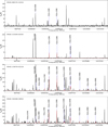 |
Fig. 1 Sample spectra of HC3N* in SPW 8 for four typical hot cores. The black lines show the observed spectra at sky frequencies, and the red lines show the XCLASS modeled spectra using the best-fit parameters for vibrationally excited HC3N lines. The complete spectra in SPW 8 for other hot cores are available in Appendix D (on Zenodo). |
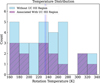 |
Fig. 2 Histogram of rotation temperatures of vibrationally excited HC3N lines observed in hot cores. The purple and sky-blue bars present the number of cores associated with and without UC HII regions. The dashed blue line indicates the average rotation temperature of 233 K for hot cores without UC HII regions, and the dashed purple line indicates the average rotation temperature of 236 K for hot cores associated with UC HII regions. |
3.3 Spatial distributions
Figure 3 shows the example moment-0 maps of 7 HC3N* states of hot cores in IRAS 16348–4654 and IRAS 18056–1952, two sources that detected the seven types of emission, for the analysis of spatial distributions of HC3N* molecules in hot cores. Because these lines selected to create moment-0 maps are not contaminated by other molecular emissions, the resulting distribution is entirely of the vibrationally exited states. The moment0 maps tentatively suggest a general similarity in the spatial distribution of various types of HC3N* emission. The emissions from different energy levels all originate from the central region of the molecular core, almost without differences in their spatial distribution. However, since these two sources are located at very large distances, we were unable to resolve the emission distribution with 3 mm data. It is also clearly that higher upper energy levels exhibit lower integrated intensities of vibrational excitation, indicating an inverse relation of the observed excitation intensity and the upper energy level. This also implies that it becomes increasingly difficult to excite higher-energy levels. Data with a higher angular resolution will reveal the actual distribution of these transitions and allow us to infer the physical and chemical properties in much greater detail. This is beyond the scope of this work, however.
Using the H40α line at 99 023 MHz from SPW 7, we identified 20 hot cores that are affected by ionized hydrogen gas emission. As shown in Fig. 4, the HC3N* molecular emission peaks and the continuum cores consistently shift in regions associated with UC HII regions. Six of the 20 hot cores with UC HII regions (I12326-6245, I6060-5146, I16076-5134, I16348-4654, I17175-3544, and I17441-2822) displayed significant separations greater than 4500 au, 11 cases (I13471-6120, I15254-5621, I15520-5234, I16065-5158, I16071-5142, I16164-5046, I16172-5028, I17016-4124, I17220-3609, I18507+0110, and I19078+0901c1) showed relatively small separations smaller than 4500 au, and 3 cases (I18032-2032c4, I18469-0132, and I19095+0930) were aligned with the H40α peak. Figure 5 illustrates the spatial distribution of HC3N* molecules in hot cores without an UC HII region. Of the hot cores without UC HII regions, 28 sources clearly exhibit consistent alignment, while only 4 sources (I13484-6100, I16344-4658, I17233-3606, and I18182-1433) show minor peak shifts, with separations smaller than 4500 au.
4 Discussion
4.1 The role of UC HII regions
The intense ultraviolet (UV) radiation and associated pressure originating from UC HII regions play a crucial role in shaping the motion and structure of the surrounding interstellar medium (Armentrout 2018). The left panel of Fig. 6 provides a histogram of the angular distances between the peaks of HC3N* and H40α emission in sources associated with UC HII regions. In hot cores associated with UC HII regions separated by less than 4500 au, UV radiation has the potential to push interstellar molecules away from the cloud core by radiation pressure. However, at larger separations, the peak shifts may be attributed to two factors. First, photodissociation of HC3N* molecules occurs due to the radiation from UC HII regions. Second, the molecular gas densities at peak positions of UC HII regions fall below the critical densities, and HC3N* cannot be stimulated effectively. These cases suggest that hot cores associated with UC HII regions might be influenced by an energy source that is distinct from the source that drives the UC HII region itself. The right panel of Fig. 6 displays a histogram of the angular distances between the peaks of HC3N* and continuum emission in sources without UC HII regions. In most hot cores without UC HII regions, where the peaks of HC3N* and continuum emissions are well aligned, the heating source is likely stars (or protostars) with luminosities below 103 L⊙, which is insufficient to generate an HII region through UV photon emission. This hypothesis is further supported by the observation that half of the cores listed in Table C.1 have masses below 50 M⊙, which is typically inadequate to form luminous protostars. In a few cases, hot cores may be heated by luminous protostars with strong UV radiation, but the appearance of an HII region is quenched by the infalling gas.
We categorized the types of hot cores based on the number of HC3N* states and refer to each category as a different excitation type (e.g., excitation type 2 means that a hot core has HC3N v7 = 1 and v7 = 2 lines, and excitation type 3 means that a hot core has HC3N v7 = 1, v7 = 2, and v6 = 1 lines.). Figure 7 illustrates the correlation between the integrated flux and the peak flux of dust associated with and without UC HII regions. After the correction for continuum flux by deducting free-free emission, hot cores with higher energy levels of excitation types tend to have higher dust flux. The ratio of the peak intensity to the integrated intensity can indicate whether a source is compact or extended. A higher ratio suggests a more compact source. The hot cores with HC3N* excitation have a strong linear relation of the peak dust flux and the integrated dust flux, indicating that these sources are relatively compact. In contrast, hot cores without HC3N* excitation or with v7 = 1 states alone have a poor linear relation, suggesting that these hot cores are not dense enough. This suggests that the excitation of HC3N* requires a dense environment.
 |
Fig. 3 Spatial distribution of 7 HC3N* lines of hot cores in IRAS 16348-4654 (top row) and IRAS 18056-1952 (bottom row). The background image of each panel from left to right is the moment-0 map of the (a) v7 = 1, Eu = 349.77530 K, (b) v7 = 2, Eu = 670.68918 & 673.96249 & 673.96308 K, (c) v6 = 1, Eu = 746.53960 K, Eu = 1065.29153 & 1066.4191 K, (d) v5 = 1 Eu = 983.03920 K, (e) v7 = 3, Eu = 990.39731 K, (f) v6 = v7 = 1, and (g) v4 = 1, Eu = 1274.35207 K emission. The white contours represent the intensity of the continuum emission, with contour levels ranging from 10% to 90% of the peak values in steps of 20%. The corresponding beam sizes are shown in the bottom left corner, and the linear scales are shown in the bottom right corner of the first image of each panel. |
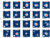 |
Fig. 4 Spatial distributions of HC3N v7 = 1 emission in 20 sources associated with UC HII regions. The background images are moment-0 maps of v7 = 1 emission. The white contours represent the intensity of continuum emission, with contour levels ranging from 10% to 90% of the peak values in steps of 20%. The red contours represent the intensity of UC HII regions (traced by H40α emission), also with contour levels ranging from 10% to 90% of the peak values in steps of 20%. The corresponding beam sizes are shown in the bottom left corner, and the linear scales are shown in the bottom right corner of the image of each source. |
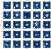 |
Fig. 5 Spatial distribution of HC3N v7 = 1 in 25 sources without UC HII regions. The background images are moment-0 maps of v7 = 1 emissions. The white contours represent the intensity of continuum emission, with contour levels ranging from 10% to 90% of the peak values in steps of 20%. The corresponding beam sizes are shown in the bottom left corner, and the linear scales are shown in the bottom right corner of the image of each source. |
4.2 Differentiation of the HC3N* column density
Excitation types 2 and 3, which have similar upper energy levels, display similar HC3N* column densities that range from (6.9 ± 0.3) × 1015 to (2.5 ± 0.1) × 1016 cm−2. Similarly, the HC3N* column density values of excitation types 5 and 6, also with comparable upper energy levels, range from (1.4 ± 0.1) × 1016 to (7.6 ± 0.1) × 1016 cm−2. In particular, the two hot cores classified as excitation type 7 exhibit the highest HC3N* column densities. They exceed 1017 cm−2. Therefore, significant differences in HC3N* column density are observed between these various types of hot cores. Figure 8 illustrates the column densities for all types of hot cores with different numbers of HC3N* states. The HC3N* column density clearly increases in general with increasing upper energy level, and hot cores with similar upper energy levels exhibit similar HC3N* column densities.
Based on these excitation types, we identify two distinguishing values of HC3N* column density: 1.9 × 1016 cm−2 and 7.6 × 1016 cm−2. The column densities of hot cores in excitation types 2 and 3 are for 92.3% below the first distinguishing value of 1.9 × 1016 cm−2. In contrast, the column densities of 92.9% of the hot cores in excitation types 5 and 6 lie between the two distinguishing values and range from 1.9 × 1016 cm−2 to 7.6 × 1016 cm−2. In all hot cores in excitation type 7, NH2 exceeds the second distinguishing value of 7.6 × 1016 cm−2. Our observations indicate that the number of vibrationally excited states increases with the overall column density of HC3N*, and higher-energy lines are more easily detected when the column density is higher.
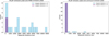 |
Fig. 6 Histogram of the separations (angular distances) between the peak of the HC3N* emission and peak of the H40α emission for sources associated with UC HII regions (left panel) and the separations between the peak of the HC3N* emission and peak of the continuum emission for sources without UC HII regions (right panel). The blue bars represent sources with angular distances greater than zero, and the purple bars represent sources with angular distances equal to zero. |
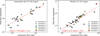 |
Fig. 7 Scatter plot of the peak flux vs. integrated flux for sources associated with UC HII regions (left panel) and for sources without UC HII regions (right panel). The different markers represent different types of hot cores that possess different numbers of HC3N* states. The linear least-squares fit for all dots is shown as the solid red line. |
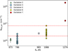 |
Fig. 8 Scatter plot of the distribution of the HC3N* column density as a function of upper level energy. The different markers represent different types of hot cores with different numbers of HC3N* emission lines. The two horizontal dashed red lines represent the two distinguishing values for the column density of 1.9 × 1016 cm−2 and 7.6 × 1016 cm−2, respectively. |
4.3 Excitation factors
The excitation of HC3N* states can be produced by two different mechanisms: pumping by the absorption of mid-IR photons, and/or collisions with H2. The strong thermal emission by hot dust, which provides high-energy mid-IR photons, can excite HC3N* from a low to a high energy level. The excitation of HC3N* states may also be impacted by the H2 number density n(H2). When n(H2) exceeds ncrit for the collision excitation of vibration levels, the excitation of a vibrationally excited state is dominated by collisions with H2. Column 11 in Tables C.1 to C.4 lists n(H2) for all sources. Figure 9 illustrates the distribution of n(H2) as a function of the upper level energy. All hot cores in our sample except for I18507+0110, for which n(H2) is lower than ncrit, indicate that excitation of HC3N* is dominated by mid-IR pumping and collisional excitation is relatively ineffective. This agrees with previous observations (Goldsmith et al. 1985; Schilke et al. 1992).
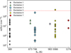 |
Fig. 9 Scatter plot of the distribution of H2 number density as a function of upper level energy. The different markers represent different types of hot cores with different numbers of HC3N* emission lines. The horizontal dashed red line represents the critical density of 4 × 108 cm−3 for HC3N v7 = 1 excitation. |
5 Conclusions
We have performed a systematic survey of vibrationally excited HC3N lines (HC3N*) in hot cores using the data of ALMA band 3 survey obtained by the ATOMS project. The main results are summarized below.
(1) Emission from seven different HC3N* states was detected in 52 out of the 60 hot cores. The detection rates for different HC3N* states decrease with increasing upper level energy. When a high-energy level line is detected in a hot core, a low-energy level line is invariably present.
(2) By analyzing the spatial distribution of HC3N v7 = 1 and UC HII regions, we found that the spatial distribution of HC3N* is influenced by the presence of UC HII regions.
(3) The derived rotation temperature for HC3N* ranges from (160 ± 1) to (335 ± 2) K, with a mean value of 235 K, and the H2 number density ranges from (1.3 ± 0.2) × 105 to (5.0 ± 0.5) × 108 cm−3, with a mean value of 3.2 × 107 cm−3. The high rotation temperature and substantial H2 number density show that HC3N* is excited from the inner region of hot cores.
(4) The column density of HC3N* ranges from (6.9 ± 0.3) × 1015 to (1.7 ± 0.1) × 1018 cm−2, with a mean value of 2.7 × 1016 cm−2. Two distinguishing values of the HC3N* column density for hot cores with different numbers of HC3N* states were obtained. Hot cores with fewer than four HC3N* states have a column density lower than 1.9 × 1016 cm−2, while those with more than six HC3N* states have a column density greater than 7.6 × 1016 cm−2. The column density of the remaining hot cores falls between these two values.
(5) In hot cores, the HC3N* states are pumped by the absorption of mid-IR photon and not by collisional excitation.
Data availability
The derived data underlying this article are available in the article and in its online supplementary material on Zenodo.
Acknowledgements
This work has been supported by the National Key R&D Program of China (No. 2022YFA1603100), the National Natural Science Foundation of China (NSFC) through grant Nos. 12033005, 12073061, and 12122307, and the Tianchi Talent Program of Xinjiang Uygur Autonomous Region. This research was carried out in part at the Jet Propulsion Laboratory, California Institute of Technology, under a contract with the National Aeronautics and Space Administration (80NM0018D0004). G.G. gratefully acknowledges support by the ANID BASAL project FB210003. M.Y.T. acknowledges the support by the NSFC through grant No. 12203011, and the Yunnan Provincial Department of Science and Technology through grant No. 202101BA070001-261. PS was partially supported by a Grant-in-Aid for Scientific Research (KAKENHI Number JP22H01271 and JP23H01221) of JSPS. PS was supported by Yoshinori Ohsumi Fund (Yoshinori Ohsumi Award for Fundamental Research). SRD acknowledges support from the Fondecyt Postdoctoral fellowship (project code 3220162) and ANID BASAL project FB210003. LB gratefully acknowledges support by the ANID BASAL project FB210003. CWL was supported by the Basic Science Research Program through the NRF funded by the Ministry of Education, Science and Technology (NRF-2019R1A2C1010851) and by the Korea Astronomy and Space Science Institute grant funded by the Korea government (MSIT; project No. 2024-1-841-00). H.-L. Liu was supported by Yunnan Fundamental Research Project (grant Nos 202301AT070118, and 202401AS070121), and by Xingdian Talent Support Plan-Youth Project. X.H.L. acknowledges support from the Natural Science Foundation of Xinjiang Uygur Autonomous Region (No. 2024D01E37) and the National Science Foundation of China (12473025). This work is sponsored in part by the Chinese Academy of Sciences (CAS), through a grant to the CAS South America Center for Astronomy (CAS-SACA) in Santiago, Chile. This paper makes use of the following ALMA data: ADS/JAO.ALMA#2019.1.00685.S. ALMA is a partnership of ESO (representing its member states), NSF (USA), and NINS (Japan), together with NRC (Canada), MOST and ASIAA (Taiwan), and KASI (Republic of Korea), in cooperation with the Republic of Chile. The Joint ALMA Observatory is operated by ESO, AUI/NRAO, and NAOJ.
Appendix A Parameters of vibrationally excited HC3N lines in SPW 8
Lowest vibrational modes of HC3N.
Appendix B Physical parameters derived from vibrationally exited HC3N lines
Table B.1 lists the detected HC3N* states in hot cores, along with their corresponding rotation temperatures and column densities.
Physical parameters derived from vibrationally exited HC3N lines.
Appendix C The basic physical parameters of hot cores
Tables C.1 to C.4 present the basic physical parameters of the hot cores. These tables categorize and list the parameters of hot cores based on whether they are associated with UC HII regions and show HC3N* emission.
Basic physical parameters of hot cores without UC HII regions which show HC3N* emission.
Basic physical parameters of hot cores without UC HII regions without HC3N* emission.
Basic physical parameters of hot cores associated with UC HII regions which show HC3N* emission.
Basic physical parameters of hot cores associated with UC HII regions without HC3N* emission.
Appendix D Spectra of vibrationally excited HC3N lines in SPW 8
In the survey observations, we detected a total of 7 types of HC3N* lines in 52 hot cores, comprising 18 transitions in SPW 8, with none detected in SPW 7, all corresponding to the same J=11 − 10 transition. Of the 52 hot cores, 29 show more than one HC3N* state, and we performed XCLASS fitting on the spectral lines. In Fig. D.1 (on Zenodo), we labeled all detected HC3N* transitions and one HC3N v=0 ground state transition.
Appendix E Rotational temperature diagram
Figure E.1 (on Zenodo) presents the RTD analysis for 29 hot cores. Since XCLASS considers the effect of optical depth on line flux, while our RTD calculations do not apply this correction, the rotation temperature derived from RTD is unreliable for optically thick sources. Of these 29 hot cores, only IRAS 18056–1952 is optically thick. For the remaining 28 hot cores, the rotation temperatures obtained from XCLASS and RTD are consistent when considering the errors.
References
- Afflerbach, A., Churchwell, E., Acord, J. M., et al. 1996, ApJS, 106, 423 [NASA ADS] [CrossRef] [Google Scholar]
- Armentrout, W. P. 2018, PhD thesis, West Virginia University, USA [Google Scholar]
- Belloche, A., Müller, H. S. P., Menten, K. M., Schilke, P., & Comito, C. 2013, A&A, 559, A47 [NASA ADS] [CrossRef] [EDP Sciences] [Google Scholar]
- Bergin, E. A., Snell, R. L., & Goldsmith, P. F. 1996, ApJ, 460, 343 [NASA ADS] [CrossRef] [Google Scholar]
- Bonfand, M., Belloche, A., Garrod, R. T., et al. 2019, A&A, 628, A27 [NASA ADS] [CrossRef] [EDP Sciences] [Google Scholar]
- Bonfand, M., Csengeri, T., Bontemps, S., et al. 2024, A&A, 687, A163 [NASA ADS] [CrossRef] [EDP Sciences] [Google Scholar]
- CASA Team (Bean, B., et al.) 2022, PASP, 134, 114501 [NASA ADS] [CrossRef] [Google Scholar]
- Chung, H. S., Osamu, K., & Masaki, M. 1991, J. Korean Astron. Soc., 24, 217 [NASA ADS] [Google Scholar]
- Churchwell, E. 2002, ARA&A, 40, 27 [Google Scholar]
- Condon, J. J., & Ransom, S. M. 2016, Essential Radio Astronomy (Princeton, NJ: Princeton University Press) [Google Scholar]
- Costagliola, F., & Aalto, S. 2010, A&A, 515, A71 [NASA ADS] [CrossRef] [EDP Sciences] [Google Scholar]
- de Vicente, P., Martín-Pintado, J., Neri, R., & Colom, P. 2000, A&A, 361, 1058 [NASA ADS] [Google Scholar]
- Endres, C. P., Schlemmer, S., Schilke, P., Stutzki, J., & Müller, H. S. P. 2016, J. Mol. Spectrosc., 327, 95 [NASA ADS] [CrossRef] [Google Scholar]
- Esplugues, G. B., Cernicharo, J., Viti, S., et al. 2013, A&A, 559, A51 [NASA ADS] [CrossRef] [EDP Sciences] [Google Scholar]
- Frau, P., Girart, J. M., Beltrán, M. T., et al. 2010, ApJ, 723, 1665 [Google Scholar]
- Gerin, M., Neufeld, D. A., & Goicoechea, J. R. 2016, ARA&A, 54, 181 [NASA ADS] [CrossRef] [Google Scholar]
- Giannetti, A., Leurini, S., König, C., et al. 2017, A&A, 606, L12 [NASA ADS] [CrossRef] [EDP Sciences] [Google Scholar]
- Goldsmith, P. F., & Langer, W. D. 1999, ApJ, 517, 209 [Google Scholar]
- Goldsmith, P. F., Snell, R. L., Deguchi, S., Krotkov, R., & Linke, R. A. 1982, ApJ, 260, 147 [Google Scholar]
- Goldsmith, P. F., Krotkov, R., & Snell, R. L. 1985, ApJ, 299, 405 [Google Scholar]
- He, Y.-X., Henkel, C., Zhou, J.-J., et al. 2021, ApJS, 253, 2 [NASA ADS] [CrossRef] [Google Scholar]
- Herbst, E., & van Dishoeck, E. F. 2009, ARA&A, 47, 427 [NASA ADS] [CrossRef] [Google Scholar]
- Hildebrand, R. H. 1983, QJRAS, 24, 267 [NASA ADS] [Google Scholar]
- Jørgensen, J. K., Belloche, A., & Garrod, R. T. 2020, ARA&A, 58, 727 [Google Scholar]
- Kauffmann, J., Bertoldi, F., Bourke, T. L., Evans, N. J., I., & Lee, C. W. 2008, A&A, 487, 993 [NASA ADS] [CrossRef] [EDP Sciences] [Google Scholar]
- Khan, S., Pandian, J. D., Lal, D. V., et al. 2022, A&A, 664, A140 [NASA ADS] [CrossRef] [EDP Sciences] [Google Scholar]
- Kunde, V. G., Aikin, A. C., Hanel, R. A., et al. 1981, Nature, 292, 686 [NASA ADS] [CrossRef] [Google Scholar]
- Leach, S., Garcia, G. A., Mahjoub, A., et al. 2014, J. Chem. Phys., 140, 174305 [NASA ADS] [CrossRef] [Google Scholar]
- Li, D., & Goldsmith, P. F. 2012, ApJ, 756, 12 [NASA ADS] [CrossRef] [Google Scholar]
- Li, S., Wang, J., Zhang, Z.-Y., et al. 2017, MNRAS, 466, 248 [NASA ADS] [CrossRef] [Google Scholar]
- Liu, T., Evans, N. J., Kim, K.-T., et al. 2020, MNRAS, 496, 2790 [Google Scholar]
- Liu, H.-L., Liu, T., Evans, Neal J., I., et al. 2021, MNRAS, 505, 2801 [NASA ADS] [CrossRef] [Google Scholar]
- Liu, X., Liu, T., Shen, Z., et al. 2024, ApJS, 271, 3 [NASA ADS] [CrossRef] [Google Scholar]
- Lu, X., Cheng, Y., Ginsburg, A., et al. 2020, ApJ, 894, L14 [NASA ADS] [CrossRef] [Google Scholar]
- Luo, A.-X., Liu, H.-L., Li, G.-X., Pan, S., & Yang, D.-T. 2024, Res. Astron. Astrophys., 24, 065003 [CrossRef] [Google Scholar]
- Mallinson, P. D., & Fayt, A. 1976, Mol. Phys., 32, 473 [NASA ADS] [CrossRef] [Google Scholar]
- Martín, S., Mangum, J. G., Harada, N., et al. 2021, A&A, 656, A46 [NASA ADS] [CrossRef] [EDP Sciences] [Google Scholar]
- Mauersberger, R., Henkel, C., & Sage, L. J. 1990, A&A, 236, 63 [NASA ADS] [Google Scholar]
- McMullin, J. P., Waters, B., Schiebel, D., Young, W., & Golap, K. 2007, in Astronomical Society of the Pacific Conference Series Analysis Software and Systems XVI, eds. R. A. Shaw, F. Hill, & D. J. Bell, 127 [Google Scholar]
- Möller, T., Endres, C., & Schilke, P. 2017, A&A, 598, A7 [NASA ADS] [CrossRef] [EDP Sciences] [Google Scholar]
- Motte, F., Bontemps, S., & Louvet, F. 2018, ARA&A, 56, 41 [NASA ADS] [CrossRef] [Google Scholar]
- Müller, H. S. P., Thorwirth, S., Roth, D. A., & Winnewisser, G. 2001, A&A, 370, L49 [Google Scholar]
- Müller, H. S. P., Schlöder, F., Stutzki, J., & Winnewisser, G. 2005, J. Mol. Struct., 742, 215 [Google Scholar]
- Ossenkopf, V., & Henning, T. 1994, A&A, 291, 943 [NASA ADS] [Google Scholar]
- Pagani, L., Favre, C., Goldsmith, P. F., et al. 2017, A&A, 604, A32 [NASA ADS] [CrossRef] [EDP Sciences] [Google Scholar]
- Peng, Y., Qin, S.-L., Schilke, P., et al. 2017, ApJ, 837, 49 [NASA ADS] [CrossRef] [Google Scholar]
- Pickett, H. M., Poynter, R. L., Cohen, E. A., et al. 1998, J. Quant. Spec. Radiat. Transf., 60, 883 [Google Scholar]
- Qin, S.-L., Liu, T., Liu, X., et al. 2022, MNRAS, 511, 3463 [CrossRef] [Google Scholar]
- Ranković, M., Nag, P., Zawadzki, M., et al. 2018, Phys. Rev. A, 98, 052708 [CrossRef] [Google Scholar]
- Rico-Villas, F., Martín-Pintado, J., González-Alfonso, E., Martín, S., & Rivilla, V. M. 2020, MNRAS, 491, 4573 [NASA ADS] [CrossRef] [Google Scholar]
- Rico-Villas, F., Martín-Pintado, J., González-Alfonso, E., et al. 2021, MNRAS, 502, 3021 [NASA ADS] [CrossRef] [Google Scholar]
- Rosen, A. L. 2022, ApJ, 941, 202 [NASA ADS] [CrossRef] [Google Scholar]
- Saha, A., Tej, A., Liu, H.-L., et al. 2022, MNRAS, 516, 1983 [NASA ADS] [CrossRef] [Google Scholar]
- Schilke, P., Guesten, R., Schulz, A., Serabyn, E., & Walmsley, C. M. 1992, A&A, 261, L5 [Google Scholar]
- Shaver, P. A. 1970, Astrophys. Lett., 5, 167 [NASA ADS] [Google Scholar]
- Tang, M., Liu, T., Qin, S.-L., et al. 2018, ApJ, 856, 141 [NASA ADS] [CrossRef] [Google Scholar]
- Taniguchi, K., Saito, M., Sridharan, T. K., & Minamidani, T. 2018, ApJ, 854, 133 [NASA ADS] [CrossRef] [Google Scholar]
- Taniguchi, K., Tanaka, K. E. I., Zhang, Y., et al. 2022, ApJ, 931, 99 [CrossRef] [Google Scholar]
- Taniguchi, K., Sanhueza, P., Olguin, F. A., et al. 2023, ApJ, 950, 57 [CrossRef] [Google Scholar]
- Thorwirth, S., Müller, H. S. P., & Winnewisser, G. 2000, J. Mol. Spectrosc., 204, 133 [NASA ADS] [CrossRef] [Google Scholar]
- Turner, B. E. 1971, ApJ, 163, L35 [NASA ADS] [CrossRef] [Google Scholar]
- van Dishoeck, E. F. 2018, in IAU Symposium, 332, Astrochemistry VII: Through the Cosmos from Galaxies to Planets, eds. M. Cunningham, T. Millar, & Y. Aikawa, 3 [Google Scholar]
- Velilla Prieto, L., Sánchez Contreras, C., Cernicharo, J., et al. 2015, A&A, 575, A84 [CrossRef] [EDP Sciences] [Google Scholar]
- Wang, J., Li, D., Goldsmith, P. F., et al. 2020, ApJ, 889, 129 [NASA ADS] [CrossRef] [Google Scholar]
- Wyrowski, F., Schilke, P., & Walmsley, C. M. 1999, A&A, 341, 882 [NASA ADS] [Google Scholar]
- Yamada, K. M. T., & Creswell, R. A. 1986, J. Mol. Spectrosc., 116, 384 [NASA ADS] [CrossRef] [Google Scholar]
- Yu, N., Wang, J.-J., & Xu, J.-L. 2019, MNRAS, 489, 4497 [CrossRef] [Google Scholar]
- Yue, Y.-H., Qin, S.-L., Liu, T., et al. 2021, Res. Astron. Astrophys., 21, 014 [CrossRef] [Google Scholar]
- Zhang, C.-P., & Li, G.-X. 2017, MNRAS, 469, 2286 [Google Scholar]
- Zinchenko, I. I., Dewangan, L. K., Baug, T., Ojha, D. K., & Bhadari, N. K. 2021, MNRAS, 506, L45 [NASA ADS] [CrossRef] [Google Scholar]
All Tables
Basic physical parameters of hot cores without UC HII regions which show HC3N* emission.
Basic physical parameters of hot cores without UC HII regions without HC3N* emission.
Basic physical parameters of hot cores associated with UC HII regions which show HC3N* emission.
Basic physical parameters of hot cores associated with UC HII regions without HC3N* emission.
All Figures
|
Fig. 1 Sample spectra of HC3N* in SPW 8 for four typical hot cores. The black lines show the observed spectra at sky frequencies, and the red lines show the XCLASS modeled spectra using the best-fit parameters for vibrationally excited HC3N lines. The complete spectra in SPW 8 for other hot cores are available in Appendix D (on Zenodo). |
| In the text | |
|
Fig. 2 Histogram of rotation temperatures of vibrationally excited HC3N lines observed in hot cores. The purple and sky-blue bars present the number of cores associated with and without UC HII regions. The dashed blue line indicates the average rotation temperature of 233 K for hot cores without UC HII regions, and the dashed purple line indicates the average rotation temperature of 236 K for hot cores associated with UC HII regions. |
| In the text | |
|
Fig. 3 Spatial distribution of 7 HC3N* lines of hot cores in IRAS 16348-4654 (top row) and IRAS 18056-1952 (bottom row). The background image of each panel from left to right is the moment-0 map of the (a) v7 = 1, Eu = 349.77530 K, (b) v7 = 2, Eu = 670.68918 & 673.96249 & 673.96308 K, (c) v6 = 1, Eu = 746.53960 K, Eu = 1065.29153 & 1066.4191 K, (d) v5 = 1 Eu = 983.03920 K, (e) v7 = 3, Eu = 990.39731 K, (f) v6 = v7 = 1, and (g) v4 = 1, Eu = 1274.35207 K emission. The white contours represent the intensity of the continuum emission, with contour levels ranging from 10% to 90% of the peak values in steps of 20%. The corresponding beam sizes are shown in the bottom left corner, and the linear scales are shown in the bottom right corner of the first image of each panel. |
| In the text | |
|
Fig. 4 Spatial distributions of HC3N v7 = 1 emission in 20 sources associated with UC HII regions. The background images are moment-0 maps of v7 = 1 emission. The white contours represent the intensity of continuum emission, with contour levels ranging from 10% to 90% of the peak values in steps of 20%. The red contours represent the intensity of UC HII regions (traced by H40α emission), also with contour levels ranging from 10% to 90% of the peak values in steps of 20%. The corresponding beam sizes are shown in the bottom left corner, and the linear scales are shown in the bottom right corner of the image of each source. |
| In the text | |
|
Fig. 5 Spatial distribution of HC3N v7 = 1 in 25 sources without UC HII regions. The background images are moment-0 maps of v7 = 1 emissions. The white contours represent the intensity of continuum emission, with contour levels ranging from 10% to 90% of the peak values in steps of 20%. The corresponding beam sizes are shown in the bottom left corner, and the linear scales are shown in the bottom right corner of the image of each source. |
| In the text | |
|
Fig. 6 Histogram of the separations (angular distances) between the peak of the HC3N* emission and peak of the H40α emission for sources associated with UC HII regions (left panel) and the separations between the peak of the HC3N* emission and peak of the continuum emission for sources without UC HII regions (right panel). The blue bars represent sources with angular distances greater than zero, and the purple bars represent sources with angular distances equal to zero. |
| In the text | |
|
Fig. 7 Scatter plot of the peak flux vs. integrated flux for sources associated with UC HII regions (left panel) and for sources without UC HII regions (right panel). The different markers represent different types of hot cores that possess different numbers of HC3N* states. The linear least-squares fit for all dots is shown as the solid red line. |
| In the text | |
|
Fig. 8 Scatter plot of the distribution of the HC3N* column density as a function of upper level energy. The different markers represent different types of hot cores with different numbers of HC3N* emission lines. The two horizontal dashed red lines represent the two distinguishing values for the column density of 1.9 × 1016 cm−2 and 7.6 × 1016 cm−2, respectively. |
| In the text | |
|
Fig. 9 Scatter plot of the distribution of H2 number density as a function of upper level energy. The different markers represent different types of hot cores with different numbers of HC3N* emission lines. The horizontal dashed red line represents the critical density of 4 × 108 cm−3 for HC3N v7 = 1 excitation. |
| In the text | |
Current usage metrics show cumulative count of Article Views (full-text article views including HTML views, PDF and ePub downloads, according to the available data) and Abstracts Views on Vision4Press platform.
Data correspond to usage on the plateform after 2015. The current usage metrics is available 48-96 hours after online publication and is updated daily on week days.
Initial download of the metrics may take a while.