| Issue |
A&A
Volume 694, February 2025
|
|
|---|---|---|
| Article Number | A115 | |
| Number of page(s) | 16 | |
| Section | Cosmology (including clusters of galaxies) | |
| DOI | https://doi.org/10.1051/0004-6361/202452396 | |
| Published online | 07 February 2025 | |
Cooling rate and turbulence in the intracluster medium of the cool-core cluster Abell 2667
1
INAF-Osservatorio Astrofisico di Arcetri, Largo Enrico Fermi 5, 50125 Firenze, Italy
2
Dipartimento di Fisica e Astronomia, Università degli Studi di Firenze, Via Sansone, 1, 50019 Sesto Fiorentino, Firenze, Italy
3
INAF – IASF Palermo, Via Ugo La Malfa 153, 80146 Palermo, Italy
4
Department of Physics, Informatics and Mathematics, University of Modena and Reggio Emilia, 41125 Modena, Italy
5
INAF-IASF Milano, Via A. Corti 12, I-20133 Milano, Italy
6
Max Planck Institute for Extraterrestrial Physics, Giessenbachstrasse 1, 85748 Garching, Germany
7
Institute for Frontiers in Astronomy and Astrophysics, Beijing Normal University, Beijing 102206, China
8
Dipartimento di Fisica e Scienze della Terra, Università degli Studi di Ferrara, Via Saragat 1, I-44122 Ferrara, Italy
9
University of Leiden, Rapenburg 70, 2311 EZ Leiden, The Netherlands
10
Kapteyn Astronomical Institute, University of Groningen, PO Box 800 9700 AV Groningen, The Netherlands
11
Department of Physics and Astronomy, Università degli Studi di Padova, Vicolo dell’Osservatorio 3, I-35122 Padova, Italy
12
INAF – Osservatorio Astronomico di Padova, Vicolo dell’Osservatorio 5, I-35122 Padova, Italy
⋆ Corresponding author; This email address is being protected from spambots. You need JavaScript enabled to view it.
Received:
27
September
2024
Accepted:
29
December
2024
Abstract
Context. We present a detailed analysis of the thermal X-ray emission from the intracluster medium in the cool-core galaxy cluster Abell 2667 at z = 0.23.
Aims. Our main goal is to detect low-temperature (< 2 keV) X-ray emitting gas associated with a potential cooling flow connecting the hot intracluster medium reservoir to the cold gas phase responsible for star formation and supermassive black hole feeding.
Methods. We combined new deep XMM-Newton EPIC and RGS data, along with archival Chandra data, and performed a spectral analysis of the emission from the core region.
Results. We find 1σ upper limits on the fraction of gas cooling equal to ∼40 M⊙ yr−1 and ∼50−60 M⊙ yr−1, in the temperature ranges of 0.5−1 keV and 1−2 keV, respectively. We do not identify OVII, FeXXI-FeXXII, and FeXVII recombination and resonant emission lines in our RGS spectra, implying that the fraction of gas cooling below 1 keV is limited to a few tens of solar masses per year at maximum. We do detect several lines (particularly SiXIV, MgXII, FeXXIII/FeXXIV, NeX, OVIIIα) from which we are able to estimate the turbulent broadening. We obtain a 1σ upper limit of ∼320 km/s, which is much higher than the one found in other cool-core clusters such as Abell 1835, suggesting the presence of some mechanisms that boost significant turbulence in the atmosphere of Abell 2667. Imaging analysis of Chandra data suggests the presence of a cold front possibly associated with sloshing or with intracluster medium cavities. However, current data do not allow us to clearly identify the dominant physical mechanism responsible for turbulence.
Conclusions. These findings show that Abell 2667 is not different from other, low-redshift, cool-core clusters, with only upper limits on the mass deposition rate associated with possible isobaric cooling flows. Despite the lack of clear signatures of recent feedback events, the large upper limit on the turbulent velocity leaves room for significant heating of the intracluster medium, which may quench cooling in the cool core for an extended period, albeit also driving local intracluster medium fluctuations that will contribute to the next cycle of condensation rain.
Key words: galaxies: clusters: general / galaxies: clusters: intracluster medium / galaxies: clusters: individual: Abell 2667 / X-rays: galaxies: clusters
© The Authors 2025
 Open Access article, published by EDP Sciences, under the terms of the Creative Commons Attribution License (https://creativecommons.org/licenses/by/4.0), which permits unrestricted use, distribution, and reproduction in any medium, provided the original work is properly cited.
This article is published in open access under the Subscribe to Open model. This email address is being protected from spambots. You need JavaScript enabled to view it. to support open access publication.
1. Introduction
Galaxy clusters are the largest gravitationally bound structures in the Universe. These are formed by baryonic and nonbaryonic matter in different states and with different assembly histories. Typically they host 100−1000 galaxies in virial equilibrium with a total halo mass varying between 1014 M⊙ and 1015 M⊙ and a diameter of a few megaparsecs. The stellar mass in member galaxies typically amounts to 2−5% only of the total observed mass. The majority of the mass of the halo is contributed by dark matter, with a mass fraction of ∼0.8. Most of the remaining mass budget (15−18%) is contributed by a tenuous, high-temperature (∼107 − 108 K) plasma with a typical electron density on the order of 10−3 cm−3: the intracluster medium (ICM). The ICM is expected to be in an approximate hydrostatic equilibrium in the cluster potential well and can be detected in the X-ray band thanks to its thermal bremsstrahlung emission plus line emission from heavy element ions.
In some clusters, the ICM density profile can be described by a single β model (Cavaliere & Fusco-Femiano 1978) that is rapidly decreasing with radius toward the outskirts outside a flat core. This description, however, is not accurate for many clusters that show sharply peaked profiles, dubbed cool cores, which can reach electron densities as high as 0.1 cm−3 in the center. In these cases, a double β model is required, suggesting that physical processes acting in the core are modifying the ICM distribution. This is not surprising, since the gas cooling time, which scales as the inverse of the density, is measured to be much shorter than the Hubble time in cool cores (McNamara et al. 2005; Fabian et al. 2006; Vantyghem et al. 2014; Sanders et al. 2014) over a fairly large redshift interval (Santos et al. 2010).
This initially led to the conclusion that a massive cooling flow (CF) is developing in the ICM of most clusters with cool cores (Fabian & Nulsen 1977). According to the original isobaric CF scenario (Fabian 1994), the gas in the central regions of clusters should experience adiabatic compression at constant pressure, cooling mainly through X-ray emission, and inevitably condensate into clouds of cold gas. This picture is supported by the observation of temperature drops toward the center (McNamara et al. 2000; Tamura et al. 2001; Sanders & Fabian 2007; Cavagnolo et al. 2009; Sonkamble et al. 2024; Liu et al. 2024). In addition, the emission measure of the ICM as a function of temperature can be accurately predicted in the framework of the adiabatic CF model, and therefore the associated mass deposition rates (MDRs) can be directly inferred by the spectral distribution of the X-ray emission from the cool core. The MDR values based on the isobaric CF model and estimated from the total core luminosity are typically estimated to be in the range of 100−1000 M⊙ yr−1. However, the bulk of the X-ray emission is contributed by the relatively hot ICM, while the contribution from the coldest, X-ray emitting gas amounts to a few percent of the total luminosity. Typically, the cooling gas is not directly observed in CCD spectra.
Since the ICM is enriched with heavy ions, whose abundance is even higher toward the center, another key prediction of the isobaric CF model is the presence of a line-rich X-ray spectrum due to the presence of many transitions in the ionized heavy elements, which can be observed in high-resolution X-ray grating spectroscopy. Surprisingly, the analysis of the first high-resolution X-ray spectra, mostly thanks to XMM-Newton observations, clearly ruled out the isobaric CF model (the so-called soft CF problem; see Peterson et al. 2001; Molendi & Pizzolato 2001; Kaastra et al. 2001; Xu et al. 2002; Ettori et al. 2002), due to the lack of emission lines associated with gas colder than about one third of the virial value (Donahue & Voit 2004) in any cool-core clusters. Since it is extremely unlikely that the coldest gas is systematically poor in metals, the lack of emission lines directly implies the lack of the low-temperature gas predicted by the isobaric cooling model.
Given the quality of current high-resolution X-ray spectra, the presence of CFs is not completely ruled out, but they are constrained to be more than one order of magnitude lower than the ones predicted in the isobaric CF model. In addition, the maximum MDRs allowed by current data are at least one order of magnitude lower than the star formation rates (SFRs) observed in the hosted brightest cluster galaxy (BCG; Molendi et al. 2016), implying a significant difference between the timescale of cold gas consumption and the timescale of gas cooling. To date, the only convincing CF candidate is the well-documented Phoenix cluster at z ∼ 0.6 (see McDonald et al. 2012, 2019; Tozzi et al. 2015; Pinto et al. 2018). This cluster exhibits a starburst of 500−800 M⊙ yr−1 (McDonald et al. 2015; Mittal et al. 2017), comparable to a cooling rate of  M⊙ yr−1 below 2 keV (uncertainties at a 90% confidence level) measured with XMM-Newton Reflection Grating Spectrometer (RGS) data (Pinto et al. 2018; see also Tozzi et al. 2015, which found
  M⊙ yr−1 below 3 keV from RGS data).
Given the difficulty in measuring MDRs, it is not possible to firmly identify the clusters of galaxies actually hosting a CF. Phenomenologically, galaxy clusters are classified as cool-core (CC; relaxed systems with a peak in the surface brightness and mostly with regular and spheroidal shapes) and non-cool-core (NCC; systems with no bright cores typically with disturbed morphologies likely associated with ongoing merging processes; Molendi & Pizzolato 2001; Hudson et al. 2010; Zhang et al. 2016). On a general basis, CFs are expected to be hosted only by CC clusters, but their occurrence and magnitude are not quantified, and we do not have information about their duty cycle.
The inadequacy of the isobaric CF model inevitably raises the question of the mechanism preventing the gas from cooling in adiabatic mode. As of today, there is a large consensus on the heating from mechanical feedback and turbulence, mostly provided by the central active galactic nucleus (AGN; e.g., McNamara & Nulsen 2007; Fabian 2012; McKinley et al. 2022). High-resolution hydrodynamical simulations show that AGN jets or outflows can inject a sufficient amount of energy into the ICM to offset both the global cooling rates (Gaspari et al. 2012) and the differential luminosity distribution toward the soft X-ray via nonisobaric modes (Gaspari 2015). The AGN jet feedback is also crucial to stir up the ICM “weather” with substantial enstrophy (magnitude of vorticity) in the cluster cores (Wittor & Gaspari 2020, 2023). This feedback mechanism has been directly observed in many systems, such as nearby clusters, Perseus (Fabian et al. 2003, 2011), Hydra A (McNamara et al. 2000; Timmerman et al. 2022), Virgo (Werner et al. 2012; Russell et al. 2015), and Abell 2626 (Kadam et al. 2019). On the other hand, residual star formation in the BCG, the presence of cold and multiphase gas surrounding BCGs observed with ALMA (e.g., North et al. 2021) and MUSE (e.g., Maccagni et al. 2021; Olivares et al. 2022), and the distribution of heavy elements in the hot gas (e.g., Liu et al. 2019a, 2020; Gastaldello et al. 2021), suggest that at least some fraction of the hot ICM underwent cooling at some point during the secular evolution of clusters. The key point is that, to agree with current observations, CFs should be hidden, characterized by very low MDRs, or occurring on short timescales. Some recent works show that a substantial fraction of the cooling gas may be intrinsically absorbed (Fabian et al. 2022), interpreting the observed far-infrared (FIR) luminosity from the core as a consequence of the cooling rate whose emission is reprocessed by the surrounding medium. In addition, mechanical AGN feedback can stimulate the condensation of the hot phase via turbulent nonlinear thermal instability, leading to a rain of clouds or filaments that are expected to boost the SMBH feeding rate via chaotic cold accretion (CCA; Gaspari et al. 2020, for a review), characterized by a highly variable MDR. Finally, massive, short-lived CFs may occur and replenish the cold gas reservoir before being quenched by feedback processes from the central SMBH in the BCG. In every scenario, the central AGN is expected to play a key role in regulating the thermodynamics in the ICM, while shaping the hot halo properties (Pasini et al. 2021) and SMBH scaling relations (Gaspari et al. 2019).
One of the crucial open questions is how much gas cools and trickles below 1.0 keV, down to the lowest temperatures detectable in the X-ray grating spectra (0.3 − 0.5 keV). In this work, we reconsider this question using X-ray images and spectra taken with XMM European Photon Imaging Camera (EPIC), XMM/RGS and Chandra Advanced CCD Imaging Spectrometer (ACIS) of the CC cluster Abell 2667 (hereafter A2667). This cluster has a BCG with prominent ongoing activity with peculiar features such as blue and red wings, broadening of the lines, and offsets with respect to the BCG reference system, suggesting the presence of multiple gas components on scales of a few tens of kiloparsecs. It also shows a prominent AGN signature in the optical, radio, and X-ray bands, with a strongly absorbed X-ray nuclear emission (∼3 × 1043 erg s−1), and diffuse ICM emission on the order of 3 × 1045 erg s−1, comparable to that of the Phoenix cluster (McDonald et al. 2012). The similarity of the environmental properties with the Phoenix is at variance with the large difference in the strength of the activity: the nuclear emission is ∼100 and 20 times lower in A2667 in the X-ray and radio band (van Weeren et al. 2014), respectively, and the total SFR in the BCG is a factor of ∼50 lower. This composite picture makes the BCG of A2667 an interesting candidate in which to study the cooling and heating processes in clusters.
This paper is structured as follows. In Sect. 2, we describe the previous results for A2667 available in the literature. In Sect. 3, we describe the archival Chandra data. In Sect. 4, we describe the new XMM-EPIC and RGS deep observation used in this work. In Sects. 5, 6, and 7 we describe XMM-EPIC and XMM-RGS data analysis and results. In Sect. 8, we discuss the results obtained from our analysis, while in Sect. 9 we comment on the possible extension of this study with future X-ray facilities. Finally, our conclusions are summarized in Sect. 10. Throughout this paper, we adopt the current Planck cosmology with Ωm = 0.315, and H0 = 67.4 km s−1 Mpc−1 in a flat geometry (Planck Collaboration VI 2020). In this cosmology, at z = 0.23, 1 arcsec corresponds to 3.81 kpc, and the Universe is 11.01 Gyr old. Quoted error bars correspond to a 1σ confidence level, unless otherwise stated.
2. A2667: Previous observations and main results
A2667 is a lensing galaxy cluster in the nearby Universe (z = 0.233). It has multiple image systems, including one of the brightest giant gravitational arcs with an elongation of ∼10 arcsec at z = 1.0334 (Covone et al. 2006a,b). It is also associated with a radio minihalo (Giacintucci et al. 2017; Knowles et al. 2022) with a largest angular size of 4.6′ and a largest physical linear size at the cluster redshift of 1.02 Mpc (Knowles et al. 2022). This cluster is among the top 5% most luminous X-ray clusters observed in the ROSAT All Sky Survey, with a luminosity of LX = (13.39 ± 0.25)×1044 erg/s in the range of [0.1−2.4] keV within r500 = 1.38 ± 0.07 Mpc (Mantz et al. 2016). It is classified as a relaxed cluster (Gilmour et al. 2009; Kale et al. 2015; Mann & Ebeling 2012) with a BCG at the center (RA = 23:51:39.40 Dec = −26:05:03.3). The BCG hosts an X-ray AGN with intrinsic absorption NH(1022 cm−2) =  and X-ray luminosity
 ![Mathematical equation: $ \log(L_\mathrm{X[2{-}10]\,keV})[\mathrm{erg/s}]=43.4^{+0.2}_{-0.4} $](/articles/aa/full_html/2025/02/aa52396-24/aa52396-24-eq4.gif) (Yang et al. 2018). The BCG has a stellar mass of log(Mbulge/M⊙) = 11.97 ± 0.04 and hosts a SMBH whose mass is estimated to be log(MBH/M⊙) = 10.35 ± 0.27 (Phipps et al. 2019) from the standard fundamental plane relation (Merloni et al. 2003).
(Yang et al. 2018). The BCG has a stellar mass of log(Mbulge/M⊙) = 11.97 ± 0.04 and hosts a SMBH whose mass is estimated to be log(MBH/M⊙) = 10.35 ± 0.27 (Phipps et al. 2019) from the standard fundamental plane relation (Merloni et al. 2003).
The SFR in the BCG has been estimated to range between SFR = 8.7 ± 0.2 M⊙ yr−1 (via the spectral energy distribution from the FIR Spitzer and Herschel data; Rawle et al. 2012) and ≃55 M⊙ yr−1 (via MUSE spectra; Iani et al. 2019). The difference between the two estimates is a consequence of the methodologies applied and they can be considered as lower and upper limits, respectively. In effect, while the value inferred from the FIR does not take into account the contribution from unobscured star formation, the estimate by Iani et al. (2019) may be contaminated by the AGN emission. The star formation is responsible for previously noticed strong Hα and [OII]λ3727 Å lines (Rizza et al. 1998), which are often associated with CCs.
The bidimensional modeling of the BCG optical surface brightness profile reveals the presence of a complex system of substructures extending all around the galaxy. Clumps of different sizes and shapes plunged into a more diffuse component constitute these substructures, whose intense “blue” optical color hints at the presence of a young stellar population (Iani et al. 2019). However, A2667’s central region seems to be dominated by an evolved and passively aging stellar population (Covone et al. 2006a).
In the radio band, Kale et al. (2015) classified this central galaxy as a radio-loud AGN with a radio power of P = 3.16 × 1024 W Hz−1, using the National Radio Astronomy Observatory (NRAO) VLA Sky Survey radio data at 1.4 GHz. The X-ray morphology (Rizza et al. 1998) and dynamical analysis (Covone et al. 2006a) support the idea that A2667’s inner core is relaxed and shows a drop in the ICM temperature profile in the central 100 kpc, suggesting that the cluster hosts a CC with an average cooling time of ∼0.5 Gyr (Cavagnolo et al. 2009). Indeed, Zhang et al. (2016) classified this luminous cluster as a strong CC system with  .
.
3. Chandra: Observations and data reduction
Before proceeding with the reduction and analysis of our deep XMM-Newton observation, we revisited the shallow Chandra data available on the archive, provided with the highest spatial resolution, in particular to compute a Chandra soft band image (0.5−2 keV) and compute the surface brightness profile, which is necessary to model the (instrumental) line broadening expected in the RGS spectra.
A2667 was observed for 10 ks with ACIS-S granted in Cycle 02 (PI: S. Allen). The observations were completed in June 2001 with a single pointing. We performed data reduction starting from the level = 1 event files with CIAO 4.13, with the latest release of the Chandra Calibration Database at the time of writing (CALDB 4.9.4). We ran the task destreak to flag and remove spurious events (with moderate to small pulse heights) along single rows. We ran the tool acis_detect_afterglow to flag residual charge from cosmic rays in CCD pixels. Finally, as this observation is taken in the VFAINT mode, we ran the task acis_process_events with the parameter apply_cti=yes to flag background events that are most likely associated with cosmic rays and reject them. With this procedure, the ACIS particle background can be significantly reduced compared to the standard grade selection. The data were then filtered to include only the standard event grades 0, 2, 3, 4, and 6. The level 2 event files generated in this way were visually inspected for flickering pixels or hot columns left after the standard reduction but we found none after filtering out bad events. We also carefully inspected the image of the removed photons, particularly to verify whether we have pile-up effects1. Finally, time intervals with high background were filtered by performing a 3σ clipping of the background level. The light curves were extracted in the 2.3−7.3 keV band and binned with a time interval of 200 s. The time intervals when the background exceeds the average value by 3σ were removed with the tool deflare. The final total exposure time after data reduction and excluding the dead-time correction amounts to 9.6 ks (corresponding to the LIVETIME keyword in the header of Chandra fits files). Images were created in the 0.5−2 keV, 2−7 keV, and total (0.5−7 keV) bands, with no binning to preserve the full angular resolution of ∼1 arcsec (FWHM) at the aimpoint (1 pixel corresponds to 0.492 arcsec). In the left panel of Fig. 1 we show the total Chandra image.
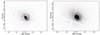 |
Fig. 1. Chandra and XMM images of A2667’s central region. Left panel: Chandra [0.3−10 keV] image of A2667 in a FoV of ∼6 × 4 arcmin2. Right panel: XMM-Newton/EPIC MOS1+MOS2+pn [0.5−7 keV] image of A2667 in a FoV of ∼6 × 4 arcmin2. The magenta circle in both images shows the spectral extraction region of 0.5 arcmin radius used in XMM/EPIC data analysis. |
4. XMM-Newton: Observations and data reduction
4.1. XMM-Newton: EPIC data
We obtained a total of 274 ks with XMM-Newton on A2667 in AO23 (Proposal ID 90028, PI: P. Tozzi). Data were acquired in December and June 2022 (see Table 1 for exposure times obtained after data reduction). To these new observations, we also added to our analysis the archival observation ObsID 0148990101 taken in 2003 (Proposal ID 14899, PI: S. Allen).
XMM-Newton data: Total exposure times obtained for each ObsID after data reduction.
The observation data files (ODFs) were processed to produce calibrated event files using the most recent release of the XMM-Newton Science Analysis System (SAS v21.0.0), with the calibration release XMM-CCF-REL-323, and running the tasks epproc and emproc for the pn and MOS, respectively, to generate calibrated and concatenated EPIC event lists. Then, we filtered EPIC event lists for bad pixels, bad columns, cosmic-ray events outside the field of view (FoV), photons in the gaps (FLAG = 0), and applied standard grade selection, corresponding to PATTERN < 12 for MOS and PATTERN ≤ 4 for pn. We removed soft proton flares by applying a threshold on the count rate in the 10−12 keV energy band. To define low-background intervals, we used the condition RATE ≤ 0.35 for MOS and RATE ≤ 0.4 for pn2. For each ObsID, we removed out-of-time (OoT) events from the pn event file and spectra, running the command epchain to generate an OoT event list and applying the same corrections and selections adopted for pn data reduction. In the right panel of Fig. 1, we show the total XMM-Newton/EPIC MOS1+MOS2+pn image in the 0.5−7 keV energy band obtained after data reduction.
To generate the effective area files, we considered the effective area corrections, setting the parameter applyxcaladjustment=yes in the arf file generation arfgen to reduce spectral differences of the EPIC-MOS 1 and 2 with respect to EPIC-pn detectors above 2 keV. After a first comparison of the spectra with both corrections, we considered only the effective area correction, since the one for OoTs is negligible. Finally, effective area and response matrix files were generated with the tasks arfgen and rmfgen, respectively, for each ObsID. For MOS, effective area and response matrix files were computed for each detector.
4.2. XMM-Newton: RGS data
The RGS 1 and RGS 2 spectra were extracted using the centroid RA = 23:51:39.42 and Dec = −26:05:03.02 and a width of 50 arcsec by adopting the mask xpsfincl = 90 in the rgsproc (∼±190 kpc at redshift z = 0.23). In order to subtract the background, we tested both the standard background spectrum, which was extracted beyond the 98% of the RGS point spread function (PSF, xpsfexcl = 98 in the rgsproc), and the model background spectrum, which is a template background file based on blank field observations and the count rate measured in CCD 9. For extended sources, it is preferable to use the model background, but due to the small angular size of the CC region, we can safely use the observation background extracted beyond a radius of ±1.4 arcmin from the BCG. From the analysis, we can see that the background spectra are indeed comparable and provide consistent results in the RGS 6−33 Å wavelength band. The spectra were converted to the SPEX3 format through the SPEX task trafo. We focused on the first-order spectra because the second-order spectra have rather poor statistics. We also combined source and background spectra, and responses from all observations using the SAS task rgscombine to fit a single high-quality RGS spectrum and to speed up the fitting procedure.
5. Spectral analysis of EPIC data
5.1. Analysis strategy
We extracted the spectra from a region chosen to include the bulk of the emission from the core region, which is estimated to be confined within a radius of 40 kpc (about 11 arcsec at z ∼ 0.23), to consider the effect XMM-Newton PSF, whose half-power diameter is 7.5 arcsec, and, finally, to cover the same size of the extraction region used for RGS data, equal to ±0.4 arcmin. The combination of all these three requirements results in an optimal radius of 0.5 arcmin.
The background was sampled from a nearby region on the same CCD that is free from the cluster emission, to be subtracted from the source spectrum. We note that the total background expected in the source region, computed by geometrically rescaling the sampled background to the source area, only amounts to 0.5% of the total observed emission, and therefore statistical uncertainties in the background level are expected to have a rather mild effect on the spectral fits.
5.2. Isothermal collisional equilibrium model and cooling rate
Our analysis focuses on the 0.5−7 keV energy range of the EPIC/MOS and EPIC/pn spectra, where the source counts are above the background and are not affected by XMM calibration issues. We performed the spectral analysis with SPEX version 3.08.00 (Kaastra et al. 1996). We scaled the elemental abundances to the proto-Solar abundances of Lodders & Palme (2009), which are the default in SPEX, use C-statistics, and adopted 1σ errors, unless otherwise stated. In the spectral modeling, we also included the central AGN whose spectrum has been measured with Chandra high-resolution data.
We describe the ICM emission with an isothermal plasma model of collisional ionization equilibrium (cie), where the free parameters in the fits are the emission measure, Y = nenHV (where ne and nH are the electron and Hydrogen densities, respectively, and V the volume of the source), the temperature, T, and the iron abundance. The abundances of all the other elements are coupled to iron. Galactic absorption is set to NH = 1.54 × 1020 cm−2 from HI4PI Collaboration (2016). We describe the central AGN with a power law (pow) with Γ = 1.8, intrinsic absorption of NH = 1.37 × 1023 cm−2, and log(LX)[erg/s] = 43.39, as was obtained by our group from the analysis of the Chandra data (see Yang et al. 2018). In this work, we do not account for AGN variability, as it can be considered negligible; however, we discuss its contribution to the fitting process in Appendix A.
To place constraints on the amount of gas cooling below 3 keV down to 0.5 keV, we also added a CF component to the isothermal gas. The CF model in SPEX calculates the spectrum of a standard isobaric CF. The differential emission measure distribution for the isobaric CF model can be written as
 (1)
(1)
where Ṁ is the MDR, k is Boltzmann’s constant, μ the mean molecular weight (0.618 for a plasma with 0.5 times solar abundances), mH is the mass of a hydrogen atom, and Λ(T) is the cooling function (Peterson & Fabian 2006). The cooling function was calculated by SPEX for a grid of temperatures and for an average metallicity of Z = 0.5 Z⊙. The spectrum was evaluated by integrating the above differential emission measure distribution between a lower- and an upper-temperature boundary.
We used a model with three CF components plus the isothermal cie all corrected by redshift and absorption. The aim is to understand how much gas is cooling between three temperature ranges (0.5−1.0, 1.0−2.0, 2.0−3.0 keV). The only free parameter in each CF is the cooling rate, Ṁ, whilst the abundances are coupled to those of the cie component, which are constrained by the iron line. We chose this approach based on the methodology presented in Molendi et al. (2016). By using this multi-zone approach, we maximized the probability of detecting cooler gas and provided a more complete analysis of the CFs. Also, we chose this approach after testing that leaving the abundance parameters of the CF component free would result in unconstrained best-fit metallicity values. We are aware that our average metallicity is strongly driven by the iron abundance.
5.3. Results
We present the results of our spectral analysis for each ObsID separately in Table 2, where we show the best fit values of the MOS1+MOS2+pn joint fits. Our model provides a reasonably good fit of the MOS and pn spectra, as is shown by the Cstat values in the table. We show MOS1+MOS2+pn spectra with the best fit from the three different ObsID in Appendix B.
Results from EPIC/MOS1, EPIC/MOS2, and EPIC/pn joint fit for the three different ObsID.
We also note that all the spectral best-fit values are in agreement between independent ObsID. If we focus on the MDR in each energy bin, we find substantial cooling between 2 and 3 keV, which is not surprising since the bin is centered on a value close to 1/3 of the virial temperature (∼7.5 keV). Indeed, this value is similar to the one estimated from the total X-ray luminosity in the assumption of an isobaric CF model by McDonald et al. (2018), equal to Ṁ = 580 ± 180 M⊙ yr−1. Then, we only measure upper limits on the amount of cooling gas in the energy range 1−2 keV. Interestingly, we nominally find 2 or 3σ detection for a CF in the energy range 0.5−1 keV, at a level of ∼40 M⊙ yr−1. Thus, our spectral analysis of CCD spectra suggests that the MDR below 2 keV is at maximum ∼3 − 5% of that corresponding to the isobaric CF model.
6. Spectral analysis of RGS data
6.1. Analysis strategy
Our analysis focuses on the 6.5−27 Å wavelength range of the first-order RGS spectra, where the source counts are above the observed background. This includes the K-shell emission lines of sulfur (S), silicon (Si), magnesium (Mg), neon (Ne), oxygen (O), and the L-shell lines of iron (Fe) and nickel (Ni).
In this case, we describe the ICM and AGN emission with an isothermal plasma model of collisional ionization equilibrium and an absorbed power law model to model the AGN, as was already described in Sect. 5.2. The only difference with respect to the fit of the EPIC data is that here the abundances for O, Ne, Mg, and Si, whose dominant Lyman lines are clearly observed in the spectra, are considered free parameters, while the remaining elements are coupled to iron. Another major difference is that we minimize the fit with respect to the micro-turbulence 1D velocity broadening parameter. In addition, we also consider the redshift as a free parameter to take into account any eventual line shift. Other parameters, such as Galactic absorption and AGN intrinsic absorption are the same as in the EPIC spectra analysis (see Sect. 5.2).
Eventually, to obtain better constraints on the amount of gas cooling below 0.5 keV, we fit the RGS spectrum by adding a CF model to the isothermal model, similarly to what we did for EPIC spectra in Sect. 5.2. First, we considered three independent CF components in the temperature ranges 0.5−1.0, 1.0−2.0, and 2.0−3.0 keV, plus the isothermal cie. The only free parameter in each CF is the cooling rate, Ṁ, while the abundances are coupled to that of the cie component. As a second step, we considered a more complex model with a CF component with five temperature bins (0.1−0.5, 0.5−1.0, 1.0−2.0, 2.0−3.0, and 3.0−7.0 keV). Finally, in order to place tighter constraints, we adopted a simplified model with only two temperature bins (0.1−2.0, 2.0−7.0 keV) for the CF component in addition to the isothermal gas model.
XMM-Newton/RGS best-fit values for the isothermal cie model.
XMM-Newton/RGS best-fit MDRs for a CF component with five, three, and two temperature bins.
6.2. Results
The best-fit values for the simple isothermal plasma model of collisional ionization equilibrium are shown in Table 3. This model provides a reasonably good fit of the RGS spectra. Most strong lines are well described by the isothermal model, as is shown in Fig. 2. We detect several lines, particularly SiXIV, MgXII, FeXXIII/FeXXIV, NeX, and OVIIIα. We see that the spectrum lacks OVII, FeXXI-FeXXII, and FeXVII forbidden, recombination, and resonant emission lines. We note that all the abundances of detected heavy elements are consistent with the common value Z = 0.5 Z⊙, confirming our choice of using a single value for metallicity when fitting EPIC data. However, this value is at least 20% lower than that obtained from EPIC data. We also note that an isothermal cie model is providing a good fit to the RGS spectrum despite a much lower temperature value with respect to the cie component in EPIC data analysis. This suggests that the emission measure of the cold gas does not have a strong impact on RGS data.
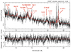 |
Fig. 2. RGS spectrum of A2667 overlaid with an isothermal model of gas in collisional equilibrium (red). Emission lines commonly detected in RGS spectra of CC clusters are labeled at the observed wavelengths. Dotted labels refer to lines from gas below 1 keV. Residuals are shown in the bottom panel. The dotted line in the upper panel represents the background spectrum. |
Not surprisingly, when we add a three-temperature bins (0.5−1.0, 1.0−2.0, 2.0−3.0 keV) CF model, we obtain only upper limits on the MDR, equal to Ṁ(0.5−1 keV) < 22 M⊙ yr−1 and Ṁ(1−2 keV) < 45 M⊙ yr−1. As expected, the 2−3 keV temperature bin is characterized by a large cooling rate 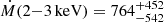 M⊙ yr−1. These results are statistically in agreement with the ones found in the EPIC spectra. However, we do not reproduce the 2σ detection of a CF in the 0.5−1 keV temperature bin.
Eventually, a more complex model with five temperature bins (0.1−0.5, 0.5−1.0, 1.0−2.0, 2.0−3.0, 3.0−7.0 keV) provide only upper limits on the amount of gas cooling within each temperature interval. We obtain Ṁ(0.1−0.5 keV) < 24 M⊙ yr−1, Ṁ(0.5−1.0 keV) < 22 M⊙ yr−1 and Ṁ(1.0−2.0 keV) < 44 M⊙ yr−1. Finally, when using a CF component with only two temperature bins (0.1−2.0, 2.0−7.0 keV), we obtain  M⊙ yr−1, and Ṁ(0.1−2.0 keV) < 11 M⊙ yr−1. We report the MDR of the CF component with five, three and two temperature bins in Table 4.
To discuss our results, including the analysis of EPIC data, we show the measured MDRs or their 1σ upper limits in Fig. 3. First, we note that all our results are in agreement with each other, except the measurement of a mass deposition rate of Ṁ = (46 ± 8) M⊙ yr−1 in the temperature interval 0.5−1 keV obtained with the combined analysis of all the EPIC spectra. This point is, in fact, about 3σ above the upper limits found by the analysis of RGS spectra. Nevertheless, it is clear that the maximum MDR allowed by an isobaric CF model is at least one order of magnitude lower than that measured in the 2−3 keV temperature bin, in agreement with results obtained in similar studies (Peterson et al. 2001; Sanders et al. 2010; Molendi et al. 2016). Given the overall agreement between the Ṁ values, we shall perform a joint EPIC and RGS fit in Sect. 7.
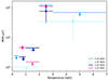 |
Fig. 3. RGS and EPIC cooling rates measurements and upper limits. In light blue, dark blue, and cyan, we show RGS values and upper limits on cooling rates obtained from a five-component, three-component and two-component CF model. In magenta, we show the EPIC measurements and upper limit of cooling rate obtained from the three-component CF model reported in Table 2 (see all stacked EPIC ObsID). |
6.3. Instrumental versus turbulent broadening
The spectral fits yield a maximum line width corresponding to a line broadening vmic(1D) = 710 ± 170 km s−1. This measurement, however, does not account for the fact that the broadening is expected to be dominated by the spatial extent of the source. The impact of this effect can be subtracted using the surface brightness modeled on the high-resolution Chandra images in the soft band [0.5−2 keV].
We produced Chandra surface brightness profiles to model the RGS line spatial broadening with the standard dispersion equation:
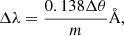 (2)
(2)
where Δλ is the wavelength broadening, Δθ is the source extent in arcseconds, and m is the spectral order (see the XMM-Newton Users Handbook4). The surface brightness was extracted using a region of 50″ width and a length of 10′ (which approximates an RGS extraction region; see Sect. 4.2), and using the CIAO task dmstat. The RGS instrumental line broadening measured through the Chandra surface brightness profile of A2667 cluster is shown in Fig. 4 (black line). It is well known that the spatial profiles extracted from the CCD images tend to overestimate the soft X-ray line broadening due to the contribution from the hotter continuum, which has a larger extent than the cooler gas producing such lines (Pinto et al. 2015). We therefore followed the approach outlined in Bambic et al. (2018) whereby only the core of the spatial profile was adopted. This can be estimated by fitting the broadening profile with either two or three multiple Gaussian lines depending on the cluster distance. Typically, for clusters beyond redshift 0.2, two Gaussian lines are sufficient (i.e., one for the core and the other for the ambient gas). The single Gaussian line (black line) obtained with Chandra data and the narrowest Gaussians (dotted green and red lines) of the multicomponent models fitting are also shown in Fig. 4, but renormalized for plotting purposes.
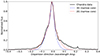 |
Fig. 4. RGS line spatial broadening computed through the Chandra surface brightness profile and Eq. (2) (black line). The lines show the narrowest Gaussian referring only to the cluster core obtained by fitting two different models with either two (dotted red line) or three (dotted blue line) Gaussian lines. |
Then, we used the lpro model in SPEX to take into account the instrumental broadening. The lpro model receives as input the spatial broadening measured with the Chandra surface brightness profile and convolves it with the baseline spectral model:
 (3)
(3)
The lpro component now accounts for the spatial broadening. As was mentioned before, we only accounted for the spatial extent of the CC in order to avoid over-subtraction of the spatial extent and under-estimate the upper limit on the turbulence. This was done by using the spatial broadening constrained by the narrower Gaussian that was used in the fit of the Chandra spatial profile. After fitting the RGS spectrum including the lpro component, the parameter vmic is now related only to the turbulent velocity. The large uncertainty associated with the subtraction of the source profile hampers us from obtaining a robust measurement. Indeed, we obtain a 90% upper limit of 561 km/s and 787 km/s for the velocity broadening in the case of two and three Gaussians, respectively. We note that the velocity broadening upper limits are higher than those found in the Phoenix cluster at high redshift, and of those measured in other clusters in the local Universe, such as Abell 1835 (Sanders et al. 2010), observed with comparable signal to noise. This could be due to the fact that in A2667 there are some ongoing processes boosting turbulence more than in typical CC clusters. This point will be discussed in detail in Sects. 8.2 and 8.4.
7. EPIC and RGS joint fit
To better characterize the system and place tighter constraints on cooling rates, we performed a joint fit of all available XMM-Newton spectra. We followed the strategy used for EPIC and RGS spectral fit separately in the previous sections. We described the ICM emission with an isothermal collisional equilibrium model, the AGN contribution with an absorbed power law, and we added a three-component CF model with temperature bins set to 0.5−1.0, 1.0−2.0, and 2.0−3.0 keV (see Sects. 5 and 6 for further details).
The best-fit values of the spectral parameters from the joint fit are shown in Table 5, while we report the best-fit model and data plots in Appendix C. We performed the joint fit in four steps: first, we combined RGS with the stacked spectrum of the MOS1 detectors, then MOS2, pn, and finally all the EPIC detectors together. We note that all the combinations are in agreement with each other, so we can rely on the fit obtained by stacking all the independent spectra extracted from our data as the result with the largest amount of information. We conclude that we find positive values within 1σ sigma confidence level for the MDR in the 0.5−1 keV temperature bin and only upper limits in the 1−2 keV temperature bin. These values and upper limits are in agreement with the analysis of the RGS spectrum within 1σ, and more in general with the values shown in Fig. 3.
XMM-Newton/RGS and EPIC joint best-fit isothermal cie model with a CF component with three temperature bins.
Finally, we note that the isobaric cooling may not be the only physical mechanism producing a MDR. Therefore, after having explored CF models in a limited temperature bin, we account also for the presence of nonisobaric modes by the wdem (Kaastra et al. 2004) model which describes the emission measure distribution of the ICM with a generic power law. The free parameters in this model are the emission measure value, maximum temperature, lower temperature cutoff, and iron abundance. The values found for the emission measure ( m−3), maximum temperature (Tmax = 6.30 ± 0.03 keV) and iron abundance (Fe/H = 0.62 ± 0.01) are in agreement with the values found with cie model, but with a much higher C-stat value (C-stat = 1927/1100). Moreover, we are not able to constrain the value of the low-temperature cutoff (Tcut < 0.13 keV). We conclude that the gas distribution in this cluster does not follow a power law, as has also been found by a similar analysis in the literature (see Frank et al. 2013).
8. Discussion
8.1. Cooling rates
In this work, we study the galaxy cluster A2667 in order to understand how much gas is cooling below 2 keV. Considering the fitting procedure of the RGS and EPIC data, we can only put an upper limit on the values of cooling rate in the temperature ranges 0.5−1 keV and 1−2 keV. In particular, in the range 0.5−1 keV, we have a 1σ upper limit of ∼36 M⊙ yr−1, while in the range of 1−2 keV we have an upper limit of ∼60 M⊙ yr−1. On the one hand, in the RGS spectrum we only find evidence of the OVIII line directly associated to ∼1 keV ICM. On the other hand, we do not significantly detect either FeXXI-FeXXII and FeXVII forbidden, intercombination, and resonant emission lines, or OVII, which are the best tracers for ≲1 keV gas (see e.g., Sanders et al. 2010). Probably, the OVII lines are hidden within the noise and the high instrumental background around 35 Å. However, the absence of FeXXI-FeXXII should clearly indicate that the amount of gas cooling below 1 keV is minimal. Also, since the difference measured in the cooling rates between 1−2 keV and 2−3 keV is larger than 1000 M⊙ yr−1, it looks like the gas is not able to cool below 2 keV because of reheating by some feedback mechanism. As is supported by high-resolution hydrodynamical simulations, the sudden drop of the emission measure below 2 keV is likely due to a combination of the direct AGN heating and turbulent mixing, which induce nonisobaric modes into the (quenched) CF (Gaspari 2015).
These results, combined with the presence of an AGN with a low nuclear power (∼3 × 1043 erg/s, Yang et al. 2018), could imply that we are either in the presence of a minimal MDR in the aftermath of a cooling event powering off, or the beginning of a cooling episode that has just awakened the AGN. In this second case, the BCG may evolve within a few tens of millions of years into a Phoenix-like phase, with a rise in the value of the MDR promptly counterbalanced by strong feedback. A relevant quantity in this respect would be an estimate of average AGN feedback power in the last tens of Myr, for example from ICM cavities. Moreover, it would be important to assess the dynamical state of the clusters to evaluate the presence of induced sloshing in the ICM or to identify a recent minor merger onto the BCG. We shall discuss some of these aspects in the next subsections.
8.2. Cooling-heating equilibrium
In our attempt to place constraints on turbulence and estimate whether the energy stored in turbulent motions is high enough to balance radiative cooling, we obtained a total broadening of the emission lines in the RGS spectrum of 710 ± 170 km s−1. As is described in Sect. 6.3, after modeling the spatial broadening due to the spatial extent of the source with two Gaussian curves, we obtain 90% upper limits on the turbulent broadening, equal to 561 km s−1, or even higher for more accurate modelization of the source profile. This limit is well above the turbulence level required to propagate the heat throughout the Phoenix cluster at z ∼ 0.6 from the central AGN up to 250 kpc (Pinto et al. 2018). This suggests that in A2667 the ICM may be characterized by a high level of turbulence, consistent with a post-feedback scenario.
To achieve a rough estimate of the turbulent velocity in the ICM of A2667, we can adopt the simplified, model-dependent approach proposed by Sanders & Fabian (2013). This consists of computing the intrinsic broadening as the difference between the square of the total width obtained from the RGS spectral fit (710 km/s) and the instrumental broadening estimated simply by the full width half maximum of the Gaussian describing the core spatial extent. The broadening in units of velocity is obtained from the relation
 (4)
(4)
where σ = 0.04 is the Gaussian width obtained with the Python routine leastsq, λ is the RGS band center at ∼19 Å (position of O VIII emission line peak), and c is the speed of light. We obtain an intrinsic broadening of 320 ± 200 km s−1. However, this result is an optimistic estimate of the error. If we consider all the uncertainties in our approach, this result can be considered as a 1σ upper limit. We have to rely on future bolometer measurements (e.g., XRISM; see Sect. 9) to provide greater precision and allow us to confirm or refine this estimate.
As has been probed by high-resolution hydrodynamical simulations, such levels of turbulent velocities (and related enstrophy) are enough to enhance local thermal instability and trigger a condensation rain of warm filaments or clouds, which is expected to boost the SMBH accretion rates via CCA during the next self-regulation cycle (Gaspari et al. 2020). Indeed, the SMBH mass of A2667 is 2 × 10¹⁰ M⊙ (Phipps et al. 2019), which can be achieved only through recurrent flickering cycles of CCA feeding, unlike in hot-mode (Bondi/ADAF) scenarios (see the Discussion section in Gaspari et al. 2019). Quantitatively, we computed a key CCA diagnostics; that is, the condensation ratio, C ≡ tcool/teddy, within the putative bubble region (L ∼ 25 kpc), which is also comparable to typical condensation core sizes (Wang et al. 2023). We find a C ratio of 0.4, which is consistent with an ensuing or resuming CCA rain, as it crosses the C ∼ 1 threshold (Gaspari et al. 2018).
8.3. Comparison with Abell 1835
To have a better grasp on the level of turbulence in A2667, we confronted the intrinsic broadening value obtained for A2667 with the one obtained from Abell 1835 (hereafter A1835) Chandra surface brightness profile. We used this cluster because is placed at a redshift close to that of A2667 – z = 0.2523 – and shows a CC at the center. In addition, considering the total luminosity of both clusters, their temperature and the XMM-Newton exposure time, the X-ray signal from A1835 is about 4.5 times larger than A2667. A1835 is the most luminous cluster in the ROSAT Bright Cluster Sample (Ebeling et al. 1998), with an inferred isobaric CF cooling rate of ∼1000 M⊙ yr−1 (Allen et al. 1996). The SFR in the central galaxy derived from optical spectroscopic is 40−70 M⊙ yr−1 (Crawford et al. 1999). The infrared luminosity of the object is ∼7 × 10¹¹ L⊙ (Egami et al. 2006), suggesting an even higher SFR up to ∼125 M⊙ yr−1. In addition a total mass of ∼5 × 10¹⁰ M⊙ of molecular gas has been measured within 10 kpc from the BCG center (McNamara et al. 2014). Despite the evidence for star formation, cool gas and the high X-ray luminosity (LX[0.1 − 2.4 keV] ∼ 3.9 × 1045 erg s−1; Ebeling et al. 1998), little X-ray emitting gas was seen in this cluster below 1−2 keV when it was observed using the XMM-Newton RGS instruments (Peterson et al. 2001). More quantitatively, fewer than 200 M⊙ yr−1 cools below 2.7 keV (90% confidence) and far below 100 M⊙ yr−1 at lower temperatures (Liu et al. 2019b). Therefore, it has been proposed that AGN feedback, estimated to have an average of 1.4 × 1045 erg/s in the last few tens of millions of years, prevents most of the X-ray gas from cooling (McNamara et al. 2006).
Using XMM-RGS data, Sanders et al. (2010) calculate the line-of-sight, nonthermal, total broadening of A1835, finding a 90% upper limit value of 222 km/s. This value is lower than our measurement of the total broadening in A2667 equal to 710 ± 160 km s−1 (see Sect. 6.1). We attempt to estimate the turbulent velocity component in A1835 after computing the source spatial broadening in the simplified method described in Sect. 8.2.
We used 30 ks of archival ACIS data from the Chandra archive to derive the surface brightness profile of A1835. We reduced the data following the procedure described in Sect. 3. We obtained the line spatial broadening fitting the data with three Gaussian lines (see red and orange lines in Fig. 5), as described in Sect. 6.3. Then, we applied the relation (4), where σ = 0.01 was obtained by the Python routine leastsq. We obtained an upper limit on the velocity broadening of 170 km/s (90% confidence level) that can be ascribed to turbulent motions.
 |
Fig. 5. Line spatial broadening computed through the Chandra surface brightness profile and Eq. (2) for A2667 (blue line) and Abell 1835 (red line). The dash-dotted turquoise line and the dashed orange line show the narrowest Gaussian obtained by fitting three Gaussian lines for A2667 and Abell 1835, respectively. |
The striking difference between the line broadening of A2667 with respect to A1835 can be seen in Fig. 5. We note that the spatial broadening in A1835 is ∼50% lower than the spatial broadening in A2667 and this reflects on the turbulent velocity line broadening which is at least double in A2667 with respect to A1835. It has been argued that the central AGN in A1835 is not inducing large amounts of turbulence in the ICM in the cluster core (Sanders et al. 2010). Given our results, we suggest that in A2667 turbulent velocity may be boosted by physical processes such as AGN mechanical feedback, sloshing, and/or minor mergers, or, more likely, a combination of them. We tentatively quantify this effect to be a factor of 2 with respect to A1835 and other similar CC clusters (see clusters in Sanders & Fabian 2013 sample). To summarize, it will be extremely interesting to obtain tighter constraints on the turbulence in A2667 with X-ray bolometers, as is discussed in Sect. 9.
8.4. Possible role of minor mergers, sloshing, and AGN feedback in heating processes
In previous sections, we mentioned minor mergers, sloshing and AGN feedback as possible mechanisms for boosting turbulent velocity and reheating the ICM preventing or strongly reducing cooling in the gas below 2 keV in A2667. Considering the resolution of current data, we cannot rule out one mechanism or identify the dominance of another. Here, we review different hints on the role of these mechanisms based on the available literature. Indeed, according to previous studies, especially Giacintucci et al. (2019) and Iani et al. (2019), there is convincing evidence of the presence of all these mechanisms.
Iani et al. (2019) find the presence of a complex system of substructures in the optical surface brightness extending all around the BCG at the center of A2667 using HST and MUSE data, characterized by a strong blue optical color suggesting a young stellar population. They propose two scenarios to explain the presence of filaments and clumps, one associated with the AGN feedback and the other associated with the presence of a companion galaxy falling onto the BCG. Particularly, for the second scenario the clumps appear to lie on the BCG galactic plane, as it would happen with an accreting satellite galaxy that loses its angular momentum and starts inspiralling toward the BCG center. At the opposite extremity of the galaxy with respect to the clumps in the HST images, diffuse blue emission is present, likely due to the gas left behind by the satellite galaxy from a previous orbit. The presence of a satellite galaxy could favor the presence of minor mergers which influence the heating and cooling of the gas around the BCG and in the cluster. Instead, they tend to exclude the first scenario on the AGN feedback because even though the clumps are observed on a physical scale of ∼10−20 kpc from the galaxy nucleus, Chandra X-ray data and JVLA-ALMA radio data do not show a clear presence of jets or inflated bubbles on a large scale. However, if we improve the contrast of Chandra image using the unsharp mask procedure in CIAO, we find clear asymmetric features at a distance of roughly 90 kpc and 50 kpc from the center of the BCG, as is shown in Fig. 6. The shape of the features is reminiscent of a cold front, however, the surface brightness depression regions are quite extended, and we cannot exclude the presence of cavities. Given the very shallow archival exposure, and the high flux of A2667, a moderately deeper Chandra observation would significantly improve the characterization of the surface brightness edges or cavities detected in current data. This would bring another piece of information that is relevant for identifying the main source of heating in the core of A2667.
 |
Fig. 6. Chandra 0.3−10 keV unsharp mask image of A2667. The white arrows are adapted from Giacintucci et al. (2019) and represent the two surface brightness edges found, which may be cold fronts or bubble-like features. |
Focusing on the radio band, Giacintucci et al. (2019) find the presence of a minihalo using GMRT-VLA radio data which covers an area of ∼70 kpc in radius. They also discuss the two surface brightness features in the X-ray image (see white arrows in Fig. 6) and interpret them as cold fronts. Indeed, the radio minihalo seems to be contained within the sloshing region defined by the X-ray fronts. These results stress the presence of sloshing in the ICM of A2667. To conclude, the combination of high-resolution X-ray spectra and high-resolution X-ray images is required to comprehend the dynamical and thermodynamical state of the ICM in the core of A2667.
9. Future perspectives
Current X-ray instruments on board XMM-Newton and Chandra only allow us to obtain approximate turbulent velocity measurements and also have limitations due to source extent and associated broadening. The most accurate measurement of line broadening and, therefore, constraint on turbulence in the ICM, was obtained by the Hitomi satellite (Takahashi et al. 2010) during its deep (230 ks) observation of the Perseus cluster of galaxies (Hitomi Collaboration 2016), but this satellite was lost immediately afterward in 2016. However, a new X-Ray Imaging and Spectroscopy Mission (XRISM; Guainazzi & Tashiro 2019) was launched in 2023.
We therefore performed a simulation of A2667 as it will be seen by XRISM using a gate-valve-closed (GVC) Resolve response matrix with a 5 eV spectral resolution using SPEX command simulate. We considered the XMM/EPIC+XMM/RGS best fit model (cie model; see Sects. 5 and 6) and assumed an exposure time of 250 ks with GVC, similar to that of the Perseus cluster.
We assume a line broadening due to turbulent velocity of 320 km s−1 as in our simple estimate (see Sect. 8.2). The simulated spectrum is shown in Fig. 7. We can see that we are able to resolve the Fe XXV multiplet emission lines in the energy range of 5−6 keV. We can place tight constraints on turbulent velocity corresponding to a statistical uncertainty of just ∼30 km s−1 for a 250 ks XRISM observation, obtaining much stronger constraints compared to those in this work.
 |
Fig. 7. Simulation of an A2667 observation with XRISM/Resolve accounting for the GVC. The black dots are data points and the red line is the best-fit isothermal model. The plot is zoomed on the region of the FeXXV-XXVI lines in the observer frame. |
Another instrument that will bring a drastic improvement is the X-ray Integral Field Unit (X-IFU) on board the Advanced Telescope for High Energy Astrophysics (ATHENA; Nandra et al. 2013) that has been rescoped to the novel mission design NewAthena and is expected to be operating in the late 2030s. This satellite will provide a spatial resolution down to around 9 arcsec (half energy width), a spectral resolution of ∼2.5 eV, and an effective area of more than an order of magnitude larger than any previous grating or microcalorimeter, implying a significant improvement in our capabilities to investigate the X-ray spectra of galaxy clusters. We performed a NewAthena simulation of A2667 using a gate-valve-open (GVO) X-IFU response matrix (as of July 2024). We considered the same template model used for XRISM simulation with the addition of a CF model with three temperature bins, but with an exposure time of 300 ks, higher than the 250 ks used for the XRISM simulation.
The X-IFU 300 ks observation of A2667 will provide a spectacular spectrum of high quality (see Fig. 8) and will allow us to measure velocity broadening with statistical uncertainties of ∼6 km s−1, much tighter constraints on turbulence compared to the XRISM observations. This also happens for cooling rates measurements, for which we obtain statistical uncertainties of ∼10 − 20% (0.5−1.0 keV) on an MDR of 10 M⊙ yr−1. For the temperature bin 1.0−2.0 keV, on the other hand, it is still difficult to get this level of uncertainty. Indeed, to obtain statistical uncertainties of ∼10 − 20% on the MDR in the range 1.0−2.0 keV we need observations of 3 Ms.
 |
Fig. 8. Simulation of an A2667 observation with ATHENA/X-IFU. The black dots are data points and the red line is the best-fit isothermal model + isobaric CF model in three temperature bins. |
With NewAthena, we are also able to put constraints on the temperature truncation value of the cooling gas. In a simulation with an input isobaric CF with a minimum temperature of 0.7 keV, and Ṁ = 100 M⊙ yr−1, we are able to recover the truncation temperature with a 1σ error of 4%, and the MDR with a 1σ error of 8%. We conclude that with XRISM and NewAthena we shall be able to investigate the cooling and heating mechanisms in A2667, and finally constrain the different scenarios outlined in this work.
10. Conclusions
In this paper, we have studied the thermal X-ray emission from the ICM in the CC cluster A2667 at redshift z = 0.233, focusing on the core region included within a radius of ∼115 kpc. We performed a detailed analysis of the deep XMM-Newton observations of A2667, along with archival Chandra data.
From the X-ray spectral analysis of XMM/EPIC and RGS data, we conclude that we are able to put only upper limits on the MDR in the ICM below 2 keV. In particular, we find Ṁ < 36 M⊙ yr−1 (0.5−1 keV) and Ṁ < 58 M⊙ yr−1 (1−2 keV). We measure a cooling rate in the temperature interval 2−3 keV equal to  M⊙ yr−1. These results envisage a scenario in which the maximum amount of gas cooling below 2 keV is below ∼4−5% of gas cooling in the range 2−3 keV. Thus, we can say that A2667 is not different from other low-redshift CC clusters.
Interestingly, from XMM/RGS spectral fitting, using a cie model, we find a maximum line broadening corresponding to 710 ± 170 km s−1, which includes both spatial and turbulent broadening, along with instrumental broadening. We make a simple estimate of the intrinsic, turbulent velocity of ∼320 ± 200 km s−1, a value that is at least twice the one estimated in the local cluster A1835. These limits are well above the turbulence required to propagate the heat throughout the Phoenix cluster at z ∼ 0.6 from the central AGN up to 250 kpc. This result could be considered as a hint of the fact that there are some processes ongoing in A2667 that boost turbulence and quench cooling, such as sloshing, minor mergers, and/or AGN feedback. At the same time, it is important to note that turbulence stimulates local thermal instability, and hence vitally promotes the next generation of CCA rain, as is shown by the computed low C ratio of 0.4 in the core of A2667. Imaging analysis with high-resolution Chandra data provide clear surface brightness depression that can be interpreted as the signatures of a cold front or the presence of ICM cavities.
Current XRISM and future NewAthena missions will improve the accuracy in measuring crucial parameters in X-ray spectra of clusters of galaxies. Particularly, it is already possible to bring the uncertainty on the turbulent velocity in A2667 down to ∼10% (∼30 km s−1 in our case) with a 250 ks XRISM observation. With NewAthena it will be possible to further reduce this uncertainty to ∼3%. Unfortunately, a robust assessment of the actual MDR at the level of ∼10 M⊙ yr−1, as we expect in A2667, will be possible only with an X-ray bolometer with sensitivity below 2 keV, such as the X-IFU on board NewAthena. This implies that the characterization and quantification of the CFs hosted by CC clusters directly measured from X-ray is at present severely limited by current facilities.
See “Users Guide to the XMM-Newton Science Analysis System”, Issue 18.0, 2023 (ESA: XMM-Newton SOC).
Acknowledgments
We thank the anonymous referee for the detailed comments and positive criticism that helped us improve the quality of this manuscript. M.L. and P.T. acknowledge the program INAF Fundamental Astrophysics 2023 “The origin of cool cores and the evolution of BCGs in galaxy clusters”. M.L. further acknowledges the support from the ESO Scientific Visitor Programme. M.L. also acknowledges support from the PRIN MIUR 2020 GRAAL 2020SKSTHZ. C.P. is supported by PRIN MUR 2022 SEAWIND 2022Y2T94C funded by European Union – Next Generation EU. M.G. acknowledges support from the ERC Consolidator Grant BlackHoleWeather (101086804).
References
- Allen, S. W., Fabian, A. C., Edge, A. C., et al. 1996, MNRAS, 283, 263 [NASA ADS] [CrossRef] [Google Scholar]
- Bambic, C. J., Pinto, C., Fabian, A. C., Sanders, J., & Reynolds, C. S. 2018, MNRAS, 478, L44 [NASA ADS] [CrossRef] [Google Scholar]
- Cavagnolo, K. W., Donahue, M., Voit, G. M., & Sun, M. 2009, ApJS, 182, 12 [Google Scholar]
- Cavaliere, A., & Fusco-Femiano, R. 1978, A&A, 70, 677 [NASA ADS] [Google Scholar]
- Covone, G., Kneib, J. P., Soucail, G., et al. 2006a, A&A, 456, 409 [NASA ADS] [CrossRef] [EDP Sciences] [Google Scholar]
- Covone, G., Adami, C., Durret, F., et al. 2006b, A&A, 460, 381 [NASA ADS] [CrossRef] [EDP Sciences] [Google Scholar]
- Crawford, C. S., Allen, S. W., Ebeling, H., Edge, A. C., & Fabian, A. C. 1999, MNRAS, 306, 857 [CrossRef] [Google Scholar]
- de Plaa, J., Kaastra, J. S., Werner, N., et al. 2017, A&A, 607, A98 [NASA ADS] [CrossRef] [EDP Sciences] [Google Scholar]
- Donahue, M., & Voit, G. M. 2004, in Clusters of Galaxies: Probes of Cosmological Structure and Galaxy Evolution, eds. J. S. Mulchaey, A. Dressler, & A. Oemler, 143 [Google Scholar]
- Ebeling, H., Edge, A. C., Bohringer, H., et al. 1998, MNRAS, 301, 881 [Google Scholar]
- Egami, E., Misselt, K. A., Rieke, G. H., et al. 2006, ApJ, 647, 922 [NASA ADS] [CrossRef] [Google Scholar]
- Ettori, S., Fabian, A. C., Allen, S. W., & Johnstone, R. M. 2002, MNRAS, 331, 635 [Google Scholar]
- Fabian, A. C. 1994, ARA&A, 32, 277 [Google Scholar]
- Fabian, A. C. 2012, ARA&A, 50, 455 [Google Scholar]
- Fabian, A. C., & Nulsen, P. E. J. 1977, MNRAS, 180, 479 [NASA ADS] [CrossRef] [Google Scholar]
- Fabian, A. C., Sanders, J. S., Allen, S. W., et al. 2003, MNRAS, 344, L43 [NASA ADS] [CrossRef] [Google Scholar]
- Fabian, A. C., Sanders, J. S., Taylor, G. B., et al. 2006, MNRAS, 366, 417 [NASA ADS] [CrossRef] [Google Scholar]
- Fabian, A. C., Sanders, J. S., Allen, S. W., et al. 2011, MNRAS, 418, 2154 [Google Scholar]
- Fabian, A. C., Ferland, G. J., Sanders, J. S., et al. 2022, MNRAS, 515, 3336 [NASA ADS] [CrossRef] [Google Scholar]
- Frank, K. A., Peterson, J. R., Andersson, K., Fabian, A. C., & Sanders, J. S. 2013, ApJ, 764, 46 [Google Scholar]
- Gaspari, M. 2015, MNRAS, 451, L60 [NASA ADS] [CrossRef] [Google Scholar]
- Gaspari, M., Ruszkowski, M., & Sharma, P. 2012, ApJ, 746, 94 [Google Scholar]
- Gaspari, M., McDonald, M., Hamer, S. L., et al. 2018, ApJ, 854, 167 [Google Scholar]
- Gaspari, M., Eckert, D., Ettori, S., et al. 2019, ApJ, 884, 169 [NASA ADS] [CrossRef] [Google Scholar]
- Gaspari, M., Tombesi, F., & Cappi, M. 2020, Nat. Astron., 4, 10 [Google Scholar]
- Gastaldello, F., Simionescu, A., Mernier, F., et al. 2021, Universe, 7, 208 [NASA ADS] [CrossRef] [Google Scholar]
- Giacintucci, S., Markevitch, M., Cassano, R., et al. 2017, ApJ, 841, 71 [Google Scholar]
- Giacintucci, S., Markevitch, M., Cassano, R., et al. 2019, ApJ, 880, 70 [Google Scholar]
- Gilmour, R., Best, P., & Almaini, O. 2009, MNRAS, 392, 1509 [NASA ADS] [CrossRef] [Google Scholar]
- Guainazzi, M., & Tashiro, M. 2019, Proceedings of the IAU Symposium No. IAUS342 [Google Scholar]
- HI4PI Collaboration (Ben Bekhti, N., et al.) 2016, A&A, 594, A116 [NASA ADS] [CrossRef] [EDP Sciences] [Google Scholar]
- Hitomi Collaboration (Aharonian, F., et al.) 2016, Nature, 535, 117 [Google Scholar]
- Hudson, D. S., Mittal, R., Reiprich, T. H., et al. 2010, A&A, 513, A37 [NASA ADS] [CrossRef] [EDP Sciences] [Google Scholar]
- Iani, E., Rodighiero, G., Fritz, J., et al. 2019, MNRAS, 487, 5593 [NASA ADS] [CrossRef] [Google Scholar]
- Kaastra, J. S., Mewe, R., & Nieuwenhuijzen, H. 1996, UV and X-ray Spectroscopy of Astrophysical and Laboratory Plasmas, 411 [Google Scholar]
- Kaastra, J. S., Ferrigno, C., Tamura, T., et al. 2001, A&A, 365, L99 [NASA ADS] [CrossRef] [EDP Sciences] [Google Scholar]
- Kaastra, J. S., Tamura, T., Peterson, J. R., et al. 2004, A&A, 413, 415 [NASA ADS] [CrossRef] [EDP Sciences] [Google Scholar]
- Kadam, S. K., Sonkamble, S. S., Pawar, P. K., & Patil, M. K. 2019, MNRAS, 484, 4113 [NASA ADS] [CrossRef] [Google Scholar]
- Kale, R., Venturi, T., Cassano, R., et al. 2015, A&A, 581, A23 [NASA ADS] [CrossRef] [EDP Sciences] [Google Scholar]
- Knowles, K., Cotton, W. D., Rudnick, L., et al. 2022, A&A, 657, A56 [NASA ADS] [CrossRef] [EDP Sciences] [Google Scholar]
- Liu, A., Zhai, M., & Tozzi, P. 2019a, MNRAS, 485, 1651 [NASA ADS] [CrossRef] [Google Scholar]
- Liu, H., Pinto, C., Fabian, A. C., Russell, H. R., & Sanders, J. S. 2019b, MNRAS, 485, 1757 [NASA ADS] [CrossRef] [Google Scholar]
- Liu, A., Tozzi, P., Ettori, S., et al. 2020, A&A, 637, A58 [NASA ADS] [CrossRef] [EDP Sciences] [Google Scholar]
- Liu, W., Sun, M., Voit, G. M., et al. 2024, MNRAS, 531, 2063 [NASA ADS] [CrossRef] [Google Scholar]
- Lodders, K., & Palme, H. 2009, Meteor. Planet. Sci. Suppl., 72, 5154 [Google Scholar]
- Maccagni, F. M., Serra, P., Murgia, M., et al. 2021, in Galaxy Evolution and Feedback across Different Environments, eds. T. Storchi Bergmann, W. Forman, R. Overzier, & R. Riffel, 359, 141 [NASA ADS] [Google Scholar]
- Mann, A. W., & Ebeling, H. 2012, MNRAS, 420, 2120 [NASA ADS] [CrossRef] [Google Scholar]
- Mantz, A. B., Allen, S. W., Morris, R. G., & Schmidt, R. W. 2016, MNRAS, 456, 4020 [NASA ADS] [CrossRef] [Google Scholar]
- McDonald, M., Bayliss, M., Benson, B. A., et al. 2012, Nature, 488, 349 [Google Scholar]
- McDonald, M., McNamara, B. R., van Weeren, R. J., et al. 2015, ApJ, 811, 111 [Google Scholar]
- McDonald, M., Gaspari, M., McNamara, B. R., & Tremblay, G. R. 2018, ApJ, 858, 45 [Google Scholar]
- McDonald, M., McNamara, B. R., Voit, G. M., et al. 2019, ApJ, 885, 63 [NASA ADS] [CrossRef] [Google Scholar]
- McKinley, B., Tingay, S. J., Gaspari, M., et al. 2022, Nat. Astron., 6, 109 [Google Scholar]
- McNamara, B. R., & Nulsen, P. E. J. 2007, ARA&A, 45, 117 [NASA ADS] [CrossRef] [Google Scholar]
- McNamara, B. R., Wise, M., Nulsen, P. E. J., et al. 2000, ApJ, 534, L135 [NASA ADS] [CrossRef] [Google Scholar]
- McNamara, B. R., Nulsen, P. E. J., Wise, M. W., et al. 2005, Nature, 433, 45 [NASA ADS] [CrossRef] [PubMed] [Google Scholar]
- McNamara, B. R., Rafferty, D. A., Bîrzan, L., et al. 2006, ApJ, 648, 164 [NASA ADS] [CrossRef] [Google Scholar]
- McNamara, B. R., Russell, H. R., Nulsen, P. E. J., et al. 2014, ArXiv e-prints [arXiv:1403.4249] [Google Scholar]
- Merloni, A., Heinz, S., & di Matteo, T. 2003, MNRAS, 345, 1057 [Google Scholar]
- Mernier, F., de Plaa, J., Kaastra, J. S., et al. 2017, A&A, 603, A80 [NASA ADS] [CrossRef] [EDP Sciences] [Google Scholar]
- Mittal, R., McDonald, M., Whelan, J. T., & Bruzual, G. 2017, MNRAS, 465, 3143 [NASA ADS] [CrossRef] [Google Scholar]
- Molendi, S., & Pizzolato, F. 2001, ApJ, 560, 194 [NASA ADS] [CrossRef] [Google Scholar]
- Molendi, S., Tozzi, P., Gaspari, M., et al. 2016, A&A, 595, A123 [NASA ADS] [CrossRef] [EDP Sciences] [Google Scholar]
- Nandra, K., Barret, D., Barcons, X., et al. 2013, ArXiv e-prints [arXiv:1306.2307] [Google Scholar]
- North, E. V., Davis, T. A., Bureau, M., et al. 2021, MNRAS, 503, 5179 [NASA ADS] [CrossRef] [Google Scholar]
- Olivares, V., Salomé, P., Hamer, S. L., et al. 2022, A&A, 666, A94 [NASA ADS] [CrossRef] [EDP Sciences] [Google Scholar]
- Pasini, T., Gitti, M., Brighenti, F., et al. 2021, ApJ, 911, 66 [NASA ADS] [CrossRef] [Google Scholar]
- Peterson, J. R., & Fabian, A. C. 2006, Phys. Rep., 427, 1 [Google Scholar]
- Peterson, J. R., Paerels, F. B. S., Kaastra, J. S., et al. 2001, A&A, 365, L104 [NASA ADS] [CrossRef] [EDP Sciences] [Google Scholar]
- Phipps, F., Bogdán, Á., Lovisari, L., et al. 2019, ApJ, 875, 141 [NASA ADS] [CrossRef] [Google Scholar]
- Pinto, C., Sanders, J. S., Werner, N., et al. 2015, A&A, 575, A38 [NASA ADS] [CrossRef] [EDP Sciences] [Google Scholar]
- Pinto, C., Bambic, C. J., Sanders, J. S., et al. 2018, MNRAS, 480, 4113 [NASA ADS] [CrossRef] [Google Scholar]
- Planck Collaboration VI. 2020, A&A, 641, A6 [NASA ADS] [CrossRef] [EDP Sciences] [Google Scholar]
- Rawle, T. D., Edge, A. C., Egami, E., et al. 2012, ApJ, 747, 29 [NASA ADS] [CrossRef] [Google Scholar]
- Rizza, E., Burns, J. O., Ledlow, M. J., et al. 1998, MNRAS, 301, 328 [NASA ADS] [CrossRef] [Google Scholar]
- Russell, H. R., Fabian, A. C., McNamara, B. R., & Broderick, A. E. 2015, MNRAS, 451, 588 [NASA ADS] [CrossRef] [Google Scholar]
- Sanders, J. S., & Fabian, A. C. 2007, MNRAS, 381, 1381 [Google Scholar]
- Sanders, J. S., & Fabian, A. C. 2013, MNRAS, 429, 2727 [NASA ADS] [CrossRef] [Google Scholar]
- Sanders, J. S., Fabian, A. C., Smith, R. K., & Peterson, J. R. 2010, MNRAS, 402, L11 [NASA ADS] [CrossRef] [Google Scholar]
- Sanders, J. S., Fabian, A. C., Sun, M., et al. 2014, MNRAS, 439, 1182 [NASA ADS] [CrossRef] [Google Scholar]
- Santos, J. S., Tozzi, P., Rosati, P., & Böhringer, H. 2010, A&A, 521, A64 [NASA ADS] [CrossRef] [EDP Sciences] [Google Scholar]
- Sonkamble, S. S., Kadam, S. K., Paul, S., et al. 2024, JApA, 45, 23 [Google Scholar]
- Takahashi, T., Mitsuda, K., Kelley, R., et al. 2010, SPIE Conf. Ser., 7732, 77320Z [NASA ADS] [Google Scholar]
- Tamura, T., Kaastra, J. S., Peterson, J. R., et al. 2001, A&A, 365, L87 [NASA ADS] [CrossRef] [EDP Sciences] [Google Scholar]
- Timmerman, R., van Weeren, R. J., Botteon, A., et al. 2022, A&A, 668, A65 [NASA ADS] [CrossRef] [EDP Sciences] [Google Scholar]
- Tozzi, P., Gastaldello, F., Molendi, S., et al. 2015, A&A, 580, A6 [NASA ADS] [CrossRef] [EDP Sciences] [Google Scholar]
- Vantyghem, A. N., McNamara, B. R., Russell, H. R., et al. 2014, MNRAS, 442, 3192 [Google Scholar]
- van Weeren, R. J., Intema, H. T., Lal, D. V., et al. 2014, ApJ, 786, L17 [NASA ADS] [CrossRef] [Google Scholar]
- Wang, L., Tozzi, P., Yu, H., Gaspari, M., & Ettori, S. 2023, A&A, 674, A102 [NASA ADS] [CrossRef] [EDP Sciences] [Google Scholar]
- Werner, N., Allen, S. W., & Simionescu, A. 2012, MNRAS, 425, 2731 [NASA ADS] [CrossRef] [Google Scholar]
- Wittor, D., & Gaspari, M. 2020, MNRAS, 498, 4983 [NASA ADS] [CrossRef] [Google Scholar]
- Wittor, D., & Gaspari, M. 2023, MNRAS, 521, L79 [NASA ADS] [CrossRef] [Google Scholar]
- Xu, H., Kahn, S. M., Peterson, J. R., et al. 2002, ApJ, 579, 600 [NASA ADS] [CrossRef] [Google Scholar]
- Yang, L., Tozzi, P., Yu, H., et al. 2018, ApJ, 859, 65 [NASA ADS] [CrossRef] [Google Scholar]
- Zhang, C., Xu, H., Zhu, Z., et al. 2016, ApJ, 823, 116 [NASA ADS] [CrossRef] [Google Scholar]
Appendix A: Impact of active galactic nuclei variability on the fitting procedure
In this work, we modeled the AGN component in the fitting process using a power law with the intrinsic absorption, NH, photon index, Γ, and luminosity, LX, fixed to the best-fit values obtained in Yang et al. (2018). In addition, we did not account for AGN variability. However, the values for NH and luminosity have rather large statistical uncertainties:  and
and ![Mathematical equation: $ \mathrm{log(L_{X})[erg/s]=43.4^{+0.2}_{-0.4}} $](/articles/aa/full_html/2025/02/aa52396-24/aa52396-24-eq40.gif) . In this appendix, we have performed additional tests and seen if there are some variations in the parameters relevant to our science goals associated with uncertainties in the AGN modelization. We thus allowed the intrinsic absorption and luminosity to vary within their respective 1σ error bounds, keeping Γ fixed to 1.8.
. In this appendix, we have performed additional tests and seen if there are some variations in the parameters relevant to our science goals associated with uncertainties in the AGN modelization. We thus allowed the intrinsic absorption and luminosity to vary within their respective 1σ error bounds, keeping Γ fixed to 1.8.
The results of these tests show no substantial differences in the fit parameters, with variations limited to within 5% in most of the best-fit values. We further extended the analysis by considering 2σ and 3σ deviations. Also, in this case, the variations are limited to 5% at most. These findings suggest that the variability of the AGN parameters within the observed error bounds does not affect the conclusions of this paper.
Appendix B: EPIC spectra
In this section we present the best-fit model plots of the stacked EPIC MOS1, MOS2, and pn spectra, along with the joint fit of all datasets. The spectra and corresponding best-fit models are shown in Fig. B.1, where we also display each model component: the power-law and cie components representing the ICM and AGN, as well as the three temperature bins of the CF component. The detailed fitting results are provided in Table 2.
The plots reveal some residuals below 2 keV, particularly in the spectra from ObsID 0900280101 and 0900280201, which are the newly added observations. In contrast, these residuals are not evident in the spectrum from the older ObsID 0148990101. The discrepancies observed in the new data may be attributed to the higher signal-to-noise ratio of these new deeper observations compared to the older dataset. This increased sensitivity can amplify the impact of systematic uncertainties. Indeed, there are known calibration uncertainties of 5-10%5 in EPIC/MOS and EPIC/pn data, which may contribute to the observed residuals. To address this issue, we also calculate the residuals in percentages below 2 keV. We found that they are consistent with 10%.
It is also worth noting that the current model may not fully capture the features of the new observations, particularly the emission lines below 1 keV. This suggests that further refinement of the model, for example with additional local fitting procedures (as in Mernier et al. 2017) or additional components, might be necessary to better characterize these data.
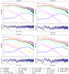 |
Fig. B.1. Spectral fit of MOS1+MOS2 (light blue and green points) and pn (purple points) data for ObsID 0148990101 (upper left panel), 0900280101 (upper right panel), 0900280201 (lower left panel) and all stacked spectra (lower right panel). Residuals are shown in the bottom panel. The model used for fitting is the combination of cie and the isobaric CF split into three temperature intervals. The model components are represented with different colors and line styles in the plots. Orange lines represent the cie component, and blue lines represent the power law component describing the ICM and AGN, respectively. Magenta, gold, and light green lines represent the three temperature bins (0.5-1, 1-2, and 2-3 keV) components. |
Appendix C: EPIC and RGS joint fit spectra
In this section we present the best-fit model plots of the RGS and EPIC joint fit. The spectra and corresponding best-fit models are shown in Fig. C.1, where we also display each model component: the power-law and cie components representing the ICM and AGN, as well as the three temperature bins of the CF component. The detailed fitting results are provided in Table 5.
As stated in the previous section, a visual inspection reveals some residuals below 1-2 keV for ObsID 0900280101 and 0900280201 EPIC/MOS and EPIC/pn spectra. We suggested that these features may be attributed to systematic uncertainties in the calibration of EPIC detectors, which may account for 5-10%. If we add also the RGS spectrum, those uncertainties may increase, with another source of discrepancy potentially related to differences in the atomic database which are on the order of 20% (Pinto et al. 2015; de Plaa et al. 2017; Pinto et al. 2018). Therefore, the adopted model may not fully capture all the features observed in the spectra, particularly below 1 keV. To further address this issue, we also calculate the residuals in percentages below 2 keV. We found that residual values are consistent with 10%.
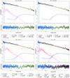 |
Fig. C.1. Spectral fit of RGS + stacked MOS1 (light blue and green points, upper left panel), RGS + stacked MOS2 (light blue and green points, upper right panel), RGS + stacked pn (light blue and green points, lower left panel), and RGS + all stacked EPIC (light blue, green, violet and black points, lower right panel). Residuals are shown in the bottom panel. The model used for fitting is the combination of cie and the isobaric CF split into three temperature intervals. The model components are represented with different colors and line styles in the plots. Orange lines represent the cie component, and blue lines represent the power law component describing the ICM and AGN, respectively. Magenta, gold, and light green lines represent the three temperature bins (0.5-1, 1-2, and 2-3 keV) components. |
All Tables
XMM-Newton data: Total exposure times obtained for each ObsID after data reduction.
Results from EPIC/MOS1, EPIC/MOS2, and EPIC/pn joint fit for the three different ObsID.
XMM-Newton/RGS best-fit MDRs for a CF component with five, three, and two temperature bins.
XMM-Newton/RGS and EPIC joint best-fit isothermal cie model with a CF component with three temperature bins.
All Figures
|
Fig. 1. Chandra and XMM images of A2667’s central region. Left panel: Chandra [0.3−10 keV] image of A2667 in a FoV of ∼6 × 4 arcmin2. Right panel: XMM-Newton/EPIC MOS1+MOS2+pn [0.5−7 keV] image of A2667 in a FoV of ∼6 × 4 arcmin2. The magenta circle in both images shows the spectral extraction region of 0.5 arcmin radius used in XMM/EPIC data analysis. |
| In the text | |
|
Fig. 2. RGS spectrum of A2667 overlaid with an isothermal model of gas in collisional equilibrium (red). Emission lines commonly detected in RGS spectra of CC clusters are labeled at the observed wavelengths. Dotted labels refer to lines from gas below 1 keV. Residuals are shown in the bottom panel. The dotted line in the upper panel represents the background spectrum. |
| In the text | |
|
Fig. 3. RGS and EPIC cooling rates measurements and upper limits. In light blue, dark blue, and cyan, we show RGS values and upper limits on cooling rates obtained from a five-component, three-component and two-component CF model. In magenta, we show the EPIC measurements and upper limit of cooling rate obtained from the three-component CF model reported in Table 2 (see all stacked EPIC ObsID). |
| In the text | |
|
Fig. 4. RGS line spatial broadening computed through the Chandra surface brightness profile and Eq. (2) (black line). The lines show the narrowest Gaussian referring only to the cluster core obtained by fitting two different models with either two (dotted red line) or three (dotted blue line) Gaussian lines. |
| In the text | |
|
Fig. 5. Line spatial broadening computed through the Chandra surface brightness profile and Eq. (2) for A2667 (blue line) and Abell 1835 (red line). The dash-dotted turquoise line and the dashed orange line show the narrowest Gaussian obtained by fitting three Gaussian lines for A2667 and Abell 1835, respectively. |
| In the text | |
|
Fig. 6. Chandra 0.3−10 keV unsharp mask image of A2667. The white arrows are adapted from Giacintucci et al. (2019) and represent the two surface brightness edges found, which may be cold fronts or bubble-like features. |
| In the text | |
|
Fig. 7. Simulation of an A2667 observation with XRISM/Resolve accounting for the GVC. The black dots are data points and the red line is the best-fit isothermal model. The plot is zoomed on the region of the FeXXV-XXVI lines in the observer frame. |
| In the text | |
|
Fig. 8. Simulation of an A2667 observation with ATHENA/X-IFU. The black dots are data points and the red line is the best-fit isothermal model + isobaric CF model in three temperature bins. |
| In the text | |
|
Fig. B.1. Spectral fit of MOS1+MOS2 (light blue and green points) and pn (purple points) data for ObsID 0148990101 (upper left panel), 0900280101 (upper right panel), 0900280201 (lower left panel) and all stacked spectra (lower right panel). Residuals are shown in the bottom panel. The model used for fitting is the combination of cie and the isobaric CF split into three temperature intervals. The model components are represented with different colors and line styles in the plots. Orange lines represent the cie component, and blue lines represent the power law component describing the ICM and AGN, respectively. Magenta, gold, and light green lines represent the three temperature bins (0.5-1, 1-2, and 2-3 keV) components. |
| In the text | |
|
Fig. C.1. Spectral fit of RGS + stacked MOS1 (light blue and green points, upper left panel), RGS + stacked MOS2 (light blue and green points, upper right panel), RGS + stacked pn (light blue and green points, lower left panel), and RGS + all stacked EPIC (light blue, green, violet and black points, lower right panel). Residuals are shown in the bottom panel. The model used for fitting is the combination of cie and the isobaric CF split into three temperature intervals. The model components are represented with different colors and line styles in the plots. Orange lines represent the cie component, and blue lines represent the power law component describing the ICM and AGN, respectively. Magenta, gold, and light green lines represent the three temperature bins (0.5-1, 1-2, and 2-3 keV) components. |
| In the text | |
Current usage metrics show cumulative count of Article Views (full-text article views including HTML views, PDF and ePub downloads, according to the available data) and Abstracts Views on Vision4Press platform.
Data correspond to usage on the plateform after 2015. The current usage metrics is available 48-96 hours after online publication and is updated daily on week days.
Initial download of the metrics may take a while.