| Issue |
A&A
Volume 694, February 2025
|
|
|---|---|---|
| Article Number | A94 | |
| Number of page(s) | 19 | |
| Section | Stellar structure and evolution | |
| DOI | https://doi.org/10.1051/0004-6361/202451046 | |
| Published online | 05 February 2025 | |
Uncovering the invisible: A study of Gaia18ajz, a candidate black hole revealed by microlensing
1
Astronomical Observatory, University of Warsaw, Al. Ujazdowskie 4, 00-478 Warszawa, Poland
2
Faculty of Mathematics and Computer Science, Jagiellonian University, Łojasiewicza 6, 30-348 Kraków, Poland
3
Las Cumbres Observatory, 6740 Cortona Drive, Suite 102, Goleta, CA 93117, USA
4
Institute of Astronomy, Faculty of Physics, Astronomy and Informatics, Nicolaus Copernicus University in Toruń, Grudziądzka 5, 87-100 Toruń, Poland
5
IPAC, Mail Code 100-22, Caltech, 1200 E. California Blvd., Pasadena, CA 91125, USA
6
Research School of Astronomy and Astrophysics, Australian National University, Mount Stromlo Observatory, Cotter Road Weston Creek, ACT 2611, Australia
7
Zentrum für Astronomie der Universität Heidelberg, Astronomisches Rechen-Institut, Mönchhofstr. 12-14, 69120 Heidelberg, Germany
8
Department of Particle Physics and Astrophysics, Weizmann Institute of Science, Rehovot 76100, Israel
9
Astronomical Institute, University of Wrocław, ul. Mikołaja Kopernika 11, 51-622 Wrocław, Poland
10
Sydney Institute for Astronomy (SIfA), The University of Sydney, Physics Road, Sydney 2050, Australia
11
Donald Bren School of Information and Computer Sciences, University of California, Irvine, CA 92697, USA
12
Institute of Astronomy, University of Cambridge, Madingley Road, Cambridge CB3 0HA, United Kingdom
13
University of Bonn, Argelander-Institut für Astronomie, Auf dem Hügel 71, 53121 Bonn, Germany
14
School of Physics, Trinity College Dublin, College Green, Dublin 2, Ireland
15
Institut de Ciències del Cosmos (ICCUB), Universitat de Barcelona (UB), Martí i Franquès 1, E-08028 Barcelona, Spain
16
Departament de Física Quàntica i Astrofísica (FQA), Universitat de Barcelona (UB), Martí i Franquès 1, E-08028 Barcelona, Spain
17
Institut d’Estudis Espacials de Catalunya (IEEC), Esteve Terradas, 1, Edifici RDIT, Campus PMT-UPC, 08860 Castelldefels, Barcelona, Spain
18
ICAMER Observatory of National Academy of Sciences of Ukraine, 27 Acad. Zabolotnoho str., Kyiv 03143, Ukraine
19
Astronomy and Space Physics Department, Taras Shevchenko National University of Kyiv, 4 Glushkova ave., Kyiv 03022, Ukraine
20
National Center “Junior Academy of Sciences of Ukraine”, 38-44 Dehtiarivska St., Kyiv 04119, Ukraine
21
INAF-Osservatorio di Astrofisica e Scienza dello Spazio, Via Gobetti 93/3, I-40129 Bologna, Italy
22
Astronomical Institute of the Academy of Sciences of the Czech Republic (ASU CAS), 25165 Ondrejov, Czech Republic
23
Czech Technical University in Prague, Faculty of Electrical Engineering, Prague, Czech Republic
24
Astronomical Institute, Faculty of Mathematics and Physics, Charles University, V Holešovičkách 2, 180 00 Prague, Czech Republic
25
Research Centre for Theoretical Physics and Astrophysics, Institute of Physics, Silesian University, Bezručovo nám. 13, 746 01 Opava, Czech Republic
26
Department of Space Sciences and Technologies, Akdeniz University, Campus, Antalya 07058, Türkiye
27
TÜBİTAK National Observatory, Akdeniz University Campus, Antalya 07058, Türkiye
28
UKIRT Observatory, Institute for Astronomy, 640 N. A’ohoku Place, University Park, Hilo, Hawai’i 96720, USA
29
School of Physical Sciences, The Open University, Walton Hall, Milton Keynes MK7 6AA, UK
⋆ Corresponding author; This email address is being protected from spambots. You need JavaScript enabled to view it.
Received:
9
June
2024
Accepted:
15
November
2024
Abstract
Context. Identifying black holes is essential for our understanding of the development of stars and can reveal novel principles of physics. Gravitational microlensing provides an exceptional opportunity to examine an undetectable population of black holes in the Milky Way. In particular, long-lasting events are likely to be associated with massive lenses, including black holes.
Aims. We present an analysis of the Gaia18ajz microlensing event reported by the Gaia Science Alerts system. Gaia18ajz is a long-timescale event exhibiting features indicative of the annual microlensing parallax effect. Our objective is to estimate its lens parameters based on the best-fitting model.
Methods. We used photometric data obtained from the Gaia satellite and terrestrial observatories to investigate a variety of microlensing models and calculate the most probable mass and distance to the lens, taking into consideration a Galactic model as a prior. Subsequently, we applied a mass–brightness relation to evaluate the likelihood that the lens is a main sequence star. We also describe the DarkLensCode (DLC), an open-source routine that computes the distribution of probable lens mass, distance, and luminosity employing the Galaxy priors on stellar density and velocity for microlensing events with detected microlensing parallax.
Results. We modelled the Gaia18ajz event and found its two possible models, the most probable Einstein timescales for which are 316−30+36 days and 299−22+25 days. Applying Galaxy priors for stellar density and motion, we calculated a most probable lens mass of 4.9−2.3+5.4 M⊙ located at 1.14−0.57+0.75 kpc, and a less probably mass of 11.1−4.7+10.3 M⊙ located at 1.31−0.60+0.80 kpc. Our analysis of the blended light suggests that the lens is likely a dark remnant of stellar evolution rather than a main sequence star.
Key words: gravitational lensing: micro / stars: black holes / Galaxy: stellar content
© The Authors 2025
 Open Access article, published by EDP Sciences, under the terms of the Creative Commons Attribution License (https://creativecommons.org/licenses/by/4.0), which permits unrestricted use, distribution, and reproduction in any medium, provided the original work is properly cited.
This article is published in open access under the Subscribe to Open model. This email address is being protected from spambots. You need JavaScript enabled to view it. to support open access publication.
1. Introduction
In recent years, the field of black hole astronomy has witnessed significant advancements in the detection and characterisation of stellar-mass black holes (sBHs) (Askar et al. 2024) in our Galaxy. Historically, the identification of sBHs was achieved primarily through X-ray observations of accreting binary systems; see for example Casares et al. (1992), Bahramian et al. (2017), and Corral-Santana et al. (2016). More recently, novel techniques for the detection of sBHs have emerged, which have expanded our understanding of these enigmatic objects. The direct observation of gravitational waves, as demonstrated in landmark events, such as the detection of binary black hole mergers (Abbott et al. 2016, 2017, 2019), has opened new avenues for probing the most massive and elusive BHs of the Universe. Additionally, binary systems with luminous companions, as exemplified by the works of Gomel et al. (2023) and Shahaf et al. (2023) and, in particular, by the discoveries of GaiaBH1 (El-Badry et al. 2022; Chakrabarti et al. 2023), GaiaBH2 (El-Badry et al. 2023; Tanikawa et al. 2023), and GaiaBH3 (Gaia Collaboration 2024), have further enriched our knowledge of sBHs with masses of around 10 M⊙.
Nevertheless, our comprehension of the sBHs population and their evolution has predominantly been investigated through binary systems. To construct a comprehensive picture of the mass spectrum and spatial distribution of sBHs, it has become increasingly crucial to explore and investigate isolated BHs. These solitary BHs can have diverse origins, including the remnants of massive single stars (Belczynski et al. 2020; Pejcha & Thompson 2015), disruptions of binary systems (Wiktorowicz et al. 2019), or ejections from globular clusters (Giersz et al. 2022; Leveque et al. 2023).
One promising avenue for the study of solitary sBHs relies on gravitational microlensing. This gravitational phenomenon, a consequence of Einstein’s general theory of relativity, occurs when a massive object passes in front of a distant star within the Milky Way or its vicinity (Einstein 1936; Paczynski 1986). Unlike strong gravitational lensing, where multiple, distorted images of a source can be observed, images in microlensing events are typically almost impossible to resolve. Nevertheless, the very first successful attempts used optical interferometry (Dong et al. 2019; Cassan 2023), revealing a temporary brightening of the background source coupled with a positional shift in the source’s centroid, a phenomenon referred to as astrometric microlensing (Dominik & Sahu 2000; Belokurov & Evans 2002).
Astrometric microlensing, although challenging to observe, has been successfully captured with precise observatories such as the Hubble Space Telescope (HST) (Sahu et al. 2017; McGill et al. 2023). The combination of astrometric and photometric microlensing effects can be leveraged to determine the mass of the lensing object (ML) (Gould 2000). The formula used for this purpose is derived from the angular Einstein radius (θE) and the microlensing parallax (πE). Remarkably, this technique recently led to the direct measurement of the mass of a solitary sBH for the first time (Sahu et al. 2022; Lam et al. 2022), opening a new channel for study of stellar evolution and BH production (Andrews & Kalogera 2022; Horvath et al. 2023; Vigna-Gómez & Ramirez-Ruiz 2023).
The European Space Agency’s Gaia mission (Gaia Collaboration 2016) is going to be a valuable asset for astrometric microlensing studies due to its long-term all-sky submilliarcsecond accuracy of epoch astrometric measurements for nearly 2 billion stars (Rybicki et al. 2018). Gaia has proven to be capable of detecting microlensing events in its time-domain photometric data. In its latest data release, Gaia DR3 contained a catalogue of microlensing events from all over the sky (Wyrzykowski et al. 2023). Another source of microlensing events is the near-real-time system of Gaia Science Alerts (GSA) (Wyrzykowski et al. 2012; Hodgkin et al. 2013, 2021), which detects ongoing events and alerts the astronomical community.
Here we present an analysis of one of the GSA alerts, Gaia18ajz, which was one of the longest microlensing events ever studied. Long-lasting microlensing events are thought to be the most likely result of massive lenses, as their large timescale could be related to a large Einstein radius, with prior examples presented in Mao et al. (2002) and Kruszyńska et al. (2022). However, the lack of an Einstein radius measurement for this event has so far prevented the derivation of the mass of the lensing object. Nevertheless, such events typically exhibit the microlensing parallax effect (Gould 2000), which, when combined with information on the Galaxy and the possible kinematics of the lenses, can provide a means to estimate the most likely mass and distance of the lens (e.g. Wyrzykowski et al. 2016; Wyrzykowski & Mandel 2020; Mróz & Wyrzykowski 2021). In this work, we present the DarkLensCode (DLC), which is open-source software for generating posterior probability distributions for the physical parameters of the lens using microlensing parallax posteriors obtained from a light curve.
2. Discovery and ground-based observations of Gaia18ajz
Gaia18ajz (AT2018uh according to the IAU transient name server) was discovered by Gaia Science Alerts on February 9, 2018 (HJD′ = HJD – 2450000.0 = 8159.09). On February 14, it was posted on the GSA website1. The event was located at equatorial coordinates right ascension(RA)J2000 = 18h30m14.46s, declination(Dec)J2000 = −08°13′12.76″ and galactic coordinates l = 23.20506° , b = +0.925751°. The finding chart with the location of the event in the sky is presented in Figure 1.
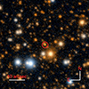 |
Fig. 1. Location of Gaia18ajz and its neighbourhood during the event. The image comes from Pan-STARRS DR1 via the Aladin Tool implemented in BHTOM. |
Gaia Data Release 2 (GDR2) (Gaia Collaboration 2018) and Gaia Data Release 3 (GDR3) (Gaia Collaboration 2023) contain an entry for this source under Gaia Source ID = 4156664130700362752. Astrometric parameters for this object from both GDR2 and GDR3 are presented in Table 1.
Gaia astrometric parameters for the source star in Gaia18ajz.
2.1. Gaia photometry
The Gaia photometic data are collected in a wide G-band (Jordi et al. 2010). As of March 2024, Gaia has collected 86 measurements for Gaia18ajz and the event has returned to its baseline. The light curve obtained by Gaia has one peak reaching about 17.6 mag in the G band and a baseline of around 19.3 mag in the same band.
The GSA system does not provide errors of magnitude for published events. In order to estimate these error bars, we followed a method described previously in Kruszyńska et al. (2022). The error bars for this event should vary from 0.02 mag for G = 17.6 at peak to 0.06 mag for G = 19.3 at baseline.
2.2. Ground-based photometric observations
Consistent photometric follow-up is essential in order to obtain accurate values for the best-fitting microlensing model, particularly blending parameters. This involves observation of the event not just at its peak brightness but also during the baseline using the same telescope. Due to the fact that the event was faint, especially at its baseline, with G = 19.3 mag, the follow-up data are affected by a large measurement error.
Following the event announcement on the GSA website, the earliest follow-up began 13 days later. The first data point was taken on 22 February 2018, by Paweł Zieliński using a 1.3 m SMARTS telescope equipped with the ANDICAM instrument at Cerro Tololo Inter-American Observatory, Chile. Additional observations were also carried out with: the 0.8 m Joan Oró Telescope using MEIA2 CCD at Montsec astronomical observatory, Spain (ObsMontsec); the 1.52 m Loiano telescope with BFOSC, Italy (Loiano); the 0.6 m PIRATE (Physics Innovations Robotic Astronomical Telescope Explorer) telescope of the Open University in the UK, with FLI ProLine KAF-16803 camera, on Tenerife, Spain; the 2 m Terskol with the FLI PL4301 camera and 0.6 m Terskol with the SBIG STL1001E camera in the North Caucasus operated by the National Academy of Sciences of Ukraine; the 2 m Ondrejov Telescope in Czechia (Ondrejov); the 0.6 m T60 robotic telescope with FLI Proline3041 at TÜBÍTAK National Observatory, Turkey (TUG T60); and the 1.54 m Danish Telescope in La Silla, Chile. The number of data points observed by each observatory is presented in Table 2. All data points are visible in the Figure 2. Ground-based observations were reduced using the automatic tool for time-domain data, the Black Hole TOM (BHTOM) tool2. The bias-, dark-, and flat-field-corrected images were processed to obtain instrumental photometry for all stars in the image. The photometry was then calibrated as described in Zieliński et al. (2019, 2020) to the Gaia Synthetic Photometry magnitudes (Montegriffo et al. 2023).
Photometric data collected for Gaia18ajz from different observatories.
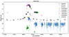 |
Fig. 2. Photometric data collected for Gaia18ajz. The different colours represent different bands. |
The Zwicky Transient Facility (ZTF) is an astronomical survey designed to detect transient and variable objects in the sky through repeated observations using a wide-field camera mounted on the Samuel Oschin Telescope at the Palomar Observatory (CITE). ZTF observed this target serendipitously while scanning the Northern sky. ZTF provides data in r- and g-band openly; however, only r-band data were collected during the actual event in 2018.
The event was also observed by the Optical Gravitational Lensing Experiment (OGLE; Udalski et al. 2015) as part of its Galaxy Variability Survey (Mróz et al. 2020) from May 2015 to October 2019. OGLE uses a 1.3 m Warsaw Telescope located at Las Campanas Observatory, Chile. All OGLE observations were collected through an I-band filter and were reduced using the standard OGLE pipeline (Udalski et al. 2015).
2.3. Spectroscopic follow-up
The object was also observed spectroscopically with the X-shooter instrument (Vernet et al. 2011) mounted on the ESO Very Large Telescope (VLT). The first spectrum was obtained on 25 March and the second on 8 August 20183. The following setup was applied: the slit width 1.0 arcsec, 0.7 arcsec, and 0.6 arcsec for UVB (300 − 559.5 nm), VIS (559.5 − 1024 nm), and NIR (1024 − 2480 nm) channels, respectively, and exposure times of 1872 s (UVB), 2104 s (VIS), and 2400 s (NIR) for both spectra. This gave us the resolution of R ∼ 4300 and the median signal-to-noise ratio S/N = 0.2 in UVB, and R ∼ 10 500 and S/N = 29 in VIS, and R ∼ 7900 and S/N = 188 in NIR for the first spectrum, while for the second spectrum we obtained R ∼ 4300 and S/N = 0.3 in UVB, R ∼ 10 500 and S/N = 37 in VIS, and R ∼ 7900 and S/N = 243 in the NIR part.
X-shooter data were reduced in a standard way using the EsoReflex4 pipeline. The ThAr comparison lamp was used for the calibration of UVB and VIS wavelengths, and the Ar, Hg, Ne, and Xe lamps were used for NIR wavelengths.
The first spectrum was used to classify this target as a microlensing event that was published in Kruszynska et al. (2018). The spectrum did not present emission features and only absorption lines, and the continuum shape indicated a late-type star with significant reddening. This ensured that we were able to continue ground-based photometric follow-up of the Gaia18ajz event.
3. Photometric microlensing model
In this paper, following the procedure described previously in Kruszyńska et al. (2022), we fit two single-source and single-lens models: with and without taking into account the annual parallax effect (e.g. Wyrzykowski et al. (2016), Kaczmarek et al. (2022), Jabłońska et al. (2022)).
3.1. Standard model
The first is the standard Paczyński light-curve model described in Paczynski (1986). It is defined by the following parameters:
-
t0: Time of peak brightness.
-
u0: Impact parameter, defined as the source-lens separation in units of the Einstein radius at time t0.
-
tE: Timescale, defined as θE/μLS, where μLS is the relative proper motion of the source and the lens.
-
mag0: Baseline magnitude, calculated separately in each of the observing bands, and defined as mag0 = −2.5log(FS + FB), where FS is the baseline flux of the source and FB is the baseline flux of the blend.
-
fS: Blending parameter, defined as part of the flux coming from the source star (separately in each of the observing bands), and defined as
 .
.
3.2. Parallax model
As the event studied was extremely long, we have to consider the Earth’s movement around the Sun. The second model considered, described in Gould (2000) and Gould (2004), is an extension of the Paczyński model that takes into account the annual parallax effect. In this model, in addition to the parameters described above, we include two additional parameters: πEN and πEE. These parameters are, respectively, the (equatorial) north and east components of the microlensing parallax πE, projected in the direction as the relative proper motion of the lens and the source.
3.3. Modelling and results
Due to the relatively low brightness of the event and the resulting large scatter in the ground-based data, we decided to fit three sets of models. The first set was trained using only Gaia data, and the second set was trained using both the Gaia data and ground-based data. We decided to only use data from ZTF, OGLE, and SMARTS facilities. In addition, we trained the third set using photometric data from Gaia and OGLE, which are of the best quality.
We used a Markov chain Monte Carlo (MCMC) method to explore the parameter space of the microlensing models described above. The models were trained using MulensModel (Poleski & Yee 2019) with the emcee package (Foreman-Mackey et al. 2013). During modelling, we scaled the error bars separately for each model and each band so that χ2 per degree of freedom for every band is equal to one. In order to ensure that models are physical, we introduced a Gaussian prior on negative flux:
 (1)
(1)
for Fb < 0, where Fb is the blended flux. A flux equal to 1 corresponds to 22 mag.
To ensure that all possible solutions were uncovered and the entire parameter space was explored, we visually examined the MCMC results. In all sets of models, all posterior distributions were found to be bimodal, with classic degeneracy with respect to the impact parameter. This degeneracy is caused by the fact that the lens can pass in front of the source from both sides, resulting in a change of sign in the impact parameter. We decided to divide bimodal solutions into two separate models, one with a positive and the other with a negative impact parameter u0 and to model them separately. Finally, our results contain nine different models:
-
G0 : Gaia-only, no-parallax.
-
G+ : Gaia-only, parallax, positive u0.
-
G- : Gaia-only, parallax, negative u0.
-
GG0 : Gaia+ground, no-parallax.
-
GG+ : Gaia+ground, parallax, positive u0.
-
GG- : Gaia+ground, parallax, negative u0.
-
GO0 : Gaia+OGLE, no-parallax.
-
GO+ : Gaia+OGLE, parallax, positive u0.
-
GO- : Gaia+OGLE, parallax, negative u0.
In the case of the standard model without taking into account the parallax effect, we decided to report only one solution with a positive impact parameter. Due to the lack of the parallax effect, the solution with a negative impact parameter is symmetrical. Additionally, to test which of the two modes of posterior distribution is more likely, we analysed the event using nested sampling with nested_ulens_parallax code5 (Kaczmarek et al. 2022; Speagle 2020).
Table 3 displays the optimal parameter values obtained using only Gaia data, while Table 4 presents the optimal parameter values obtained using both Gaia and all ground-based follow-up photometric data. Table 5 shows the results of the modelling for GO models. For each band, the baseline magnitude and blending parameters were determined independently. As a reference for calculating χ2/d.o.f., we decided to use the data set used to model the GG+ model, with error bars rescaled according to this model.
Optimal parameter values for fitting Gaia18ajz using only Gaia photometric data.
Optimal parameter values for fitting Gaia18ajz using both Gaia and ground-based follow-up photometric data.
Optimal parameter values for fitting Gaia18ajz, using Gaia and OGLE photometric data.
Figures 3, 4, and 5 show light curves for all models for the Gaia-only, Gaia+follow-up, and Gaia+OGLE datasets, respectively. The corner plots are available in Appendix B.
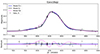 |
Fig. 3. Light curve of the Gaia18azj event and the microlensing model fit using only the Gaia data. The dashed magenta line represents the model without parallax, while the blue and black solid lines show the positive and negative solutions for the parallax model, respectively. The bottom panel shows the residuals with respect to the negative solution for the parallax model. |
 |
Fig. 4. Light curve of the Gaia18azj event and the microlensing model fit using the Gaia data as well as the ground-based survey data from ZTF, SMARTS, and OGLE. The dashed magenta line represents the model without parallax, while the blue and black solid lines show the positive and negative solutions for the parallax model, respectively. The bottom panel shows the residuals with respect to the negative solution for the parallax model. |
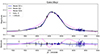 |
Fig. 5. Light curve of the Gaia18azj event and the microlensing model fit using the Gaia data as well as the ground-based data from OGLE. The dashed magenta line represents the model without parallax, while the blue and black solid lines show the positive and negative solutions for the parallax model, respectively. The bottom panel shows the residuals with respect to the negative solution for the parallax model. |
Table 6 shows the equal-weight sample ratio of the solution with positive impact parameter to the solution with negative impact parameter u0 for Gaia-only and Gaia + OGLE models. Ratios were obtained using nested sampling.
Equal-weight sample ratios of the solution with positive impact parameter to the solution with negative impact parameter u0.
4. Source star
4.1. Atmospheric parameters
In order to obtain the atmospheric parameters of the source star of the Gaia18ajz event, we performed the spectral analysis with the iSpec6 framework of various radiative transfer codes (Blanco-Cuaresma et al. 2014; Blanco-Cuaresma 2019). The effective temperature Teff, surface gravity log g, and metallicity [M/H] were determined using the SPECTRUM7 code, a grid of MARCS atmospheric models (Gustafsson et al. 2008), solar abundances from Grevesse et al. (2007), and the atomic line list from the Gaia-ESO Survey (GESv6; Heiter et al. 2021). The GESv6 line list covers the wavelength range from 420 to 920 nm, and therefore only the UVB and VIS part of the X-shooter spectra could be used. However, due to the poor quality and low S/N of the UVB region in both spectra, we decided to fit the synthetic spectra for the VIS part only. We obtained the Teff, log g, and [M/H] of the source star in both cases. The final solutions of the atmospheric parameters resulting from the fitting procedure of both X-shooter spectra are presented in Table 7 and Fig. 6.
Parameters of the source star determined via synthetic spectrum fitting and template matching.
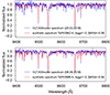 |
Fig. 6. Result of the synthetic spectrum fitting (red spectra) to the X-shooter spectroscopic data (blue spectra) generated for the best-matching atmospheric parameters. The Ca II triplet region is presented for two spectra obtained in 2018, March 25 (top panel) and August 8 (bottom panel) by using X-shooter. |
In addition to the absorption line analysis, we applied a template-matching method using Spyctres8, similarly to Bachelet et al. (2022). We modelled both X-shooter spectra using the stellar template library from Kurucz (1993) as well as the spectral energy distribution (SED) at the time of spectra acquisition, including the source magnification A(t)∼5 (for the first spectrum) and A(t)∼4 (for the second spectrum). We used MCMC (Foreman-Mackey et al. 2013) sampling in order to generate the chains for final values of the effective temperature Teff, the surface gravity logg, the metallicity [Fe/H], the radial velocity of the source star, the angular source radius θ* and the line-of-sight extinction AV. We constrained MCMC chains using the mean values of the parameters obtained in synthetic spectra fitting as input values. As a result, we obtained the stellar parameters and the line-of-sight extinction AV thanks to an accurate flux calibration in the wide wavelength range of X-shooter data (UVB+VIS+NIR parts) and the updated extinction law taken from Wang & Chen (2019). The extinction parameter AV was additionally constrained by taking into account the unblended apparent V magnitude. The final values of parameters obtained in template matching are presented in Table 7 (last column) and in Fig. 7.
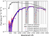 |
Fig. 7. Two spectra from VLT/X-shooter obtained in March 25 (red) and August 8 (blue), 2018, as well as the best models with (solid lines) and without (dashed lines) extinction correction. The grey vertical lines and regions indicate the telluric bands, where the data were not used for the modelling. |
Based on the parameters determined in these two methods, we state that the Gaia18ajz source is a reddened K5-type supergiant or bright giant (luminosity class I or II) located in the Galactic disc. Schlegel et al. (1998) and Schlafly & Finkbeiner (2011) estimated the value of AV to be as high as 11.76 mag and 10.11 mag, respectively, assuming a visual extinction to reddening ratio of AV/E(B − V) = 3.19. High reddening for this location in the Galaxy is confirmed by the Galactic dust distribution, which is in agreement with the value obtained by us of AV = 7.3 mag.
4.2. Distance
The atmospheric parameters and exctinction AV in the direction to the Gaia18ajz event were used to calculate the distance to the source from the equation
 (2)
(2)
where DS is the distance to the source star, V is the apparent magnitude, MV is the absolute magnitude, and AV is the interstellar line-of-sight extinction. Assuming the typical absolute magnitude of MV = −1.4 ± 0.2 mag for the metal-poor K5 I/II star estimated using CMD 3.710 with PARSEC (v1.2S) isochrones (Bressan et al. 2012), as well as the apparent brightness of V = 21.82 ± 0.05 mag, we obtain a distance to the source star of DS = 15.26 ± 2.46 kpc.
Moreover, the template-matching analysis yields a source distance distribution based on PARSEC isochrones, which is presented in Fig. 8. According to this distribution, the average distance to the source of the Gaia18ajz event is 13.75 ± 1.02 kpc. This value is in agreement with the spectroscopic distance calculation within 1σ uncertainty. The plot also shows that the source is located in the region of the Kiel diagram (logg − log Teff) where isochrones for ages of > 4 Gyr are dominant, assuming metal-poor stars.
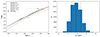 |
Fig. 8. (Left) PARSEC stellar isochrones for 1.3, 2.2, 4.0, 7.1, and 12.6 Gyr with a fixed metallicity of −0.5. The source is most likely an old bright giant or supergiant. (Right) Source distance distribution based on PARSEC isochrones and the extinction estimated from the spectral modelling. Black dashed and dotted lines indicate the median distance value and the 1σ confident region, respectively. |
The spectroscopic distances obtained according to the above-mentioned approach are inconsistent with distances based on the Gaia parallax measurements. Bailer-Jones et al. (2021) inferred the distance to Gaia18ajz by taking into account astrometric (geometric model) and astrometric + photometric measurements (photogeometric model) published in GaiaDR3 (Gaia Collaboration 2023), finding  kpc when assuming the geometric model and
  kpc when assuming the photogeometric model, which are 4.5 and 3.5 times smaller than our spectroscopic value, respectively. Moreover, Bailer-Jones et al. (2018) inferred an even smaller value of the distance of
  kpc based on GaiaDR2 data (Gaia Collaboration 2018). The reason for such a discrepancy in the distance can be explained with the help of the astrometric quality flags published in the Gaia archive and presented in Table 1. First of all, the RUWE parameter in both data releases is higher than 1.4, which is the tolerance limit according to the Gaia Data Processing and Analysis Consortium (DPAC) documentation11. This could indicate that the astrometric solution for the source is problematic due to the large scatter in the measurements or the binary nature of the object. Another parameter that provides a consistent measure of the astrometric goodness-of-fit is astrometric_excess_noise, which is also relatively high in the case of Gaia18ajz, with a value of 3.1 mas (for GaiaDR3). Because we do not see any evidence of the binarity in the light curve or in the spectroscopic data, we suspect that Gaia measurements were affected by either some instrumental effects or centroid shift motion due to the astrometric microlensing. In addition, it is clearly visible that the parallaxes and proper motions, both in the GaiaDR2 and DR3 releases, are characterised by relatively high 1σ error bars. These yield small values of the parameter parallax_over_error, of namely 5.49 (for GaiaDR2) and 2.81 (for GaiaDR3), and reveal the low quality of the Gaia measurements for Gaia18ajz. The large scatter of the astrometric data and indications of problems with obtaining a reliable solution lead us to distrust the Gaia astrometric parallax measurement in this case. Therefore, we decided to use the spectroscopic distance as the main constraint for lens mass and distance in the microlensing model.
5. Lensing object
5.1. Assumptions
As there are no available astrometric data for this event, determining the exact values of the distance to the lens and its mass is currently impossible. To uncover the most likely parameters of the lens relying solely on photometric data, we employed the DarkLensCode described in detail in Appendix A.
As the G filter is wider than the V filter, we assumed the upper bound of extinction to the lens to be AG = 7.3 mag, which is the value of extinction to the source star in the V filter derived from spectroscopy. Following Kaczmarek et al. (2022), for the lower bound, we assumed AG = 0 mag. For the proper motion of the source star, we assumed the values of Gaia DR3 shown in Table 1, despite the elevated RUWE value in Gaia catalogues. The proper motions reported in GDR2 and GDR3 are consistent with each other to within error bars, while the reported parallaxes are very different. For the source distance, we assumed the value from spectroscopy and, at each iteration of the code, we drew DS from the normal distribution with a mean of 15.26 kpc and a standard deviation of 2.46 kpc. We used two mass functions as lens mass priors. First, the Kroupa (2001) initial mass function (IMF; hereafter StellarIMF) describes stellar objects,
 (3)
(3)
and second, the Mróz et al. (2021) IMF (hereafter DarkIMF) describes solitary dark remnants in the Milky Way:
 (4)
(4)
A summary of the input parameters for the DarkLensCode is shown in Table 8.
DarkLensCode input parameters.
5.2. Mass and distance
To estimate the mass and distance of the lens, we employed samples from MCMC models of both the GO+ and GO- models. Figure 9 shows the two-dimensional posterior distribution of the lens mass and lens distance. Figure 10 shows the posterior distribution of the blend magnitude and lens magnitude in the hypothetical case where the lense is a main sequence star. Both figures come from the GO− photometric model and assume the StellarIMF.
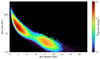 |
Fig. 9. DarkLensCode output for the GO+ microlensing model assuming the DarkIMF. This diagram shows the posterior distribution of the distance to the lens and its mass. The colours correspond to the log probability density. The dark color of a bin means that there were no samples present in this bin. |
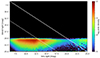 |
Fig. 10. DarkLensCode output for the GO+ microlensing model assuming the StellarIMF mass function. Posterior distribution of the blended light magnitude and lens light magnitude assuming that the lens is an MS star. The solid line represents the upper limit of extinction, while the dashed line represents the lower limit of extinction. Lines separate the dark lens solutions from the MS star solutions. The colours correspond to the log probability density. Black bins are those containing no samples. |
As can be seen in Figure 9, the posterior distribution is bimodal with two distinct solutions. One represents a more massive, close lens while the other is less massive and is at a greater distance. We decided to split these solutions at DL = 5 kpc. Assuming the mass function for luminous sources (StellarIMF), we estimated the dark lens probability (DLProb) and the probability of each solution (defined as the sum of the weights in each solution divided by the sum of all weights). As the DLProb of more massive solutions is high, we recalculated all weights using the DarkIMF. We report ML, DL, θE, and the solution probability for both mass functions. As the calculation of the dark lens probability assumes that the lens is a MS star, we report the DLProb using only the StellarIMF. The results for the GO- photometric model are shown in Table 9, while the results for the GO+ photometric model are in Table 10.
DarkLensCode output for the GO- solution for each possible scenario. Estimations for the lens distance and mass, as well as θE, and the probability of the lens being a dark remnant for each possible scenario.
DarkLensCode output for the GO+ solution for each possible scenario. Estimations of the lens distance and mass, as well as θE, and the probability of the lens being a dark remnant.
6. Discussion
The Gaia18ajz microlensing event lasted about 1000 days, making it one of the longest microlensing events ever studied. The most probable explanation for the light curve shape is that it is the result of microlensing caused by a single lens on a single source with a visible annual parallax effect. The standard Paczyński model without the inclusion of the parallax effect, which is visible in Figures 3, 4, and 5 as a dashed line, cannot fully explain the changes in magnitude. The light curve does not show any features due to binarity of the lens, such as caustic crossings in particular, and therefore we can immediately rule out binary lenses with separations of the order of 1AU. The effect of space parallax was not included in the models obtained. Due to significant measurement error caused by the low brightness of the event, as well as the small annual parallax effect, we can assume that space parallax has minimal effect on the light curve.
The event was observed by various observatories (Table 2, Figure 2). However, due to the low brightness of the event, at a baseline below 19 mag in G and below 21 mag in V, most of the data are affected by significant measurement errors. Datasets from Gaia and OGLE are of the best quality. Although the data from other observatories have bigger error bars, they are consistent with the data from Gaia and OGLE.
High-resolution spectroscopic observations were possible around the maximum of the Gaia18ajz brightness. We used the VLT/X-shooter instrument at two epochs when the factor of amplification of the source was greatest: approximately a factor five in the case of the first spectrum and about a factor four in the case of the second spectrum. Because of this, we were able to determine the atmospheric parameters of the source, the line-of-sight extinction, and the spectroscopic distance. Based on spectral analysis, the Gaia18ajz source was classified as a reddened K5 supergiant or a bright giant at a large distance of 15.26 kpc. The spectroscopic parameters, especially the distance, constrained the microlensing models and helped in estimates of the lens distance and mass as well as the probability of the lens being a dark remnant.
The event can be explained by two models, one with a positive impact parameter and another with a negative impact parameter u0. Models obtained using only data from Gaia (G models), data from Gaia and OGLE (GO models), and data from Gaia and all of the ground-based follow-up (GF models) agree with each other within error bars. Although the differences are not large, the GO+ model has the lowest χ2 of all the models. The discrepancy between the two solutions cannot be resolved with the available photometric data. The model with a positive impact parameter is more likely than the model with a negative impact parameter. In the case of Gaia + OGLE models, GO+ is 24.68 times more likely than GO-.
Estimates of the distance to the lens and its mass obtained using DarkLensCode indicate two possible scenarios. In the first scenario, the lens is closer and has a greater mass, whereas in the alternate scenario, the lens is situated farther away and has a smaller mass. Based on calculations by DarkLensCode, the probability that the lens is a dark remnant exceeds 79.6% in the more massive scenario, while in the second scenario, this probability falls below 32.7% for the more probable GO+ model. For the GO- model, in the more massive case, the lens is a dark remnant object in more than 99.5% of outcomes. In the less massive case, this probability is between 4.8% and 98.0%. Estimates of the distance to the lens and its mass are highly dependent on the assumed mass function.
If we assume that the lens is a star and the mass function is defined by Equation (3) (Kroupa 2001) (StellarIMF), for a less massive solution we get  located at
  for the GO- model and
  at
at  for the GO+ model. Regardless of extinction, for the GO- model the lens is unlikely to be a star and to belong to the more massive solution. For the more likely GO+ model, if the extinction is close to the maximal value, the GLProb of the model is close to 85%, which means there is a 15% chance of the lens being a MS star with
  at
at  . In the remaining 85% of outcomes, the lens is a dark remnant, which contradicts our assumption of the StellarIMF.
If we assume that the lens is a dark remnant, and the mass function is defined by Equation (4) (Mróz et al. 2021) (DarkIMF), for the more massive solution we obtain  located at
  for the GO- model and
  at
at  for the GO+ model. In this scenario, the lens is likely a sBH. For a model with a positive impact parameter, the less massive solution is highly improbable. However, if the extinction were in the lower half of the possible range, the GLProb for the GO- model would be in the higher half of the possible range. In that case, the lens would have a mass of
  at a distance of
  . This would classify the lens as a massive white dwarf or a light neutron star.
The assumed distance to the source star affects the lens mass and the distance estimates obtained. A small distance, such as  from GDR3, would result in a closer lens, which would eliminate the less massive solution provided by DarkLensCode. In such a case, if the lens were an MS star, the lens would be bright enough to be visible, which is in disagreement with the blending parameter. A greater distance to the source star would result in a greater distance to the lens and a lower lens mass.
In the DarkLensCode analysis, we assume that the proper motion given by Gaia DR3 represents the proper motion of the source star. The microlensing event occurred after the time period within which data were collected for GDR2 (2014.5–2016.4), and so it could not have influenced the measurement of proper motion in GDR2. Furthermore, the proper motion values from Gaia DR2 and Gaia DR3 (2014.5–2017.4) agree with each other within the error bars. As the proper motion signal is stronger than the parallax signal and grows over time as the star moves, the proper motion should be measured accurately, even if the parallax is not and the RUWE is elevated. In this case, the high RUWE is probably not caused by the microlensing event alone (as discussed further); it could be the result of a single erroneous measurement, which should not significantly affect the proper motion measurement. This is justification for our choice to use the proper motion from Gaia as the proper motion of the source star, in addition to the almost negligible blended light. Moreover, our experiments with DarkLensCode showed that using random proper motion values from a Gaussian distribution – with medians matching the GDR3 measurements – does not significantly change the result but instead makes the observed degeneracy more diffuse.
The possibility that the Gaia18ajz lens is a sBH becomes apparent when comparing the measured tE and πE parameters from all parallax solutions with the distributions of typical timescales and parallaxes for microlensing events. Figure 11 shows the location of Gaia18ajz solutions within the microlensing parameter space for stars, neutron stars, and BHs as computed by Kaczmarek et al. (2024). Notably, the Gaia18ajz solutions fall in a region where BHs dominate. It is also worth highlighting that the only known isolated BH to date, OB110362 (Sahu et al. 2022; Lam et al. 2022; Mróz et al. 2022; Lam & Lu 2023), is situated close to Gaia18ajz in this parameter space.
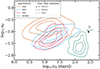 |
Fig. 11. Location of all parallax solutions for Gaia18ajz photometry superimposed on the distribution of tE and πE parameters expected for microlensing events using the simulated data from Kaczmarek et al. (2024). |
The Gaia astrometric time series is currently unavailable and will not be accessible until the publication of Gaia Data Release 4 in 2026. However, Gaia DR2 (Gaia Collaboration 2018) and Gaia DR3 (Gaia Collaboration 2023) reported the astrometric parameters of the object associated with Gaia18ajz (Source ID = 4156664130700362752 in both releases), as shown in Table 1. Gaia DR3, in particular, used the Gaia astrometric time series from 25 July 2014 (10:30 UTC) to 28 May 2017 (08:44 UTC) (up to JD = 2457890.86389). Gaia18ajz was discovered on 14 February 2018, but the photometric deviation began before JD = 2457800. As shown in Belokurov & Evans (2002), the astrometric microlensing signal becomes significant around  , which is approximately two times tE before the peak of the event. However, the elevated value of the RUWE parameter (Lindegren et al. 2018) indicates that the fit of the six-parameter astrometric model to the astrometric data has significant residuals. Furthermore, the value of the parallax (3.24 ± 0.59 mas and 1.52 ± 0.54 for GDR2 and GDR3, respectively) is far from the expected value for the source distance we find with spectroscopy. Although the astrometric microlensing effect could cause the RUWE to grow from 1.49 in GDR2 to 1.53 in GDR3, it cannot explain all the anomalies in the astrometric fit. Using the Astromet code12 and applying the method of Jabłońska et al. (2022), we conclude that the θE needed to reproduce the parallaxes of GDR2 and GDR3 would cause the separation of the images to be high enough for Gaia to detect them as separate sources. We can therefore assume that some other effect must be responsible for the disagreement in parallax and high RUWE in Gaia DR2 (and in GDR3).
If it were confirmed that the lens is a BH, this would be the second known isolated BH. The only currently known isolated BH was discovered by Sahu et al. (2022) and Lam et al. (2022). If the mass of the BH in Gaia18ajz event were equal to  as in the GO+ solution, it would be the lightest isolated BH currently known. According to Mróz et al. (2022), the only currently known isolated BH has a mass of 7.88 ± 0.82 M⊙. In this case, the Gaia18ajz lens is also most likely lighter than the previously detected Gaia BHs, namely GaiaBH1 with a mass of 9.62 ± 0.18 M⊙ (El-Badry et al. 2022; Chakrabarti et al. 2023), GaiaBH2 with a mass of 8.9 ± 0.3 M⊙ (El-Badry et al. 2023; Tanikawa et al. 2023), and GaiaBH3 with 33 M⊙ (Gaia Collaboration 2024). On the other hand, the GO- solution yields a mass of
  , which would make Gaia18ajz the most massive non-interacting single BH known so far.
7. Conclusions
In this work, we present our investigation and analysis of a long microlensing event Gaia18ajz located towards the Galactic disc discovered by the Gaia space satellite. The event exhibited a microlensing parallax effect perturbed by the Earth’s orbital motion. Our investigation is based on Gaia data and ground photometry, as well as spectroscopy follow-up observations. The event has two best-fitting solutions, one with a negative impact parameter and the other with a positive impact parameter, u0. The latter model is more likely. The parameters of these solutions are presented in Tables 3, 4, and 5.
Using DarkLensCodeA, we estimated the probability density of the lens mass and distance. We find two possible scenarios, one closer and more massive, and one further and less massive. We present the results in Tables 9 and 10. We conclude that in the more massive scenario, the lens is a BH with a mass of  at
at  for the less probable model and
  at
at  for the more probable photometric microlensing solution. For the less massive solution, we obtain a white dwarf or a star with a mass of
  at
at  or
or  at
at  . The final Gaia Data Release DR4 (2026), with astrometric time series data for the Gaia18ajz source, could address the issue of elevated RUWE and possibly resolve the ambiguity between near- and far-recognition scenarios, and could be used to confirm which photometric solution is correct.
ESO Programme ID: 0101.D-0035(A), PI: Ł. Wyrzykowski.
Acknowledgments
The authors would like to thank Dr Radek Poleski for discussion and his comments during the creation of this work. This work has made use of data from the European Space Agency (ESA) mission Gaia (https://www.cosmos.esa.int/gaia), processed by the Gaia Data Processing and Analysis Consortium (DPAC, https://www.cosmos.esa.int/web/gaia/dpac/consortium). Funding for the DPAC has been provided by national institutions, in particular the institutions participating in the Gaia Multilateral Agreement. The project has received funding from the European Union’s Horizon 2020 research and innovation programme under grant agreement No. 101004719 (OPTICON RadioNet Pilot, ORP). BHTOM acknowledges the following people who helped with its development: Patrik Sivak, Kacper Raciborski, Piotr Trzcionkowski, and AKOND company. This paper made use of the Whole Sky Database (wsdb) created by Sergey Koposov and maintained at the Institute of Astronomy, Cambridge by Sergey Koposov, Vasily Belokurov and Wyn Evans with financial support from the Science & Technology Facilities Council (STFC) and the European Research Council (ERC), with the use of Q3C software (http://adsabs.harvard.edu/abs/2006ASPC..351..735K). This research has used the VizieR catalogue access tool, CDS, Strasbourg, France. We acknowledge also the use of ChatGPT3.5 from OpenAI, which was helpful as a tool to improve the text of some parts of the manuscript, aiming to mitigate any potential impact of non-native language usage on the overall quality of the publication. In particular, the title of the work, the abstract, and portions of the introduction were generated collaboratively with the aid of ChatGPT. Additionally, the description of the data was automatically generated using the BHTOM ver.2.0 Publication feature. J. M. Carrasco was (partially) supported by the Spanish MICIN/AEI/10.13039/501100011033 and by “ERDF A way of making Europe” by the “European Union” through grant PID2021-122842OB-C21, and the Institute of Cosmos Sciences University of Barcelona (ICCUB, Unidad de Excelencia ‘María de Maeztu’) through grant CEX2019-000918-M. The Joan Oró Telescope (TJO) of the Montsec Observatory (OdM) is owned by the Catalan Government and operated by the Institute for Space Studies of Catalonia (IEEC). ZK is a Fellow of the International Max Planck Research School for Astronomy and Cosmic Physics at the University of Heidelberg (IMPRS-HD).
References
- Abbott, B. P., Abbott, R., Abbott, T. D., et al. 2016, Phys. Rev. Lett., 116, 061102 [Google Scholar]
- Abbott, B. P., Abbott, R., Abbott, T. D., et al. 2017, Phys. Rev. Lett., 118, 221101 [CrossRef] [Google Scholar]
- Abbott, B. P., Abbott, R., Abbott, T. D., et al. 2019, Phys. Rev. X, 9, 011001 [Google Scholar]
- Andrews, J. J., & Kalogera, V. 2022, ApJ, 930, 159 [NASA ADS] [CrossRef] [Google Scholar]
- Askar, A., Baldassare, V. F., & Mezcua, M. 2024, arXiv e-prints [arXiv:2311.12118] [Google Scholar]
- Bachelet, E., Zieliński, P., Gromadzki, M., et al. 2022, A&A, 657, A17 [NASA ADS] [CrossRef] [EDP Sciences] [Google Scholar]
- Bahramian, A., Heinke, C. O., Tudor, V., et al. 2017, MNRAS, 467, 2199 [Google Scholar]
- Bailer-Jones, C. A. L., Rybizki, J., Fouesneau, M., Mantelet, G., & Andrae, R. 2018, AJ, 156, 58 [Google Scholar]
- Bailer-Jones, C. A. L., Rybizki, J., Fouesneau, M., Demleitner, M., & Andrae, R. 2021, AJ, 161, 147 [Google Scholar]
- Batista, V., Gould, A., Dieters, S., et al. 2011, A&A, 529, A102 [NASA ADS] [CrossRef] [EDP Sciences] [Google Scholar]
- Belczynski, K., Hirschi, R., Kaiser, E. A., et al. 2020, ApJ, 890, 113 [NASA ADS] [CrossRef] [Google Scholar]
- Belokurov, V. A., & Evans, N. W. 2002, MNRAS, 331, 649 [NASA ADS] [CrossRef] [Google Scholar]
- Blanco-Cuaresma, S. 2019, MNRAS, 486, 2075 [Google Scholar]
- Blanco-Cuaresma, S., Soubiran, C., Heiter, U., & Jofré, P. 2014, A&A, 569, A111 [CrossRef] [EDP Sciences] [Google Scholar]
- Bressan, A., Marigo, P., Girardi, L., et al. 2012, MNRAS, 427, 127 [NASA ADS] [CrossRef] [Google Scholar]
- Buchner, J., Georgakakis, A., Nandra, K., et al. 2014, A&A, 564, A125 [NASA ADS] [CrossRef] [EDP Sciences] [Google Scholar]
- Casares, J., Charles, P. A., & Naylor, T. 1992, Nature, 355, 614 [Google Scholar]
- Cassan, A. 2023, A&A, 676, A110 [NASA ADS] [CrossRef] [EDP Sciences] [Google Scholar]
- Chakrabarti, S., Simon, J. D., Craig, P. A., et al. 2023, AJ, 166, 6 [NASA ADS] [CrossRef] [Google Scholar]
- Corral-Santana, J. M., Casares, J., Muñoz-Darias, T., et al. 2016, A&A, 587, A61 [NASA ADS] [CrossRef] [EDP Sciences] [Google Scholar]
- Dominik, M., & Sahu, K. C. 2000, ApJ, 534, 213 [CrossRef] [Google Scholar]
- Dong, S., Mérand, A., Delplancke-Ströbele, F., Gould, A., & Zang, W. 2019, The Messenger, 178, 45 [NASA ADS] [Google Scholar]
- Einstein, A. 1936, Science, 84, 506 [NASA ADS] [CrossRef] [Google Scholar]
- El-Badry, K., Rix, H.-W., Quataert, E., et al. 2022, MNRAS, 518, 1057 [NASA ADS] [CrossRef] [Google Scholar]
- El-Badry, K., Rix, H., Cendes, Y., et al. 2023, MNRAS, 521, 4323 [NASA ADS] [CrossRef] [Google Scholar]
- Feroz, F., Hobson, M. P., & Bridges, M. 2009, MNRAS, 398, 1601 [NASA ADS] [CrossRef] [Google Scholar]
- Foreman-Mackey, D. 2016, Journal of Open Source Software, 1, 24 [NASA ADS] [CrossRef] [Google Scholar]
- Foreman-Mackey, D., Hogg, D. W., Lang, D., & Goodman, J. 2013, PASP, 125, 306 [Google Scholar]
- Fukui, A., Suzuki, D., Koshimoto, N., et al. 2019, AJ, 158, 206 [NASA ADS] [CrossRef] [Google Scholar]
- Gaia Collaboration 2020, VizieR Online Data Catalog: I/350 [Google Scholar]
- Gaia Collaboration (Prusti, T., et al.) 2016, A&A, 595, A1 [NASA ADS] [CrossRef] [EDP Sciences] [Google Scholar]
- Gaia Collaboration (Brown, A. G. A., et al.) 2018, A&A, 616, A1 [NASA ADS] [CrossRef] [EDP Sciences] [Google Scholar]
- Gaia Collaboration (Vallenari, A., et al.) 2023, A&A, 674, A1 [NASA ADS] [CrossRef] [EDP Sciences] [Google Scholar]
- Gaia Collaboration (Panuzzo, P., et al.) 2024, A&A, 686, L2 [NASA ADS] [CrossRef] [EDP Sciences] [Google Scholar]
- Giersz, M., Askar, A., Klencki, J., & Morawski, J. 2022, in Fifteenth Marcel Grossmann Meeting on General Relativity, eds. E. S. Battistelli, R. T. Jantzen, & R. Ruffini, 1618 [CrossRef] [Google Scholar]
- Gobat, C. 2022, Astrophysics Source Code Library [record ascl:2208.005] [Google Scholar]
- Gomel, R., Mazeh, T., Faigler, S., et al. 2023, A&A, 674, A19 [NASA ADS] [CrossRef] [EDP Sciences] [Google Scholar]
- Gould, A. 2000, ApJ, 542, 785 [NASA ADS] [CrossRef] [Google Scholar]
- Gould, A. 2004, ApJ, 606, 319 [NASA ADS] [CrossRef] [Google Scholar]
- Grevesse, N., Asplund, M., & Sauval, A. J. 2007, Space Sci. Rev., 130, 105 [Google Scholar]
- Gustafsson, B., Edvardsson, B., Eriksson, K., et al. 2008, A&A, 486, 951 [NASA ADS] [CrossRef] [EDP Sciences] [Google Scholar]
- Han, C., & Gould, A. 2003, ApJ, 592, 172 [Google Scholar]
- Heiter, U., Lind, K., Bergemann, M., et al. 2021, A&A, 645, A106 [EDP Sciences] [Google Scholar]
- Higson, E., Handley, W., Hobson, M., & Lasenby, A. 2019, Statistics and Computing, 29, 891 [NASA ADS] [CrossRef] [Google Scholar]
- Hodgkin, S. T., Wyrzykowski, L., Blagorodnova, N., & Koposov, S. 2013, Philosophical Transactions of the Royal Society of London Series A, 371, 20120239 [Google Scholar]
- Hodgkin, S. T., Harrison, D. L., Breedt, E., et al. 2021, A&A, 652, A76 [NASA ADS] [CrossRef] [EDP Sciences] [Google Scholar]
- Horvath, J. E., Bernardo, A. L. C., Bachega, R. R. A., et al. 2023, Astronomische Nachrichten, 344, e20220106 [NASA ADS] [Google Scholar]
- Jabłońska, M., Wyrzykowski, Ł., Rybicki, K. A., et al. 2022, A&A, 666, L16 [NASA ADS] [CrossRef] [EDP Sciences] [Google Scholar]
- Jordi, C., Gebran, M., Carrasco, J. M., et al. 2010, A&A, 523, A48 [NASA ADS] [CrossRef] [EDP Sciences] [Google Scholar]
- Kaczmarek, Z., McGill, P., Evans, N. W., et al. 2022, MNRAS, 514, 4845 [CrossRef] [Google Scholar]
- Kaczmarek, Z., McGill, P., Perkins, S. E., et al. 2024, arXiv e-prints [arXiv:2410.14098] [Google Scholar]
- Kroupa, P. 2001, MNRAS, 322, 231 [NASA ADS] [CrossRef] [Google Scholar]
- Kruszynska, K., Gromadzki, M., Wyrzykowski, L., et al. 2018, ATel, 11634, 1 [NASA ADS] [Google Scholar]
- Kruszyńska, K., Wyrzykowski, Ł., Rybicki, K. A., et al. 2022, A&A, 662, A59 [NASA ADS] [CrossRef] [EDP Sciences] [Google Scholar]
- Kruszyńska, K., Wyrzykowski, Ł., Rybicki, K. A., et al. 2024, A&A, 692, A28 [NASA ADS] [CrossRef] [EDP Sciences] [Google Scholar]
- Kurucz, R. L. 1993, SYNTHE Spectrum Synthesis Programs and Line Data (Cambridge: Smithsonian Astrophysical Observatory) [Google Scholar]
- Lam, C. Y., & Lu, J. R. 2023, ApJ, 955, 116 [NASA ADS] [CrossRef] [Google Scholar]
- Lam, C. Y., Lu, J. R., Udalski, A., et al. 2022, ApJ, 933, L23 [NASA ADS] [CrossRef] [Google Scholar]
- Leveque, A., Giersz, M., Askar, A., Arca-Sedda, M., & Olejak, A. 2023, MNRAS, 520, 2593 [NASA ADS] [CrossRef] [Google Scholar]
- Lindegren, L., Hernández, J., Bombrun, A., et al. 2018, A&A, 616, A2 [NASA ADS] [CrossRef] [EDP Sciences] [Google Scholar]
- Mao, S., Smith, M. C., Woźniak, P., et al. 2002, MNRAS, 329, 349 [NASA ADS] [CrossRef] [Google Scholar]
- Maskoliūnas, M., Wyrzykowski, Ł., Howil, K., et al. 2023, A&A, submitted [arXiv:2309.03324] [Google Scholar]
- McGill, P., Anderson, J., Casertano, S., et al. 2023, MNRAS, 520, 259 [NASA ADS] [CrossRef] [Google Scholar]
- Montegriffo, P., De Angeli, F., Andrae, R., et al. 2023, A&A, 674, A3 [NASA ADS] [CrossRef] [EDP Sciences] [Google Scholar]
- Mróz, P., & Wyrzykowski, Ł. 2021, Acta Astron., 71, 89 [Google Scholar]
- Mróz, P., Udalski, A., Skowron, D. M., et al. 2019, ApJ, 870, L10 [Google Scholar]
- Mróz, P., Udalski, A., Szymański, M. K., et al. 2020, ApJS, 249, 16 [CrossRef] [Google Scholar]
- Mróz, P., Udalski, A., Wyrzykowski, L., et al. 2021, ArXiv e-prints [arXiv:2107.13697] [Google Scholar]
- Mróz, P., Udalski, A., & Gould, A. 2022, ApJ, 937, L24 [CrossRef] [Google Scholar]
- Paczynski, B. 1986, ApJ, 304, 1 [NASA ADS] [CrossRef] [Google Scholar]
- Pecaut, M. J., & Mamajek, E. E. 2013, ApJS, 208, 9 [Google Scholar]
- Pejcha, O., & Thompson, T. A. 2015, ApJ, 801, 90 [NASA ADS] [CrossRef] [Google Scholar]
- Poleski, R. 2013, ArXiv e-prints [arXiv:1306.2945] [Google Scholar]
- Poleski, R., & Yee, J. C. 2019, Astronomy and Computing, 26, 35 [NASA ADS] [CrossRef] [Google Scholar]
- Reid, M. J., Menten, K. M., Zheng, X. W., et al. 2009, ApJ, 700, 137 [CrossRef] [Google Scholar]
- Rybicki, K. A., Wyrzykowski, Ł., Klencki, J., et al. 2018, MNRAS, 476, 2013 [NASA ADS] [CrossRef] [Google Scholar]
- Sahu, K. C., Anderson, J., Casertano, S., et al. 2017, Science, 356, 1046 [Google Scholar]
- Sahu, K. C., Anderson, J., Casertano, S., et al. 2022, ApJ, 933, 83 [Google Scholar]
- Schlafly, E. F., & Finkbeiner, D. P. 2011, ApJ, 737, 103 [Google Scholar]
- Schlegel, D. J., Finkbeiner, D. P., & Davis, M. 1998, ApJ, 500, 525 [Google Scholar]
- Schönrich, R., Binney, J., & Dehnen, W. 2010, MNRAS, 403, 1829 [NASA ADS] [CrossRef] [Google Scholar]
- Shahaf, S., Bashi, D., Mazeh, T., et al. 2023, MNRAS, 518, 2991 [Google Scholar]
- Skilling, J. 2004, in Bayesian Inference and Maximum Entropy Methods in Science and Engineering: 24th International Workshop on Bayesian Inference and Maximum Entropy Methods in Science and Engineering, eds. R. Fischer, R. Preuss, & U. V. Toussaint, AIP Conf. Ser., 735, 395 [NASA ADS] [CrossRef] [Google Scholar]
- Skowron, J., Udalski, A., Gould, A., et al. 2011, ApJ, 738, 87 [Google Scholar]
- Speagle, J. S. 2020, MNRAS, 493, 3132 [Google Scholar]
- Stanek, K. Z., Mateo, M., Udalski, A., et al. 1994, ApJ, 429, L73 [NASA ADS] [CrossRef] [Google Scholar]
- Tanikawa, A., Hattori, K., Kawanaka, N., et al. 2023, ApJ, 946, 79 [CrossRef] [Google Scholar]
- Udalski, A., Szymański, M. K., & Szymański, G. 2015, Acta Astron., 65, 1 [NASA ADS] [Google Scholar]
- Vernet, J., Dekker, H., D’Odorico, S., et al. 2011, A&A, 536, A105 [NASA ADS] [CrossRef] [EDP Sciences] [Google Scholar]
- Vigna-Gómez, A., & Ramirez-Ruiz, E. 2023, ApJ, 946, L2 [CrossRef] [Google Scholar]
- Wang, S., & Chen, X. 2019, ApJ, 877, 116 [Google Scholar]
- Wiktorowicz, G., Wyrzykowski, Ł., Chruslinska, M., et al. 2019, ApJ, 885, 1 [NASA ADS] [CrossRef] [Google Scholar]
- Wyrzykowski, Ł., & Hodgkin, S. 2012, in IAU Symposium, eds. E. Griffin, R. Hanisch, & R. Seaman, 285, 425 [NASA ADS] [Google Scholar]
- Wyrzykowski, Ł., & Mandel, I. 2020, A&A, 636, A20 [NASA ADS] [CrossRef] [EDP Sciences] [Google Scholar]
- Wyrzykowski, Ł., Kostrzewa-Rutkowska, Z., Skowron, J., et al. 2016, MNRAS, 458, 3012 [NASA ADS] [CrossRef] [Google Scholar]
- Wyrzykowski, Ł., Kruszyńska, K., Rybicki, K. A., et al. 2023, A&A, 674, A23 [NASA ADS] [CrossRef] [EDP Sciences] [Google Scholar]
- Zieliński, P., Wyrzykowski, Ł., Mikołajczyk, P., Rybicki, K., & Kołaczkowski, Z. 2020, in XXXIX Polish Astronomical Society Meeting, eds. K. Małek, M. Polińska, A. Majczyna, et al., 10, 190 [Google Scholar]
- Zieliński, P., Wyrzykowski, Ł., Rybicki, K., et al. 2019, Contributions of the Astronomical Observatory Skalnate Pleso, 49, 125 [Google Scholar]
Appendix A: DarkLensCode
The DarkLensCode (DLC) is an open-source software 13 used to find the posterior distribution of lens distance and lens mass, using probability density of the photometric model parameters, and the Galactic model. The final estimates are the median values of the mass and distance posteriors obtained.
This method was first introduced in Skowron et al. (2011), then explored in Wyrzykowski et al. (2016), and then refined by Wyrzykowski & Mandel (2020), Mróz & Wyrzykowski (2021), Kaczmarek et al. (2022) and Maskoliūnas et al. (2023). In Kruszyńska et al. (2022), we expanded the expected proper motion calculation method to provide estimates for events outside the Galactic bulge, following Reid et al. (2009). In Kruszyńska et al. (2024), we added an option for broken power-law mass functions, allowing more flexibility in the mass prior.
The DLC uses several steps to find the posterior distributions of the lens mass and distance that we present in sections A.3-A.6. We presented these steps in Figure A.2. In sections A.2 and A.7 we describe what are the input and output data.
The DLC can be applied to microlensing events, where the microlensing parallax effect was detected or constrained. The microlensing mass ML and distance (parallax) πL of the lens can be then computed following Gould (2000):
 (A.1)
(A.1)
where θE is the angular Einstein radius, πE is the microlensing parallax, πS is the parallax of the source, and  is a constant.
A.1. Note on the distance to the source
We obtain the microlensing parallax πE thanks to the photometric microlensing model. However, obtaining the distance to the source (parallax πS) is necessary and is not always straightforward, especially in the case of severely blended events. In the case of Galactic bulge microlensing events, it is common practice to utilise a colour-magnitude diagram (CMD) to estimate the source distance. In particular, for the sources associated with the Red Clump Giants, is is typically assumed that they are at around 8 kpc from the observer, like in Stanek et al. 1994; Wyrzykowski et al. 2016. Another way to obtain the distances, especially for events located away from the bulge, is to utilise Gaia’s distances obtained from astrometric time-series (Gaia Collaboration 2016).
However, a word of caution is necessary when using Gaia parallaxes for microlensing events. Catalogues released so far, Gaia DR2 (Gaia Collaboration 2018) and Gaia DR3 (Gaia Collaboration 2023), covered years 2014-2016 and 2014-2017, respectively. If the microlensing event in question occurred somewhere within these time windows, its astrometric measurements used by Gaia to derive geometric parallax and proper motions could be affected by astrometric microlensing (Dominik & Sahu 2000; Belokurov & Evans 2002; Rybicki et al. 2018), as already shown in Jabłońska et al. (2022). Moreover, blending, very common in microlensing events since they occur in the densest parts of the sky, will jeopardise the Gaia measurement of source parallax and its proper motion, yielding only a light-weighted average parallax and proper motion of the source and the blend (note, Gaia can disentangle sources as close as around 200 mas, for Gaia DR3, which will improve in further data releases, however, in microlensing events the source and luminous lens/blend typically are separated at distances smaller than Gaia’s resolution).
Spectroscopic distances are yet another method of determining the source distance in a microlensing event. When data is timely taken close to the peak of the event, the light of the source is often amplified a couple of times, hence allowing separation of source contribution over the blend, (e.g. Fukui et al. 2019; Bachelet et al. 2022).
In cases where the distance of the source can not be determined, DLC offers an option to draw the source distance from a distribution of stars according to the Galaxy model, however, this severely blurs the resulting distributions for lens distance and lens dark nature.
A.2. Input
Typically, the photometric data of a microlensing event are modelled with tools like Monte Carlo Markov Chain (for example with emcee Python package, (Foreman-Mackey et al. 2013)), Nested Sampling (Skilling 2004) (for example, pyMultiNest package (Feroz et al. 2009; Buchner et al. 2014)) or Dynamic Nested Sampling Higson et al. (2019) (for example dynesty package (Speagle 2020)). The main input to DLC is the posterior distribution of all microlensing parameters in a parallax microlensing model in a geocentric frame (in the case of this work, one mode of the posterior distribution). Moreover, it also requires the posterior distribution for the blending parameter, defined as  or
or  , where FS and FB are fluxes of the source and the blend, respectively.
Next, it requires source information, such as its distance and proper motion vector in the equatorial coordinate system. If any or both of these quantities are not known, the DLC will use the distribution of these parameters obtained from the Galaxy model evaluated in the direction towards the source.
Finally, the DLC requires an extinction estimate in the same filter as the blending parameter. This value can be obtained from the gaia_sourceGaiaDR 2 or GaiaDR 3 catalogues (Gaia Collaboration 2018, 2020), or from spectra. When possible, we recommend to use the GaiaDR3 (ag_gspphot value). Otherwise, the reddening maps such as Schlafly & Finkbeiner (2011) can be used. If the blending parameter is provided in a filter for which the reddening maps do not provide the extinction value, we use the relation of E(B − V) with the extinction in the desired filter from Wang & Chen (2019). As a sanity check, we compare the obtained value to extinction in u′, g′, r′, and i′ filters from Schlafly & Finkbeiner (2011).
The DLC also has several flags and parameters that allow user customisation for their desired result. These are described in the README document available with the package14.
A.3. Step 1 - Finding the mass and distance of the lens
In this and the three following sections, we explain the steps made by the DLC to obtain the posterior distribution of the lens mass and distance.
First, we randomly select one solution from the posterior distribution of the microlensing model, to establish the Einstein timescale of the event tE, the length and direction of the parallax vector πE, and the observed brightness of the blend Gblend.
Next, we select a random value of the relative proper motion from a flat distribution between 0 and 30 mas yr−1 and as well as a distance to the source DS, based on the location of the event on the sky. If the source distance DS is not provided, it is also drawn from a flat distribution, and later on weighted by the Galactic model. Otherwise, if the user provides an estimate obtained by other means, we sample the distance using the asymmetric_uncertainty package (Gobat 2022). In the case of symmetric error, it is equivalent to a Gaussian distribution. These values allow us to find the angular Einstein radius θE, and, in turn, the mass ML and distance to the lens DL.
Next, we find the observed magnitude GMS of a main-sequence (MS) star with ML mass at a DL distance. We calculate two values of the observed magnitude: GMS, 0 without applying any extinction and GMS, A assuming that the extinction to the lens is equal to the extinction in that direction AG. For the MS brightness, we use Pecaut & Mamajek (2013) tables provided by the authors on Eric Mamajek’s website15.
Then, we apply priors in the form of weight to the drawn values. We used three priors: the relative proper motion of the lens and source, the distance to the lens, and the mass of the lens. When we analyse the relative proper motion and the distance, we consider two scenarios: the lens residing in the Galactic disc or Galactic bulge. For the source, we assume that if the event’s Galactic longitude was within 10 degrees from the Galactic centre, the source is located in the Galactic bulge. Otherwise, we conclude that it is located in the Galactic disc. Our final mass and distance estimate is a weighted median using multiplied probabilities as weights fμ assuming the proper motion distribution, νD assuming the distance probability density distribution, and fM assuming the mass distribution. All weights were combined using this relation (Han & Gould 2003; Batista et al. 2011):
 (A.2)
(A.2)
where wd is the weight for the lens located in the Galactic disc, and wb is the weight located in the Galactic bulge. The final weight applied to the obtained lens mass and distance is the larger of the two values wd and wb. We derive these weights following the steps outlined below.
A.4. Step 2 - The relative proper motion prior
For the relative proper motion prior, we assume that it is a normal distribution N(μexp, LS, σμ). We use the following procedure to find the expected value μexp, LS and the standard deviation σμ. First, we assume that the velocity of the lens in the Milky Way is described by a normal distribution with N(v, σv), where v is the expected velocity for the population under consideration, and σv is its standard deviation. The standard deviation values are as follows:  for lens within the Galactic bulge, and
  for lens within the Galactic disc, where l is the Galactic latitude, and b the Galactic longitude. The mean velocities for distributions are calculated using the Galactic model. First, we find the velocities (U, V, W) in the Cartesian Galactic coordinates using the following relation (Reid et al. 2009):
 (A.3)
(A.3)
where Vr(R) = Vrot − 1.34(R − R⊙) is the rotational velocity of the object,  is the rotational velocity of the Sun, R is the radial distance to the object from the Galactic centre projected on the Galactic plane in kpc, R⊙ = 8.1 kpc, β is the angle between the observer, the Galactic centre and the observed object, and (U⊙, V⊙, W⊙) = (11.1, 12.2, 7.3) km s−1 are the velocities of the Sun in the Cartesian Galactic coordinates (Schönrich et al. 2010). We transforme the velocity to the Galactic coordinate system following Reid et al. (2009) and Mróz et al. (2019). If the lens belongs to the Galactic disc:
 (A.4)
(A.4)
If the lens belongs to the Galactic bulge, then we use the simplified equations (because (β, l, b)≈(0, 0, 0)):
 (A.5)
(A.5)
We transform these velocities into the lens’s expected proper motion and its standard deviation using the well-known relation: μL = vL/(4.74DL). Finally, the prior of the relative proper motion between the lens and the source is a normal distribution with the expected value of μL − μS and the standard deviation of (σμ, L2 + σμ, S2)1/2.
If a proper motion is available for this event in Gaia Data Release main catalogue, we assume it was measured for the source and use it to establish the expected relative proper motion. Otherwise, we use the Galactic model to calculate the expected source’s proper motion μS. If the source’s Galactic latitude is within 10 degrees of the Galactic Center and its distance from the Galactic Center is smaller than 2.4 kpc, we assume that its proper motion is equal to (μs, l, mus, b) = (−6.12, −0.19) mas yr−1 with uncertainty of σμ, l = σμ, b = 2.64 mas yr−1Mróz et al. (2021). In any other case, we use the same procedure, which was used to find the lens’s proper motion.
The standard deviation of the relative proper motion is calculated using the standard deviation of the lens’s and source’s proper motion. If the source’s proper motion is known from Gaia, we use its error as standard deviation. We use equations presented in Poleski (2013) to transform the proper motion from equatorial coordinates to the Galactic coordinate system. We calculate the probabilities fμ, d and fμ, b of the relative proper motion drawn from the flat distribution at the beginning of the DarkLensCode procedure occurring in the Milky Way using the prior for the relative proper motion described above for each scenario of the lens location.
A.5. Step 3 - The distance prior
We weigh the drawn distances for the source and lens using the following distributions described in Han & Gould (2003) and Batista et al. (2011). For an object located in the Galactic disc, the probability of having a distance R from the Galactic centre measured on the Galactic plane and height z from the Galactic plane is:
![Mathematical equation: $$ \begin{aligned} \nu _{\rm d}(R,z)&= 1.07 M_\odot \mathrm{pc}^{-3} \exp (-R/H) \nonumber \\&[(1-B)\exp (|z|h_1) + B\exp (-|z|h_2)], \end{aligned} $$](/articles/aa/full_html/2025/02/aa51046-24/aa51046-24-eq161.gif) (A.6)
(A.6)
where H = 2.75 kpc, h1 = 0.156 kpc, h2 = 0.439 kpc, and B = 0.381. An object located in the Galactic bulge would have a probability equal to:
 (A.7)
(A.7)
where rs4 = ((x′/x0)2 + (y′/y0)2)2 + (z′/z0)4. (x′,y′,z′) are measured in a Cartesian coordinate system with its centre in the Galactic centre, the x′ axis is rotated by 20 degrees from the line connecting the Galactic centre and the Sun in the direction of the positive Galactic longitude, and the z′ axis is directed towards the Galactic North Pole. The scale parameters are (x0, y0, z0) = (1.58, 0.62, 0.43) kpc. If the distance R is larger than 2.4 kpc, the νb is multiplied by:
 (A.8)
(A.8)
where rr = (x′/x0)2 + (y′/y0)2, which smooths the transition from νb to νd.
A.6. Step 4 - The mass prior
The mass ML can be weighted using different scenarios, in particular, a mass function from Kroupa (2001) (StellarIMF), which describes MS stars, and a mass function Mróz et al. (2021) (DarkIMF), which describes solitary dark remnants, or a simple mass function of f(M)∼M−1 when completely unknown. The DLC can estimate the mass of the lens for only one type of mass function and the probability pM is calculated using only one type of mass function f(ML). The probability density function is then multiplied by a Jacobian (Skowron et al. 2011):  .
.
A.7. Output
The DLC produces two files after it completes its run. The first one contains the posterior distribution of all estimated parameters: the weight coming as a larger of the two values calculated using the A.2 equation, the mass of the lens ML in Solar masses, the distance to the lens in kpc, the magnitude of the blend coming from the photometric microlensing model, the magnitude of an MS star with the ML mass including the full value of the extinction, the magnitude of an MS star with the ML mass without extinction, the magnitude of the source, the time of the peak of magnitude from the microlensing model, the Einstein timescale in days, the impact parameter u0, the northern and eastern component of the microlensing parallax, the baseline magnitude, the blending parameter and the relative proper motion in mas yr−1. The second file contains the summary with the median values if mass and distance of the lens, as well as the probability that the lens is a dark object with and without the inclusion of extinction.
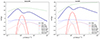 |
Fig. A.1. Density probabilities as a function of heliocentric relative proper motion for Gaia18ajz event for two mass functions, StellarIMF and DarkIMF, and their components from disk and bulge. Thin dashed lines show the density of lenses along the line of sight (distance prior), while dotted lines show the velocity (relative proper motion) priors. Dot-dashed line shows the mass function combined with the Jacobian. |
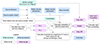 |
Fig. A.2. Schematic representation of steps done while estimating mass and distance of the lens with DarkLensCode. ML and DL are lens mass and distance respectively, mlens is lens’s observed magnitude, and mMS is the observed magnitude of a MS star of ML mass at a DL distance. |
Appendix B: Corner plots
The corner plots for the GO+ and GO- solutions are presented in Figures B.1 and B.2. These plots were generated using the corner Python package developed by Foreman-Mackey (2016).
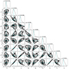 |
Fig. B.1. Corner plot of the microlensing parameters from the MCMC fit of the GO+ solution. The plot exhibits 1σ, 2σ, and 3σ confidence regions with solid black, dark grey, and light grey colors, respectively. Any solutions outside of the 3σ confidence level are represented by black dots. |
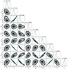 |
Fig. B.2. Corner plot of the microlensing parameters from the MCMC fit of the GO- solution. The plot exhibits 1σ, 2σ, and 3σ confidence regions with solid black, dark grey, and light grey colors, respectively. Any solutions outside of the 3σ confidence level are represented by black dots. |
All Tables
Optimal parameter values for fitting Gaia18ajz using only Gaia photometric data.
Optimal parameter values for fitting Gaia18ajz using both Gaia and ground-based follow-up photometric data.
Optimal parameter values for fitting Gaia18ajz, using Gaia and OGLE photometric data.
Equal-weight sample ratios of the solution with positive impact parameter to the solution with negative impact parameter u0.
Parameters of the source star determined via synthetic spectrum fitting and template matching.
DarkLensCode output for the GO- solution for each possible scenario. Estimations for the lens distance and mass, as well as θE, and the probability of the lens being a dark remnant for each possible scenario.
DarkLensCode output for the GO+ solution for each possible scenario. Estimations of the lens distance and mass, as well as θE, and the probability of the lens being a dark remnant.
All Figures
|
Fig. 1. Location of Gaia18ajz and its neighbourhood during the event. The image comes from Pan-STARRS DR1 via the Aladin Tool implemented in BHTOM. |
| In the text | |
|
Fig. 2. Photometric data collected for Gaia18ajz. The different colours represent different bands. |
| In the text | |
|
Fig. 3. Light curve of the Gaia18azj event and the microlensing model fit using only the Gaia data. The dashed magenta line represents the model without parallax, while the blue and black solid lines show the positive and negative solutions for the parallax model, respectively. The bottom panel shows the residuals with respect to the negative solution for the parallax model. |
| In the text | |
|
Fig. 4. Light curve of the Gaia18azj event and the microlensing model fit using the Gaia data as well as the ground-based survey data from ZTF, SMARTS, and OGLE. The dashed magenta line represents the model without parallax, while the blue and black solid lines show the positive and negative solutions for the parallax model, respectively. The bottom panel shows the residuals with respect to the negative solution for the parallax model. |
| In the text | |
|
Fig. 5. Light curve of the Gaia18azj event and the microlensing model fit using the Gaia data as well as the ground-based data from OGLE. The dashed magenta line represents the model without parallax, while the blue and black solid lines show the positive and negative solutions for the parallax model, respectively. The bottom panel shows the residuals with respect to the negative solution for the parallax model. |
| In the text | |
|
Fig. 6. Result of the synthetic spectrum fitting (red spectra) to the X-shooter spectroscopic data (blue spectra) generated for the best-matching atmospheric parameters. The Ca II triplet region is presented for two spectra obtained in 2018, March 25 (top panel) and August 8 (bottom panel) by using X-shooter. |
| In the text | |
|
Fig. 7. Two spectra from VLT/X-shooter obtained in March 25 (red) and August 8 (blue), 2018, as well as the best models with (solid lines) and without (dashed lines) extinction correction. The grey vertical lines and regions indicate the telluric bands, where the data were not used for the modelling. |
| In the text | |
|
Fig. 8. (Left) PARSEC stellar isochrones for 1.3, 2.2, 4.0, 7.1, and 12.6 Gyr with a fixed metallicity of −0.5. The source is most likely an old bright giant or supergiant. (Right) Source distance distribution based on PARSEC isochrones and the extinction estimated from the spectral modelling. Black dashed and dotted lines indicate the median distance value and the 1σ confident region, respectively. |
| In the text | |
|
Fig. 9. DarkLensCode output for the GO+ microlensing model assuming the DarkIMF. This diagram shows the posterior distribution of the distance to the lens and its mass. The colours correspond to the log probability density. The dark color of a bin means that there were no samples present in this bin. |
| In the text | |
|
Fig. 10. DarkLensCode output for the GO+ microlensing model assuming the StellarIMF mass function. Posterior distribution of the blended light magnitude and lens light magnitude assuming that the lens is an MS star. The solid line represents the upper limit of extinction, while the dashed line represents the lower limit of extinction. Lines separate the dark lens solutions from the MS star solutions. The colours correspond to the log probability density. Black bins are those containing no samples. |
| In the text | |
|
Fig. 11. Location of all parallax solutions for Gaia18ajz photometry superimposed on the distribution of tE and πE parameters expected for microlensing events using the simulated data from Kaczmarek et al. (2024). |
| In the text | |
|
Fig. A.1. Density probabilities as a function of heliocentric relative proper motion for Gaia18ajz event for two mass functions, StellarIMF and DarkIMF, and their components from disk and bulge. Thin dashed lines show the density of lenses along the line of sight (distance prior), while dotted lines show the velocity (relative proper motion) priors. Dot-dashed line shows the mass function combined with the Jacobian. |
| In the text | |
|
Fig. A.2. Schematic representation of steps done while estimating mass and distance of the lens with DarkLensCode. ML and DL are lens mass and distance respectively, mlens is lens’s observed magnitude, and mMS is the observed magnitude of a MS star of ML mass at a DL distance. |
| In the text | |
|
Fig. B.1. Corner plot of the microlensing parameters from the MCMC fit of the GO+ solution. The plot exhibits 1σ, 2σ, and 3σ confidence regions with solid black, dark grey, and light grey colors, respectively. Any solutions outside of the 3σ confidence level are represented by black dots. |
| In the text | |
|
Fig. B.2. Corner plot of the microlensing parameters from the MCMC fit of the GO- solution. The plot exhibits 1σ, 2σ, and 3σ confidence regions with solid black, dark grey, and light grey colors, respectively. Any solutions outside of the 3σ confidence level are represented by black dots. |
| In the text | |
Current usage metrics show cumulative count of Article Views (full-text article views including HTML views, PDF and ePub downloads, according to the available data) and Abstracts Views on Vision4Press platform.
Data correspond to usage on the plateform after 2015. The current usage metrics is available 48-96 hours after online publication and is updated daily on week days.
Initial download of the metrics may take a while.