| Issue |
A&A
Volume 692, December 2024
|
|
|---|---|---|
| Article Number | A28 | |
| Number of page(s) | 13 | |
| Section | Stellar structure and evolution | |
| DOI | https://doi.org/10.1051/0004-6361/202449322 | |
| Published online | 29 November 2024 | |
Dark lens candidates from Gaia Data Release 3
1
Astronomical Observatory, University of Warsaw, Al. Ujazdowskie 4, 00-478 Warszawa, Poland
2
Las Cumbres Observatory, 6740 Cortona Drive, Suite 102, Goleta, CA 93117, USA
3
Department of Particle Physics and Astrophysics, Weizmann Institute of Science, Rehovot 76100, Israel
4
Research School of Astronomy and Astrophysics, Australian National University, Mount Stromlo Observatory, Cotter Road, Weston Creek, ACT 2611, Australia
5
Zentrum für Astronomie der Universität Heidelberg, Astronomisches Rechen-Institut, Mönchhofstr. 12-14, 69120 Heidelberg, Germany
6
Institute of Theoretical Physics and Astronomy, Vilnius University, Saulėtekio al. 3, Vilnius LT-10257, Lithuania
7
Center for Astrophysics and Cosmology, University of Nova Gorica, Vipavska 11c, SI-5270 Ajdovščina, Slovenia
8
Department of Physics, University of Warwick, Gibbet Hill Road, Coventry CV4 7AL, UK
9
Institute for Space-Earth Environmental Research, Nagoya University, Nagoya 464-8601, Japan
10
Department of Earth and Space Science, Graduate School of Science, Osaka University, Toyonaka, Osaka 560-0043, Japan
11
Code 667, NASA Goddard Space Flight Center, Greenbelt, MD 20771, USA
12
Department of Astronomy, University of Maryland, College Park, MD 20742, USA
13
Institute of Natural and Mathematical Sciences, Massey University, Auckland 0745, New Zealand
14
Department of Earth and Planetary Science, Graduate School of Science, The University of Tokyo, 7-3-1 Hongo, Bunkyo-ku, Tokyo 113-0033, Japan
15
Institute of Astronomy, Graduate School of Science, The University of Tokyo, 2-21-1 Osawa, Mitaka, Tokyo 181-0015, Japan
16
Oak Ridge Associated Universities, Oak Ridge, TN 37830, USA
17
Institute of Space and Astronautical Science, Japan Aerospace Exploration Agency, 3-1-1 Yoshinodai, Chuo, Sagamihara, Kanagawa 252-5210, Japan
18
Sorbonne Université, CNRS, UMR 7095, Institut d’Astrophysique de Paris, 98 bis bd Arago, 75014 Paris, France
19
Department of Physics, University of Auckland, Private Bag 92019, Auckland, New Zealand
20
University of Canterbury Mt. John Observatory, P.O. Box 56 Lake Tekapo 8770, New Zealand
⋆ Corresponding author; kkruszynska@lco.global
Received:
23
January
2024
Accepted:
12
September
2024
Abstract
Gravitational microlensing is a phenomenon that allows us to observe the dark remnants of stellar evolution, even if these bodies are no longer emitting electromagnetic radiation. In particular, it can be useful to observe solitary neutron stars or stellar-mass black holes, providing a unique window through which to understand stellar evolution. Obtaining direct mass measurements with this technique requires precise observations of both the change in brightness and the position of the microlensed star. The European Space Agency’s Gaia satellite can provide both. Using publicly available data from different surveys, we analysed events published in the Gaia Data Release 3 (Gaia DR3) microlensing catalogue. Here, we describe our selection of candidate dark lenses, where we suspect the lens is a white dwarf (WD), a neutron star (NS), a black hole (BH), or a mass-gap object, with a mass in the range between the heaviest NS and the least massive BH. We estimated the mass of the lenses using information obtained from the best-fitting microlensing models, source star, Galactic model, and the expected parameter distributions. We found eleven candidates for dark remnants: one WDs, three NSs, three mass-gap objects, and four BHs.
Key words: gravitational lensing: micro / techniques: photometric / stars: black holes / stars: neutron / white dwarfs
© The Authors 2024
 Open Access article, published by EDP Sciences, under the terms of the Creative Commons Attribution License (https://creativecommons.org/licenses/by/4.0), which permits unrestricted use, distribution, and reproduction in any medium, provided the original work is properly cited.
This article is published in open access under the Subscribe to Open model. This email address is being protected from spambots. You need JavaScript enabled to view it. to support open access publication.
1. Introduction
Many outstanding questions related to the remnants of stellar evolution remain open. The most common stellar remnant is a white dwarf (WD) and more than 95% of stars will become a WD by the end of their lifetimes (Fontaine et al. 2001). Our understanding of white dwarfs was expanded in recent years by Gaia and its superb parallaxes. The largest such catalogue overall consists of over 350 000 high-confidence WD candidates, expanding almost tenfold the amount of known WDs before Gaia (Gentile Fusillo et al. 2021). The best catalogue of known pulsars is two orders of magnitude smaller than the one we have for WDs in our Galaxy (Manchester et al. 2005). The observational material available on BHs is the most limited, in particular solitary ones. Most of the known BHs are linked to binary systems found either through X-ray emission due to accretion of their companions (e.g. Corral-Santana et al. 2016) or as gravitational wave sources due to their merger (e.g. Abbott et al. 2019). Additionally, gravitational wave mergers are most frequently detected in distant galaxies. Recently, Shenar et al. (2022), El-Badry et al. (2023b), and El-Badry et al. (2023a), Chakrabarti et al. (2023) have reported on BH candidates also detected as non-interacting binary systems. However, the only known direct mass measurement for a solitary stellar-mass BH was recently presented for OGLE-2011-BLG-0462/MOA-2011-BLG-191 (Lam et al. 2022; Sahu et al. 2022; Mróz et al. 2022; Lam & Lu 2023) using the gravitational microlensing phenomenon.
Gravitational microlensing is an effect of Einstein’s general relativity, which occurs when a massive object passes in front of a distant star within the Milky Way or its neighbourhood (Einstein 1936; Paczynski 1986). In contrast to strong gravitational lensing, here the separated, deformed images of the source are typically impossible to spatially resolve unless the world’s largest telescopes are used, and only in case of very bright events (Dong et al. 2019; Cassan et al. 2022). Instead, what can be observed is a brightening of the source occurring during the event. Images of the source, though difficult to resolve, are unequally magnified and change position. This causes a distinctive shift in the centroid of light called astrometric microlensing (Dominik & Sahu 2000; Belokurov & Evans 2002). This effect can be measured with precise enough instruments such Hubble Space Telescope (HST; Sahu et al. 2017) or Gaia1.
Combining both effects allows the mass of the lens, ML, to be measured following Gould (2000):
 (1)
(1)
where κ = 4G/c2au ≈ 8.144mas/M⊙, θE is the angular Einstein Radius, which can be measured with astrometric microlensing, and πE is the microlensing parallax obtained from modelling the time-series photometry. A combination of these two effects was used to detect a stellar-mass BH for the first time in Lam et al. (2022) and Sahu et al. (2022), who used astrometric observations from HST and photometric observations from the ground.
However, even without a measurement of the angular Einstein radius, we can still estimate the mass of the lens by employing the Galactic model and expected distributions of lens parameters. We can obtain a posterior distribution for the lens mass and distance using the microlensing parallax, proper motion measurements, estimated distance to the source, the Galactic model and assumed mass function of stellar remnants (e.g. Wyrzykowski et al. 2016; Mróz & Wyrzykowski 2021). This method was used for objects observed by the OGLE survey where no Einstein radius information was available, where events exhibited clear parallax signal (e.g. Wyrzykowski & Mandel 2020; Mróz et al. 2021). The same technique could also be applied for microlensing events seen by Gaia (Prusti 2016), using both archival data and transients detected as part of Gaia Science Alerts (GSA) system (Hodgkin et al. 2021). This paper presents a similar analysis of Gaia Data Release 3 (Gaia DR3) microlensing catalogue (Wyrzykowski et al. 2023).
This work is split into six sections. Section 2 presents the microlensing models compared in this work, the criteria of event pre-selection and the sources of data used for this analysis. Section 3 explains the criteria to select events for detailed analysis, while Sect. 4 summarises those results. Section 6 shows how we estimated the masses and distances to the lenses. Section 7 discusses the obtained results and summarises this work.
2. Event pre-selection and data
2.1. Compared models
In this paper, we focused only on events that could exhibit the microlensing parallax effect, which occurs when the observer changes position during the event. There are three types of microlensing parallax: annual, terrestrial, and spatial. The annual microlensing parallax is connected to the Earth’s movement around the Sun. The observer on Earth changes their position during the entire year, which creates distinctive asymmetry and, in some cases, wobbles in the light curve (Gould 1992; Alcock et al. 1995; Maskoliūnas et al. 2023). The terrestrial parallax is connected to the different positions of the observatories on Earth. It is measurable only in the most extreme cases, such as catching a caustic crossing with telescopes on two sites distant from each other (Hardy & Walker 1995; Holz & Wald 1996; Gould et al. 2009). Finally, space parallax occurs when the event is observed from observatories located on Earth and in space. When the space observatory is located as far as one au from the Earth, it can cause a significant difference in the amplification and time of the peak of the lens (Refsdal 1966; Specht et al. 2023). We can be also measure whether the space observatory is closer but during a caustic crossing (Wyrzykowski et al. 2020) or if the event is densely covered. This is the main mechanism behind the way that the Nancy Grace Roman Space Telescope is going to be used for mass measurements of the observed lenses (Penny et al. 2019).
Gaia DR3 microlensing events catalogue contains events which were most likely caused by a single object as an outcome of the used pipeline (Wyrzykowski et al. 2023). All of the events within this catalogue were detected in the Galactic plane, which is a dense field, especially within the Galactic bulge. This means that we had to include blending when some of the light is coming from the stars near the line of sight towards the source and lens. In the case of microlensing, blending also factors in that the lens is luminous in the majority of cases.
We used the following models in our analysis with these parameters:
-
Point source-point lens (PSPL) model without blending, parameterised by t0, u0, tE, I0;
-
PSPL with blending, parameterised by t0, u0, tE, I0, fb;
-
PSPL model with parallax effect without blending, parameterised by t0, u0, tE, I0, πEN, πEE;
-
PSPL model with a parallax effect with blending, parameterised by t0, u0, tE, πEN, πEE, I0, fb;
where t0 is the time of the peak of brightness, u0 is the impact parameter at t0, and tE is the Einstein timescale when the source is crossing the angular Einstein ring. Microlensing parallax is described by its northern and eastern components πEN and πEE. The baseline magnitude of the event is denoted by I0 and the blending parameter is defined as  , where Fs is the source flux and Fb is the blend flux.
In this work, we used models without blending in the pre-selection stage, and for each event, we fit models with and without parallax. We used models with blending when we fitted each event individually. At this stage, we also fitted models with and without parallax. Each event should have at least two best-fitting solutions: PSPL without blending and PSPL with parallax and without blending.
2.2. Pre-selection of the candidate events
The Gaia Data Release 3, or alternatively table vari_microlensing of the Gaia DR3, contains 363 candidate events. Many of them do not exhibit second-order effects and are best described by the standard Paczyński model. We suspected that events with short Einsten timescales are less likely to be affected by the annual movement of the Earth around the Sun. Thus, we selected events with paczynski_0_te timescale longer than 50 days. This was an arbitrary cut, based on the fact that Gaia produces on average one point per month per source. An event with an Einstein timescale of 50 days would last more than 100 days, allowing for at least three observations during the event. Additionally, previous studies of candidate parallax events show that in most cases parallax is not detectable for shorter events (see for example Rodriguez et al. 2022 and Zhai et al. 2023). After applying this cut, we were left with 204 candidate events to analyse.
2.3. Data
The Wyrzykowski et al. (2023) catalogue was built using only GaiaG, GBP and GRP photometry; however, for the purposes of this work, we utilised data available from other surveys. In particular, we wanted to include information from microlensing surveys which have better cadence, especially in the Galactic bulge. We cross-matched the Gaia sources with the OGLE survey (Udalski et al. 1992, 2015). We found 145 events in common with the public OGLE events. Of these, 130 events were published as a part of the OGLE-IV analysis of microlensing optical depth in the Galactic plane (Mróz et al. 2019, 2020). 78 events were published were also published as OGLE Early Warning System alerts (Udalski et al. 2015)2, overlapping with the 130 events coming from the OGLE-IV papers. We downloaded all publicly available data. If the event was published in OGLE-EWS, Mróz et al. (2019) or Mróz et al. (2020), we used the data shared with the article. We performed a similar search with MOA survey (Abe et al. 1997; Bond et al. 2001) using its alert stream and we found 20 events in common. We found 32 events in common with KMTNet survey public alerts (Lee et al. 2014; Kim et al. 2016)3. Six events were published by Gaia Science Alerts4. These events were published with preliminary photometry and without errors. We simulated the errors using the following formula, (Wyrzykowski et al. 2023):
 (2)
(2)
where Gi is the i-th point in the GSA light curve. Since the error bars and photometric data had different properties, they came from different pipelines and the GSA data was created using raw photometric data. Gaia DR3 light curves were created by the photometric pipeline that was used on all data used for this Data Release and produced the most accurate light curves we have. We decided to treat them as a different dataset. Seven events were found in the publicly available data of the ASAS-SN survey (Shappee et al. 2014). Two were published as alerts: ASASSN-16li and ASASSN-16oe (Strader et al. 2016; Munari et al. 2016), and one was published as an ATEL (Jayasinghe et al. 2017). The rest was found in the ASAS-SN Photometric Database (Jayasinghe et al. 2019). We did not include Zwicky Transient Facility (ZTF; Bellm et al. 2019) while cross-matching events, because this survey started after May 2017, which was the end of Gaia DR3 timespan. We did, however, check for sources appearing in the 9th Data Release of ZTF if a given source brightened only once. The list of all 204 sources with their names in other surveys is available in Table A.1.
In the case of MOA and KMTNet, we used the available photometry published in fluxes, instead of magnitudes. KTMNet is a network of three robotic telescopes, located in Australia, South Africa, and Chile. These sites have different weather conditions, and when we used KMTNet DIA photometry, we separated each light curve by the observatory. For Gaia photometry, we followed Wyrzykowski et al. (2023), and modified the available uncertainties to match the method used to find candidate events.
All the data sources listed above were then used either at the preliminary or the detailed event modelling stages or both. We provide data used for this stage in a machine-readable online archive5.
3. Selection of candidate events for further analysis
To find preliminary models, we used the MulensModel package Poleski & Yee (2019) to generate microlensing models and the pyMultiNest package (Feroz et al. 2009; Buchner et al. 2014) to find the best fitting solutions. To simplify the parameter space explored by the pyMultiNest package, we calculated models without blending. pyMultiNest provides a Python interface for a nested sampling algorithm which returns the best solutions for probability densities containing multiple modes and degeneracies. This made it a perfect tool for comparing models including microlensing parallax. For the parallax model, we included both the annual and space effects. Gaia is located in space and there may be an offset between observatories.
We have recorded the four best solutions for models with and without parallax and compared their χ2 values. These solutions are available in machine-readable format. Using preliminary models, we selected events, that:
-
had Einstein timescale of the best PSPL solution larger than 50 days, and
-
the difference of χ2 per degrees-of-freedom of the best PSPL model and the best parallax model should be larger than one (χPSPL2/d.o.f. − χPar2/d.o.f. > 1).
This way we selected 34 events. We removed two events from this sample. For the first one (GaiaDR3-ULENS-024), we did not have a full light curve and the event did not finish before the end of the Gaia DR3 period. The second one (GaiaDR3-ULENS-178) turned out to be a binary event, when we inspected the MOA light curve. We decided to add three additional events, which had ASAS-SN data (GaiaDR3-ULENS-023, GaiaDR3-ULENS-032, and GaiaDR3-ULENS-118). In these cases, the automatic algorithm struggled to find a correct solution and we concluded that was caused by the vastly different pixel size of the ASAS-SN, compared to Gaia and other surveys, as well as the exclusion of blending in fitted models.
4. Detailed analysis of selected events
We conducted a case-by-case analysis of the 35 events selected in the previous step. We used MulensModel to generate the microlensing models and emcee (Foreman-Mackey et al. 2013) to explore the parameter space. In this step, we used the KMTNet pySIS photometric data in magnitudes. For KMTNet data, when possible, we pre-processed data, removing any points that had a negative value of FWHM column or with a photometric uncertainty greater than one magnitude. For OGLE and MOA events, we used re-processed data coming from the end-of-the-season DIA photometric reduction pipelines (Udalski et al. 2015; Bond et al. 2001). We also applied a correction procedure for uncertainties following Skowron et al. (2016) to OGLE data from bulge fields. Finally, we re-scaled the photometric uncertainties using this formula:
 (3)
(3)
where σ′n, i is the re-scaled i-th uncertainty of the n-th telescope’s light curve, kn is the scale factor for the n-th telescope, and σn, i is the original i-th uncertainty of the n-th telescope’s light curve. We obtained the scale factors in the following manner:
-
First, fitting the preliminary PSPL models with and without parallax;
-
Then selecting a model with the smallest χ2 value;
-
Finally, using this model we used it as a starting point, we ran an MCMC fit with scale factors as one of the fit parameters.
If the scale factor of the median solution found in the final step exceeded 1.0 for a given telescope, we used this value and then we re-fit the PSPL models with and without parallax. For events GaiaDR3-ULENS-003, GaiaDR3-ULENS-032, GaiaDR3-ULENS-118, GaiaDR3-ULENS-196, and GaiaDR3-ULENS-284. we had to use the PSPL without a parallax model – instead of the best model to find the scale factors. For event GaiaDR3-ULENS-025, GaiaDR3-ULENS-143, we could not find scale factors due to poor event coverage. We report the values for each scale factor in Appendix A.2. For some events, we had to perform an outlier removal procedure. We did this before applying the uncertainty re-scaling. We used the best-fitting preliminary model (step 2 of the uncertainty re-scaling procedure). Then we removed all data points outside the 3 σ range of the residuals from the preliminary model for a given light curve. We marked those light curves in bold in Table A.2. In some cases, we had to remove certain light curves, because they were too noisy or carried little information about the event. We marked those datasets with a strike-through text in Table A.2. Table A.2 provides the name of the fitted event and a list of datasets with the amount of data points for each light curve. Table A.4 presents the median values of the posterior distributions (PDFs) obtained for the best-fitting solutions. The KMTNet data for event GaiaDR3-ULENS-047/KMT-2015-BLG-0157 revealed features around the peak, for which a PSPL model was not able to characterise, so it was excluded from further analysis. GaiaDR3-ULENS-284 had a large parallax value, which means other effects should be included. We excluded that event from further analysis. GaiaDR3-ULENS-057 had only three points at magnification, so we could only find a non-parallax solution. We named the solutions with the following convention, “Gaia DR3-AAA-BC”, where AAA is the number assigned to the event in Wyrzykowski et al. (2023), B is a string of letters denoting which type of Gaia data was used, “G” for events where we used the Gaia DR3 photometry, and “GSA” for events where we opted for a Gaia Science Alerts light curve, finally C is a sign of the u0 of the solution (“+” for positive and “–” for negative). If there was more than one solution with the same u0 sign, we numbered them starting from 1.
To select the dark lens candidate sample, we applied the following criteria to the modelled events:
-
the blending parameter in G band was smaller than 0.3;
-
the πEE was not consistent with zero in the three-sigma range;
-
the χ2 of the parallax solution was smaller than the χ2 of the non-parallax solution.
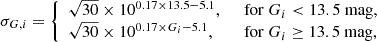
In this way, we obtained 14 events, where at least one solution passed those criteria. For these events, we then estimated the lens distance and mass. From the remaining events, a non-parallax model better described two of them, seven did not pass the blending parameter criterion, and six did not pass the πEE criterion. We found four events that passed the blending and χ2 criterion, but failed the πEE criterion in the calculated three sigma; however, their πEE distribution was inconsistent with 0. We analysed these solutions further, but display their results in a different table (Table A.6). An example of a light curve is shown in Figure 1.
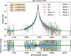 |
Fig. 1. Light curve of the event known as GaiaDR3-ULENS-343, BLG502.29.100629 Mróz et al. (2019), OGLE-2017-BLG-0095, MOA-2017-BLG-160, and KMT-2017-BLG-1123, shown at the top. The GaiaG data is shown in green, GRP in red, KMTNet data is shown in dark red, violet and aqua for the South African Astronomical Observatory (KMTA), Cerro Tololo Inter-American Observatory (KMTC), and Siding Springs Observatory (KMTS), MOA I and V band data are shown in light green and dark red respectively, and OGLE in light-blue. The four solutions are marked: PSPL without parallax G0 with a black dashed line, and two PSPLs with parallax, G+ and G- with red and grey continuous lines respectively. The bracket in the top left shows the χ2 of different solutions. Bottom panel: Residuals of the G+ model. A Black dashed line marks the G0 and G+ models difference, while the dark grey continuous line marks the G+ and G- models difference, respectively. |
5. Source stars
To determine the properties of the lens, we have to determine the properties of the source. Ideally, we would obtain the distance to the source, but this is not always possible. Instead, we decided to find the angular stellar radius of the source θ* and use it as a prior during lens mass and distance estimation. We followed different procedures, depending on the event location and available information.
We were able to use the colour-magnitude diagrams (CMDs) calibrated to the OGLE-III data for events with MOA data (GaiaDR3-ULENS-035, GaiaDR3-ULENS-069, GaiaDR3-ULENS-073, GaiaDR3-ULENS-088, GaiaDR3-ULENS-155, GaiaDR3-ULENS-343, and GaiaDR3-ULENS-353). First, we determined the red clump centre (RCG) location, following the procedure outlined in Nataf et al. (2013). We used the de-reddened RCG distance modulus determined in Nataf et al. (2013) for each event6 and found the reddened distance modulus of the RCG using fitted position on the CMD and absolute magnitude of the RCG MI, RCG = ( − 0.12, 1.06) mag Nataf et al. (2013), Bensby et al. (2013). Then we calculate the extinction in AI and AV and use it to find the de-reddened magnitude and colour of the source. In the case of GaiaDR3-ULENS-353, the blending parameter was negative; so instead of using the calculated source magnitude, we used the baseline magnitudes to determine the source brightness and colour. Finally, we used these values to determine the angular stellar radius of the source star using relations from Adams et al. (2018).
Other sources were more difficult. If the source was located towards the Galatic Bulge, we assumed that the Bulge is located 8.1 kpc and extends for 2.4 kpc. We used this value to determine the de-reddened distance modulus to the red clump centre. We constructed a CMD in V and I data using Gaia DR3 sources. We selected sources within 30’ of the event, that had the Renormalized Unit Weight Error (RUWE) parameter smaller than 1.4, astrometric parallax error not larger than 20% of the measured value, and that had available GSP-Phot solutions (Andrae et al. 2023). Then, we transformed their colours into V and I bands following relations from Busso et al. (2022) Sect. 5.5.17. We determined the position of the RGC following the procedure in Nataf et al. (2013), and used the calculated distance modulus to find the extinction in I and V bands. Finally, we found the θ* using relation from Adams et al. (2018). We used this method for events GaiaDR3-ULENS-025, GaiaDR3-ULENS-089, GaiaDR3-ULENS-142, and GaiaDR3-ULENS-270. For many of these events, some information was missing. When baseline magnitude and blending in GBP and/or GRP filter, we used blending parameter in G (for GBP) or in I (for GRP) bands and Gaia DR3 entry for this source to determine the missing brightness for the θ* estimation. We could not use this method for events GaiaDR3-ULENS-331 and GaiaDR3-ULENS-363, because they were too dim compared to the data with GSP-Phot entries to infer the extinction.
Finally, for events located towards the Galactic disc, we were not able to determine the de-reddened distance modulus towards the RCG, and therefore θ*. This affected events GaiaDR3-ULENS-103, GaiaDR3-ULENS-118, and GaiaDR3-ULENS-259. All the determined values can be found in Table A.3. An example of a CMD is shown in Figure 2.
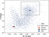 |
Fig. 2. Colour-magnitude diagram based using MOA data calibrated to OGLE-III catalogue for event GaiaDR3-ULENS-343. MOA data is displayed in light blue dots. The red dot marks the source position, black dot marks the blended baseline source colour and magnitude. Dashed lines mark the region that we used for estimating RGC, and the dark blue star represents the found RGC position. |
6. Estimating the lens parameters of candidate dark events
We used the same approach presented in Wyrzykowski et al. (2016), Mróz & Wyrzykowski (2021), and Kruszyńska et al. (2022) to estimate the mass and distance to the lens. We dubbed it the DarkLensCode8 and we explain this method in greater detail in Howil et al. (2024). The DarkLensCode was used to find the posterior distribution of lens distance and lens mass, using the PDFs of the photometric model parameters and the Galactic model. The final estimates are the median values of obtained mass and distance PDFs. Here, we focus on the presentation and the resulting mass and distance estimates. We present the results in Tables A.5 and A.6.
If we found more than one solution passed the criteria outlined in Sect. 4, we analysed them separately, providing mass estimates for each solution. The extinction AG was calculated following a method similar to one outlined in Fukui et al. (2019), but we used Gaia DR3 data instead. We selected all sources within a 30’ radius with a renormalised unit weight error parameter smaller than 1.4, a parallax uncertainty smaller than 20% of the measured value, and the available GSP-Phot solutions (Andrae et al. 2023). Then, we calculated the mean and standard deviation of the ag_gspphot in 50 pc bins and fit a fourth-order polynomial. We used the fitted polynomial as a function of extinction depending on the distance towards the lens or the source. If the distance to the lens or source was larger than 8 kpc, we used the calculated extinction value AG at 8 kpc.
We did not know the distance to the source, so we assumed different maximum and minimum ranges. For events located towards the bulge, we initially assumed that the distance can be between 1 kpc and 12 kpc. For events located towards the disc, we chose the distance between 0.1 kpc and 8 kpc (GaiaDR3-ULENS-118) or 10 kpc (GaiaDR3-ULENS-259). When available, we used the value of θ* derived in Sect. 5. First, we randomly selected a distance to the source from the range described above and calculated the source radius RS. In the next step, we found the absolute magnitude of the source star. The procedure depended on the position of the source star in the CMD.
If the source star position on the CMD was located in the main sequence, we assumed the star was a dwarf. Using the tables from Pecaut & Mamajek (2013) provided on the author’s website9 we found the corresponding value of absolute magnitude in G band.
If the source star position on the CMD was located in the red giant clump, we assumed the star was a giant. For the absolute magnitude determination, we followed the information contained in van Belle et al. (2021). First, we found the (V0 − K0) value corresponding to the radius based on the inverted relation presented in the paper with coefficients coming from Table 16. Then we used Eq. (4) from van Belle et al. (2021) to find the effective temperature Teff of the source star. We used the well-known relation Lbol = 4πRS2σSBTeff4 to find the bolometric luminosity of the source star. To find the bolometric correction BCG in G band, we followed the recipe provided in Manteiga et al. (2018), Chapter 8.3.3. Finally, we were able to derive the absolute magnitude in G following Eq. (8.6) from Manteiga et al. (2018).
We then found the extinction, AG, and the observed magnitude of the source star at a selected distance. If the absolute value of the difference between the calculated source magnitude and the observed source magnitude from the microlensing model was smaller than the sum of the source magnitude uncertainty from the model and the derived source magnitude uncertainty, we accepted that source distance value.
We used three mass functions as lens mass priors with the Kroupa (2001) function that describes stars:
 (4)
(4)
then the Mróz et al. (2021) function that describes solitary dark remnants in our Galaxy:
 (5)
(5)
and a f(M)∼M−1 corresponding to applying no prior on the lens function. The reported values of the lens mass and distance are median values of the posterior distribution, while their uncertainty is represented by the 16th and 84th quantiles.
We noticed that the mass function greatly affects the lens mass estimate. Using the Kroupa (2001) mass function results in lighter lenses at greater distances, and in turn more likely MS stars. In contrast, the Mróz et al. (2021) mass function produced more massive lenses at closer distances. This is because the Kroupa (2001) mass function is steeper and less likely to produce massive lenses.
We compared the brightness of the blend from the microlensing model to the brightness of an MS star at an estimated distance from the lens. We summed the number of solutions where the brightness of the blend was smaller than the MS brightness and divided this number by the number of all solutions. The resulting number was interpreted as the probability that the lens is dark and not an MS star. All input parameters are available in machine-readable form in an online archive attached to this paper.
https://github.com/KKruszynska/dark_lens_plots/
7. Discussion and conclusions
We found a total of 11 lenses for which the probability for the dark lens scenario for at least one solution exceeded 80% when we looked only at the Kroupa (2001) mass function. Eight of them passed all of the criteria imported in Sect. 4 (GaiaDR3-ULENS-025, GaiaDR3-ULENS-035, GaiaDR3-ULENS-069, GaiaDR3-ULENS-073, GaiaDR3-ULENS-088, GaiaDR3-ULENS-155, GaiaDR3-ULENS-343, and GaiaDR3-ULENS-353). Among the solutions that did not pass the πEE criterion, we found three more candidates (GaiaDR3-ULENS-103, GaiaDR3-ULENS-212, GaiaDR3-ULENS-331, and GaiaDR3-ULENS-155, but we accounted for this event in the first group). All but one of these events have Galactic coordinates towards the Galactic centre. The estimated distance for 16 solutions (eight events) would suggest that they are located in the Galactic disc, rather than the Galactic bulge. For three solutions (two events), the estimated lens distance suggests a Galactic bulge lens. Three events seem to have the lens located within one kiloparsec from Earth. One event located towards the Galactic disc seems to have a lens no closer than 3.1 kpc, which means it would belong to the Scutum-Centaurus Arm of the Milky Way.
If we assumed that all of those 11 events are dark lenses, and instead follow a Mróz et al. (2021) mass function, we would end up with the majority of events with masses in the range of mass-gap objects and black holes. One event, GaiaDR3-ULENS-035, has mass consistent with a white dwarf, and three (GaiaDR3-ULENS-025, GaiaDR3-ULENS-155, and GaiaDR3-ULENS-212) are consistent with a neutron star. Three events, GaiaDR3-ULENS-069, GaiaDR3-ULENS-103, and GaiaDR3-ULENS-343 overlap with the first mass gap in the one-sigma range. Four objects have higher masses (GaiaDR3-ULENS-073, GaiaDR3-ULENS-088, GaiaDR3-ULENS-331, and GaiaDR3-ULENS-353) are consistent with BHs. All BH candidates have large uncertainties and there are issues with mass estimates for two of them. For GaiaDR3-ULENS-073, we struggled with finding the correct position of the RGC, which could result in the wrong source distance, leading to the wrong lens distance. Second, GaiaDR3-ULENS-331 belongs to the group that did not pass the πEE criterion in Sect. 4. We present these estimates here, along with a comparison to dark remnant mass estimates found through other methods in Fig. 3.
 |
Fig. 3. Distribution of known masses of WDs, NS and BHs. Light pink marks WDs known from Gaia (Gentile Fusillo et al. 2021). In light red we marked NS with known masses coming from John Antoniadis’s catalogue (Lattimer 2012; Antoniadis 2013). Objects found by gravitational wave detectors were marked in yellow (Abbott et al. 2019, 2021a, 2024, 2023, 2021b). In red we marked high mass x-ray binaries (Orosz et al. 2007; Val-Baker et al. 2007; Orosz et al. 2009, 2014; Corral-Santana et al. 2016; Miller-Jones et al. 2021). In light blue, we marked candidates for dark remnants found by microlensing (Sahu et al. 2017; Kaczmarek et al. 2022; Kruszyńska et al. 2022; Jabłońska et al. 2022; McGill et al. 2023), including Lam & Lu (2023). In olive, we marked non-interacting dark remnants (Shenar et al. 2022; El-Badry et al. 2023b,a; Chakrabarti et al. 2023; El-Badry et al. 2024; Panuzzo 2024). Black dots mark masses of objects known from this work. Each solution for the event is shown separately. We marked solutions with positive u0 with circles, and negative with diamonds. Dashed, vertical lines mark different mass thresholds: the left-most is the Chandrasekhar mass limit, second to the left is the Tolman-Volkoff-Oppenheimer limit, and two right-most mark the limits for the theoretical pair-instability supernovae region (Farmer et al. 2020). A solid vertical line marks the conventional limit of 5 M⊙ for the lightest BHs. Data used to create this plot can be found in a GitHub repository. |
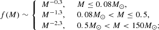
In the case of events where Gaia reported a proper motion, we calculated the transverse velocity. We present results for selected nine events in Fig. 4. There is one high-velocity events: GaiaDR3-ULENS-212. This event has a relatively short Einstein timescale of 56 days. The estimated mass is consistent with an NS. The proper motion found in Gaia DR3 is not out of the ordinary, so this means that the lens would have to move fast to justify the relative proper motion and the resulting Einstein timescale.
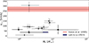 |
Fig. 4. Transverse velocities, vt, L, estimated for nine candidate events using DarkLensCode and Gaia proper motion measurements. ML is the mass of the lens. Black dots represent estimates of the masses and velocities of the nine candidates with error bars as lines, and each solution is plotted separately. We marked solutions with positive u0 with circles and negative ones with diamonds. The red line represents the median transverse velocity of NS from Hobbs et al. (2005), with a light red rectangle representing their dispersion. The dark blue rectangle represents the mass and transverse velocity of the BH from Lam & Lu (2023). |
All nine objects seem to separate into two groups: high velocity, similar to the NS velocity from Hobbs et al. (2005), and low velocity, similar to the velocity of a solitary BH from Lam & Lu (2023). The velocity does not seem to depend on the lens mass, but the error bars are large and it is hard to draw conclusive statements. Moreover, here we are most likely getting an estimate of a velocity coming from a Galactic prior. More accurate estimates will be possible once we obtain an astrometric time series for these events.
Here, we also measure only the most likely mass of candidate events. We cannot, however, confirm their nature as WDs, NS or BHs until we perform additional observations in other ranges of electromagnetic radiation, especially in the X-ray and UV. They could be some unusual objects, such as quark stars, or products of primordial black hole (PBH) mergers with other objects. Abramowicz et al. (2018) and Abramowicz et al. (2022) revealed a mechanism that could produce a low-mass BH from a moon-mass PBH (1025 g > MPBH > 1017 g) collision with an NS. Such low-mass BH would be in the mass range of an NS.
It is worth noting that these are only candidates for dark lenses and their mass measurement will be possible only when we will include astrometric time series. This data will be available only with Gaia DR4, no sooner than the end of 2025. This is an exciting prospect, as Gaia may allow us to observe previously unseen stellar populations. This becomes even more promising with the approaching start of the Vera C. Rubin Observatory and its Legacy Survey of Space and Time (Ivezić et al. 2019), as well as the launch of the Roman mission (Spergel et al. 2015; Akeson et al. 2019). Rubin will allow us to select long-duration microlensing events from the entire Galactic plane, whereas Roman is equipped to provide high-cadence astrometric and photometric observations in the Galactic bulge.
Data availability
Full Tables A.1–A.4 are available at the CDS via anonymous ftp to cdsarc.cds.unistra.fr (130.79.128.5) or via https://cdsarc.cds.unistra.fr/viz-bin/cat/J/A+A/692/A28
Acknowledgments
KK would like to thank Monika Sitek, Drs. Etienne Bachelet, Mariusz Gromadzki, Przemek Mróz, Radek Poleski, Milena Ratajczak, Rachel Street, Paweł Zieliński, Przemysław Mikołajczyk, as well as Profs. Michał Bejger, Wojciech Hellwing, Katarzyna Małek, and Łukasz Stawarz. This work was supported from the Polish NCN grants: Harmonia No. 2018/30/M/ST9/00311, Daina No. 2017/27/L/ST9/03221, and NCBiR grant within POWER program nr POWR.03.02.00-00-l001/16-00. LW acknowledges MNiSW grant DIR/WK/2018/12 and funding from the European Union’s Horizon 2020 research and innovation program under grant agreement No. 101004719 (OPTICON-RadioNET Pilot, ORP). The MOA project is supported by JSPS KAKENHI Grant Number JP24253004, JP26247023, JP16H06287 and JP22H00153. This work has made use of data from the European Space Agency (ESA) mission Gaia (https://www.cosmos.esa.int/gaia), processed by the Gaia Data Processing and Analysis Consortium (DPAC, https://www.cosmos.esa.int/web/gaia/dpac/consortium). Funding for the DPAC has been provided by national institutions, in particular, the institutions participating in the Gaia Multilateral Agreement. We acknowledge ESA Gaia, DPAC and the Photometric Science Alerts Team (http://gsaweb.ast.cam.ac.uk/alerts). This research has made use of publicly available data (https://kmtnet.kasi.re.kr/ulens/) from the KMTNet system operated by the Korea Astronomy and Space Science Institute (KASI) at three host sites of CTIO in Chile, SAAO in South Africa, and SSO in Australia. Data transfer from the host site to KASI was supported by the Korea Research Environment Open NETwork (KREONET).
References
- Abbott, B. P., Abbott, R., Abbott, T. D., et al. 2019, Phys. Rev. X, 9, 031040 [Google Scholar]
- Abbott, R., Abbott, T. D., Abraham, S., et al. 2021a, Phys. Rev. X, 11, 021053 [Google Scholar]
- Abbott, R., Abbott, T. D., Abraham, S., et al. 2021b, SoftwareX, 13, 100658 [NASA ADS] [CrossRef] [Google Scholar]
- Abbott, R., Abbott, T. D., Acernese, F., et al. 2023, Phys. Rev. X, 13, 041039 [Google Scholar]
- Abbott, R., Abbott, T. D., Acernese, F., et al. 2024, Phys. Rev. D, 109, 022001 [NASA ADS] [CrossRef] [Google Scholar]
- Abe, F., Allen, W., Banks, T., et al. 1997, Variables Stars and the Astrophysical Returns of the Microlensing Surveys (Gif-sur-Yvette, France: Editions Frontieres), 75 [Google Scholar]
- Abramowicz, M. A., Bejger, M., & Wielgus, M. 2018, ApJ, 868, 17 [NASA ADS] [CrossRef] [Google Scholar]
- Abramowicz, M., Bejger, M., Udalski, A., & Wielgus, M. 2022, ApJ, 935, L28 [NASA ADS] [CrossRef] [Google Scholar]
- Adams, A. D., Boyajian, T. S., & von Braun, K. 2018, MNRAS, 473, 3608 [NASA ADS] [CrossRef] [Google Scholar]
- Akeson, R., Armus, L., Bachelet, E., et al. 2019, arXiv e-prints [arXiv:1902.05569] [Google Scholar]
- Alcock, C., Allsman, R. A., Alves, D., et al. 1995, ApJ, 454, L125 [NASA ADS] [CrossRef] [Google Scholar]
- Andrae, R., Fouesneau, M., Sordo, R., et al. 2023, A&A, 674, A27 [CrossRef] [EDP Sciences] [Google Scholar]
- Antoniadis, J. I. 2013, PhD thesis, Rheinische Friedrich Wilhelms University of Bonn, Germany [Google Scholar]
- Bellm, E. C., Kulkarni, S. R., Graham, M. J., et al. 2019, PASP, 131, 018002 [Google Scholar]
- Belokurov, V. A., & Evans, N. W. 2002, MNRAS, 331, 649 [NASA ADS] [CrossRef] [Google Scholar]
- Bensby, T., Yee, J. C., Feltzing, S., et al. 2013, A&A, 549, A147 [NASA ADS] [CrossRef] [EDP Sciences] [Google Scholar]
- Bond, I. A., Abe, F., Dodd, R. J., et al. 2001, MNRAS, 327, 868 [Google Scholar]
- Buchner, J., Georgakakis, A., Nandra, K., et al. 2014, A&A, 564, A125 [NASA ADS] [CrossRef] [EDP Sciences] [Google Scholar]
- Busso, G., Cacciari, C., Bellazzini, M., et al. 2022, Gaia DR3 Documentation Chapter 5: Photometric Data, Gaia DR3 Documentation, European Space Agency; Gaia Data Processing and Analysis Consortium, 5 [Google Scholar]
- Cassan, A., Ranc, C., Absil, O., et al. 2022, Nat. Astron., 6, 121 [NASA ADS] [CrossRef] [Google Scholar]
- Chakrabarti, S., Simon, J. D., Craig, P. A., et al. 2023, AJ, 166, 6 [NASA ADS] [CrossRef] [Google Scholar]
- Corral-Santana, J. M., Casares, J., Muñoz-Darias, T., et al. 2016, A&A, 587, A61 [NASA ADS] [CrossRef] [EDP Sciences] [Google Scholar]
- Dominik, M., & Sahu, K. C. 2000, ApJ, 534, 213 [CrossRef] [Google Scholar]
- Dong, S., Mérand, A., Delplancke-Ströbele, F., et al. 2019, ApJ, 871, 70 [CrossRef] [Google Scholar]
- Einstein, A. 1936, Science, 84, 506 [NASA ADS] [CrossRef] [Google Scholar]
- El-Badry, K., Rix, H.-W., Cendes, Y., et al. 2023a, MNRAS, 521, 4323 [NASA ADS] [CrossRef] [Google Scholar]
- El-Badry, K., Rix, H.-W., Quataert, E., et al. 2023b, MNRAS, 518, 1057 [Google Scholar]
- El-Badry, K., Simon, J. D., Reggiani, H., et al. 2024, Open J. Astrophys., 7, 27 [NASA ADS] [Google Scholar]
- Farmer, R., Renzo, M., de Mink, S. E., Fishbach, M., & Justham, S. 2020, ApJ, 902, L36 [CrossRef] [Google Scholar]
- Feroz, F., Hobson, M. P., & Bridges, M. 2009, MNRAS, 398, 1601 [NASA ADS] [CrossRef] [Google Scholar]
- Fontaine, G., Brassard, P., & Bergeron, P. 2001, PASP, 113, 409 [NASA ADS] [CrossRef] [Google Scholar]
- Foreman-Mackey, D., Hogg, D. W., Lang, D., & Goodman, J. 2013, PASP, 125, 306 [Google Scholar]
- Fukui, A., Suzuki, D., Koshimoto, N., et al. 2019, AJ, 158, 206 [NASA ADS] [CrossRef] [Google Scholar]
- Gaia Collaboration (Prusti, T., et al.) 2016, A&A, 595, A1 [NASA ADS] [CrossRef] [EDP Sciences] [Google Scholar]
- Gaia Collaboration (Panuzzo, P., et al.) 2024, A&A, 686, L2 [NASA ADS] [CrossRef] [EDP Sciences] [Google Scholar]
- Gentile Fusillo, N. P., Tremblay, P. E., Cukanovaite, E., et al. 2021, MNRAS, 508, 3877 [NASA ADS] [CrossRef] [Google Scholar]
- Gould, A. 1992, ApJ, 392, 442 [Google Scholar]
- Gould, A. 2000, ApJ, 542, 785 [NASA ADS] [CrossRef] [Google Scholar]
- Gould, A., Udalski, A., Monard, B., et al. 2009, ApJ, 698, L147 [Google Scholar]
- Hardy, S. J., & Walker, M. A. 1995, MNRAS, 276, L79 [NASA ADS] [Google Scholar]
- Hobbs, G., Lorimer, D. R., Lyne, A. G., & Kramer, M. 2005, MNRAS, 360, 974 [Google Scholar]
- Hodgkin, S. T., Harrison, D. L., Breedt, E., et al. 2021, A&A, 652, A76 [NASA ADS] [CrossRef] [EDP Sciences] [Google Scholar]
- Holz, D. E., & Wald, R. M. 1996, ApJ, 471, 64 [NASA ADS] [CrossRef] [Google Scholar]
- Howil, K., Wyrzykowski, Ł., Kruszyńska, K., et al. 2024, arXiv e-prints [arXiv:2403.09006] [Google Scholar]
- Ivezić, Ž., Kahn, S. M., Tyson, J. A., et al. 2019, ApJ, 873, 111 [Google Scholar]
- Jabłońska, M., Wyrzykowski, Ł., Rybicki, K. A., et al. 2022, A&A, 666, L16 [NASA ADS] [CrossRef] [EDP Sciences] [Google Scholar]
- Jayasinghe, T., Kochanek, C. S., Stanek, K. Z., et al. 2017, ATel, 10677, 1 [NASA ADS] [Google Scholar]
- Jayasinghe, T., Stanek, K. Z., Kochanek, C. S., et al. 2019, MNRAS, 485, 961 [Google Scholar]
- Kaczmarek, Z., McGill, P., Evans, N. W., et al. 2022, MNRAS, 514, 4845 [CrossRef] [Google Scholar]
- Kim, S.-L., Lee, C.-U., Park, B.-G., et al. 2016, J. Korean Astron. Soc., 49, 37 [Google Scholar]
- Kroupa, P. 2001, MNRAS, 322, 231 [NASA ADS] [CrossRef] [Google Scholar]
- Kruszyńska, K., Wyrzykowski, Ł., Rybicki, K. A., et al. 2022, A&A, 662, A59 [NASA ADS] [CrossRef] [EDP Sciences] [Google Scholar]
- Lam, C. Y., & Lu, J. R. 2023, ApJ, 955, 116 [NASA ADS] [CrossRef] [Google Scholar]
- Lam, C. Y., Lu, J. R., Udalski, A., et al. 2022, ApJ, 933, L23 [NASA ADS] [CrossRef] [Google Scholar]
- Lattimer, J. M. 2012, Annu. Rev. Nucl. Part. Sci., 62, 485 [NASA ADS] [CrossRef] [Google Scholar]
- Lee, C.-U., Kim, S.-L., Cha, S.-M., et al. 2014, Proc. SPIE, 9145, 91453T [NASA ADS] [CrossRef] [Google Scholar]
- Manchester, R. N., Hobbs, G. B., Teoh, A., & Hobbs, M. 2005, AJ, 129, 1993 [Google Scholar]
- Manteiga, M., Andrae, R., Fouesneau, M., et al. 2018, Gaia DR2 Documentation Chapter 8: Astrophysical Parameters, Gaia DR2 documentation, European Space Agency; Gaia Data Processing and Analysis Consortium, 8 [Google Scholar]
- Maskoliūnas, M., Wyrzykowski, Ł, Howil, K., et al. 2023, A&A submitted [arXiv:2309.03324] [Google Scholar]
- McGill, P., Anderson, J., Casertano, S., et al. 2023, MNRAS, 520, 259 [NASA ADS] [CrossRef] [Google Scholar]
- Miller-Jones, J. C. A., Bahramian, A., Orosz, J. A., et al. 2021, Science, 371, 1046 [Google Scholar]
- Mróz, P., & Wyrzykowski, Ł. 2021, Astron. Comput., 71, 89 [Google Scholar]
- Mróz, P., Udalski, A., Skowron, J., et al. 2019, ApJS, 244, 29 [Google Scholar]
- Mróz, P., Udalski, A., Szymański, M. K., et al. 2020, ApJS, 249, 16 [CrossRef] [Google Scholar]
- Mróz, P., Udalski, A., Wyrzykowski, L., et al. 2021, arXiv e-prints [arXiv:2107.13697] [Google Scholar]
- Mróz, P., Udalski, A., & Gould, A. 2022, ApJ, 937, L24 [CrossRef] [Google Scholar]
- Munari, U., Hambsch, F. J., & Frigo, A. 2016, ATel, 9879, 1 [NASA ADS] [Google Scholar]
- Nataf, D. M., Gould, A., Fouqué, P., et al. 2013, ApJ, 769, 88 [Google Scholar]
- Orosz, J. A., McClintock, J. E., Narayan, R., et al. 2007, Nature, 449, 872 [NASA ADS] [CrossRef] [Google Scholar]
- Orosz, J. A., Steeghs, D., McClintock, J. E., et al. 2009, ApJ, 697, 573 [NASA ADS] [CrossRef] [Google Scholar]
- Orosz, J. A., Steiner, J. F., McClintock, J. E., et al. 2014, ApJ, 794, 154 [NASA ADS] [CrossRef] [Google Scholar]
- Paczynski, B. 1986, ApJ, 304, 1 [NASA ADS] [CrossRef] [Google Scholar]
- Pecaut, M. J., & Mamajek, E. E. 2013, ApJS, 208, 9 [Google Scholar]
- Penny, M. T., Gaudi, B. S., Kerins, E., et al. 2019, ApJS, 241, 3 [CrossRef] [Google Scholar]
- Poleski, R., & Yee, J. C. 2019, Astronomy and Computing, 26, 35 [NASA ADS] [CrossRef] [Google Scholar]
- Refsdal, S. 1966, MNRAS, 134, 315 [NASA ADS] [CrossRef] [Google Scholar]
- Rodriguez, A. C., Mróz, P., Kulkarni, S. R., et al. 2022, ApJ, 927, 150 [Google Scholar]
- Sahu, K. C., Anderson, J., Casertano, S., et al. 2017, Science, 356, 1046 [Google Scholar]
- Sahu, K. C., Anderson, J., Casertano, S., et al. 2022, ApJ, 933, 83 [Google Scholar]
- Shappee, B. J., Prieto, J. L., Grupe, D., et al. 2014, ApJ, 788, 48 [Google Scholar]
- Shenar, T., Sana, H., Mahy, L., et al. 2022, Nat. Astron., 6, 1085 [NASA ADS] [CrossRef] [Google Scholar]
- Skowron, J., Udalski, A., Kozłowski, S., et al. 2016, Acta Astron., 66, 1 [NASA ADS] [Google Scholar]
- Specht, D., Poleski, R., Penny, M. T., et al. 2023, MNRAS, 520, 6350 [NASA ADS] [CrossRef] [Google Scholar]
- Spergel, D., Gehrels, N., Baltay, C., et al. 2015, arXiv e-prints [arXiv:1503.03757] [Google Scholar]
- Strader, J., Chomiuk, L., Stanek, K. Z., et al. 2016, ATel, 9860, 1 [NASA ADS] [Google Scholar]
- Udalski, A., Szymanski, M., Kaluzny, J., Kubiak, M., & Mateo, M. 1992, Acta Astron., 42, 253 [NASA ADS] [Google Scholar]
- Udalski, A., Szymański, M. K., & Szymański, G. 2015, Acta Astron., 65, 1 [NASA ADS] [Google Scholar]
- Val-Baker, A. K. F., Norton, A. J., & Negueruela, I. 2007, AIP Conf. Ser., 924, 530 [NASA ADS] [Google Scholar]
- van Belle, G. T., von Braun, K., Ciardi, D. R., et al. 2021, ApJ, 922, 163 [Google Scholar]
- Wyrzykowski, Ł., & Mandel, I. 2020, A&A, 636, A20 [NASA ADS] [CrossRef] [EDP Sciences] [Google Scholar]
- Wyrzykowski, Ł., Kostrzewa-Rutkowska, Z., Skowron, J., et al. 2016, MNRAS, 458, 3012 [NASA ADS] [CrossRef] [Google Scholar]
- Wyrzykowski, Ł., Mróz, P., Rybicki, K. A., et al. 2020, A&A, 633, A98 [NASA ADS] [CrossRef] [EDP Sciences] [Google Scholar]
- Wyrzykowski, Ł., Kruszyńska, K., Rybicki, K. A., et al. 2023, A&A, 674, A23 [NASA ADS] [CrossRef] [EDP Sciences] [Google Scholar]
- Zhai, R., Rodriguez, A. C., Mao, S., et al. 2023, arXiv e-prints [arXiv:2311.18627] [Google Scholar]
Appendix A: Additional tables
In this appendix, we provide five tables:
-
Table A.1, which is the result of the cross-match between the preliminary sample of 204 Gaia DR3 microlensing events and other surveys;
-
Table A.2, which is the list of datasets used to obtain the final models for each of the 35 analysed events;
-
Table A.3, which contains information about the source star;
-
Table A.4, which is the list of parameters of best-fitting solutions of the 35 analysed events. This paper only provides the baseline magnitude and blending parameter for the G-band. A full, machine-readable version of this table, with all parameters, is available online.
-
Table A.5 with the lens mass and distance estimates of the 14 candidate dark lens microlensing events;
-
Table A.6 with the lens mass and distance estimates of the five candidate dark lens microlensing events, that did not pass the πE criterion, but were chosen to be analysed further.
Results of the cross-match between 204 analysed Gaia DR3 events with other surveys (extract). A full, machine-readable version of this table is available at the CDS.
Datasets used to obtain the final models for each of the 35 analysed events. The description of the columns is at the end of the table. A full version of this table is available at the CDS.
Source star properties. The description of the columns is at the end of the table. A full, machine-readable version of this table is available at the CDS.
Parameters of all the best-fitting solutions of the 35 analysed events. The description of the columns is at the end of the table. A full, machine-readable version of this table is available at the CDS.
Lens mass and distance estimates of the 14 candidate dark lens microlensing events. Descriptions of the columns are at the end of the table. A machine-readable version of this table is available at the CDS.
Lens mass and distance estimates of the five candidate dark lens microlensing events, that didn’t pass the πE criterion, but were chosen to be analysed further. Descriptions of the columns are at the end of the table. A machine-readable version of this table is available at the CDS.
All Tables
Results of the cross-match between 204 analysed Gaia DR3 events with other surveys (extract). A full, machine-readable version of this table is available at the CDS.
Datasets used to obtain the final models for each of the 35 analysed events. The description of the columns is at the end of the table. A full version of this table is available at the CDS.
Source star properties. The description of the columns is at the end of the table. A full, machine-readable version of this table is available at the CDS.
Parameters of all the best-fitting solutions of the 35 analysed events. The description of the columns is at the end of the table. A full, machine-readable version of this table is available at the CDS.
Lens mass and distance estimates of the 14 candidate dark lens microlensing events. Descriptions of the columns are at the end of the table. A machine-readable version of this table is available at the CDS.
Lens mass and distance estimates of the five candidate dark lens microlensing events, that didn’t pass the πE criterion, but were chosen to be analysed further. Descriptions of the columns are at the end of the table. A machine-readable version of this table is available at the CDS.
All Figures
|
Fig. 1. Light curve of the event known as GaiaDR3-ULENS-343, BLG502.29.100629 Mróz et al. (2019), OGLE-2017-BLG-0095, MOA-2017-BLG-160, and KMT-2017-BLG-1123, shown at the top. The GaiaG data is shown in green, GRP in red, KMTNet data is shown in dark red, violet and aqua for the South African Astronomical Observatory (KMTA), Cerro Tololo Inter-American Observatory (KMTC), and Siding Springs Observatory (KMTS), MOA I and V band data are shown in light green and dark red respectively, and OGLE in light-blue. The four solutions are marked: PSPL without parallax G0 with a black dashed line, and two PSPLs with parallax, G+ and G- with red and grey continuous lines respectively. The bracket in the top left shows the χ2 of different solutions. Bottom panel: Residuals of the G+ model. A Black dashed line marks the G0 and G+ models difference, while the dark grey continuous line marks the G+ and G- models difference, respectively. |
| In the text | |
|
Fig. 2. Colour-magnitude diagram based using MOA data calibrated to OGLE-III catalogue for event GaiaDR3-ULENS-343. MOA data is displayed in light blue dots. The red dot marks the source position, black dot marks the blended baseline source colour and magnitude. Dashed lines mark the region that we used for estimating RGC, and the dark blue star represents the found RGC position. |
| In the text | |
|
Fig. 3. Distribution of known masses of WDs, NS and BHs. Light pink marks WDs known from Gaia (Gentile Fusillo et al. 2021). In light red we marked NS with known masses coming from John Antoniadis’s catalogue (Lattimer 2012; Antoniadis 2013). Objects found by gravitational wave detectors were marked in yellow (Abbott et al. 2019, 2021a, 2024, 2023, 2021b). In red we marked high mass x-ray binaries (Orosz et al. 2007; Val-Baker et al. 2007; Orosz et al. 2009, 2014; Corral-Santana et al. 2016; Miller-Jones et al. 2021). In light blue, we marked candidates for dark remnants found by microlensing (Sahu et al. 2017; Kaczmarek et al. 2022; Kruszyńska et al. 2022; Jabłońska et al. 2022; McGill et al. 2023), including Lam & Lu (2023). In olive, we marked non-interacting dark remnants (Shenar et al. 2022; El-Badry et al. 2023b,a; Chakrabarti et al. 2023; El-Badry et al. 2024; Panuzzo 2024). Black dots mark masses of objects known from this work. Each solution for the event is shown separately. We marked solutions with positive u0 with circles, and negative with diamonds. Dashed, vertical lines mark different mass thresholds: the left-most is the Chandrasekhar mass limit, second to the left is the Tolman-Volkoff-Oppenheimer limit, and two right-most mark the limits for the theoretical pair-instability supernovae region (Farmer et al. 2020). A solid vertical line marks the conventional limit of 5 M⊙ for the lightest BHs. Data used to create this plot can be found in a GitHub repository. |
| In the text | |
|
Fig. 4. Transverse velocities, vt, L, estimated for nine candidate events using DarkLensCode and Gaia proper motion measurements. ML is the mass of the lens. Black dots represent estimates of the masses and velocities of the nine candidates with error bars as lines, and each solution is plotted separately. We marked solutions with positive u0 with circles and negative ones with diamonds. The red line represents the median transverse velocity of NS from Hobbs et al. (2005), with a light red rectangle representing their dispersion. The dark blue rectangle represents the mass and transverse velocity of the BH from Lam & Lu (2023). |
| In the text | |
Current usage metrics show cumulative count of Article Views (full-text article views including HTML views, PDF and ePub downloads, according to the available data) and Abstracts Views on Vision4Press platform.
Data correspond to usage on the plateform after 2015. The current usage metrics is available 48-96 hours after online publication and is updated daily on week days.
Initial download of the metrics may take a while.