| Issue |
A&A
Volume 693, January 2025
|
|
|---|---|---|
| Article Number | A258 | |
| Number of page(s) | 9 | |
| Section | Astrophysical processes | |
| DOI | https://doi.org/10.1051/0004-6361/202452142 | |
| Published online | 24 January 2025 | |
Illuminated granular water ice shows ‘dust’ emission
A way to understand comet activity
1
Institut für Geophysik und extraterrestrische Physik (IGEP), Technische Universität Braunschweig, Mendelssohnstraße 3, D-38106 Braunschweig, Germany
2
Institut für Planetologie, Universität Münster, Wilhelm-Klemm Straße 10 48149 Münster, Germany
3
Institut für Planetenforschung, Deutsches Zentrum für Luft- und Raumfahrt (DLR), Rutherfordstraße 2, 12489 Berlin, Germany
⋆ Corresponding author; c.kreuzig@tu-braunschweig.de
Received:
6
September
2024
Accepted:
10
December
2024
Context. Water ice in micro-granular form is the most common volatile in comets, and its behaviour when approaching the Sun must be understood before cometary activity can be properly modelled.
Aims. To assess the properties of granular water ice, we investigated its evolution under illumination in a cryogenic high-vacuum environment.
Methods. We produced a sample of water ice consisting of micrometre-sized particles, placed it inside a thermal vacuum chamber, and exposed it to high-intensity visible/near-infrared (VIS/NIR) illumination. Due to the energy absorption within the NIR bands of the ice, the sample is locally heated, which causes evaporation close to the surface. The total mass loss of the irradiated sample was measured using a scale and the surface temperatures were recorded with an infrared camera. Furthermore, we used several cameras to observe surface changes and ejected solid particles.
Results. We derived the mass loss due to water-ice sublimation from the spatially resolved surface temperatures. This mass loss amounts to 68%–77% of the total mass loss. The remaining fraction (between 23% and 32%) of the mass is ejected in solid particles, which can be seen by the naked eye.
Conclusions. The self-ejection of water-ice grains can be explained by a geometrical model that describes the sublimation of the icy constituents of the sample, taking into account the size distribution of the water-ice particles and the volume filling factor (VFF) of the sample. According to this model, solid ice particles are emitted when they (or the particle cluster they belong to) lose contact with the sample due to the faster evaporation of a smaller connecting ice grain. We discuss the possible relevance of this process for cometary dust activity.
Key words: comets: general
© The Authors 2025
 Open Access article, published by EDP Sciences, under the terms of the Creative Commons Attribution License (https://creativecommons.org/licenses/by/4.0), which permits unrestricted use, distribution, and reproduction in any medium, provided the original work is properly cited.
This article is published in open access under the Subscribe to Open model. Subscribe to A&A to support open access publication.
1. Introduction
Cometary dust tails have captivated both astronomers and the general public for generations, functioning as both a visual spectacle and a scientific display of gravitational and radiative forces acting on the emitted dust particles. These tails consist predominantly of micron-sized dust grains, which are liberated from the comet’s nucleus as it approaches the Sun. The study of the dust-emission process offers critical insights into the composition, structure, and evolutionary history of comets and the early Solar System.
One of the seminal works in this field is the classical dust-activity paper by Kuehrt & Keller (1994). Their research provides a comprehensive understanding of the processes governing dust ejection from comet nuclei. For their low-thermal-conductivity case, which considers surface crust consisting of fine granular material, the typical sub-surface temperatures and pressures of water ice and water vapour in cometary nuclei are around 200 K and 0.1 Pa, respectively. This pressure, although significant in the context of cometary physics, seems to be insufficient to disrupt the surface crust of the nucleus, but is supported by more recent models of the thermophysical behaviour of comet-nucleus surfaces (Bischoff et al. 2023). The cohesion of the granular surface material, which typically amounts to around 1 kPa (Gundlach et al. 2018; Haack et al. 2020; Bischoff et al. 2020), offers substantial resistance against the outward-directed stress exerted by the sublimating gases. Thus, the emission of small dust particles in the micrometre range should not be possible in homogeneous granular media. However, Kreuzig et al. (2024) showed that desiccated dust layers can be significantly weaker. In this latter work, water-ice particles were evaporated out of a mixture of water ice and dust, leading to empty voids inside the sample and thus to a substantial weakening of the cohesion of the sample. A similar effect can potentially occur in samples consisting entirely of polydisperse water-ice grains if smaller water-ice particles are removed between larger ones by faster evaporation.
A way out of the ‘cohesion bottleneck’ is offered by the dust-activity model by Fulle and co-workers (Fulle et al. 2019, 2020; Ciarniello et al. 2022, 2023), which relies on the existence of pebbles, distinct millimetre(mm)- to centimetre(cm)-sized agglomerates of ice and dust (Blum et al. 2017), a power-law size distribution of constituent grains, and a steep temperature gradient inside the pebbles that allows the gas pressure to rise considerably and exceed the tensile strength.
In this paper, we show that another solution to the cohesion bottleneck, namely the reduction of cohesion, is also possible, because evaporating ice between or around the dust grains may liberate individual particles or small clusters directly into the overall gas flux from the water-ice evaporation. Our paper is based on new experiments (Sect. 2) conducted within the Comet Physics Laboratory (CoPhyLab) at TU Braunschweig (Kreuzig et al. 2021) that use pure micro-granular water-ice particles with a polydisperse size distribution (Kreuzig et al. 2023). In Section 3, we present the experimental results and show that illuminated micro-granular water ice may eject solid water-ice particles. In Sect. 4, we model the sample evolution during insolation, and in Sect. 5 we try to understand why our samples eject solid water-ice particles. Sect. 6 is devoted to indicating whether our observations are transferable to real comets and in Sect. 7 we summarise our findings and present our conclusions.
2. Experimental setup and procedure
CoPhyLab is a collaborative international research initiative designed to further our understanding of the physical characteristics of cometary analogue materials under conditions that mimic the space environment. It focuses on several key aspects of cometary science, including the internal processes within cometary nuclei, the mechanisms that trigger the ejection of dust and gas, and the changes that occur on and beneath the surface of cometary nuclei when exposed to sunlight. In the present work, a sample of micro-granular water ice was subjected to constant illumination corresponding to approximately 2.3 solar constants for around 47 hours with 12 eclipses of 7–14 minutes duration, during which the insolation was completely shut off to perform ‘night-time’ measurements.
2.1. Experimental setup
CoPhyLab has established a state-of-the-art laboratory specially designed for this purpose, with the L-Chamber being the central feature. Details on the instrumentation can be found in Kreuzig et al. (2021). The chamber has been meticulously designed and constructed to accommodate samples consisting of micrometre-sized ice grains, which serve as cometary analogues, with sample diameters of 242 mm and heights of 100 mm. To recreate the conditions found on actual comets, these samples are maintained at temperatures below 140 K and at pressures of around 10−6 mbar. The L-Chamber’s capabilities are further enhanced by the inclusion of up to 14 different scientific instruments, all of which are dedicated to monitoring and analysing the physical properties of the samples over time. These instruments allow us to study the evolution of samples under various conditions of artificial insolation. A notable feature of the L-Chamber is its precision scale, which continuously measures the weight changes of the samples with an accuracy of 0.02 g. To ensure that these weight measurements are not affected by vibrations or the filling level of the cooling system, the cooling mechanism is designed to be mechanically decoupled from the sample holder. Consequently, the samples are cooled exclusively through radiation.
In recent years, a few extra features have been added within and around the L-Chamber, which are not covered in Kreuzig et al. (2021). These are new cameras and a new artificial Sun. The new artificial Sun consists of a halogen lamp combined with a lens system. The area illuminated with this new system has a diameter of 80 mm and receives up to 2.3 solar constants of illumination with a colour temperature of around 2800 K. Several cameras were installed inside the chamber and around it, which allow high-resolution surface imaging and the observation of ejected particles.
In addition to the L-Chamber, a smaller thermal-vacuum chamber, named the S-Chamber, is used for validation experiments. In the S-Chamber, the samples have a height of 20 mm and a diameter of 30 mm, and are maintained under conditions similar to those in the L-Chamber. Both chambers have identical artificial Suns, but in the S-Chamber the light is focused to a diameter of 18 mm, leading to higher maximum intensities. One high-resolution camera and one high-speed camera are used for the sample observation in the S-Chamber. Preparation of the S-Chamber only takes 1 hour and up to 20 samples can be measured in one day, making it ideal for parameter studies, which are not feasible in the L-Chamber.
2.2. Sample preparation and properties
Granular water ice – along with other less common but more volatile ices – plays a crucial role in the ejection of gas and dust particles when cometary nuclei approach the Sun. To support large-scale laboratory experiments, we developed an ice-particle production apparatus capable of autonomously producing significant quantities of granular water ice, as detailed in Kreuzig et al. (2023). This system can generate up to 150 g of sample material per hour. Throughout the production process, the temperature of the ice particles is meticulously maintained below 110 K to avoid any morphological changes. The water-ice grains are approximately spherical, with a median radius of 2.4 μm and a median mass-equivalent radius of 3.3 μm. The size distribution ranges from the smallest measured radii of 0.93 μm to the largest ones of 4.6 μm.
During sample preparation, the material is placed in the sample holder with a pre-cooled spoon or is poured in directly from a transport canister. The sample surface is then flattened and additional features such as convex or concave structures can be realised.
The inner structure of analogue samples was investigated using computer tomography (CT) scans. Two samples were analysed: a spooned and a poured sample. A cylindrical styrofoam container was used as a sample holder for the CT scans to keep the samples cold. Fig. 1 shows a reconstructed example image of the CT scans of the spooned sample, revealing clumps suggestive of a pebble-like inner structure. The masses of the two samples were measured to be mspooned = 74.5 g and mpoured = 70.5 g. The volumes of the two samples were determined using the CT scans to be Vspooned = 271 cm3 and Vpoured = 242 cm3, assuming the grey values of the air-filled corners of the reconstructed images have zero density and considering only voxels with higher grey values than those for the actual sample volume. The voxel size was 67 μm in all three spatial directions. The sample masses and volumes result in bulk densities of ρspooned = 0.275 g / cm3 and ρpoured = 0.291 g / cm3. Using a water-ice density of ρice = 0.932 g / cm3, the mean volume filling factor (VFF) of the spooned sample is 29% and that of the poured sample is 31%. However, both samples show a broad distribution of VFFs, as displayed in Fig. 2. At the resolution of the CT scan, the fractions of empty pores and parts with less than 10% or more than 50% VFF are very small for both samples. Furthermore, the increase in VFF with sample depth is ∼0.28% cm−1 for the spooned sample and ∼0.15% cm−1 for the poured one.
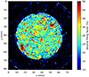 |
Fig. 1. One of the reconstructed images of the CT scan of the spooned sample, showing its inner structure dominated by pebbles of various sizes. The voxel size of the CT scan is 67 μm. The selected slice was taken from the middle of the sample and shows the cylindrical granular water ice surrounded by the cylindrical styrofoam container used as a sample holder during the scans to keep the sample cold. This sample holder has four bulges extending into the sample, as visible in the image. The structure of the styrofoam is visible in the image; however, the colour bar on the right applies only to the water-ice sample. The corners of the image were filled with air during the CT scan and were used as zero-density analogues for the calibration of the scans. The other slices and the poured sample are similar in appearance. |
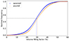 |
Fig. 2. Cumulative distribution of VFFs inside the micro-granular water-ice samples derived from the CT scans. The dotted lines mark the medians of the two distributions for the spooned and poured samples, respectively. |
The granular water-ice sample used in this paper was prepared, as stated above, using a cylindrical sample holder with an inner diameter of 242 mm and a height of 100 mm. On the upper surface of this first sample, and in the middle, we placed an additional micro-granular water-ice sample with a convex hemispherical shape and a diameter of 40 mm. This provides an opportunity to observe the sublimating surface for a longer time before it is progressively obscured due to the formation of a sublimation crater (see Sect. 3). The top part of Fig. 3 shows an image of the sample at a 10° observation angle with respect to the sample surface at the beginning of the experiment. The sample mass was (1.312 ± 0.002) kg, resulting in a VFF of ∼31%. This VFF matches the values derived from the CT scans.
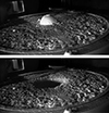 |
Fig. 3. Images of the sample at a 10° observation angle with respect to the sample surface at the beginning (top) and the end (bottom) of the experiment after 47 hours of insolation. In the middle of the sample, we placed a hemispherical granular-water-ice structure with a diameter of 40 mm and the same properties as the entire sample. Over time, a crater formed due to insolation, replacing the convex structure with a concave one. |
3. Experimental results
The sample was exposed to artificial sunlight for approximately 47 hours. As a consequence of the resulting sublimation process, a crater formed and grew deeper over time, gradually reducing the number of instruments able to observe the active surface. Thus, in the following sections, we focus only on the first 11 hours of the experiment, during which the obscuration effect of the crater was insignificant.
We used the data from the scale, permanently measuring the sample mass, and from the infrared camera, observing the spatially resolved surface temperatures of the sample. Additional visible-light cameras were used to observe the dust activity and the evolution of the sample surface.
The main objectives of the measurement are to observe and characterise gas sublimation and the resulting recession of the surface. Fig. 3 (bottom) shows the grown crater at the end of the experiment in the middle of the sample. To our surprise, the sample not only showed the expected persistent gas activity but also a considerable ejection of solid ice particles, which hereafter we refer to as dust activity. The dust activity was present throughout the illumination and reoccurred even after the lamp had been switched off. The activity stopped only at the end of the measurement after 47 hours of insolation, when the crater had grown so deep that the bottom of the sample was reached. A detailed analysis of the gas and dust activity can be found in the following Sects. 3.1 and 3.2.
3.1. Quantifying activity
The total mass evolution over time measured by the scale is shown as a black curve in Fig. 4 and amounts to a mass loss of 13.88 g within a time of 10.37 h during which the illumination was turned on. The mass-reading of the scale fluctuated, and therefore we fitted the mass-loss curve with a cubic polynomial in each time interval between two successive eclipses. The results are indicated by the green curves in Fig. 4, which show that no systematic deviations between the individual measurements and the fit function are present. Additionally, the purple curve shows the integrated mass-loss rate calculated from the spatially resolved temperature data from the infrared camera using the Hertz-Knudsen equation following Gundlach et al. (2011) and the total mass lost amounts to 9.81 g. A moving average was used to smooth the mass-loss rate obtained by the infrared camera before integration. The computation of the mass-loss rate from the infrared camera temperature data with the Hertz-Knudsen equation was previously validated through calibration experiments, whereby we monitored the sublimation rate of a solid water-ice block and granular water ice illuminated with low intensity. In these experiments, no particles were ejected and the calculated mass loss from the infrared camera data and the measured mass loss from the scale were in perfect agreement. The respective mass-loss rates are shown in Fig. 5: those provided by the scale are shown in blue, green crosses show the mean values between eclipses, and those derived from data from the infrared camera are shown in red. The total mass-loss rate is approximately constant, at around 1.32 g/h. The mass-loss rate measured by the infrared camera shows a similar course but with a smaller mass-loss rate of around 0.93 g/h. The grey areas in Figs. 4 and 5 indicate the eclipses.
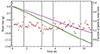 |
Fig. 4. Mass loss of the sample over time measured by the scale (black) and the infrared camera (purple). The brown crosses indicate the fraction of mass loss by particles and the grey areas mark the periods when the lamp was turned off. The green curves between successive eclipses show the cubic-polynomial fit to the noisy scale measurements. |
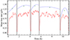 |
Fig. 5. Mass-loss rates measured using the scale (described by the derivatives of the third-order polynomial fit to the measurement data; blue curves with means indicated by green crosses) and the infrared camera (red curve) over time. The grey areas mark the time intervals when the lamp was turned off. |
The mass-loss rate in gas derived from the infrared camera temperature data always lies below the total mass-loss rate measured using the scale (see Fig. 5). This confirms the observation that a certain amount of mass is lost in ejected solid particles. However, both curves show similar behaviour over time (see Fig. 4). The mass-loss rates based on the infrared camera and the scale can be used to calculate the fraction of mass lost as solid particles. The mass-loss fraction of particles is marked with brown crosses in Fig. 4, where the means are 32%, 30%, 23%, 29%, and 29% between the eclipses. The first data point after each eclipse is unreliable because the mass loss does not start directly with the illumination, but after some delay. However, the fit to the scale mass does not account for the data recorded during the eclipse, and thus neglects this delay and overestimates the mass loss at these times. This difference between the mass-loss rate measured by the scale and the infrared camera can be clearly seen in Fig. 5.
3.2. Structural evolution of the sample
The illuminated area is a circle with a diameter of 80 mm. Therefore, not the entire surface area of the sample was subjected to insolation. The whole surface area was observed by multiple cameras before and after the insolation periods, while an image of the illuminated area was taken every 30 seconds. This way, the structural changes in the non-illuminated area can also be analysed. With the images before and after the entire insolation, we verified that the non-illuminated parts of the sample surface do not change and that no significant fallback from ejected particles reaches the sample (see Fig. 3). Thus, all dust activity observed during insolation contributes to the overall mass loss.
The dust activity can be seen in Fig. 6 for three points in time. In the left image, taken towards the beginning of the insolation period, the hemispherical surface is completely visible, while it is nearly gone in the central image, taken five hours into the total insolation. In the right image, recorded towards the end of the 11 hour experiment period described in this paper, a crater has formed.
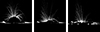 |
Fig. 6. Ejected particles at the beginning of the experiment, and then after five and ten hours of the measurement (from left to right). For each image, 5453 pictures taken at 4000 frames per second were used; all particles were tracked and the tracks were combined into one picture. Because of the low brightness of the escaping particles, we had to overexpose the sample surface; for clarity reasons, we therefore masked out the surface in the images. |
4. Physical interaction between light and sample
In this section, we describe a thermophysical model that is designed to help explain the self-ejection of water-ice particles. We start with a simple energy balance calculation, and then calculate the wavelength-dependent absorption depth of the incoming light. This information is used to model the temperature distribution inside the uppermost layers of the sample. This and the known size distribution of the water-ice particles are input parameters for a model described in Sect. 5 that can explain the self-ejection of granular water ice.
4.1. Global energy balance
During the first five illumination cycles of the experiment, a total of 13.88 g of water ice are lost from the sample, either in solid particles or due to sublimation. However, as we do not see significant fallback, the ejected particles also sublimate outside our viewing area. For the total mass to sublimate, an energy of 38.1 kJ is needed, using a latent heat of sublimation for water ice of 2744 kJ/kg (Hübner et al. 2006). The total input energy from the artificial Sun is ∼520 kJ, meaning that around ∼7% of the input energy is absorbed and turned into sublimation; therefore, ∼93% of the incoming light is scattered or reflected from the sample surface. This finding matches well with albedo measurements for water-ice samples (Henneman & Stefan 1999) over the wavelength range covered by our halogen lamp and shows that the energy balance is coherent. The contribution of the overall heating of the sample is negligibly small compared to the sublimation energy.
4.2. Absorption depth of incoming light
To compute the absorbed power density of the incident light in the ice sample as a function of depth, we employed the dense-medium radiative-transfer approach for a semi-infinite layer of ice particles (Markkanen & Agarwal 2019). This method allows the calculation of scattering and absorption of light in a densely packed particulate random medium, where particle sizes are on the order of the incident wavelength. It relies on the Monte Carlo solution of the radiative-transfer equation, accounting for near-field effects through incoherent input parameters.
The computation was executed as follows: First, we generated N samples of a random medium comprising spherical particles with the given particle size distribution of the granular water ice (Kreuzig et al. 2023) and a packing density of 0.3. We then computed the ensemble-averaged incoherent phase matrix, albedo, mean free path length, and the coherent effective refractive index using the numerically exact fast superposition T-matrix method code (Markkanen & Yuffa 2017), as detailed in Markkanen & Agarwal (2019) (Eqs. (10)–(15)). These computations were performed for wavelengths spanning the spectral range of the light source, that is, 0.40 − 4.00 μm, in 0.01 μm increments. The wavelength-dependent complex refractive index of pure water ice was taken from Warren & Brandt (2008). Third, the incoherent phase matrix, albedo, mean free path, and coherent effective refractive index for each wavelength were used as inputs in the Monte Carlo radiative transfer solver. This resulted in a spectral absorbed power density as a function of depth in a layer of ice particles of 100 mm in thickness. The results can be seen in Fig. 7. Finally, we obtained the total absorbed power density by integrating the spectral density over the wavelength range.
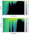 |
Fig. 7. Absorbed power density for different wavelengths in the first 10 mm (top) and 2 mm (bottom) of the sample in W/m2. The colours indicate the logarithm of the absorbed power density, while black indicates that no energy is absorbed. The white curves denote the maximum penetration depth of incoming light as a function of wavelength and have been added to guide the eye. |
4.3. Verification of absorption wavelength range
To constrain the energy absorption in the three main near-infrared (NIR) bands of water ice at 1.5 μm, 2.0 μm, and 3.0 μm (Warren 1984), we performed experiments using the S-Chamber. In those, we placed a layer of liquid water between the artificial Sun and the samples, because liquid water has similar NIR absorption bands to water ice, while being almost transparent at visible (VIS) wavelengths (Ustin & Jacquemoud 2020; Pansini & Varandas 2022). We counted the ejected particles at different times during the illumination using a high-speed camera, which can be seen in Fig. 8. The results show that a 2 mm thick water layer already reduces the solid-particle activity by a factor of roughly 10, and 5 mm of water stop almost all activity. This was further quantified by measuring the masses of the samples before and after a one-hour experiment, which can be seen in Table 1. The mass loss after one hour of insolation is also reduced by a factor of roughly 10 for a water-layer thickness of 1–2 mm, confirming the results from the ejected-particle observations. Both measurements confirm that most of the energy is indeed absorbed in the three NIR absorption bands, which is consistent with the calculations presented in Sect. 4.2.
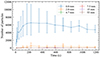 |
Fig. 8. Number of detected particles for different thicknesses of the water layer between the artificial Sun and the sample as a function of time after the start of insolation. The error bars indicate the minimal and maximal measured particle numbers in two to four experimental runs. |
Measured mass loss after one hour of insolation for three different water-layer thicknesses between the artificial Sun and the sample.
4.4. Temperature profile inside the sample
We used an implicit thermophysical model to determine the 1D temperature profile in the middle of the sample at the point of maximum incoming irradiation. The model is based on that described in Gundlach et al. (2020), but we replace the explicit solver of the heat transfer equation with a fully implicit solver and assume only water ice. Furthermore, we added a formulation for the volume absorption of light, following the work of Davidsson & Skorov (2002), allowing the light to penetrate to deeper layers, following the absorption curve discussed in Sect. 4.2. To define the depth to which sublimation occurs, which is where the saturation vapour pressure is achieved, one can account for the pressure drop from the sample’s interior to the surface by considering the mean path length Λ as the characteristic length scale. Following Güttler et al. (2023), their Eq. (6), the mean free path can be calculated via Λ = 2/3 ⋅ dp ⋅ ϵ/(1 − ϵ), with the characteristic particle radius dp and the porosity ϵ = 1 − Φ, with Φ being the VFF. For VFFs of between 0.60 and 0.17, which are the most extreme values achievable with our code, and with dp ≈ 6.6 μm, here using a median mass-equivalent radius of 3.3 μm, this equates to Λ ≈ (2.6 − 21.8) μm. To simplify matters and to speed up the calculations, we only treat sublimation up to depths of the order of Λ, as no net sublimation takes place in the region where the saturation vapour pressure is reached. For this, we assumed that the entire gas emission stems from an uppermost layer of thickness h0, which we determined by equating the total cross section of all ice particles in the volume within the depth h0, taking into account their real size distribution, with the cross section of the considered volume. This allows us to compute the h0 values individually for each realisation of the sphere packing and we therefore favour this approach over using Λ. For the VFFs in the range between 0.17 and 0.60, we get h0 = 23.2 − 6.7 μm; indeed, these values are comparable to the mean free path length Λ. In the layers with depths of h > h0, we assumed that the equilibrium vapour pressure is reached so that no net evaporation takes place. With this in mind, we only considered sublimation in the top five layers of the simulated region, totalling 12.5 μm in depth for the temperature profile simulations with a VFF of 30%. This is roughly the depth needed to match the outgassing of the inner surface to the sample surface.
The resulting temperature profile is shown in Fig. 9. It varies by only 1.1 K in the top 1000 μm. This yields a difference in saturation vapour pressure of 0.02 Pa between the warmest and the coldest layers. As a result, we decided to assume a constant temperature for the modelling of the dust activity (see Sect. 5) given the minimal temperature gradient within the modelled region. We also performed these simulations for a VFF of 40%, which only changed the absolute values, resulting in a peak temperature value of 200.5 K instead of the current peak value of 198.7 K, but changing the VFF has no strong influence on the steepness of the temperature profile. As the model is solely dependent on the geometry, as long as the temperature profile can be assumed to be constant, the actual temperature value chosen for the simulation only changes the simulated timescale.
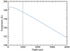 |
Fig. 9. Temperature profile of the thermal simulations of the granular water ice with a VFF of 30% in the blue line. The dashed black line denotes the depth of the z-direction simulation boundary for the geometrical model in Sect. 5. |
5. Deciphering the ‘dust’ activity mechanism using a geometrical model
In our search for the physical process responsible for the dust emission, we can first rule out electrical charging of the surface by the intense illumination. Spectral measurements show that no light with a wavelength of < 400 nm – equivalent to a photon energy of > 3.1 eV – entered the vacuum chamber. As the ionisation energy for water ice is ∼12.6 eV (see e.g. Yabushita et al. 2013), the presence of free surface charges can be excluded.
To understand the dust emission of the pure micro-granular ice sample under insolation, we developed a geometrical model of a small part of the near-surface area of the sample (see Fig. 10 for a schematic description). We modelled the ice particles as spheres with the same mass–frequency distribution as that measured for the same water-ice particles by Kreuzig et al. (2023, see Fig. 8). These spheres were then placed in a cubic volume of 200 × 200 × 1000 μm3 with pre-determined VFFs of between 0.17 and 0.60, following the random ballistic deposition with rolling’ recipe of Klar et al. (2024). Taking into account the results from Sect. 4, we assumed a constant temperature of 200 K for the entire simulated sample (see Fig. 9). For the VFFs in the range between 0.17 and 0.60, we get h0 = 23.2 − 6.7 μm; indeed, these values are comparable to the mean free path length Λ. In the following, we used the formulation of h0 through the particle surface, because this allows us to calculate the value from the actual generated realisation of the particle distribution instead of some mean value. In the layers with depths h > h0, we assume that the equilibrium vapour pressure is reached, and that therefore no net evaporation takes place.
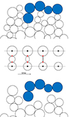 |
Fig. 10. Schematic representation of the geometrical model. Top: 2D representation of the sphere-cluster model, here for simplicity with only three different ice-sphere sizes. Centre: treatment of the evaporation of an ice sphere. A small ice sphere is in contact with two larger neighbours whose centres (marked by the black crosses) are fixed by external processes; for example, by being constrained in a network of other particles. Time proceeds from left to right. In this visualisation, it is assumed that the small sphere in the centre evaporates on a shorter timescale than its two larger neighbours. The red dots mark the contacts between the central sphere and its neighbours, which disappear when the central sphere has evaporated. In the simulations, only the last step (shown on the right) is considered, that is, the evaporation of the ice particles is not explicitly treated. Bottom: after the evaporation of the smallest ice spheres, an isolated cluster (depicted in blue) is detached from the bulk of the sample. This cluster is assumed to be emitted in solid form. |
In the next step, the evaporation lifetime of each water-ice sphere with a location close to the current surface – that is, for h < h0 – was calculated and sorted in ascending order. Each completely evaporated sphere was deleted from the sample (see Fig. 10) and we verified whether or not the loss of contact leads to the isolation of sphere clusters, that is, clusters that are no longer in contact with the rest of the sample. These clusters are then released and their properties (mass and linear dimensions) are recorded, taking into account the reduction in mass by evaporation of all cluster components until the time of release. After each time step, the location of the surface was determined and new ice spheres with h < h0 were allowed to evaporate. This process was repeated until the sample had completely dissolved.
Our model results are shown in Fig. 11, where we plot the calculated dust-emission fraction as a function of the VFF of the simulated sample. The data shown in Fig. 11 display a steep increase in dust activity with decreasing VFF, with dust activity reaching values of up to ∼35% for the lowest VFF of 0.17. For the highest VFF of 0.60, we get only a tiny fraction of dust emission, amounting to ∼2%. We fitted a power law with an exponent of −1.449 and an offset of 0.117 to the data in Fig. 11, obtaining very good agreement with the data. This function was then used to extrapolate the fraction of particle mass loss for VFFs below 0.17 and above 0.60, assuming that the fraction of particle mass loss cannot exceed unity. We reach this value at a VFF of ∼0.15. This threshold value is logical, in that it corresponds to a case in which the mean coordination number of the constituent grains approaches a value of 2 (Klar et al. 2024). When one of these contacts is broken, the agglomerate is detached into two parts, one of which contributes to the dust emission.
Using the real distribution of VFFs as shown in Fig. 2 and the results shown in Fig. 11, we derived the total fraction of particle mass loss for the entire sample by multiplying the mass fraction per VFF bin with the respective ejected fraction of particle mass loss shown in Fig. 11, and summing up all the bins. We obtain a simulated total fraction of particle mass loss of 10.8% for the spooned sample and 8.9% for the poured sample. These values are considerably smaller than the 23–32% measured in our experiments (see Sect. 3.1). However, our simple geometrical model is based on the assumption of zero tensile strength, meaning all neighbouring particles have to be removed before the ejection of the cluster, which is probably an overly pessimistic view. For typical water-ice temperatures at the evaporation front of ∼200 K, the sublimation pressure is on the order of 0.1 Pa. Thus, relaxing the zero tensile strength limit to values in that range will yield higher mass factions in solid-particle ejection. Such simulations, however, are complex and beyond the scope of this paper.
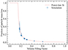 |
Fig. 11. Mass fraction of emitted solid-ice particles as a function of the VFF when applying the geometrical model to the measured particle size distribution of the micro-granular water-ice sample (Kreuzig et al. 2023). Due to the inherent randomness of the sphere placements, five simulations were performed for each VFF. Also shown is a fit to the data that surpasses a dust-emission efficiency of unity at a VFF of ∼0.15 and has been set to 1 for smaller VFF values. The fitting function that was used is y(x) = (x − x0)a ⋅ 10b, with the values a = −1.449, b = −2.185, and x0 = 0.117. |
Our dust-emission model suggests that the ejection of particles is driven by the temperature of the ice and not by any photometric effects caused by the light. In order to prove this, granular water-ice samples were placed in the S-Chamber with the cooling systems inactive so that the samples were much warmer than those in the L-Chamber. The samples were illuminated by the artificial Sun through a water layer of 110 mm in thickness. On the one hand, this ensures that no NIR energy absorption takes place, meaning that particle ejection due to this effect can be ruled out (see Fig. 8), and on the other hand provides the same visible-light illumination conditions necessary to prove the presence or absence of particle emission. Performing these experimental runs, the cameras detected emitted solid particles, proving that temperature is the driving factor behind this effect.
Kossacki et al. (1997) performed experiments with water-ice samples but did not report particle ejection. However, the samples used in that work had a VFF of 65%, which is significantly higher than that of our samples. In order to show that the vast difference in VFF is the cause of this discrepancy, we performed experiments with a compressed and an uncompressed sample with VFFs of 56% and 31%, respectively, in the S-Chamber (see Fig. 12). The top panel of Fig. 12 shows dust activity as a function of time. The compressed sample is active in the beginning but the activity stops after 24 minutes. We attribute the initial activity to the fact that the top layers are less compressed during the sample preparation. Once this layer is removed and the higher VFF in the interior is reached, the activity stops, bringing our finding in agreement with Kossacki et al. (1997).
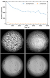 |
Fig. 12. Comparison between compressed and uncompressed granular water-ice samples. Top: Number of detected particles for compressed (VFF 56%) and uncompressed (VFF 31%) granular water ice as a function of time after the start of insolation. Bottom: Surface images of the uncompressed (top images) and compressed (bottom images) granular water-ice samples at the beginning of the insolation phase (left images) and after 96 minutes of illumination (right images). |
6. Relation to real comets
The dust and ice in cometary nuclei may have two morphologies: (i) either dust grains and ice grains form separately in the solar nebula and are then intimately mixed together when the cometary precursor planetesimal forms; or (ii) ice condenses on the surfaces of pre-existing dust grains and thus forms core-mantle particles. In both cases, a dust-emission process sketched by our geometrical model in Sect. 5 is feasible. In the following, we present a more detailed look at these two possibilities.
(i) There is evidence that almost pure water-ice grains exist in comets (Schulz et al. 2006; Protopapa et al. 2014, 2018; Faggi et al. 2021). Thus, an intimate mixture of dust and ice particles seems to be a possibility, and the evaporation of an ice grain next to a dust grain may liberate the dust particle when no other contact exists for that grain or the cluster of grains that it belongs to. As long as the percolation limit for the dust particles is not reached, we expect dust release to be possible if the gas drag dominates over the gravitational pull. For equal-sized dust and ice grains, this percolation limit is reached for a VFF of the dust grains of ∼0.3 (He & Ekere 2004). As this value is close to the overall VFF of cometary nuclei – values in the range of 0.15 − 0.37 were derived for comet 67P (see e.g. Blum et al. 2017) –, we expect that the percolation limit will not be reached for sufficiently low dust-to-ice ratios. This way, the release of dust without the necessity to overcome the cohesion barrier seems possible in principle. In particular, the so-called water-ice-enriched blocks (WEBs; Ciarniello et al. 2022) may fulfil the physical requirements for the emission of small particles. According to Fulle et al. (2020) and Ciarniello et al. (2022), the refractory to water-ice mass ratio in the WEBs is < 5, meaning a refractory to water-ice volume ratio of < 1.7 − 2.5, depending on the mass density of the refractory material. Thus, a substantial share of the volume of the WEBs consists of water ice and the conditions for the validity of our model are present.
(ii) If all particles constituting the cometary nucleus were originally core-mantle grains, and if we assume that a size distribution exists for those grains and that the evaporation timescale is shorter for smaller grains, as in our geometrical model in Sect. 5, each completed ice-shell evaporation leads to the liberation of a refractory core grain. This grain can either be directly dragged by the gas flow into space, if geometrically possible, or will attach to a neighbouring dust particle. This process continues until isolated islands of grain clusters form that are then liberated from the comet nucleus.
Thus, in principle, small dust particles might also be ejected by real cometary nuclei without coming into conflict with the cohesion barrier. In particular, the WEBs are locations with a high chance of being the source of the dust emitted into the tail. However, dedicated numerical simulations are required to reveal the efficiency and limits of this process. This will be the task of a future study.
7. Summary and conclusion
This study focuses on understanding the properties of granular water ice, the most prevalent volatile in comets, in order to improve models of cometary activity. We created a sample of micrometre-sized water-ice particles, placed it in a cryogenic thermal vacuum chamber, and exposed it to high-intensity VIS/NIR illumination. We measured the total mass-loss rate of the sample using a scale and recorded surface temperatures with an infrared camera, while multiple other cameras captured surface changes and solid-particle ejections. Our findings indicate that the energy absorbed in the NIR absorption bands of water ice is sufficient to explain the total mass loss caused by sublimation and solid particle ejection. Between 68% and 77% of the mass loss was due to water-ice sublimation, as derived from surface-temperature measurements. The remaining 23%–32% of the mass-loss rate was due to the ejection of solid ice particles. The self-ejection of water-ice grains can be qualitatively explained by a geometrical model in which solid ice particles are emitted when they lose contact with the sample due to the faster evaporation of connecting smaller ice grains.
These results have potential implications for understanding cometary dust activity. Dust and ice in cometary nuclei may exist in two forms: dust and ice grains form separately and then mix as the cometary precursor planetesimal forms, or ice condenses on dust grains to form core-mantle particles. In both scenarios, a dust-emission process along the lines of our geometrical model is viable. Our findings indicate that small dust particles may be ejected from cometary nuclei without a cohesion barrier, though further numerical simulations are needed to understand the efficiency and limitations of this process.
Acknowledgments
This work was carried out in the framework of the CoPhyLab project funded by the international D-A-CH program (DFG: GU 1620/3-1 and BL 298/26-1, project number 395699456; SNF: 200021E 177964; FWF: I 3730-N36). Further funding was provided by DLR German Space Agency through grant 50WM2254A, by DFG grants BL 298/27-1, project number 436344287 and DFG GU 1620/6-1, project number 493620659 and the European Union under grant agreement NO. 101081937 – Horizon 2022 – Space Science and Exploration Technologies (views and opinions expressed are however those of the authors only and do not necessarily reflect those of the European Union; neither the European Union nor the granting authority can be held responsible for them). J.M. thanks DFG for funding project no. 517146316. In addition, we thank René Laquai, Markus Bartscher and Ulrich Neuschaefer-Rube from the Physikalisch Technische Bundesanstalt (PTB) for providing us with the CT scans of the granular water-ice samples. We thank the anonymous reviewer for their constructive feedback that improved the quality of the paper.
References
- Bischoff, D., Kreuzig, C., Haack, D., Gundlach, B., & Blum, J. 2020, MNRAS, 497, 2517 [CrossRef] [Google Scholar]
- Bischoff, D., Schuckart, C., Attree, N., Gundlach, B., & Blum, J. 2023, MNRAS, 523, 5171 [NASA ADS] [CrossRef] [Google Scholar]
- Blum, J., Gundlach, B., Krause, M., et al. 2017, MNRAS, 469, S755 [Google Scholar]
- Ciarniello, M., Fulle, M., Raponi, A., et al. 2022, Nature Astronomy, 6, 546 [NASA ADS] [CrossRef] [Google Scholar]
- Ciarniello, M., Fulle, M., Tosi, F., et al. 2023, MNRAS, 523, 5841 [CrossRef] [Google Scholar]
- Davidsson, B. J. R., & Skorov, Y. V. 2002, Icarus, 159, 239 [CrossRef] [Google Scholar]
- Faggi, S., Lippi, M., Camarca, M., et al. 2021, AJ, 162, 178 [NASA ADS] [CrossRef] [Google Scholar]
- Fulle, M., Blum, J., & Rotundi, A. 2019, ApJ, 879, L8 [NASA ADS] [CrossRef] [Google Scholar]
- Fulle, M., Blum, J., Rotundi, A., et al. 2020, MNRAS, 493, 4039 [CrossRef] [Google Scholar]
- Gundlach, B., Skorov, Y., & Blum, J. 2011, Icarus, 213, 710 [Google Scholar]
- Gundlach, B., Schmidt, K. P., Kreuzig, C., et al. 2018, MNRAS, 479, 1273 [NASA ADS] [CrossRef] [Google Scholar]
- Gundlach, B., Fulle, M., & Blum, J. 2020, MNRAS, 493, 3690 [NASA ADS] [CrossRef] [Google Scholar]
- Güttler, C., Rose, M., Sierks, H., et al. 2023, MNRAS, 524, 6114 [CrossRef] [Google Scholar]
- Haack, D., Otto, K., Gundlach, B., et al. 2020, A&A, 642, A218 [NASA ADS] [CrossRef] [EDP Sciences] [Google Scholar]
- He, D., & Ekere, N. N. 2004, Journal of Physics D Applied Physics, 37, 1848 [Google Scholar]
- Henneman, H. E., & Stefan, H. G. 1999, Cold Regions Science and Technology, 29, 31 [NASA ADS] [CrossRef] [Google Scholar]
- Hübner, W. F., Benkhoff, J., Capria, M., et al. 2006, Heat and Gas Diffusion in Comet Nuclei (Bern: International Space Science Institute) [Google Scholar]
- Klar, L., Glißmann, T., Lammers, K., Güttler, C., & Blum, J. 2024, Granul. Matter, 26 [CrossRef] [Google Scholar]
- Kossacki, K. J., Kömle, N. I., Leliwa-Kopystyński, J., & Kargl, G. 1997, Icarus, 128, 127 [NASA ADS] [CrossRef] [Google Scholar]
- Kreuzig, C., Kargl, G., Pommerol, A., et al. 2021, Review of Scientific Instruments, 92, 115102 [Google Scholar]
- Kreuzig, C., Bischoff, D., Molinski, N. S., et al. 2023, RAS Techniques and Instruments, 2, 686 [NASA ADS] [CrossRef] [Google Scholar]
- Kreuzig, C., Bischoff, D., Meier, G., et al. 2024, A&A, 688, A177 [NASA ADS] [CrossRef] [EDP Sciences] [Google Scholar]
- Kuehrt, E., & Keller, H. U. 1994, Icarus, 109, 121 [NASA ADS] [CrossRef] [Google Scholar]
- Markkanen, J., & Agarwal, J. 2019, A&A, 631, A164 [NASA ADS] [CrossRef] [EDP Sciences] [Google Scholar]
- Markkanen, J., & Yuffa, A. J. 2017, Journal of Quantitative Spectroscopy and Radiative Transfer, 189, 181 [NASA ADS] [CrossRef] [Google Scholar]
- Pansini, F. N., & Varandas, A. J. 2022, Chemical Physics Letters, 801, 139739 [NASA ADS] [CrossRef] [Google Scholar]
- Protopapa, S., Sunshine, J. M., Feaga, L. M., et al. 2014, Icarus, 238, 191 [NASA ADS] [CrossRef] [Google Scholar]
- Protopapa, S., Kelley, M. S. P., Yang, B., et al. 2018, ApJ, 862, L16 [NASA ADS] [CrossRef] [Google Scholar]
- Schulz, R., Owens, A., Rodriguez-Pascual, P. M., et al. 2006, A&A, 448, L53 [NASA ADS] [CrossRef] [EDP Sciences] [Google Scholar]
- Ustin, S. L., & Jacquemoud, S. 2020, in How the Optical Properties of Leaves Modify the Absorption and Scattering of Energy and Enhance Leaf Functionality, eds. J. Cavender-Bares, J. A. Gamon, & P. A. Townsend (Cham: Springer International Publishing), 349 [Google Scholar]
- Warren, S. G. 1984, Appl. Opt., 23, 1206 [NASA ADS] [CrossRef] [Google Scholar]
- Warren, S. G., & Brandt, R. E. 2008, Journal of Geophysical Research: Atmospheres, 113 [Google Scholar]
- Yabushita, A., Hama, T., & Kawasaki, M. 2013, Journal of Photochemistry and Photobiology C: Photochemistry Reviews, 16, 46 [Google Scholar]
All Tables
Measured mass loss after one hour of insolation for three different water-layer thicknesses between the artificial Sun and the sample.
All Figures
|
Fig. 1. One of the reconstructed images of the CT scan of the spooned sample, showing its inner structure dominated by pebbles of various sizes. The voxel size of the CT scan is 67 μm. The selected slice was taken from the middle of the sample and shows the cylindrical granular water ice surrounded by the cylindrical styrofoam container used as a sample holder during the scans to keep the sample cold. This sample holder has four bulges extending into the sample, as visible in the image. The structure of the styrofoam is visible in the image; however, the colour bar on the right applies only to the water-ice sample. The corners of the image were filled with air during the CT scan and were used as zero-density analogues for the calibration of the scans. The other slices and the poured sample are similar in appearance. |
| In the text | |
|
Fig. 2. Cumulative distribution of VFFs inside the micro-granular water-ice samples derived from the CT scans. The dotted lines mark the medians of the two distributions for the spooned and poured samples, respectively. |
| In the text | |
|
Fig. 3. Images of the sample at a 10° observation angle with respect to the sample surface at the beginning (top) and the end (bottom) of the experiment after 47 hours of insolation. In the middle of the sample, we placed a hemispherical granular-water-ice structure with a diameter of 40 mm and the same properties as the entire sample. Over time, a crater formed due to insolation, replacing the convex structure with a concave one. |
| In the text | |
|
Fig. 4. Mass loss of the sample over time measured by the scale (black) and the infrared camera (purple). The brown crosses indicate the fraction of mass loss by particles and the grey areas mark the periods when the lamp was turned off. The green curves between successive eclipses show the cubic-polynomial fit to the noisy scale measurements. |
| In the text | |
|
Fig. 5. Mass-loss rates measured using the scale (described by the derivatives of the third-order polynomial fit to the measurement data; blue curves with means indicated by green crosses) and the infrared camera (red curve) over time. The grey areas mark the time intervals when the lamp was turned off. |
| In the text | |
|
Fig. 6. Ejected particles at the beginning of the experiment, and then after five and ten hours of the measurement (from left to right). For each image, 5453 pictures taken at 4000 frames per second were used; all particles were tracked and the tracks were combined into one picture. Because of the low brightness of the escaping particles, we had to overexpose the sample surface; for clarity reasons, we therefore masked out the surface in the images. |
| In the text | |
|
Fig. 7. Absorbed power density for different wavelengths in the first 10 mm (top) and 2 mm (bottom) of the sample in W/m2. The colours indicate the logarithm of the absorbed power density, while black indicates that no energy is absorbed. The white curves denote the maximum penetration depth of incoming light as a function of wavelength and have been added to guide the eye. |
| In the text | |
|
Fig. 8. Number of detected particles for different thicknesses of the water layer between the artificial Sun and the sample as a function of time after the start of insolation. The error bars indicate the minimal and maximal measured particle numbers in two to four experimental runs. |
| In the text | |
|
Fig. 9. Temperature profile of the thermal simulations of the granular water ice with a VFF of 30% in the blue line. The dashed black line denotes the depth of the z-direction simulation boundary for the geometrical model in Sect. 5. |
| In the text | |
|
Fig. 10. Schematic representation of the geometrical model. Top: 2D representation of the sphere-cluster model, here for simplicity with only three different ice-sphere sizes. Centre: treatment of the evaporation of an ice sphere. A small ice sphere is in contact with two larger neighbours whose centres (marked by the black crosses) are fixed by external processes; for example, by being constrained in a network of other particles. Time proceeds from left to right. In this visualisation, it is assumed that the small sphere in the centre evaporates on a shorter timescale than its two larger neighbours. The red dots mark the contacts between the central sphere and its neighbours, which disappear when the central sphere has evaporated. In the simulations, only the last step (shown on the right) is considered, that is, the evaporation of the ice particles is not explicitly treated. Bottom: after the evaporation of the smallest ice spheres, an isolated cluster (depicted in blue) is detached from the bulk of the sample. This cluster is assumed to be emitted in solid form. |
| In the text | |
|
Fig. 11. Mass fraction of emitted solid-ice particles as a function of the VFF when applying the geometrical model to the measured particle size distribution of the micro-granular water-ice sample (Kreuzig et al. 2023). Due to the inherent randomness of the sphere placements, five simulations were performed for each VFF. Also shown is a fit to the data that surpasses a dust-emission efficiency of unity at a VFF of ∼0.15 and has been set to 1 for smaller VFF values. The fitting function that was used is y(x) = (x − x0)a ⋅ 10b, with the values a = −1.449, b = −2.185, and x0 = 0.117. |
| In the text | |
|
Fig. 12. Comparison between compressed and uncompressed granular water-ice samples. Top: Number of detected particles for compressed (VFF 56%) and uncompressed (VFF 31%) granular water ice as a function of time after the start of insolation. Bottom: Surface images of the uncompressed (top images) and compressed (bottom images) granular water-ice samples at the beginning of the insolation phase (left images) and after 96 minutes of illumination (right images). |
| In the text | |
Current usage metrics show cumulative count of Article Views (full-text article views including HTML views, PDF and ePub downloads, according to the available data) and Abstracts Views on Vision4Press platform.
Data correspond to usage on the plateform after 2015. The current usage metrics is available 48-96 hours after online publication and is updated daily on week days.
Initial download of the metrics may take a while.