| Issue |
A&A
Volume 693, January 2025
|
|
|---|---|---|
| Article Number | A217 | |
| Number of page(s) | 15 | |
| Section | Stellar structure and evolution | |
| DOI | https://doi.org/10.1051/0004-6361/202452092 | |
| Published online | 21 January 2025 | |
Examining the brightness variability, accretion disk, and evolutionary stage of the binary OGLE-LMC-ECL-14413
1
Universidad de Concepción, Departamento de Astronomía, Casilla 160-C, Concepción, Chile
2
Astronomical Observatory, Volgina 7, 11060 Belgrade 38, Serbia
3
Issac Newton institute of Chile, Yugoslavia Branch, 11060 Belgrade, Serbia
4
Astronomical Observatory, University of Warsaw, Al. Ujazdowskie 4, 00-478 Warszawa, Poland
5
Instituto de Astronomía, Universidad Católica del Norte, Av. Angamos 0610, Antofagasta, Chile
⋆ Corresponding author; This email address is being protected from spambots. You need JavaScript enabled to view it.
Received:
2
September
2024
Accepted:
18
November
2024
Abstract
Context. Several intermediate-mass close binary systems exhibit photometric cycles longer than their orbital periods, potentially due to changes in their accretion disks. Past studies indicate that analyzing historical light curves can provide valuable insights into disk evolution and track variations in mass transfer rates within these systems.
Aims. Our study aims to elucidate both short-term and long-term variations in the light curve of the eclipsing system OGLE-LMC-ECL-14413, with a particular focus on the unusual reversals in eclipse depth. We aim to clarify the role of the accretion disk in these fluctuations, especially in long-cycle changes spanning hundreds of days. Additionally, we seek to determine the evolutionary stage of the system and gain insights into the internal structure of its stellar components.
Methods. We analyzed photometric time series from the Optical Gravitational Lensing Experiment (OGLE) project in I and V bands, and from the MAssive Compact Halo Objects (MACHO) project in the BM and RM bands, covering a period of 30.85 years. Using light curve data from 27 epochs, we constructed models of the accretion disk. An optimized simplex algorithm was employed to solve the inverse problem, deriving the best-fit parameters for the stars, orbit, and disk. We also utilized the Modules for Experiments in Stellar Astrophysics (MESA) software to assess the evolutionary stage of the binary system, investigating the progenitors and potential future developments.
Results. We found an orbital period of 38.15917 ± 0.00054 days and a long-term cycle of approximately 780 days. Temperature, mass, radius, and surface gravity values were determined for both stars. The photometric orbital cycle and the long-term cycle are consistent with a disk containing variable physical properties, including two shock regions. The disk encircles the more massive star and the system brightness variations align with the long-term cycle at orbital phase 0.25. Our mass transfer rate calculations correspond to these brightness changes. MESA simulations indicate weak magnetic fields in the donor star’s subsurface, which are insufficient to influence mass transfer rates significantly.
Key words: stars: activity / binaries: eclipsing / binaries: spectroscopic / circumstellar matter / stars: emission-line / Be / stars: evolution
© The Authors 2025
 Open Access article, published by EDP Sciences, under the terms of the Creative Commons Attribution License (https://creativecommons.org/licenses/by/4.0), which permits unrestricted use, distribution, and reproduction in any medium, provided the original work is properly cited.
This article is published in open access under the Subscribe to Open model. This email address is being protected from spambots. You need JavaScript enabled to view it. to support open access publication.
1. Introduction
Interacting binary stars constitute complex natural laboratories, allowing the study of a wide range of phenomena such as the physics of accretion disks, stellar winds, gas dynamics of mass flows between stars, angular momentum loss and balance, stellar rotation, and the effects of tidal forces. It is believed that a significant portion of stars are members of multiple star systems, and that interactions between closely bound, gravitationally linked stars are common in the Universe. The most energetic phenomena detected so far, such as the merging of black holes or neutron stars, are considered to be the final stages in the evolution of binary systems that have previously undergone phases of mass transfer and angular momentum loss. A good review of binary star evolution is given by Eggleton (2011).
Among the myriad of interacting binary stars, a particularly intriguing group displays a photometric periodicity longer than the orbital period with a typical amplitude at the I band of 0.1 or 0.2 mag, whose nature still defies explanation (Mennickent et al. 2003; Mennickent 2017). These are known as double periodic variable stars (DPVs), with masses of around 10 solar masses and orbital periods ranging from 3 to 100 days. In these systems, there is invariably a B-type dwarf star, enveloped in a gas disk fed by a cooler giant star of approximately one solar mass that fills its Roche lobe. More than 200 DPVs have been reported in the Galaxy and the Magellanic Clouds (Mennickent et al. 2003, 2016; Poleski et al. 2010; Pawlak et al. 2013; Rojas et al. 2021) and the well-studied systems reveal higher luminosities and hotter temperatures than normal Algol-type binaries (Mennickent et al. 2016). Some examples of these systems previously detected in our Galaxy include RX Cas (Gaposchkin 1944), AU Mon (Lorenzi 1980), β Lyr (Guinan 1989), V 360 Lac (Hill et al. 1997) and CX Dra (Koubsky et al. 1998).
It has been proposed that the longer period of DPVs results from variations in the mass transfer rate, modulated by oscillations in the equatorial radius of the donor star, governed by a magnetic dynamo cycle (Schleicher & Mennickent 2017). This would induce observable changes in the gas disk over extended timescales. While a few DPVs have been investigated with high levels of detail and precision, recent analyses of light curves from the Optical Gravitational Lensing Experiment (OGLE) database for specific objects have yielded intriguing insights.
For instance, OGLE-LMC-DPV-097 displays a notable long-term cycle length of ∼306 days, with a significant fluctuation of ∼0.8 magnitudes in the I-band. This system orbits every 7 75 and comprises stars with modest masses of 5.5 and 1.1 M⊙. A key finding from examining OGLE-LMC-DPV-097 is the systematic variation in its orbital light curve throughout the long-term cycle. At the long cycle’s nadir, the secondary eclipse is almost imperceptible, and in the rising phase, the system’s brightness is more pronounced in the first quadrant compared to the second. These observations can be attributed to the variations in the disk’s temperature and dimensions, alongside fluctuations in the luminous and heated spots. The disk’s radius contracts to 7.5 R⊙ at the cycle’s low point and expands to 15.3 R⊙ during the rise, with its outer edge temperature varying from 6870 K to 4030 K between these phases (Garcés et al. 2018).
In examining the photometric characteristics of OGLE-BLG-ECL-157529, we encounter another intriguing scenario. This system is marked by orbital and extended periods of 24.8 days and 850 days, respectively, with stellar masses similar to OGLE-LMC-DPV-097. It is observed that while the primary minimum’s magnitude remains largely stable, the secondary minimum exhibits significant fluctuations. The secondary minimum occurs due to the eclipse of the donor star by the combined structure of the accretor and its disk. This suggests the presence of a fluctuating accretion disk. Notably, the brightness at the orbital phase of 0.25 aligns closely with the long-term cycle. The disk’s fractional radius (Fd), a metric for the accretor’s Roche lobe occupancy, reveals that the disk expands beyond the tidal radius during peak activity and longer cycles. Conversely, Fd decreases below the tidal radius during quicker, less intense long-term cycles in later epochs. In this system, the long-term cycle’s minimum is attributed to a thicker disk that obscures more of the accretor, with a higher mass transfer rate resulting in a hotter disk at the outer edge. The disk’s radius oscillations over hundreds of days defy explanation through viscous energy release, as is seen in the superhumps of precessing disks in cataclysmic variables like SU UMa stars. This is because Lindblad resonance regions lie well outside the disk’s radius. As an alternative, the hypothesis of variable mass injection as a cause of long-term photometric variability has been suggested (Mennickent & Djurašević 2021).
In order to complement the above studies, and provide a much complete picture of the behavior of these DPV systems, we present a photometric study of the eclipsing binary DPV OGLE-LMC-ECL-14413 (Graczyk et al. 2011; Pawlak et al. 2016). This binary is also known as OGLE-III LMC162.7.89414, OGLE-IV LMC503.02.14123, TIC 373520393, MACHO 78.6943.2764, and 2MASS J05232086-6950586 and their data include α2000 = 05 : 23 : 20.96, δ2000 = −69 : 50 : 58.01 and I = 16.817 mag and V = 18.001 mag2. This object was selected because of its relatively long orbital period and peculiar characteristics. The OGLE Collection of Variable Stars Website indicates that the system has an orbital period of 38 1613814. The system is mentioned as a unique DPV among the sample of LMC DPVs studied by Poleski et al. (2010). These authors noticed that apparently the amplitude of the long-term cycle gets smaller during one of the eclipses, and also that the depth of the usually deeper minimum changes from cycle to cycle. They argue that a similar depth of both minima suggests that temperatures of both components are similar and conclude, from the observation that the mean light curve is typical for semi-detached or contact binary systems, that the radius of the donor star is one of the biggest among donors of known DPVs, or that the total mass of the binary is smaller than for the other DPVs. The authors also argue that the donor eclipses the disk and the gainer during the shallower and more stable eclipse.
2. Photometric data and light curve
The photometric time series analyzed in this study consists of 3899 I-band data points and 416 V-band datapoints obtained by the Optical Gravitational Lensing Experiment (OGLE, Udalski et al. 2015). The I-band light curve shows the typical variability of an eclipsing binary, plus a remarkable long-term variability in the upper boundary of the dataset, which is shaped by the brighter datapoints (Fig. 1). In addition, we study 1315 BM and 1510 RM data points obtained by the MAssive Compact Halo Objects (MACHO) project3. The whole dataset, summarized in Table 1, spans a time interval of 30.85 yr.
Photometric observations.
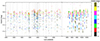 |
Fig. 1. OGLE I-band light curve of OGLE-LMC-ECL-14413. Colors indicate different orbital phases and dashed lines show mid times of the data strings listed in Table 2. |
In this paper, as a starting point, we use the ephemeris for the occultation of the cooler star, provided by the OGLE team (Pawlak et al. 2016, no error is given):
 (1)
(1)
When comparing DPV systems that feature alternating depths of primary and secondary minima, it is crucial to maintain a consistent physical definition of these eclipses. As was mentioned earlier, we have adhered to the methodology established by Pawlak et al. (2016).
In order to check the constancy of the orbital period, we performed an analysis of the times of the primary eclipse using the method of comparison of predicted times with observed times of eclipses, described by Sterken (2005). As eclipse timings we have chosen the fainter points in the colored data strings shown in Fig. 1. We find that the data is compatible with a constant orbital period and there is no practical difference with the ephemerides provided by the OGLE team.
Furthermore, in order to improve the orbital period, we performed an analysis of the main eclipse times. For that, since most eclipses are not well defined individually, and after a visual inspection of the light curve, we selected candidates for minima as those observations with magnitudes at bands I, BM, and RM fainter than 17.4, −5.35, and −6.00 and a few outliers with phases discordant were rejected. The 95 eclipse times thus selected are shown in Table B.1.
Using the published orbital period as a trial, we calculated the cycle numbers for every minimum and fit a straight among the (N, time) pairs obtaining the following improved ephemeris for the main eclipse (Fig. 2):
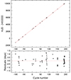 |
Fig. 2. Times of main minima versus cycle number and the best linear fit along with residuals. The slope of the fit gives the orbital period, viz. Po = 38 |


 (2)
(2)
This new orbital period has a difference of 0 00221 with the previously reported period, this accumulates 0
 66 during the 300 cycles of observations, or equivalently 0.017 orbital phase units. We also calculated the orbital period for the OGLE data yielding Po = 38
 159 ± 0
 012 using the Phase Dispersion Minimization software (PDM, Stellingwerf 1978) and Po = 38
 123 ± 0
 095 using the generalized Lomb Scargle software (GLS, Zechmeister & Kürster 2009).
The light curve variability cannot be understood in terms of a two-star system, and the presence of circumstellar matter around the gainer is suggested by the observations (Fig. 3). It is interesting that the eclipse observed at phase 0.0, which sometimes is the deeper one, corresponds to occultation of the donor, since it is the eclipse with larger residuals and inter-epoch variability. The cooler star (the donor) is eclipsed by a variable physical structure. However, the depth of eclipse at phase 0.5 is rather stable, compatible with the stability of the donor and the occultation of the whole disk or a large fraction of it. The roughly constant shape of this eclipse confirms our ephemerides. Furthermore, there is no evidence for changes in the orbital period. The light curve outside the eclipse of the gainer, shows larger scatter before epochs at HJD′ ∼ 8273. On the other hand, at some epochs, the ingress of the eclipse of the donor is delayed, producing an eclipse of asymmetrical shape. These aspects could be attributed to variable amounts of circumstellar mass in the line of sight, considering the interacting nature of this binary discussed later in this paper.
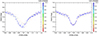 |
Fig. 3. OGLE I-band light curve of OGLE-LMC-ECL-14413 phased with the orbital period around the eclipse of the donor (left) and the gainer (right). Colors indicate different HJDs. |
While the I-band light curve is dense enough to allow a good analysis of orbital and system parameters, the V-band data are scarce, and we used them only for the determination of the color at minimum and the temperature of the donor star. During the secondary eclipse, the color V − I = 1.263 mag. If we take the mean E(V − I) = 0.113 ± 0.060 mag for the LMC (Joshi & Panchal 2019), then we get (V − I)0 = 1.150 ± 0.06 mag, implying T2 = 5100 K, according to the calibration given by Mennickent et al. (2020a). As a reference, the OGLE database provides V − I = 1.156 mag, suggesting T2 = 4982 K, but this value rests on the average color from the entire light curve. We can also use the reddening maps by Skowron et al. (2021) to get E(V − I) = 0.106 ± 0.086 which gives (V − I)0 = 1.157 ± 0.086 mag. We decided to keep the temperature of the donor in T2 = 5000 fixed with an uncertainty of ±200 K, neglecting errors that could come from the disk contribution to the color at the secondary eclipse.
3. Methodology and light curve analysis
In this section, we discuss our model for the light curve based only on OGLE data, since the errors associated with MACHO photometry are ten times larger than those for OGLE data. Therefore, MACHO light curve were used to find additional times of minima only. In order to study the photometric changes, we divided the whole dataset in subsamples of 27 consecutive data sets (Table 2). This allowed us to work with clean orbital light curves with no much influence of the long-term cycle. The choice of a different number of segments does not change the results of this paper. We must keep in mind that the time range must be large enough to include data to represent adequately the orbital light curve, especially eclipses and quadratures, but also short enough to exclude as much as possible the variability due to the long-term cycle.
Data strings.
3.1. The light curve model
Utilizing an advanced simplex algorithm (Dennis & Torczon 1991), the inverse problem was tackled by calibrating the light curve to match the most accurate parameters of the stars-orbit-disk combination for the observed system. The core principles of this model and the procedure for synthesizing light curves are well-documented in the literature (Djurašević 1992, 1996). Further developments and enhancements of this model are also reported (Djurašević et al. 2008) and have been successfully applied in the analysis of numerous close binary systems (e.g., Mennickent & Djurašević 2013; Rosales Guzmán et al. 2018; Mennickent et al. 2020b).
The model quantifies the flux from the binary system as the cumulative output of individual stellar fluxes, coupled with the radiation emanating from an optically thick accretion disk encircling the more luminous star. It incorporates the spatial effects induced by the observer’s viewing angle. The light contribution from the disk is estimated using localized Planck radiation functions at defined temperatures, deliberately omitting the complex calculations involved in radiative transfer. Nevertheless, the model takes into account simpler phenomena like reflection, limb darkening, and gravitational dimming.
The accretion disk is characterized by parameters such as its radius Rd, vertical thickness at its central and outer edges (dc and de, respectively), and a temperature profile that varies with radial distance (e.g., Brož et al. 2021):
 (3)
(3)
where Td signifies the temperature at the disk’s outer rim (r = Rd) and aT is the temperature gradient exponent, constrained to aT ≤ 0.75. The exponent aT indicates the degree to which the radial temperature profile approaches a steady-state configuration (aT = 0.75). This ad hoc radial temperature dependency implies that the disk’s surface is warmer closer to the center and gradually cools with increasing radial distance.
Additionally, the model postulates the presence of two shock regions at the disk’s periphery: a “hot spot” near the conjectured impact point where the gas stream from the inner Lagrangian point collides with the disk, and a “bright spot”, located elsewhere along the disk’s edge. These regions, characterized by variable thickness and temperature compared to the rest of the disk, have been identified in Doppler maps of Algol systems and in hydrodynamic simulations of gas flows in close binary stars (e.g., Albright & Richards 1996; Bisikalo et al. 2000; Atwood-Stone et al. 2012). Their existence was inferred from the analysis of the orbital light curve of the DPV β Lyrae (Mennickent & Djurašević 2013), with interferometric and polarimetric studies further substantiating the presence of the hot spot in this system (Lomax et al. 2012; Mourard et al. 2018). While the genesis of the hot spot is relatively clear, the bright spot’s origin could stem from vertical oscillations of gas at the disk’s outer edge due to interaction with the incoming matter stream (Kaigorodov et al. 2017). The model’s depiction of a singular hot spot on the disk’s edge falls short of accurately representing the intricate and variable nature of the light curves, necessitating the inclusion of the bright spot for a more comprehensive description.
In this model, both the hot and bright spots are defined by their relative temperatures, Ahs ≡ Ths/Td and Abs ≡ Tbs/Td, for their angular dimensions, θhs and θbs, and their angular locations measured from the line joining the stars in the direction of the orbital motion, λhs and λbs. Additionally, θrad represents the angle between the line perpendicular to the local disk edge surface and the direction of maximum radiation from the hot spot. The disk radius is also gauged by the parameter Fd ≡ Rd/Ryk, where Ryk is defined as per Djurašević (1992) as the distance from the center of the hotter star to its Roche lobe, measured perpendicular to the line joining the star centers. In this framework, the disk maintains stability only within the boundary Fd ≤ 1, with any material beyond the Roche limit potentially escaping the system or forming a circumbinary envelope, particularly around the Lagrange equilibrium point L3. The stars’ gravity-darkening coefficients are set at β1 = 0.25 and β2 = 0.08, with albedo coefficients A1 = 1.0 and A2 = 0.5, in accordance with von Zeipel’s law for radiative shells and complete re-radiation (von Zeipel 1924). The limb-darkening for the components was calculated in the way described by Djurašević et al. (2010).
3.2. Results of the light curve model
In studies of over-contact or semi-detached binaries using photometric time series devoid of spectroscopic data, the “q-search” method is commonly employed to deduce the system’s mass ratio, and it is especially precise for eclipsing systems (Terrell & Wilson 2005). Applying this technique, convergent solutions were obtained for a range of mass ratios q = M2/M1, where the subscripts “2” and “1” denote the cooler and hotter stars, respectively. We chose datasets 26 and 27 since they accurately represent the orbital light curve with minimum brightness depressions caused by the disk obscuring the primary star. We performed the search in the mass ratio interval 0.13–0.40 with a step of 0.01 and found that a mass ratio of 0.19 aligns pretty well with these datasets (Fig. 4 and Figs. A.1–A.3). The q error is obtained at the minimum of the S value of the dataset 26. This dataset has a more symmetrical S curve than dataset 27. The 5% S increase from the bottom determines a variation of plus minus 0.01, so we chose a conservative value of ±0.02 for the mass ratio uncertainty. The q value corroborates earlier findings indicating an average q = 0.23 ± 0.05 (std) in previous studies of DPVs (Mennickent et al. 2016). In this paper, we used fg = 84.1 for the gainer and Ω1 and Ω2 equal to 30.702 and 2.208 for the potentials at the gainer and donor surfaces. For that, we assumed synchronous rotation of the donor and non synchronous, critical rotation for the gainer, which fills its critical oval. A second possible model without an accretion disk was not considered, because it leads to an over-contact configuration and requires approximately the same temperatures of the components, which is not in favor of the observations. In addition, the shape of the light curves for this system is typical for systems with an accretion disk, as well as its changes over time. So far, we have analyzed several similar systems (e.g., Rosales et al. 2023; Mennickent et al. 2022). More reason to reject the model without an accretion disk is our experience with the RY Sct system, which we first modeled within such a model, only to later reject this model based on spectroscopic data and re-analyze the observations within the model with an accretion disk (Djurašević et al. 2001, 2008).
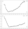 |
Fig. 4. Parameter S = Σ (O-C)2 for the fits done to the light curve of datasets 26 and 27, as a function of mass ratio. |
These datasets were also instrumental in determining the main stellar and orbital parameters. For that, we estimated the mass of the donor star, viz. 1.1 M⊙, by assuming a temperature of T2 = 5000 K and applying the corresponding relationships from the Lang tables (Lang 1993) that indicate a spectral type G5 for a luminosity class III star. Utilizing the derived mass ratio, we then calculated the mass of the primary star, which amouts to 5.8 M⊙. Additionally, we employed Kepler’s third law to determine the orbital separation between the two stars, 90.73 R⊙. All derived stellar and orbital parameters, along with their errors, are shown in Table 3. Estimates for the errors of mass, radius, surface gravity and orbital separation are given in the Appendix.
Calculated stellar and orbital parameters.
We kept constant these stellar and orbital parameters for other datasets, focusing the analysis on the variability of disk parameters. The outcomes of the light curve modeling are detailed in Table B.2. Uncertainties were estimated with numerical experiments around the best fitting values. They must be observed as generic ones due to the non homogenous character of the data. Single orbital light curve fittings are presented in Figs. A.1–A.3, highlighting measurement uncertainties, typical orbital variations, long-term variability, fitting quality, and the system’s visual representation. Observed discrepancies exceeding individual data point errors could be attributed to underestimation of formal errors or unaccounted variabilities in the model. For instance, a possible additional light source is not considered. Another possible cause for these discrepancies could be the span of individual light curves over multiple orbital cycles, introducing long-term variability into the analysis. To address this, a “sliding” polynomial of lower degree was fitted through each light curve segment, with magnitudes at orbital phases 0.25 and 0.75 measured using the corresponding orbital phases and fit values (Table 2).
We find that the disk radius ranges from 31.97 R⊙ to 43.81 R⊙, whereas the disk temperature ranges from 3258 K to 4217 K. The disk outer vertical thickness span from 6.1 to 12.9 R⊙ while the disk height at the inner boundary span from 3.1 to 5.0 R⊙. The hot spot temperature is on average 1.28 ± 0.08 times higher than the surrounding disk and the bright spot is 1.14 ± 0.04 times higher than the surrounding disk. The hot and bright spots are located at 327 2 ± 12
 1 and 94
 5 ± 33
 3, respectively, as measured from the line joining the stars, from the donor to the gainer, and in the sense of the binary motion. The hot and bright spots span arcs of 18
 6 ± 3
6 ± 3 1 and 43
 0 ± 5
0 ± 5 5, respectively, in the disk’s outer edge. In general, we do not observe correlations between the fit parameters except for a few cases.
3.3. A simple model for the mass transfer rate
We also calculated an approximation for the mass transfer rate Ṁ, using the following prescription (Mennickent & Djurašević 2021):
![Mathematical equation: $$ \begin{aligned} \frac{\dot{M}_{2,f}}{\dot{M}_{2,i}}= \frac{ {{R}^2_{\mathrm{disk},f}} [A_{\mathrm{hs},f}T_{\mathrm{disk},f}]^{4} d_{e,f} \theta _{\mathrm{hs},f} }{{{R}^2_{\mathrm{disk},i}} [A_{\mathrm{hs},i}T_{\mathrm{disk},i}]^{4} d_{e,i} \theta _{\mathrm{hs},i}}. \end{aligned} $$](/articles/aa/full_html/2025/01/aa52092-24/aa52092-24-eq24.gif) (4)
(4)
This equation allows us to estimate relative mass transfer rates at different epochs, i and f, for a given system. In order to normalize our determined values of Ṁ, we used as reference its minimum value, attained at the orbital cycle represented by string 19. These values are shown in Table 2, and an uncertainty of up to 40% is derived from the classical formula of error propagation. The mass transfer rate hence calculated has a mean value of 2.06 with a standard deviation of 0.73, and maximum and minimum values of 3.71 and 1.
3.4. The long-term cycle
In order to investigate the long-term cycle length, we searched for periodicities in the data of magnitudes at phase 0.25 with the aid of the GLS periodogram. We searched between 200 and 1500 days, and find a prominent peak at 784 8 ± 24
 3 (Fig. 5). The magnitudes at phase 0.25 follows a long-term tendency. A sinus fit provides overall I-band amplitude of 0.036 ± 0.006 mag although the peak to peak distance is 0.107 mag (Fig. 6).
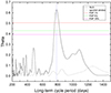 |
Fig. 5. Generalized Lomb Scargle periodogram for the magnitudes measured at phase 0.25. The vertical line shows the maximum value at 784 |

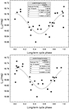 |
Fig. 6. Magnitudes at phase 0.25 phased with the period of 784 |


The long-term cycle is also revealed in the weighted wavelet Z transform (WWZ) as defined by Foster (1996). The WWZ works in a similar way to the Lomb-Scargle periodogram providing information about the periods of the signal and the time associated with those periods. It is very suitable for the analysis of non-stationary signals and has advantages for the analysis of time-frequency local characteristics. We notice that the WWZ transform for the I-band time series suggests a stable long-term cycle length of 780 days, confirming our finding in the periodogram constructed with magnitudes taken around orbital phase 0.25 (Fig. 7). The period obtained every step of 100 days with the above tool shows a distribution with a mean of 778 8 ± 4
8 ± 4 6 (std). A sinus fit provides overall I-band amplitude of 0.037 ± 0.006 mag and basically the same chi square that the case for the period 784
 8 (Fig. 6).
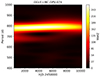 |
Fig. 7. WWZ transform showing a strong signal around 778.8 days. |
In the following, and based on the trial ephemerides shown in Fig. 6, we use as ephemeris for the maximum of the long-term cycle:
 (5)
(5)
Regarding long-term trends, we observe that the disk temperature increases with heliocentric julian date, while the disk radius decreases. Additionally, we find that the disk tends to be hotter when it is smaller (Fig. 8). Throughout the observation period, the mass transfer rate roughly increases (Fig. 9). This observation should be interpreted considering data collected at similar phases of the long-term cycle. It is especially evident in the data colored with blue in the above figure (Φl = 0.87–0.99). Beyond this overarching trend, the parameter dM/dt also mirrors the long-term cycle, as we shall demonstrate next.
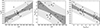 |
Fig. 8. Behavior of some disk parameters according to our models. Typical errors are 60 K and 0.1 R⊙. Best linear fits are shown along with gray light and dark gray regions indicating 95% prediction and confidence bands, respectively. Parameters for these fits are given in Table 4. |
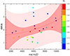 |
Fig. 9. Mass transfer rate versus the mid HJD′ given in Table 2 with colors indicating ranges of the long-term cycle phase. The best quadratic fit, y = (1.59055)+(5.948E-6)*x + (1.06792E-8)*x2 is shown, along with light and dark shaded regions indicating 95% prediction and confidence bands, respectively. |
We notice that the magnitude at orbital phase of 0.25 mirrors the dynamics of the long-term cycle, similarly to how the mass transfer rate does, as shown in Figure 10. Both parameters undergo clear changes throughout the long-term cycle, although with significant scatter. Notably, the peak of the long-term cycle nearly aligns with the maximum in the mass transfer rate, and both curves exhibit a slight shift where the mass transfer rate (Ṁ) precedes the system’s brightness. This suggests a causal relationship: an increase in mass transfer rate leads to an increase in system brightness. The enhanced brightness during the peak of the long-term cycle could result from reduced obscuration of the gainer star and a hotter disk, as is implied by the dc and Rdisk diagrams in Fig. 11. In the same figure, we observe that the hot spot position moves closer to the line joining the stars around Φl = 0.3.
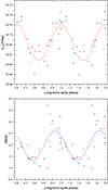 |
Fig. 10. Ṁ and I-band magnitude, measured at orbital phase 0.25, as a function of the long-term cycle phase, based on the analysis of the light curve strings of Table 2. Red (black) dots correspond to data of datasets whose time span is longer (shorter) than 35% of the cycle length. Best sinus fits are also shown. |
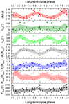 |
Fig. 11. Behavior of some disk parameters during the long-term cycle. Polynomial fits of degree 9th are shown to illustrate tendencies. |
Interestingly, the long-term tendency of disk radius can be observed in the polar diagram of Fig. 12. We see that larger disk are found at the earliest epochs, whereas smaller disk can be found at later epochs. It is at earlier epochs when the bright spot attains larger extension and it is distributed over a wider area in the outer disk.
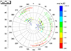 |
Fig. 12. Radial position and angular extension of hot spot (open circles) and bright spot (dots) at different epochs. |
4. On the evolutionary stage
We used the Modules for Experiments in Stellar Astrophysics (MESA), a powerful and widely used suite of open-source computational tools designed for astrophysical research (Paxton et al. 2011, 2015). In particular, when studying binary star evolution, MESA is extremely useful due to its robust and detailed simulations of stellar physics. Crucial for binary star evolution, MESA can simulate interactions between the stars, such as mass transfer, common envelope phases, and tidal effects. These interactions significantly influence the evolution and fate of binary systems. For our purposes, we customize MESA following Rosales et al. (2024), matching the scenario of mass transfer by Roche lobe overflow between two intermediate mass stars.
We performed several trials with initial stellar masses in a range 3.4–5.8 M⊙ for the donor and 1.0–3.4 M⊙ for the gainer, both with step of 0.05 M⊙ and orbital periods in a range 1–10 days with step 1.0 day, allowing the systems to evolve from its initial condition. We fixed the metallicity to Z = 0.006, roughly representative for the Large Magellanic Cloud (Eggenberger et al. 2021). We constructed models that were compared with the observed system properties. Among these models, we selected those that minimized the χ2 parameter, representing mean deviations of the system parameters regarding those of theoretically calculated values. Following Rosales et al. (2024), the prescription for mass transfer considered the fraction of mass lost from the vicinity of donor as fast wind as 1E-3, the fraction of mass lost from the vicinity of accretor as fast wind as 1E-4 and no mass lost from a possible circumbinary matter. The first two parameters were allowed to vary from 1E-1 to 1E-12 in steps of 1 dex. These values were chosen as representative of a case with very small or neglectable mass loss, considering that the more evolved donor should have a wind larger than the B-type dwarf. In other words, we considered quasi-conservative models. The mixing length parameters for donor and gainer were allowed to vary from 0.3 to 1.9 in steps of 0.1 and the final values chosen were 1.0 both. The parameter for semi convection was fixed to 0.01. The above values guarantee an effective convective mixing of chemical species. In order to explore magnetism in the donor star, we activate rotation in the MESA code, enabling also thermohaline mixing. On the contrary, in order to keep simple and fast the calculations, we assumed zero rotation for the gainer switching off this mode.
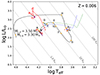 |
Fig. 13. Evolutionary paths of the donor and the gainer for the best model. Model initial and best-fit mass values are shown, along with letters indicating the evolutionary stages described in Table 5. |
Evolutionary stages of OGLE-LMC-ECL-14413.
Our studies showed that the present day binary parameters can be reproduced by a binary of initial period 7 days and initial masses 3.5 and 3.3 M⊙ and current age 200.54 Myr. The evolution of the best model is summarized in Table 5, at specific evolutionary stages labeled accordingly, and from the zero-age main sequence (ZAMS) to 4He depletion.
The stellar and system parameters found compare well with those reported in Table 3; namely, theoretical masses 5.6 and 1.2 M⊙ versus 5.8 and 1.1 M⊙ calculated radii of 23.0 and 3.8 R⊙ versus 22.4 and 3.6 R⊙ and orbital period 38 16 versus 38
 16. Regarding the luminosities, the theoretical temperatures are log T = 3.72 and 4.29 K, versus log T = 3.70 and 4.27 K. We notice a small discrepancy with the luminosity of the gainer, and this principally produces the mismatch between the observed data and the predicted position (X2 stage) in Fig. 13. This is observed even at trials with metallicities of Z = 0.02 and 0.003. It can, in principle, be attributed to the presence of the disk, which hides the more massive star and whose influence in the flux balance has not been included in the MESA calculations. For the same reason, we observe our simulations as general insight of the possible evolutionary path for the binary, and we do not pursue a better approximation, although it is remarkable that the best model is in fact found in a mass transfer stage, with dM/dt = 3.5 × 10⁻⁶ M⊙/yr. The donor is found after hydrogen depletion and with important helium enhancement in its core, while the gainer has rejuvenated acquiring 2.3 M⊙ during the accretion process (Table 5 and Fig. 14). The system already passed by the optically thick mass transfer stage and now it is in a milder stage of mass transfer. During the binary evolution, the donor increased its radius from 2.2 R⊙ to 23 R⊙ and the orbital period increased from 7
 0 to the current value of 38
 16. The Hertzsprung-Russell (HR) diagrams show the huge decrease in the temperature of the donor star, and the increase in the luminosity of the gainer, until reaching the current stage. They also show an expected decrease in the hydrogen and the increase in the helium fraction in the core of the gainer and the donor (Fig. 14). Furthermore, our MESA simulations shows, as expected, how the temperature of the donor evolves first at a nuclear timescale and then, after filling the Roche lobe, at a much shorter thermal timescale when mass transfer occurs. The same for the donor radius, which slightly increases during millions of years to change abruptly, after starting the mass transfer process (Fig. 15).
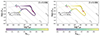 |
Fig. 14. HR diagrams indicating the system evolution along with the hydrogen and helium fractions in the stellar cores. |
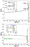 |
Fig. 15. Evolution of the radius and temperature of the donor. (Up): Evolution of the donor star size with an initial mass of 3.5 M⊙ in the binary system OGLE-LMC-ECL-14413, with a companion that has an initial mass of 3.3 M⊙, showing the phases in which cases A, B, and C of RLOF can occur, depending on the age of the system. The inversion of the 1H/4He ratio (X1 stage) is represented by a yellow dot, the mass transfer (E stage) by a blue dot, and the current stage of the system (X2 stage) by a red dot. (Down) Effective temperature Teff as function of age for OGLE-LMC-ECL-14413. We show that the donor star, after crossing the Hertzsprung gap during the onset the blue loop (Stages C and D), follows an evolutionary track until reaching its current stage (X2 stage) on a thermal timescale. This continues until reaching the final stage of non-optically thick mass transfer (H-stage), stopping shortly before Helium depletion. |
We find the system in a mass transfer stage, returning from a huge burst of mass transferred to the gainer at maximum rate of 1 × 10⁻⁴ M⊙/yr; at present time the rate of mass transfer has slowed to dM/dt = 3.46 × 10⁻⁶ M⊙/yr. The overall process, from stages E to H, will last about 655 000 years (Fig. 16).
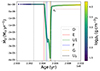 |
Fig. 16. Mass transfer rate versus the system’s age for the best model. Vertical lines indicate the evolutionary stages described in Table 5. The density in the core of the donor star is also shown. |
We further analyze the internal structure of both the donor and the gainer stars using Kippenhahn diagrams (Fig. 17). For the case of the donor, which starts from the ZAMS until helium depletion X(Hec) < 0.2, we were able to identify that the convective zone of the donor star is below 0.5 M⊙ while mostly all nuclear production occurs below 1 M⊙. Additionally, both zones of convection and nuclear production gradually decrease as the system evolves and approaches mass transfer as expected (E stage). Zones of thermohaline instability activation intermittently appear at different stages of evolution. In addition, the overshooting zone is present only until mass transfer occurs and then disappears once mass transfer begin.
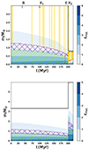 |
Fig. 17. Kippenhahn diagrams showing the internal structure of the donor (up) and gainer (down) stars. Diagrams with initial masses 3.5 and 3.3 M⊙ are shown. The evolutionary calculations were stopped when the donor star reached core helium depletion X(Hec) < 0.2. The x axis gives the age after ignition of hydrogen in units of Myr. The different layers are characterized by their values of M/M⊙. The convection mixing region is represented by hatched green, semi convection mixing region in red and the overshooting mixing region in crosshatched purple. The red dots represent the He core mass, while the thermohaline mixing region is represented in hatched yellow. The solid black lines show the surfaces of the stars. |
For the gainer star, we identified a convective zone from its center to 0.5 M⊙ with a nuclear production rate zone that remains largely unchanged for most of its lifetime from the ZAMS to moments prior to mass transfer (E-stage). In addition, we identified an overshooting zone from 0.7 to 0.9 M⊙. However, after mass transfer, its convective core immediately grew twice the original size, in terms of total mass. Following this, the overshooting zone appears between 1.5 and 2.0 M⊙. Additionally, the nuclear production zone increased significantly, occurring within a central mass of 3 M⊙ after mass transfer.
We calculated the magnetic field structure due to the Taylor-Spruit (ST) dynamo, in particular the toroidal and poloidal components, which resulted in the order of a few Gauss in the stellar subsurface. On the other hand, the Eulerian diffusion for mixing and the Spruit-Taylor diffusion coefficient and the angular velocity were also calculated and are shown in Fig. 18. The magnetic fields obtained with the ST prescription, on the order of a few Gauss, are too weak to be detected observationally with the current usual instrumentation.
 |
Fig. 18. Profiles of magnetic fields generated by the Tayler-Spruit dynamo in the poloidal Br and toroidal Bt components for the donor star at different evolutionary stages. The profiles represent the stages of inversion of the 1H/4He ratio (X1 stage, left panel), the start of mass transfer (E-stage, middle panel) and the current stage (X2, right panel). The Eulerian diffusion coefficient for mixing is represented in orange color, the Spruit-Tayler (ST) diffusion coefficient by the brown line, the poloidal magnetic field as a black line, the toroidal magnetic field in green, whereas the angular momentum is represented in blue and the angular velocity in red. |
5. Discussion
Before we proceed with the interpretation of our results, it’s important to be aware of the limitations of our model. A key simplification is our focus exclusively on circumstellar material within the disk, thereby overlooking any light contributions originating from regions above or below the disk plane. Additionally, we have assumed the gainer is surrounded by an accretion disk, disregarding other potential light sources such as jets, winds, and outflows. Nonetheless, the model allows for the possibility of accounting for variations in disk emissivity that are dependent on azimuthal position through the inclusion of two disk spots. Despite these constraints, and drawing on prior research on algols with disks, our model likely captures the principal light sources for the continuum light. This is evidenced by the close correspondence between the model light curve and the orbital and long-term light curves over the span of 21.7 years of observation (the time covered by the I-band OGLE time series). In addition, we run evolutionary models and find the best one reproducing the present state of the system. Although the match is not perfect, we can certainly infer that the system is product of the evolution of a stellar pair that experienced strong mass transfer in the past, or is still in a semidetached stage with Roche lobe overflowing.
The fractional radius of the gainer is R1/a = 0.04. This value reveals that there is enough room around the gainer for the formation of an accretion disk, since for the system mass ratio, the accreting star is smaller than the circularization radius, where a particle released at the inner Lagrangian point arrives to conserve its angular momentum (Lubow & Shu 1975). The low value of the fractional radius is due to the large orbital separation and long orbital period of this system and it is consistent with the existence of an accretion disk inferred from the light curve model. It is comparable to the value obtained for the long period system V495 Cen (Rosales Guzmán et al. 2018; Rosales et al. 2021). Interestingly, in OGLE-LMC-ECL-14413, the disk vertical height near the star is larger than twice the gainer radius, provoking a significant occultation of the star.
During the 30.85 year time baseline the system shows systematic changes of disk properties, in particular its vertical height at the outer edge. In hydrostatic equilibrium, the vertical height, H, of an accretion disk at radius Rd is:
 (6)
(6)
where vk is the Keplerian velocity and cs the sound speed, which for an isothermal perfect gas can be approximated as:
 (7)
(7)
(Eqs. (3.35) and (3.32) in Kolb 2010). Using the mean parameters at the outer and inner disk we get (vk, cs) = (164, 6.1) and (552, 13.7) in km s−1, respectively, yielding H/R = 0.04 and 0.02. Considering the averages de/Rd = 0.23 and dc/R1 = 1.15 and that the vertical thickness is twice H, we conclude that the disk vertical height is larger than expected for hydrodynamical equilibrium, at the inner and outer boundaries, suggesting that turbulent motions dominate the disk vertical structure. In this context, it may be worth mentioning that in a detailed model of β Lyrae, the disk height had to be multiplied by a factor about 4 times its expected equilibrium value, possibly reflecting non-negligible hydrodynamic flows within the disk (Brož et al. 2021). These turbulent motions could be produced by the continuos injection of mass from the inner Lagrangian point, through a gas stream, into the accretion disk. Incidentally, the variable thick disk explains why the primary and secondary eclipses relative depth reverses, since part of the gainer is hidden by the disk that masks its luminosity to a variable degree. In addition, the variable projected disk area into the visual line of sight contributes to occult a fraction of the donor while it is eclipsed. The low contribution of the gainer to the total flux is reproduced by our models as shown in Figs. A.1–A.3.
In principle, the disk can be stable until the last non-intersecting orbit defined by the tidal radius (Paczynski 1977; Warner 1995, Eq. (2.61)):
 (8)
(8)
we get Rt/aorb = 0.50, or Rt = 45.4 R⊙. We observe that during all the observing epochs the disk outer radius keeps inside the volume defined by the tidal radius.
The value of the mass transfer rate found 3.5 × 10⁻⁶ M⊙/yr, must be consensual with the constancy of the orbital period. For a binary system ongoing conservative mass transfer, we should expect a change of the orbital period of (Huang 1963):
 (9)
(9)
This means a change of 2.9 × 10⁻⁴ days per year, or 8.9 × 10⁻³ days during the whole observing window. This is not observed, therefore the actual mass transfer rate is smaller than 3.5 × 10⁻⁶ M⊙/yr or systemic mass loss is important for the angular momentum balance.
As was stated previously, a magnetic dynamo in the donor has been invoked as the origin of the long-term cycle. The idea behind this scenario is that the dynamo produces cyclic changes in the equatorial radius of the donor star, enhancing quasi-periodically the amount of mass transferred onto the gainer. This should produce effects in the accretion disk, which is exposed to cycles of enhanced mass transfer. These effects could be changes in the disk radius, height or even disk temperature. An insight favoring the dynamo hypothesis is the discovery that the donor dynamo number increases during epochs of high mass transfer in DPVs (Mennickent et al. 2018; San Martín-Pérez et al. 2019). In addition, the calculated long period for OGLE-LMC-ECL-14413, according to the formula given by Schleicher & Mennickent (2017), is 820 days, close to the values obtained from the periodograms and the WWZ analysis. However, our MESA analysis shows that the magnetic fields, at least those calculated from the Spruit-Taylor prescription, are usually less than a thousand Gauss; that is, too low to produce observable effects, as we shall now show.
It has been shown that fluctuations in the radius of a star can be attributed to the gravitational interaction between the orbit and changes in the configuration of a magnetically active star within the binary system. As the star progresses through its activity cycle, variations in the distribution of angular momentum lead to the star’s changing shape. Variations in the overfill factor of the Roche lobe should produce changes in mass transfer rate. This was proposed as a possible origin for the DPV long-term cycles by Schleicher & Mennickent (2017). The change in the stellar radius ΔR = Rnew − R, derived from the prescription of Applegate (1992, Eqs. (7) and (23)) is given by:
 (10)
(10)
where B is the subsurface magnetic field strength. On the other hand, the expected mass transfer rate is given by (Ritter 1988):
 (11)
(11)
where Ṁ0 is the mass transfer rate when B = 0, and it can be assumed as constant, whereas H2 is the pressure scale height in the Roche potential given by:
 (12)
(12)
where k is the Boltzmann constant, T the donor temperature, mp the proton mass, g the local acceleration of gravity, and μ is the mean molecular weight, assumed 1.23 for a star in the LMC with Z ≈ 0.01. In addition, from equations 8 and 9 we get:
 (13)
(13)
Considering values of R = 22.42 R⊙, M = 1.1 M⊙, and T = 5000 K, we get H2 = 56 284 560 m; that is, R/H2 = 277.4. If we furthermore consider a subsurface magnetic field strength of 10 kG, we get a fractional radius change, ΔR/R, on the order of 7.3E-6 and a change in mass transfer rate by a factor exp(2.06E-3); that is, negligible. Therefore, we need larger magnetic field strengths than those produced by the Spruit-Taylor mechanism in the donor subsurface to produce appreciable changes in mass transfer rates and in particular, to reproduce the broad range of values shown in Table 2. New investigations of the 3D internal magnetic structure and its dependence on rapid rotation and its temporal evolution should be important to shed light on the importance of stellar magnetism for the DPV long-term cycles, possibly following the techniques and methodologies developed by Navarrete et al. (2023).
6. Conclusion
We have investigated the intriguing light curve of the DPV OGLE-LMC-ECL-14413, spanning 30.85 years. Our model successfully reproduces the overall I-band light curve, capturing both the orbital variability with a periodicity of 38 16 and the DPV cycle, which has a duration of approximately 780 days and exhibits a full amplitude of 0
 076 at the I-band. This model includes the light contribution from an accretion disk, characterized by an average radius of 38 R⊙, and two hot shock regions located at the outer disk edge. Additionally, for the first time, we have measured fundamental stellar parameters for this system. Our findings include stellar components with masses of 5.8 ± 0.3 and 1.1 ± 0.1 M⊙, radii of 3.6 ± 0.1 and 22.4 ± 0.8 R⊙, and temperatures of 18701 ± 208 K and 5000 ± 200 K, respectively. These stars are separated by a distance of 90.7 ± 1.8 R⊙, and exhibit surface gravities (log g) of 4.08 ± 0.04 and 1.78 ± 0.03.
Our findings trace the evolutionary history of the system, revealing that it is currently experiencing a burst of mass transfer as the donor fills its Roche lobe. We also observe significant changes in the disk’s vertical height, suggesting that turbulent motions contribute to the disk’s vertical extension. The system comprises a B-type dwarf, approximately spectral type B3, accreting matter from a cooler, K5-type giant star, according to the spectral classification scheme given by Harmanec (1988). Our MESA simulations, employing the Spruit-Taylor prescription for magnetism, indicate only weak magnetic fields on the cooler star’s subsurface, insufficient to account for the observed changes in mass transfer rate.
In terms of the broader context of DPVs, our work aligns with previous studies such as those of OGLE-LMC-DPV-097 and OGLE-BLG-ECL-157529 (Garcés et al. 2018; Mennickent & Djurašević 2021), which have also noted long-term changes in accretion disk properties that influence the orbital light curve’s shape. Specifically, the maximum brightness during the long-term cycle in both OGLE-BLG-ECL-157529 and OGLE-LMC-ECL-14413 can be attributed to less obscuration of the gainer by a thinner, hotter disk, thereby increasing the visible surface of the gainer. For OGLE-LMC-ECL-14413, the most significant finding is that the long-term cycle could be driven by changes in mass transfer rate, as illustrated in Fig. 10, and that the peak of the long-term cycle occurs when the disk is hotter and thinner.
The DPV phenomenon is both fascinating and inherently complex. Future investigations involving high spectral resolution data and decade-long time series are poised to illuminate this phenomenon further. Moreover, new theoretical simulations that leverage increased computational power will enhance our understanding of these binary systems.
Data availability
Figs. A1–A3 are available at: https://doi.org/10.5281/zenodo.14192345
Acknowledgments
We thanks an anonymous referee for the useful comments and suggestions on the first version of this manuscript. We acknowledge support by the ANID BASAL project Centro de Astrofísica y Tecnologías Afines ACE210002 (CATA). This research has made use of the SIMBAD database, operated at CDS, Strasbourg, France. This work has been co-funded by the National Science Centre, Poland, grant No. 2022/45/B/ST9/00243.
References
- Albright, G. E., & Richards, M. T. 1996, ApJ, 459, L99 [NASA ADS] [Google Scholar]
- Applegate, J. H. 1992, ApJ, 385, 621 [Google Scholar]
- Atwood-Stone, C., Miller, B. P., Richards, M. T., Budaj, J., & Peters, G. J. 2012, ApJ, 760, 134 [NASA ADS] [CrossRef] [Google Scholar]
- Bisikalo, D. V., Harmanec, P., Boyarchuk, A. A., Kuznetsov, O. A., & Hadrava, P. 2000, A&A, 353, 1009 [NASA ADS] [Google Scholar]
- Brož, M., Mourard, D., Budaj, J., et al. 2021, A&A, 645, A51 [EDP Sciences] [Google Scholar]
- Dennis, J. E., & Torczon, V. 1991, SIAM J. Optimization, 1, 448 [CrossRef] [Google Scholar]
- Djurašević, G. 1992, Ap&SS, 196, 267 [Google Scholar]
- Djurašević, G. 1996, Ap&SS, 240, 317 [Google Scholar]
- Djurašević, G., Zakirov, M., Eshankulova, M., & Erkapić, S. 2001, A&A, 374, 638 [NASA ADS] [CrossRef] [EDP Sciences] [Google Scholar]
- Djurašević, G., Vince, I., & Atanacković, O. 2008, AJ, 136, 767 [Google Scholar]
- Djurašević, G., Latković, O., Vince, I., & Cséki, A. 2010, MNRAS, 409, 329 [CrossRef] [Google Scholar]
- Eggenberger, P., Ekström, S., Georgy, C., et al. 2021, A&A, 652, A137 [NASA ADS] [CrossRef] [EDP Sciences] [Google Scholar]
- Eggleton, P. 2011, Evolutionary Processes in Binary and Multiple Stars (Cambridge, UK: Cambridge University Press) [Google Scholar]
- Foster, G. 1996, AJ, 112, 1709 [NASA ADS] [CrossRef] [Google Scholar]
- Gaposchkin, S. 1944, ApJ, 100, 230 [NASA ADS] [CrossRef] [Google Scholar]
- Garcés, L. J., Mennickent, R. E., Djurašević, G., Poleski, R., & Soszyński, I. 2018, MNRAS, 477, 11 [Google Scholar]
- Graczyk, D., Soszyński, I., Poleski, R., et al. 2011, Acta Astron., 61, 103 [Google Scholar]
- Guinan, E. F. 1989, Space Sci. Rev., 50, 35 [NASA ADS] [CrossRef] [Google Scholar]
- Harmanec, P. 1988, Bull. Astron. Inst. Czechoslovakia, 39, 329 [Google Scholar]
- Hill, G., Harmanec, P., Pavlovski, K., et al. 1997, A&A, 324, 965 [NASA ADS] [Google Scholar]
- Huang, S.-S. 1963, ApJ, 138, 471 [NASA ADS] [CrossRef] [Google Scholar]
- Joshi, Y. C., & Panchal, A. 2019, A&A, 628, A51 [NASA ADS] [CrossRef] [EDP Sciences] [Google Scholar]
- Kaigorodov, P. V., Bisikalo, D. V., & Kurbatov, E. P. 2017, Astron. Rep., 61, 639 [NASA ADS] [CrossRef] [Google Scholar]
- Kolb, U. 2010, Extreme Environment Astrophysics (Cambridge University Press) [Google Scholar]
- Koubsky, P., Harmanec, P., Bozic, H., et al. 1998, Hvar Obs. Bull., 22, 17 [NASA ADS] [Google Scholar]
- Lang, K. 1993, Astronomy, 21, 95 [Google Scholar]
- Lomax, J. R., Hoffman, J. L., Elias, N. M., Bastien, F. A., & Holenstein, B. D. 2012, ApJ, 750, 59 [CrossRef] [Google Scholar]
- Lorenzi, L. 1980, A&A, 85, 342 [NASA ADS] [Google Scholar]
- Lubow, S. H., & Shu, F. H. 1975, ApJ, 198, 383 [NASA ADS] [CrossRef] [Google Scholar]
- Mennickent, R. E. 2017, Serb. Astron. J., 194, 1 [NASA ADS] [CrossRef] [Google Scholar]
- Mennickent, R. E., & Djurašević, G. 2013, MNRAS, 432, 799 [NASA ADS] [CrossRef] [Google Scholar]
- Mennickent, R. E., & Djurašević, G. 2021, A&A, 653, A89 [NASA ADS] [CrossRef] [EDP Sciences] [Google Scholar]
- Mennickent, R. E., Pietrzyński, G., Diaz, M., & Gieren, W. 2003, A&A, 399, 47 [Google Scholar]
- Mennickent, R. E., Otero, S., & Kołaczkowski, Z. 2016, MNRAS, 455, 1728 [NASA ADS] [CrossRef] [Google Scholar]
- Mennickent, R. E., Schleicher, D. R. G., & San Martin-Perez, R. 2018, PASP, 130 [Google Scholar]
- Mennickent, R. E., Garcés, J., Djurašević, G., et al. 2020a, A&A, 641, A91 [NASA ADS] [CrossRef] [EDP Sciences] [Google Scholar]
- Mennickent, R. E., Djurašević, G., Vince, I., et al. 2020b, A&A, 642, A211 [NASA ADS] [CrossRef] [EDP Sciences] [Google Scholar]
- Mennickent, R. E., Djurašević, G., Petrović, J., et al. 2022, A&A, 666, A51 [NASA ADS] [CrossRef] [EDP Sciences] [Google Scholar]
- Mourard, D., Brož, M., Nemravová, J. A., et al. 2018, A&A, 618, A112 [NASA ADS] [CrossRef] [EDP Sciences] [Google Scholar]
- Navarrete, F. H., Käpylä, P. J., Schleicher, D. R. G., & Banerjee, R. 2023, A&A, 678, A9 [NASA ADS] [CrossRef] [EDP Sciences] [Google Scholar]
- Paczynski, B. 1977, ApJ, 216, 822 [CrossRef] [Google Scholar]
- Pawlak, M., Graczyk, D., Soszyński, I., et al. 2013, Acta Astron., 63, 323 [NASA ADS] [Google Scholar]
- Pawlak, M., Soszyński, I., Udalski, A., et al. 2016, Acta Astron., 66, 421 [Google Scholar]
- Paxton, B., Bildsten, L., Dotter, A., et al. 2011, ApJS, 192, 3 [Google Scholar]
- Paxton, B., Marchant, P., Schwab, J., et al. 2015, ApJS, 220, 15 [Google Scholar]
- Poleski, R., Soszyński, I., Udalski, A., et al. 2010, Acta Astron., 60, 179 [NASA ADS] [Google Scholar]
- Ritter, H. 1988, A&A, 202, 93 [NASA ADS] [Google Scholar]
- Rojas, García G., Mennickent, R., Iwanek, P., et al. 2021, ApJ, 922, 30 [Google Scholar]
- Rosales, J. A., Mennickent, R. E., Djurašević, G., et al. 2021, AJ, 162, 66 [NASA ADS] [CrossRef] [Google Scholar]
- Rosales, J. A., Mennickent, R. E., Djurašević, G., et al. 2023, A&A, 670, A94 [NASA ADS] [CrossRef] [EDP Sciences] [Google Scholar]
- Rosales, J. A., Petrović, J., Mennickent, R. E., et al. 2024, A&A, 689, A154 [NASA ADS] [CrossRef] [EDP Sciences] [Google Scholar]
- Rosales Guzmán, J. A., Mennickent, R. E., Djurašević, G., Araya, I., & Curé, M., 2018, MNRAS, 476, 3039 [Google Scholar]
- San Martín-Pérez, R. I., Schleicher, D. R. G., Mennickent, R. E., & Rosales, J. A. 2019, Boletín de la Asociación Argentina de Astronomía, 61, 107 [Google Scholar]
- Schleicher, D. R. G., & Mennickent, R. E. 2017, A&A, 602, A109 [NASA ADS] [CrossRef] [EDP Sciences] [Google Scholar]
- Skowron, D. M., Skowron, J., Udalski, A., et al. 2021, ApJS, 252, 23 [Google Scholar]
- Stellingwerf, R. F. 1978, ApJ, 224, 953 [Google Scholar]
- Sterken, C. 2005, ASP Conf. Ser., 335, 3 [Google Scholar]
- Terrell, D., & Wilson, R. E. 2005, Ap&SS, 296, 221 [NASA ADS] [CrossRef] [Google Scholar]
- Udalski, A., Szymański, M. K., & Szymański, G. 2015, Acta Astron., 65, 1 [NASA ADS] [Google Scholar]
- von Zeipel, H. 1924, MNRAS, 84, 702 [Google Scholar]
- Warner, B. 1995, Cambridge Astrophys. Ser., 28 [Google Scholar]
- Zechmeister, M., & Kürster, M. 2009, A&A, 496, 577 [CrossRef] [EDP Sciences] [Google Scholar]
Appendix A: Error estimates
We estimate the errors of mass, radius and orbital separation assuming an uncertainty in the temperature and using an analytical approach. The luminosity follows the Stefan-Boltzmann law:
 (A.1)
(A.1)
where R is the radius of the star, σ is the Stefan-Boltzmann constant, and T is the effective temperature. Now, an error in the temperature, ΔT, affects the luminosity due to the dependence L ∝ T4. If we make an error ΔT in measuring the effective temperature of the star, the relative error in the luminosity will be:
 (A.2)
(A.2)
Given that for a main sequence star L ∝ Mα, an error in the luminosity, ΔL, translates into an error in the mass, ΔM, as follows:
 (A.3)
(A.3)
If we use α≈ 3.5 for a main sequence star, and consider that for a giant star the exponent should be larger because of the increasing radius, the relative error in the mass of the donor would be:
 (A.4)
(A.4)
On the other hand, the orbital separation in a binary system is given by Kepler’s third law:
 (A.5)
(A.5)
An error in the stellar masses affects the orbital separation as follows:
 (A.6)
(A.6)
Assuming the relative error is similar for both stars, we can write:
 (A.7)
(A.7)
For α > 3.5:
 (A.8)
(A.8)
From the above equations, and assuming a temperature uncertainty of 4%, we get masses with uncertainty of less than 5% and orbital separation with uncertainty of less than 2%.
To calculate the error in the radius of the giant star filling its Roche lobe, we need to consider how the errors in the mass ratio (q = M1/M2) and the orbital separation (a) affect the error in the Roche lobe radius (RL).
Recall that the Roche lobe radius is given by the empirical Eggleton formula:
 (A.9)
(A.9)
To find the error in RL (the Roche lobe radius, which will approximately be the radius of the giant star), we applied the formula for error propagation. This allows us to calculate the error in RL as a function of the errors in q and a.
Since RL depends on two variables, q and a, the error in RL, denoted as ΔRL, can be computed using the following error propagation formula:
 (A.10)
First we calculate the partial derivative with respect to q:
 (A.11)
Then, we calculate the partial derivative with respect to a. The dependence of RL on a is straightforward, as RL ∝ a. Thus:
 (A.12)
For q = 0.19 with an associated error of 0.02, and assuming a 4% relative error in the orbital separation, we obtain a relative error of 3.54% for the Roche Lobe radius, which also corresponds to the donor star’s radius.
If the gainer follows a mass-radius relationship M ∝ Rβ with β between 0.57 and 0.7, we get the fractional error in the gainer radius less than 0.7 times the fractional error in the gainer mass. If this last is 5%, then the gainer fractional radius uncertainty is less than 4%.
Finally, the surface gravity in solar units is given by:
 (A.13)
where log g⊙ is the solar surface gravity. The error is given by:
 (A.14)
Using the fractional errors quoted above, we derive the errors for log g given in Table 3.
Appendix B: Additional material
Epochs of main eclipses (HJD - 2450000).
Parameters of the light curve fits.
All Tables
All Figures
|
Fig. 1. OGLE I-band light curve of OGLE-LMC-ECL-14413. Colors indicate different orbital phases and dashed lines show mid times of the data strings listed in Table 2. |
| In the text | |
|
Fig. 2. Times of main minima versus cycle number and the best linear fit along with residuals. The slope of the fit gives the orbital period, viz. Po = 38 |
| In the text | |
|
Fig. 3. OGLE I-band light curve of OGLE-LMC-ECL-14413 phased with the orbital period around the eclipse of the donor (left) and the gainer (right). Colors indicate different HJDs. |
| In the text | |
|
Fig. 4. Parameter S = Σ (O-C)2 for the fits done to the light curve of datasets 26 and 27, as a function of mass ratio. |
| In the text | |
|
Fig. 5. Generalized Lomb Scargle periodogram for the magnitudes measured at phase 0.25. The vertical line shows the maximum value at 784 |
| In the text | |
|
Fig. 6. Magnitudes at phase 0.25 phased with the period of 784 |
| In the text | |
|
Fig. 7. WWZ transform showing a strong signal around 778.8 days. |
| In the text | |
|
Fig. 8. Behavior of some disk parameters according to our models. Typical errors are 60 K and 0.1 R⊙. Best linear fits are shown along with gray light and dark gray regions indicating 95% prediction and confidence bands, respectively. Parameters for these fits are given in Table 4. |
| In the text | |
|
Fig. 9. Mass transfer rate versus the mid HJD′ given in Table 2 with colors indicating ranges of the long-term cycle phase. The best quadratic fit, y = (1.59055)+(5.948E-6)*x + (1.06792E-8)*x2 is shown, along with light and dark shaded regions indicating 95% prediction and confidence bands, respectively. |
| In the text | |
|
Fig. 10. Ṁ and I-band magnitude, measured at orbital phase 0.25, as a function of the long-term cycle phase, based on the analysis of the light curve strings of Table 2. Red (black) dots correspond to data of datasets whose time span is longer (shorter) than 35% of the cycle length. Best sinus fits are also shown. |
| In the text | |
|
Fig. 11. Behavior of some disk parameters during the long-term cycle. Polynomial fits of degree 9th are shown to illustrate tendencies. |
| In the text | |
|
Fig. 12. Radial position and angular extension of hot spot (open circles) and bright spot (dots) at different epochs. |
| In the text | |
|
Fig. 13. Evolutionary paths of the donor and the gainer for the best model. Model initial and best-fit mass values are shown, along with letters indicating the evolutionary stages described in Table 5. |
| In the text | |
|
Fig. 14. HR diagrams indicating the system evolution along with the hydrogen and helium fractions in the stellar cores. |
| In the text | |
|
Fig. 15. Evolution of the radius and temperature of the donor. (Up): Evolution of the donor star size with an initial mass of 3.5 M⊙ in the binary system OGLE-LMC-ECL-14413, with a companion that has an initial mass of 3.3 M⊙, showing the phases in which cases A, B, and C of RLOF can occur, depending on the age of the system. The inversion of the 1H/4He ratio (X1 stage) is represented by a yellow dot, the mass transfer (E stage) by a blue dot, and the current stage of the system (X2 stage) by a red dot. (Down) Effective temperature Teff as function of age for OGLE-LMC-ECL-14413. We show that the donor star, after crossing the Hertzsprung gap during the onset the blue loop (Stages C and D), follows an evolutionary track until reaching its current stage (X2 stage) on a thermal timescale. This continues until reaching the final stage of non-optically thick mass transfer (H-stage), stopping shortly before Helium depletion. |
| In the text | |
|
Fig. 16. Mass transfer rate versus the system’s age for the best model. Vertical lines indicate the evolutionary stages described in Table 5. The density in the core of the donor star is also shown. |
| In the text | |
|
Fig. 17. Kippenhahn diagrams showing the internal structure of the donor (up) and gainer (down) stars. Diagrams with initial masses 3.5 and 3.3 M⊙ are shown. The evolutionary calculations were stopped when the donor star reached core helium depletion X(Hec) < 0.2. The x axis gives the age after ignition of hydrogen in units of Myr. The different layers are characterized by their values of M/M⊙. The convection mixing region is represented by hatched green, semi convection mixing region in red and the overshooting mixing region in crosshatched purple. The red dots represent the He core mass, while the thermohaline mixing region is represented in hatched yellow. The solid black lines show the surfaces of the stars. |
| In the text | |
|
Fig. 18. Profiles of magnetic fields generated by the Tayler-Spruit dynamo in the poloidal Br and toroidal Bt components for the donor star at different evolutionary stages. The profiles represent the stages of inversion of the 1H/4He ratio (X1 stage, left panel), the start of mass transfer (E-stage, middle panel) and the current stage (X2, right panel). The Eulerian diffusion coefficient for mixing is represented in orange color, the Spruit-Tayler (ST) diffusion coefficient by the brown line, the poloidal magnetic field as a black line, the toroidal magnetic field in green, whereas the angular momentum is represented in blue and the angular velocity in red. |
| In the text | |
Current usage metrics show cumulative count of Article Views (full-text article views including HTML views, PDF and ePub downloads, according to the available data) and Abstracts Views on Vision4Press platform.
Data correspond to usage on the plateform after 2015. The current usage metrics is available 48-96 hours after online publication and is updated daily on week days.
Initial download of the metrics may take a while.