| Issue |
A&A
Volume 666, October 2022
|
|
|---|---|---|
| Article Number | A51 | |
| Number of page(s) | 15 | |
| Section | Stellar structure and evolution | |
| DOI | https://doi.org/10.1051/0004-6361/202244074 | |
| Published online | 05 October 2022 | |
Cyclic changes in the interacting binary RX Cassiopeiae
1
Universidad de Concepción, Departamento de Astronomía, Casilla 160-C, Concepción, Chile
e-mail: This email address is being protected from spambots. You need JavaScript enabled to view it.
2
Astronomical Observatory Belgrade, Volgina 7, 11060 Belgrade, Serbia
3
Issac Newton institute of Chile, Yugoslavia Branch, 11060 Belgrade, Serbia
4
Institut für Astrophysik, Georg-August-Universität, Friedrich-Hund-Platz 1, 37077 Göttingen, Germany
5
Konkoly Thege Astronomical Institute, Research Center for Astronomy and Earth Sciences, Konkoly Thege Miklós út 15-17, 1121 Budapest, Hungary
6
Inst. de Astronomia, Geofisica e Ciencias Atmosféricas, Universidade de Sao Paulo, Rua do Matao, 1226, Sao Paulo 05508-090, Brazil
Received:
20
May
2022
Accepted:
22
July
2022
Abstract
We analyzed 109 years of published photometry and times of minima of the eclipsing interacting binary RX Cas. The inclusion of 171 previously unnoticed minima confirms the tendency of an increase in the orbital period at a rate of 1.84 s per cycle. We also find evidence of variations in the length of the previously reported long photometric cycle and changes in the shape of the orbital light curve. By modeling the orbital light curves at different epochs, and assuming symmetry in the system physical conditions during the first and second halves of the long cycle, we find that the changes in the orbital light curve can be explained by variations in the physical properties of the accretion disk. We find that epochs of maximum brightness are those of thicker and hotter disks. In addition, we explore the evolutionary history of the system using the Modules for Experiments in Stellar Astrophysics code and find that the binary can be the result of nonconservative evolution of two stars of very similar initial mass (around 5.5 M⊙) and orbital period of 4 days, although less massive and conservative models of longer starting orbital periods cannot be discarded.
Key words: binaries: eclipsing / binaries: spectroscopic / binaries : close / stars: evolution
© R. E. Mennickent et al. 2022
 Open Access article, published by EDP Sciences, under the terms of the Creative Commons Attribution License (https://creativecommons.org/licenses/by/4.0), which permits unrestricted use, distribution, and reproduction in any medium, provided the original work is properly cited.
This article is published in open access under the Subscribe-to-Open model. This email address is being protected from spambots. You need JavaScript enabled to view it. to support open access publication.
1. Introduction
Interesting physical phenomena occur when the more massive star in a binary pair, after expanding due to nuclear evolution, fills its Roche-lobe. Mass flows through the inner Lagrange point from the “donor” star onto the “gainer” star in the form of a gas stream, sometimes forming, after some revolutions, an accretion disk around it. This configuration alters significantly the evolution of the binary compared with the expected evolutionary path for single stars, changing the stellar masses on relatively short timescales and modifying the distribution of angular momentum in the system. Although this process is generally well understood, some important uncertainties remain. The amount of mass loss from the system is not well constrained (Deschamps et al. 2015). It is also not clear if the acceleration of the mass gaining star reaches the critical velocity impeding more accretion or if tidal forces slow down the gainer allowing it to increase its mass (Pols et al. 1991; Gies 2007). Disk masses in these systems are rarely documented and the possible existence of self-gravitating disks around objects like β Lyrae has been speculated (Wilson 2018). This author provides a theoretical framework for a disk of mass around 4% its central star, whereas dynamical instability and unrealistically low viscosity have been mentioned against the existence of a massive disk around β Lyrae (Hubeny et al. 1994).
The basic physics for binary interaction and evolution was described in terms of the Roche model for binary systems (Roche 1873; Kopal 1959) and later on the dynamics of the gas overflowing the Roche lobe and the eventual formation of an accretion disk was explored (Lubow & Shu 1975). The evolutionary sequence of a semidetached system was first explained by Crawford (1955) and later confirmed via evolutionary calculations by Kippenhahn & Weigert (1967) and Eggleton & Kisseleva-Eggleton (2006). The Roche lobe overflow can happen during the donor main sequence stage (case A), during the transition to (or in) the red-giant phase (case B), or during the supergiant phase (case C) (Kippenhahn & Weigert 1967). A more recent review of close binary evolution is provided by Eggleton (2006).
One of the interesting eclipsing binary systems in the northern hemisphere is RX Cassiopeiae (RX Cas, BD+67 244, 2MASS J03074573+6734387, α2000 = 03:07:45.75, δ2000 = +67:34:38.61, V = 8 64, Spectral Type K III+A5 e III)1. It has a distance based on the Gaia DR3 parallax of 1.82 ± 0.03 mas (i.e., 549 [+10 −8] pc) (Pourbaix 2019). The variability of RX Cas was discovered in 1904 by L. Ceraski (Ceraski 1904). Two years later S. Blažko found that the variability is of the Algol type, and provided the ephemeris for the main eclipse considering an orbital period of 32.315 days (Blažko 1906).
The light curve constructed from photographic and visual observations shows a variation with a long period of 517 6 and a range of 0.46 mag (Gaposchkin 1944). A changing orbital period ΔP/Po = 0.86 × 10⁻⁶ has been reported (Kreiner 1978). Earlier attempts to model the light curve assuming a semicontact configuration, and excluding the influence of circumstellar matter, yielded discrepant results for the stellar masses and the mass ratio (Strupat 1987). It is now accepted that the system is characterized by a mid-B 5.8 ± 0.5 M⊙ star of radius ∼2.5 R⊙ and a cooler component of spectral type K1 III of 1.8 ± 0.4 M⊙ and radius 23.5 ± 1.2 R⊙. The hotter star is obscured by a cool geometrically and optically thick accretion disk probably fed by mass transfer from the cooler star (Andersen et al. 1989). The evolutionary stage of this binary was explored suggesting an origin in a binary separated by 345 R⊙ with stellar masses of 7 and 5 M⊙ (Pustylnik et al. 2007). The analysis of photometric time series obtained at different long-cycle epochs indicates a hotter disk (and eventually also a hotter gainer) during the bright stage (Djurašević 1993). The above findings suggest a very active interacting binary where intensive and possibly variable mass transfer is happening. The presence of high-excitation emission lines in the ultraviolet spectrum suggests the presence of a hot corona-like structure, probably fed by a high mass transfer rate, suggesting a system found shortly after mass ratio reversal (Plavec 1980; Andersen et al. 1989). For these reasons, the system might be an ideal target for testing theories of close binary star evolution during stages of mass transfer and interaction. Interestingly, and possibly related to this condition, the excesses at λ 3.5 and 5 microns are attributable to the emission of an optically thin circumstellar dust shell with a grain temperature ∼600–700 K. With a luminosity of ∼3 × 1033 erg s−1, the radius of the dust shell is reported to be ∼4.6 × 1014 cm (Taranova & Shenavrin 1997).
At the same time that large-scale multiband photometric surveys and high-precision satellite photometry offer exciting and new opportunities for the study of close binaries undergoing interaction processes, the study of earlier archival data for relevant targets can provide important insights into the mass transfer or loss processes on timescales of decades or even centuries. In this study we hope to contribute to the understanding of the RX Cas system by providing (1) an updated view of the photometry available for this target, considering contemporaneous ground-based and satellite photometric data along with ancient archival photometric data; (2) a new study of the orbital photometric variability and the reported long-cycle variability; (3) new constraints on orbital period variability and stellar and orbital parameters; and (4) a general discussion of the evolutive stage and possible causes for the enigmatic long cycle.
The paper is organized as follows. In Sect. 2 we give details of the photometric observations analyzed in this paper. In Sect. 3 we present our results based on photometric studies. In Sect. 4 we present the light curve model and the stellar and disk physical parameters. In Sect. 5 we discuss the evolutionary stage of the binary. In Sect. 6 we discuss the system under the framework of close binary star evolution, and in Sect. 7 we summarize our conclusions.
2. Observations
2.1. Photometric time series based on archive data
The photometric data used in this paper were collected from several previously published articles and publicly available databases. We studied the photometric time series found in the All-Sky Automated Survey for Supernovae (ASAS-SN)2 in V and g (Shappee et al. 2014; Kochanek et al. 2017), and the data from the Kamogata Kiso Kyoto Wide-field Survey (KWS; Maehara 2014) in Ic and V. In addition, we included data acquired with the Optical Monitoring Camera (OMC, Mas-Hesse et al. 2003) on board the high-energy INTEGRAL satellite, which provides photometry in the Johnson V band for sources brighter than around V ∼ 18 mag. (Domingo et al. 2010). Archival observations of the American Association of Variable Star Observers (AAVSO) were also examined (Kafka 2021) along with HIPPARCOS data (Perryman et al. 1997). Based on all these datasets and other data published or provided by several researchers, we present for the first time an analysis of 5794 V-band measurements of RX Cas spanning 42 542 days (116.5 years). Measurements earlier than HJD 2446479 provided Julian days for the magnitudes; we have transformed them into heliocentric Julian days. Some of the old data that were reported as “brightness” or “photographic magnitudes” were shifted to the mean of the modern KWS V-band dataset. A few magnitudes reported as differential values were shifted to the V-scale using the reported V-band magnitude of the comparison star. The HIPPARCOSHp magnitudes were transformed to V-band magnitudes using the equations provided by Harmanec (1998). For that we used B − V = 1.5 from SIMBAD3 and we neglected the third-order coefficient multiplying U − B in their formula. This is a rough approximation, since it neglects the B − V variability, but allows a first-order approximation to the V light curve; an error of 0 03 in B − V would result in a 0
 01 error in V (Harmanec 1998). No exact transformation is possible due to the lack of simultaneous UBV colorimetry. On the other hand, we used V = 9
 73 for the comparison star BD+67 243, following SIMBAD, to make a small correction to the measurements provided by Haas (1924). All these pre-adjustments of the data do not modify timings of minima, but must be taken into consideration when evaluating large strings of data, especially those merging different data sources. Modern data, especially those obtained from satellites, do not suffer from this limitation. A summary of the V-band photometric data considered in this paper, along with references to the data sources are given in Table 1, and Ic- and g-band data are reported in Table 2.
Photometric V-band time series analyzed in this paper.
Photometric Ic- and g-band time series analyzed in this paper.
A view of the overall V-band light curve long-term variability, labeling different datasets, is shown in Fig. 1. A zoomed-in image of two distinct time ranges illustrating epochs of eclipses and general variability is shown in Fig. 2. The comparison between V-, I-, and g-band light curves is shown in Fig. 3.
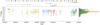 |
Fig. 1. V magnitudes from the datasets listed in Table 1 during the whole range of observing dates. Data distributions and their fits are shown on the right side. The typical error for a single data point is 0.01 mag. |
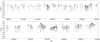 |
Fig. 2. Close-up of V magnitudes from the datasets listed in Table 1 during selected ranges of observing dates. The typical error for a single data point is 0.01 magnitude. |
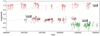 |
Fig. 3. Magnitudes from the KWS-I and ASAS-SN V and g datasets. The typical error for a single data point is 0.01 magnitude. |
2.2. WISE and 2MASS infrared photometry
We searched for infrared magnitudes in the NASA/IPAC infrared science archive4. We investigated the Wide-field Infrared Survey Explorer (WISE), a NASA medium-class explorer mission that conducted an all-sky survey at mid-infrared bandpasses centered around wavelengths 3.4, 4.6, 12, and 22 μm (hereafter W1, W2, W3, and W4; Wright et al. 2010). The survey was conducted with a 40 cm cryogenically cooled telescope in a sun-synchronous polar orbit. Four infrared detectors imaged the same sky field of view over 7.7 s (W1, W2) and 8.8 s (W3, W4). Here we use the data from the second-pass processing, obtained with improved calibration and processing algorithms, superseding those obtained for the preliminary data release. According to the survey documentation, WISE profile-fitting photometry reliably extracts measurements of saturated sources using the nonsaturated wings of their profiles up to brightnesses of approximately 2.0, 1.5, −3.0, and −4.0 mag in W1, W2, W3, and W4.
We also investigated the Two Micron All Sky Survey (2MASS) database (Skrutskie et al. 2006). This astronomical survey ran from 1997 to 2001 on the entire sky at near-infrared wavelengths using two automated 1.3-m telescopes, one located in the northern hemisphere and the other in the southern hemisphere. The survey provided J-, H-, and K-band magnitudes whose respective photometric broadband filters have transmission curves centered at 1.25, 1.65, and 2.17 microns.
2.3. Search for minima
We investigated the Lichtenknecker5 database of the German Association of Variable Stars (BAV), which lists 126 minima of RX Cas between 2416250.9000 and 2455040.8000, from different sources, based on CCD photometry, photoelectric data, photographic plates, and visual photometry. We find that 42 of these minima were secondary eclipse minima and therefore were not considered in our analysis of the main eclipse timings. We added five main eclipse times between 2444208.68 and 2446827.389 reported by Andersen et al. (1989). In addition, we searched for minima in the sources mentioned in Tables 1 and 2, considering V- and g-band data. We could not find the minima using parabolic fits or similar methods due to sparse data, and for the same reason we do not have error estimates for the new minima times. We thus considered a data point as a minimum at the V band and before HJD 2435000 when V < 9.6 mag, and between this date and HJD 2450000 when V < 9.4 mag; after that date we considered V < 9.45 mag. The small differences in threshold magnitudes account for the long-term tendencies observed in the light curves. In this way and after rejecting 58 data points as secondary eclipse minima or outliers, we added 157 new main eclipse times in the V band to the list of previously known timings. For ASAS-SN g-band data we used the limit g < 10.2 mag obtaining 14 main eclipse minima. The 171 new minima are given in Table 3.
New photometric timings identified with minima for the main eclipse.
3. Results
3.1. Rate of the orbital period change
We performed an analysis of observed (O) minus calculated (C) primary eclipse times (Sterken 2005). We have
 (1)
(1)
where Po is the orbital period and N the cycle number. After some trials we decided to use for the linear ephemerides the test zero point HJD0 = 2416248.781 and the orbital period Po = 32 3238 (Fig. 4). We find that the O–C can be fit with the parabola:
 (2)
(2)
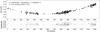 |
Fig. 4. Observed minus calculated times of minima, normalized to the test period Po = 32 |

Since we include in our calculation minima times with and without published errors, we use unweighted times for the O–C fit. An a posteriori estimate for the typical error of the new minima is 0.48 days, derived from the residuals in Fig. 4. Hence the main eclipse minima is
 (3)
(3)
We know that twice the second-order coefficient gives us the rate of period change, in this case 1.84 s per cycle, basically confirming the value of 1.81 s per cycle previously reported (Andersen et al. 1989). This means that in 115 years (about 1300 cycles), the orbital period increases by 0 028 days (i.e., 40 min or 0.09%). A list with quadratic ephemerides reported in the literature is given in Table 4.
Reported quadratic ephemerides for the main minimum of RX Cas.
3.2. Search for additional photometric periods
We searched for additional periods in the seven consecutive data strings indicated in Table 5. These were chosen because of their high data clumping and lack of significant data gaps. We used the phase dispersion minimization algorithm (PDM; Stellingwerf 1978), adequate for light curves of eclipsing binaries showing prominent main and secondary eclipses, to find average orbital periods and their errors for every data string. In addition, using the generalized Lomb–Scargle (GLS; Zechmeister & Kürster 2009) periodogram, we detected the previously reported long periodicity in all data strings except the first. The long periodicity appears as a brightness oscillation on a timescale of 700 days in the second data string, as a cyclic modulation of length 356 days in the third data string, and as a periodic signal of about 516 days in the subsequent data strings (Fig. 5). All these long periods were detected with a high level of significance. We find that the long cycle is present on timescales of decades with variable length, and that is apparently absent in the photometric record of the first data string. This last result was verified with the PERIOD046 algorithm (Lenz & Breger 2005) using a ten-frequency Fourier decomposition of the light curve, which also revealed the changing orbital period and a persistent additional periodicity at 4 62 in the data strings 1, 3, 4, 5, and 7, along with transient frequencies in the data strings, these last probably revealing additional stochastic variability. The periodicity of 4
 62 is too long to be a harmonic of the orbital period, and cannot be easily conciliated with the slow rotation of the hot star suggested by the evolutionary tracks discussed in Sect. 5.
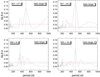 |
Fig. 5. GLS periodograms (cf. Sect. 3.2) in the data ranges of Table 5 showing the presence of the long cycle. Horizontal lines show, from top to bottom, the false alarm probability at the 1%, 5%, and 10% levels. |
Time ranges used to search for the second periodicity Pl.
3.3. Changes in the shape of the orbital light curve
We constructed orbital light curves for the seven datasets using the periods reported in Table 5. We find the following morphological changes in the orbital light curve (Fig. 6): (i) the relative depth of the main and secondary eclipse change, (ii) sometimes the secondary eclipse practically disappears in the first dataset, and (iii) the scatter is larger outside the main eclipse and larger in the last dataset. We find that part of the observed scatter in the light curves is due to the long-cycle variability; this can be observed in the relative coherence of colored data strings. However, the color step in the last datasets (on the order of the long cycle) and the presence of scatter (even through different color segments) shows that time variability is not limited to orbital and long-cycle timescales; however, we detect variations at even longer timescales. An analysis of the temporal distance between adjacent data points of all V-band data shows that the variability has a larger amplitude on timescales longer than about 1 day (Fig. 7).
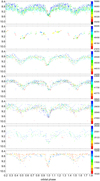 |
Fig. 6. Light curves phased with the periods reported in Table 5 for HJD′ ranges (color-coded, see color scale at right). The vertical axes are V-band magnitudes. The typical error for a single data point is 0.01 mag. |
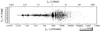 |
Fig. 7. Temporal distance between adjacent data points of all V-band data plotted against the corresponding difference in magnitude. We find that increased variability amplitude is observed on timescales longer than about 1 day. |
3.4. Infrared colors
The WISE mean magnitudes of RX Cas are W1 = 5.46121 ± 0.14338 mag, W2 = 5.16893 ± 0.17755, W3 = 5.04393 ± 0.15649 mag, and W4 = 4.68714 ± 0.14529 mag, based on 14 measurements obtained between MJD = 55246.60218 and 55249.97651. The colors are W1 − W2 = 0.292 mag and W2 − W3 = 0.125 mag.
We compared these infrared colors with those of double periodic variables (DPVs) and Be stars. The DPVs are close binaries that mostly consist of a B-type hotter star surrounded by an accretion disk fed by Roche-lobe overflow and mass transfer from a cooler giant companion (Mennickent 2017, 2022). Be stars are rapidly rotating B-type stars surrounded by a circumstellar disk. Both types of objects usually show a color excess that is mostly attributed to circumstellar reddening; therefore, they are used here to compare the presence of circumstellar matter. No correction for interstellar reddening was performed. However, at these wavelengths, the effect of interstellar reddening is negligible. In addition, we included as a reference the average colors for 136 main sequence stars in the range of spectral types from B1 V to K3 V from the HIPPARCOS catalog (Perryman et al. 1997). Further details regarding the data selection of DPVs, Be stars, and HIPPARCOS stars are available in Mennickent et al. (2016). The system appears in the W1 − W2 versus W2 − W3 diagram in an area populated by systems with color excess and circumstellar envelopes, far from the place where the HIPPARCOS nonvariable stars are located (Fig. 8). This finding suggests that circumstellar matter is present in RX Cas. The same tendency is found when comparing the published 2MASS JHK magnitudes 6.243 ± 0.018, 5.618 ± 0.036, and 5.435 ± 0.018 (Skrutskie et al. 2006), yielding J − H (0.625 ± 0.040) versus H − K (0.183 ± 0.040) colors, with those of synthetic models for dwarfs and giants, along with observed colors of Be stars and DPVs (Fig. 9). The RX Cas system is located far from the loci occupied by dwarfs and giants, suggesting the existence of circumstellar matter.
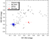 |
Fig. 8. Color-color diagram for nonvariable HIPPARCOS stars of spectral type B1 V - K3 V, Be stars, DPVs according to Mennickent et al. (2016) and RX Cas (this paper). |
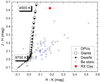 |
Fig. 9. Colors for Galactic DPVs (Mennickent et al. 2016), Be stars (Howells et al. 2001), and synthetic stellar atmosphere models with log g = 4.0 (squares with lines) and log g = 3.0 (open circles with lines) from Bessell et al. (1998). The effective temperature of two selected synthetic models have been labeled along with the position of RX Cas. |
4. Light curve model
An optimized simplex algorithm was used to solve the inverse problem adjusting the light curve with the best stellar-orbital-disk parameters for the system. The basic elements of the model, together with the light curve synthesis procedure, can be found in the literature (Djurašević 1992a, 1996) along with new and improved versions (Djurašević et al. 2008), which have been applied to several close binaries in the past (e.g., Mennickent & Djurašević 2013; Rosales et al. 2018; Mennickent et al. 2020). The model describes the total flux of the binary as the sum of the stellar fluxes and the radiation emerging from an optically thick accretion disk surrounding the hotter star and includes the geometrical effects produced by the observer inclination. This is an idealized representation of the binary system and its circumstellar environment; it does not consider possible mass outflows, gas streams, winds, or jets. However, based on our previous experience, it reproduces well the main physical structures contributing to the overall light curve in a binary of this type, and it is able to reproduce the orbital light curve reasonably well, as we show later in this work.
We considered some of the stellar and system parameters as fixed (Andersen et al. 1989), allowing the parameters of the disk to vary. The disk is characterized by its radius Rd, the vertical thickness at the central and outer edge (dc and de, respectively), and a radial dependent temperature profile
 (4)
(4)
where Td is the disk temperature at its outer edge (r = Rd) and aT is the temperature exponent (aT ≤ 0.75). The value of the exponent aT shows how close the radial temperature profile is to the steady-state configuration (aT = 0.75). In addition, the model considers two shock regions in the disk edge. One is the hot spot located around the hypothetical impact point between the gas stream ejected from the inner Lagrangian point and the disk, and the other is a bright spot located somewhere in the disk edge. Both represent regions in the disk with variable thickness and temperatures with respect to the surrounding disk; they have been detected in Doppler maps of Algols and also in hydrodynamical simulations of gas flows in close binary stars (e.g., Albright & Richards 1996; Bisikalo et al. 2000; Atwood-Stone et al. 2012).
In our model the two regions are characterized by their relative temperatures Ahs ≡ Ths/Td and Abs ≡ Tbs/Td, their angular dimensions θhs and θbs, and their angular locations measured from the line joining the stars in the direction of the orbital motion λhs and λbs. Finally, θrad is the angle between the line perpendicular to the local disk edge surface and the direction of the hot spot maximum radiation. We also consider the parameter Fd ≡ Rd/Ryk as a measure of the disk radius, where Ryk is defined by Djurašević (1992a) as the distance between the center of the hot star and its Roche lobe in the direction perpendicular to the line joining the star centers. Defined in this way, the disk is only stable within the limit Fd ≤ 1, while with a larger disk radius the material outside the Roche oval would go to the surrounding space and most likely in the area of the Lagrange equilibrium point L3, escaping from the system and forming a kind of circumbinary envelope.
Some parameters in the final analysis are fixed on the basis of averaged solutions obtained by analyzing all light curves on all strings and considering the published stellar and system parameters. These parameters are not expected to change during the analyzed period, so variations of disk parameters over time could be clearly distinguished as a consequence of the variable rate of accretion from the donor to the disk around the gainer. These parameters include the orbital inclination i = 81 1, the gravitational darkening coefficients βg = 0.25, βd = 0.08 and the albedo components Ag = 1.0 and Ad = 0.5, taken in the classical way on the basis of theoretical predictions for stars of given spectral types in radiation (gainer) and convective (donor) equilibrium. After some trials, we decided to keep fixed the nonsynchronous rotation coefficient of the gainer at fg ≡ Porb/Prot = 40 in order to best match the evolutionary tracks discussed in Sect. 5. This fg implies a rather slow rotation and an equivalent radius of 5.3 R⊙, contrary to the value of 2.8 R⊙ obtained with critical rotation using fg = 120. However, we note that similar good fits are obtained with gainer radii from 3 to 5 R⊙, so this fg parameter is not well constrained in our study. Other fixed parameters are the mass ratio q = Md/Mg = 0.31, Tg = 15 200 K and Td = 4580 K, as well as the filling factor for the critical Roche lobe of the donor Fd = 1.0 and the nonsynchronous rotation coefficients of the donor fd = 1.00. We also considered fixed Mg = 5.8 M⊙, Md = 1.8 M⊙, Rh = 2.57 R⊙, Rd = 23.73 R⊙, log gh, c = 4.38 ; 1.94,
  = −1.46; −1.08, Ωg, d = 40.241 ; 2.488, these last are the dimensionless surface potentials of the gainer and donor, respectively. Finally, we considered an orbital semimajor axis aorb = 83.92 R⊙. Most of these figures are consistent with the published stellar and orbital parameters by Andersen et al. (1989).
We performed the fit to the light curve at the data strings characterized in Table 5. The strings were divided in order to represent different sections of the long cycle. The epoch of maximum brightness of the long cycle was chosen as phase Φl = 0. Due to intrinsic variability, time lags, and the noise of the datasets, it was impossible to obtain light curves clear enough to get fits for every portion of the long cycle. We had to merge certain light curves to improve definition. We assume a symmetrical behavior of the orbital light curve during the first and second half-cycle of the long cycle. This is a strong assumption, but is the only one that allowed us to perform the fits that cover the orbital phases well, and as we show later, produce consistent results at the different strings so it can be justified a posteriori.
The results of the light curve fits are shown in Figs. 10 and 11, illustrating the uncertainties of measurements, typical orbital variability, long-term variability, and fit quality. Views of the system at different orbital phases are illustrated in Fig. 12. The results of the models are given in Table 6. The errors of the parameters were estimated by numerical experiments around the best global solution. Some correlations between the parameters can be observed (Figs. 13–16). The following conclusions can be drawn: (i) the long-cycle light curve, except for string 3, shows, as expected, a brighter magnitude at maximum (Φl = 0.0) and a decrease in brightness toward the minimum; (ii) the disk temperature at the outer edge decreases when the disk radius increases; (iii) the aT index increases as the disk radius increases; (iv) the disk radius decreases from long-cycle maximum to long-cycle minimum; and (v) the vertical thickness of the disk at the outer edge decreases from long-cycle maximum to long-cycle minimum, whereas the vertical thickness at the inner edge slightly increases.
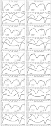 |
Fig. 10. Light curves, model prediction, and relative flux contribution at V band for donor, disk, and gainer, for five data segments in strings 3 (left) and 4 (right). The long-cycle phases 0.0, 0.15, 0.25, 0.35, and 0.50 are represented in the panels labeled max, mid1, mid2, mid3, and min, respectively. The typical error for a single data point is 0.01 mag. |
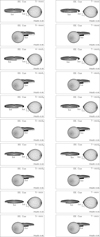 |
Fig. 12. Views of the system at orbital phases 0.20 and 0.95 derived from data of strings 5 (left) and 7 (right). From top to bottom the long-cycle phases 0.0, 0.15, 0.25, 0.35, and 0.50 are represented. |
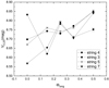 |
Fig. 13. V-band magnitude at orbital phase 0.25 for different data strings. The estimated error is given as illustration for one data point. |
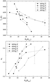 |
Fig. 14. Disk temperature vs. disk radius (top) and aT coefficient vs. disk radius (bottom) for different data strings. The estimated error is given as illustration for one data point. |
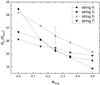 |
Fig. 15. Disk radius as a function of the long-cycle phase. The estimated error is given as illustration for one data point. |
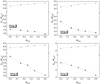 |
Fig. 16. Disk outer (dot) and inner (asterisk) edge thickness vs. long-cycle phase for different data strings. Estimated errors are given as illustration for some data points. |
Model data for light curves of different string numbers (#) at selected long-cycle phases (Φl).
In addition, regarding the variability of the parameters as measured by their standard deviation, we can say the following: (i) the position of the bright spot is 25 times more variable than the position of the hot spot; (ii) De variability is 10 times that of Dc; (iii) the most variable parameter is θrad (700 %); and (iv) the disk radius varies at the level of 3% and its temperature 5%.
5. Evolutionary stage
For the calculation of the evolution of the possible RX Cas progenitor binary system, the Modules for Experiments in Stellar Astrophysics (MESA) code (Paxton et al. 2011, 2013, 2015, 2018) was used, in revision 10398. This code simultaneously calculates the detailed evolution of both stars within each binary system. Since it is expected that close systems circularize with time due to tidal effects (Zahn 1977), especially when they evolve to fill their Roche lobes (Verbunt & Phinney 1995), the binary systems are assumed to have circular orbits. The mass transfer rate is calculated according to the Ritter scheme (Ritter 1988). The composition of accreted material is identical to the donor’s current surface composition. Binary systems lose mass and angular momentum due to the stellar wind mass loss and nonconservative mass transfer. The stellar wind mass loss rate of each star is calculated according to the so-called “Dutch” option in the MESA code (Vink et al. 2001) and the metallicity was set to 0.02. The matter lost due to the stellar wind has the specific orbital angular momentum of its star. Considering an angular momentum loss due to nonconservative mass transfer, it follows Soberman et al. (1997), where the fixed fraction of the transferred mass (β) is lost isotropically from the secondary star.
After some numerical experiments we find that there are two evolutionary routes that reproduce the observed properties of RX Cas, both via Case B mass transfer evolution. The first is conservative or almost conservative evolution and the second is highly nonconservative evolution with accretion efficiency of only 10% (β = 0.1). In the conservative or nearly conservative evolution we show two cases. Both cases are illustrated in evolutionary tracks in the luminosity–temperature diagrams in Fig. 17 and are summarized in Table 7.
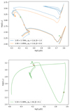 |
Fig. 17. Evolutionary tracks for the models described in Table 5. Upper plot: the donors (circles) and gainers (diamonds) are shown in the same colors as the evolutionary lines (see legend in inset), whereas the observed values are shown in green. Lower plot: the modeled values are again in the same color as the evolutionary line and the observed values are in red. The initial masses and periods, along with the accretion efficiency, are shown for the models. |
Modeled and observed parameters for RX Cas.
In the first conservative case, the initial system of 3.95 + 3.70 M⊙ stars and with orbital period of 11 days enters conservative Case B mass transfer after 1.5313 × 10⁸ years. At that moment, the primary has completed its hydrogen core burning phase and the secondary is still a main sequence star with a central hydrogen abundance fraction of 0.17. At the time the orbital period of this system reaches the observed value (32 324), the mass of the primary star (donor) is 1.72 M⊙ and the mass of the secondary star (gainer) is 5.92 M⊙. Their effective temperatures are 4400 K and 19 000 K and radii are 23.5 R⊙ and 3.80 R⊙, respectively. The mass transfer rate at this moment is 8.0 × 10⁻⁶ M⊙ yr−1. This binary system evolves further to the end of Case B mass transfer (at 1.5436 × 10⁸ yr) and at that time the primary is a helium core burning star of 0.84 M⊙ and the secondary is a rejuvenated main sequence star of 6.80 M⊙ with the central hydrogen abundance of 0.49. The orbital period of this system is 182.9 days.
In the second almost conservative case, the initial binary of 3.90 + 3.85 M⊙ stars and orbital period of 11 days is followed through a Case B evolution with an assumed accretion efficiency of 90%. Mass transfer starts at 1.5826 × 10⁸ yr, when the primary has completed its hydrogen core burning phase and its envelope starts expanding. The secondary star is at the end of this phase as well, with the central hydrogen abundance fraction of only 0.004. When the orbital period reaches a value of 32.324 days, the donor is a 1.77 M⊙ star with an effective temperature of 4400 K and a radius of 23.8 R⊙. At the same time, the gainer is a 5.76 M⊙ star with Teff = 17 900 K and R = 4.0 R⊙. The mass transfer rate is about 5 × 10⁻⁶ M⊙ yr−1. At the end of Case B mass transfer, the primary is a 0.89 M⊙ star and the secondary is a 6.56 M⊙ star in an orbit with a 171.4-day period.
For the case of nonconservative evolution, which assumes a significant mass loss from the system, the initial masses have to be higher: 5.5 + 5.4 M⊙. The initial orbital period is 4 days. This system enters Case B mass transfer at 6.7278 × 10⁸ yr. The primary has completed core hydrogen burning and the fraction of secondary central hydrogen abundance is 0.04. When the orbital period reaches the observed value, the masses of donor and gainer are 1.80 M⊙ and 5.76 M⊙, respectively. Their effective temperatures are 4570 K and 16 300 K and radii are 23.9 R⊙ and 5.2 R⊙. The mass transfer rate is about 4 × 10⁻⁵ M⊙ yr−1. At the end of Case B mass transfer, the masses of the stellar components are 0.83 M⊙ and 5.86 M⊙ and the orbital period is 253.6 days. The primary is a core helium burning star and the secondary is a rejuvenated main sequence star with a fraction of central hydrogen abundance of 0.25. From the above calculations, we find that the model that best matches the MESA tracks is the nonconservative model.
In all systems, after a while, the secondary star will also ignite helium in its core. Due to the higher mass, the secondary star will complete helium core burning before the primary. The next mass transfer, from the secondary to the primary star, will take place due to the secondary envelope expansion and will likely result in a common envelope and a possible merger, considering that the mass ratio of the stellar components is far from unity.
A review of the parameters of RX Cas reported in the literature reveals the large spread in some parameters and the problems generated by not properly including the accretion disk in the system geometry or the line blending in spectroscopic data (Table 8).
Summary of parameters of RX Cas reported in the literature.
6. Discussion
The high-excitation emission lines observed in the ultraviolet region in this and other similar systems have been interpreted in terms of a high-temperature wind induced by the accretion process emanating from the disk–gainer interface or from a disk chromosphere (Fig. 18; Plavec & Koch 1978; Weiland & Plavec 1983; Plavec 1992). This is consistent with the cooling of this wind at larger distances and the interpretation of the excess in the L and M bands in terms of emission from a circumbinary shell of luminosity 3 × 1033 erg and mass 1 × 10²³ g of radius 4.6 × 1014 cm (i.e., 70 times the orbital separation; Taranova & Shenavrin 1997). This is consistent with the infrared excess we found in JHK and WISE photometry colors. The existence of hot plasma around the gainer is also consistent with the greater depth of the main eclipse at the U band (Kříž et al. 1980).
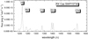 |
Fig. 18. Spectrum labeled SWP15730 obtained from the database of the satellite International Ultraviolet Explorer showing emission lines in some high excitation lines. |
The expected period change in the conservative case is (Huang 1963)
 (5)
(5)
Using these numbers and the derived stellar masses, we determine Ṁc = 6.45 × 10⁻⁶ M⊙ yr−1. This figure is consistent with the value found by Andersen et al. (1989) of ∼6 × 10⁻⁶ M⊙ yr−1. However, we find that nonconservative evolution is also possible, and in this case the mass transfer rate derived previously would not be valid.
RX Cas is part of a group of interacting binaries showing light curves similar to β Lyrae and showing a long photometric cycle of unknown origin (Mennickent 2017). Few of these interacting binaries have been studied in terms of their physical changes during the long cycle. Here we provide a brief comparison with some of them. In RX Cas, we find that the long cycle of around 516 days can be explained in terms of changes of the physical parameters of the accretion disk, which was mentioned along with other possible causes in the past (Kříž et al. 1980). The disk turns out to be hotter and thicker at long-cycle maximum, but it does not change appreciably in radial extension. We note that a hotter disk during maximum was predicted by a simpler study in the past (Djurašević 1993). Contrarily, large changes in disk radius and thickness have been inferred in OGLE-BLG-ECL-157529, a binary characterized by orbital and long periods of 24 8 and ∼850 days, while its long cycle can be reproduced by occultation of the gainer by a variable disk thickness (Mennickent & Djurašević 2021). On the other hand, the system OGLE-LMC-DPV-097 is characterized by a long-cycle length of ∼306 days and an amplitude of ∼0.8 mag in the I band. This binary has an orbital period of 7
 75 and relatively low stellar masses of 5.5 and 1.1 M⊙. In this system the orbital light curve changes in a systematic way during the long cycle. At the minimum of the long cycle the secondary eclipse practically disappears and during the ascending branch the system is brighter in the first quadrant than during the second quadrant. The disk radius is 7.5 R⊙ at the minimum and 15.3 R⊙ at the ascending branch of the long cycle; its temperature at the outer edge changes from 6870 to 4030 K in these two stages (Garcés et al. 2018). OGLE-LMC-DPV-065 is another interesting binary with a large amplitude of the long cycle. The long cycle is characterized by a double hump light curve in the I and V bands whose general shape is nearly constant with only minor variations. After a continuous decrease in the long-period from 350 to 218 d lasting about 13 yr, the long cycle remained almost constant for about 10 yr. However, the orbital light curve is fairly constant in shape, and no clear link between the disk structure and long cycle has been observed for this system, in a clear contrast to OGLE-LMC-DPV-097 and RX Cas (Mennickent et al. 2019). From the above we conclude that we cannot draw general conclusions about disk changes and photometric long cycles in these few systems as they show different behaviors that cannot be easily adapted to a global single picture.
However, it is highly probable that these changes are driven by variable rates of accretion, and the existence of a cycle of hundreds of days might indicate some mechanism controlling periodically (or semiperiodically) the amount of mass transferred from the donor. It is worth mentioning the possibility of a magnetic dynamo, where the Applegate mechanism and the effect on the quadrupole gravitational momentum (and shape) of the donor plays a role since it should regulate the mass transferred through the inner Lagrangian point (Schleicher & Mennickent 2017). In the framework of the simple dynamo model proposed by these authors, RX Cas should have a long cycle that is 40% longer than the observed one. The dynamo might not control only the mass transfer rate, but also, indirectly, the properties of the accretion disk. To date, not enough observations have been conducted to determine whether magnetic activity is present in this binary.
7. Conclusions
Our study contributes to the understanding of this relatively well-studied semidetached close interacting binary: for the first time we have modeled the orbital light curve at different stages of the long photometric cycle. Few similar systems have been studied and modeled in detail at different long-cycle phases. Since the nature of this cycle is still unknown, highlights can be obtained from this process, especially considering that records of 109 years of photometry of RX Cas are studied in our work. Due to large data gaps and the long-term photometric variability, for our analysis we had to assume that the system properties are symmetrical regarding the long cycle; in other words, the same properties in the first half of the long cycle as in the second half, with similar properties at phases 0.25 and 0.75 and at 0.4 and 0.6, for instance. This is a limitation of our analysis, along with the (generally accepted) assumption of disk geometry for the circumstellar envelope. However, these assumptions allowed us to get important new insights on the long cycle and its relationship with the accretion disk.
We find changes in the shape of the orbital light curve of RX Cas during the long cycle. With a simple model including the stellar and disk flux contributions we find that these changes can be interpreted in terms of variability of the parameters of the optically thick disk surrounding the hotter star. We speculate that these changes can be induced by variable mass transfer from the donor. The epochs of maximum brightness are those with thicker and hotter disks, while the disk radius practically does not change, suggesting that the system brightness is controlled by the disk brightness, which is not the case of OGLE-BLG-ECL-157529, where its long cycle can be reproduced by occultation of the gainer by a variable disk thickness (Mennickent & Djurašević 2021). In both cases, however, a variable mass transfer rate might be controlling the relative flux contributions of gainer, donor, and disk and introduce additional occultation effects. Although the 1D binary star evolutionary code MESA was used to find possible evolutionary routes and progenitors for this system, a unique solution was not found, especially due to the uncertainty of the impact of nonconservative mass transfer processes and the unknown rotational velocity of the gainer. Our multiparametric light curve model is sensible to small fluctuations in some parameters providing similar solutions still compatible with the observed data and their errors. However, these variations are relatively minor and the general trends observed in the analyzed datasets give confidence of the used methodology. The nonconservative evolution is a real possibility for this system since a circumbinary dust shell has been reported from infrared photometric studies. We obtain a good match of the system’s current parameters with a highly nonconservative evolution, although the presence of a disk is not considered in the mass loss processes included in the MESA evolutionary tracks. Since a magnetic dynamo operating in the donor star has been proposed as the cause of the long cycle, it would be desirable to pursue future polarimetric observations aimed to detect signatures of magnetic fields in the cooler stellar component.
Acknowledgments
We thank the referee Dr. Petr Harmanec who provided comments and suggestions that helped to improve the first version of this manuscript. R.E.M. and D.S. gratefully acknowledge support by the ANID BASAL projects ACE210002 and FB210003, FONDECYT Regular 1190621 and FONDECYT Regular 1201280. G. D., I. V., J. P. and M. I. J. acknowledge the financial support of the Ministry of Education, Science and Technological Development of the Republic of Serbia through the contract No 451-03-68/2020/14/20002. This research has made use of: (1) the SIMBAD database, operated at CDS, Strasbourg, France (Wenger et al. 2000), (2) data products from the Wide-field Infrared Survey Explorer, which is a joint project of the University of California, Los Angeles, and the Jet Propulsion Laboratory/California Institute of Technology, funded by the National Aeronautics and Space Administration, (3) the NASA/ IPAC Infrared Science Archive, which is operated by the Jet Propulsion Laboratory, California Institute of Technology, under contract with the National Aeronautics and Space Administration, (4) data products from the Two Micron All Sky Survey, which is a joint project of the University of Massachusetts and the Infrared Processing and Analysis Center/California Institute of Technology, funded by the National Aeronautics and Space Administration and the National Science Foundation and (5) data from the OMC Archive at CAB (INTA-CSIC), pre-processed by ISDC.
References
- Albright, G. E., & Richards, M. T. 1996, ApJ, 459, L99 [NASA ADS] [Google Scholar]
- Alduseva, V. Y. 1987, Sov. Astron., 31, 310 [NASA ADS] [Google Scholar]
- Andersen, J., Pavlovski, K., & Piirola, V. 1989, A&A, 215, 272 [NASA ADS] [Google Scholar]
- Atwood-Stone, C., Miller, B. P., Richards, M. T., Budaj, J., & Peters, G. J. 2012, ApJ, 760, 134 [NASA ADS] [CrossRef] [Google Scholar]
- Bessell, M. S., Castelli, F., & Plez, B. 1998, A&A, 333, 231 [NASA ADS] [Google Scholar]
- Brancewicz, H. K., & Dworak, T. Z. 1980, AcA, 30, 501 [NASA ADS] [Google Scholar]
- Bisikalo, D. V., Harmanec, P., Boyarchuk, A. A., Kuznetsov, O. A., & Hadrava, P. 2000, A&A, 353, 1009 [NASA ADS] [Google Scholar]
- Blažko, S. 1906, Astron. Nachr., 172, 57 [Google Scholar]
- Ceraski, W. 1904, Astron. Nachr., 164, 217 [Google Scholar]
- Crawford, J. A. 1955, ApJ, 121, 71 [NASA ADS] [CrossRef] [Google Scholar]
- Deschamps, R., Braun, K., Jorissen, A., et al. 2015, A&A, 577, A55 [NASA ADS] [CrossRef] [EDP Sciences] [Google Scholar]
- Djurašević, G. 1992a, Ap&SS, 196, 267 [Google Scholar]
- Djurašević, G. 1993, Ap&SS, 206, 129 [CrossRef] [Google Scholar]
- Djurašević, G. 1996, Ap&SS, 240, 317 [Google Scholar]
- Djurašević, G., Vince, I., & Atanacković, O. 2008, AJ, 136, 767 [Google Scholar]
- Eggleton, P. 2006, Evolutionary Processes in Binary and Multiple Stars (Cambridge University Press) [Google Scholar]
- Eggleton, P. P., & Kisseleva-Eggleton, L. 2006, Ap&SS, 304, 75 [NASA ADS] [CrossRef] [Google Scholar]
- Gaposchkin, S. 1944, AJ, 51, 66 [NASA ADS] [CrossRef] [Google Scholar]
- Gaposchkin, S. 1944, ApJ, 100, 230 [NASA ADS] [CrossRef] [Google Scholar]
- Garcés, L. J., Mennickent, R. E., Djurašević, G., Poleski, R., & Soszyński, I. 2018, MNRAS, 477, L11 [CrossRef] [Google Scholar]
- Gies, D. R. 2007, ASP Conf. Ser., 367, 325 [NASA ADS] [Google Scholar]
- Domingo, A., Gutiérrez-Sánchez, R., Rísquez, D., et al. 2010, Astrophys. Space Sci. Proc., 14, 493 [NASA ADS] [CrossRef] [Google Scholar]
- Haas, J. 1924, Astron. Nachr., 220, 337 [Google Scholar]
- Harmanec, P. 1998, A&A, 335, 173 [NASA ADS] [Google Scholar]
- Howells, L., Steele, I. A., Porter, J. M., & Etherton, J. 2001, A&A, 369, 99 [NASA ADS] [CrossRef] [EDP Sciences] [Google Scholar]
- Huang, S.-S. 1963, ApJ, 138, 471 [NASA ADS] [CrossRef] [Google Scholar]
- Hubeny, I., Harmanec, P., & Shore, S. N. 1994, A&A, 289, 411 [NASA ADS] [Google Scholar]
- Kafka, S. 2021, Observations from the AAVSO International Database [Google Scholar]
- Kalv, P. 1979, TarOT, 58, 3 [NASA ADS] [Google Scholar]
- Kippenhahn, R., & Weigert, A. 1967, Z. Astrophys., 65, 251 [NASA ADS] [Google Scholar]
- Kochanek, C. S., Shappee, B. J., Stanek, K. Z., et al. 2017, PASP, 129, 104502 [Google Scholar]
- Kopal, Z. 1959, Close Binary Stars (New York: Wiley) [Google Scholar]
- Kreiner, J. M. 1978, IBVS, 1403, 1 [NASA ADS] [Google Scholar]
- Kříž, S., Arsenijevič, J., Grygar, J., et al. 1980, Bull. Astron. Inst. Cz., 31, 284 [Google Scholar]
- Lenz, P., & Breger, M. 2005, Commun. Asteroseismol., 146, 53 [Google Scholar]
- Lubow, S. H., & Shu, F. H. 1975, ApJ, 198, 383 [NASA ADS] [CrossRef] [Google Scholar]
- Maehara, H. 2014, JAXA Research and Development Report, 13, 119 [Google Scholar]
- Martynov, D. Y. 1950, Bull. Astron., Obs. Engelhardt, 27, 3 [Google Scholar]
- Martynov, D. Y., Zajtseva, G. V., & Kumsiashvili, M. I. 1980, PZ, 21, 451 [NASA ADS] [Google Scholar]
- Martynov, D. Y., Kumsiashvili, M. I., Voloshina, I. B., Zajtseva, G. V., & Todorova, P. N. 1987, PZ, 22, 561 [NASA ADS] [Google Scholar]
- Mas-Hesse, J. M., Giménez, A., Culhane, J. L., et al. 2003, A&A, 411, L261 [NASA ADS] [CrossRef] [EDP Sciences] [Google Scholar]
- Mennickent, R. E. 2017, Serb. Astron. J., 194, 1 [NASA ADS] [CrossRef] [Google Scholar]
- Mennickent, R. E. 2022, Galax, 10, 15 [NASA ADS] [CrossRef] [Google Scholar]
- Mennickent, R. E., & Djurašević, G. 2013, MNRAS, 432, 799 [NASA ADS] [CrossRef] [Google Scholar]
- Mennickent, R. E., Otero, S., & Kołaczkowski, Z. 2016, MNRAS, 455, 1728 [NASA ADS] [CrossRef] [Google Scholar]
- Mennickent, R. E., Cabezas, M., Djurašević, G., et al. 2019, MNRAS, 487, 4169 [NASA ADS] [CrossRef] [Google Scholar]
- Mennickent, R. E., Djurašević, G., Vince, I., et al. 2020, A&A, 642, A211 [NASA ADS] [CrossRef] [EDP Sciences] [Google Scholar]
- Mennickent, R. E., & Djurašević, G. 2021, A&A, 653, A89 [NASA ADS] [CrossRef] [EDP Sciences] [Google Scholar]
- Paxton, B., Bildsten, L., Dotter, A., et al. 2011, ApJS, 192, 3 [Google Scholar]
- Paxton, B., Cantiello, M., Arras, P., et al. 2013, ApJS, 208, 4 [Google Scholar]
- Paxton, B., Marchant, P., Schwab, J., et al. 2015, ApJS, 220, 15 [Google Scholar]
- Paxton, B., Schwab, J., Bauer, E. B., et al. 2018, ApJS, 234, 34 [NASA ADS] [CrossRef] [Google Scholar]
- Perryman, M. A. C., Lindegren, L., Kovalevsky, J., et al. 1997, A&A, 323, L49 [Google Scholar]
- Plavec, M. J. 1980, IAUS, 88, 251 [NASA ADS] [Google Scholar]
- Plavec, M. J. 1992, ASP Conf. Ser., 22, 47 [NASA ADS] [Google Scholar]
- Plavec, M., & Koch, R. H. 1978, IBVS, 1482, 1 [NASA ADS] [Google Scholar]
- Pourbaix, D. 2019, MmSAI, 90, 318 [NASA ADS] [Google Scholar]
- Pols, O. R., Cote, J., Waters, L. B. F. M., et al. 1991, A&A, 241, 419 [NASA ADS] [Google Scholar]
- Pustylnik, I., Kalv, P., & Harvig, V. 2007, Astron. Astrophy. Trans., 26, 31 [NASA ADS] [CrossRef] [Google Scholar]
- Roche, M. 1873, Mem. Acad. Sci. Montpellier, 8, 235 [Google Scholar]
- Ritter, H. 1988, A&A, 202, 93 [NASA ADS] [Google Scholar]
- Rosales, J. A., R. E., Mennickent G., Djurašević et al. 2018, MNRAS, 476, 3039 [NASA ADS] [CrossRef] [Google Scholar]
- Scargle, J. D. 1982, ApJ, 263, 835 [Google Scholar]
- Schleicher, D. R. G., & Mennickent, R. E. 2017, A&A, 602, A109 [NASA ADS] [CrossRef] [EDP Sciences] [Google Scholar]
- Shappee, B. J., Prieto, J. L., Grupe, D., et al. 2014, ApJ, 788, 48 [Google Scholar]
- Skrutskie, M. F., Cutri, R. M., Stiening, R., et al. 2006, AJ, 131, 1163 [NASA ADS] [CrossRef] [Google Scholar]
- Soberman, G. E., Phinney, E. S., & van den Heuvel, E. P. J. 1997, A&A, 327, 620 [NASA ADS] [Google Scholar]
- Stellingwerf, R. F. 1978, ApJ, 224, 953 [Google Scholar]
- Sterken, C. 2005, ASPC, 3, 335 [Google Scholar]
- Strupat, W. 1987, A&A, 185, 150 [NASA ADS] [Google Scholar]
- Struve, O. 1944, ApJ, 99, 295 [NASA ADS] [CrossRef] [Google Scholar]
- Taranova, O. G., & Shenavrin, V. I. 1997, Astron. Lett., 23, 698 [NASA ADS] [Google Scholar]
- Verbunt, F., & Phinney, E. S. 1995, A&A, 296, 709 [NASA ADS] [Google Scholar]
- Vink, J. S., de Koter, A., & Lamers, H. J. G. L. M. 2001, A&A, 369, 574 [NASA ADS] [CrossRef] [EDP Sciences] [Google Scholar]
- Wendell, O. C. 1913, AnHar, 69, 99 [NASA ADS] [Google Scholar]
- Wenger, M., Ochsenbein, F., Egret, D., et al. 2000, A&A, 143, 9 [NASA ADS] [Google Scholar]
- Weiland, J. L., & Plavec, M. J. 1983, BAAS, 15, 916 [NASA ADS] [Google Scholar]
- Wilson, R. E. 2018, ApJ, 869, 19 [CrossRef] [Google Scholar]
- Wright, E. L., Eisenhardt, P. R. M., Mainzer, A. K., et al. 2010, AJ, 140, 1868 [Google Scholar]
- Zahn, J.-P. 1977, A&A, 57, 383 [NASA ADS] [Google Scholar]
- Zechmeister, M., & Kürster, M. 2009, A&A, 496, 577 [CrossRef] [EDP Sciences] [Google Scholar]
All Tables
Model data for light curves of different string numbers (#) at selected long-cycle phases (Φl).
All Figures
|
Fig. 1. V magnitudes from the datasets listed in Table 1 during the whole range of observing dates. Data distributions and their fits are shown on the right side. The typical error for a single data point is 0.01 mag. |
| In the text | |
|
Fig. 2. Close-up of V magnitudes from the datasets listed in Table 1 during selected ranges of observing dates. The typical error for a single data point is 0.01 magnitude. |
| In the text | |
|
Fig. 3. Magnitudes from the KWS-I and ASAS-SN V and g datasets. The typical error for a single data point is 0.01 magnitude. |
| In the text | |
|
Fig. 4. Observed minus calculated times of minima, normalized to the test period Po = 32 |
| In the text | |
|
Fig. 5. GLS periodograms (cf. Sect. 3.2) in the data ranges of Table 5 showing the presence of the long cycle. Horizontal lines show, from top to bottom, the false alarm probability at the 1%, 5%, and 10% levels. |
| In the text | |
|
Fig. 6. Light curves phased with the periods reported in Table 5 for HJD′ ranges (color-coded, see color scale at right). The vertical axes are V-band magnitudes. The typical error for a single data point is 0.01 mag. |
| In the text | |
|
Fig. 7. Temporal distance between adjacent data points of all V-band data plotted against the corresponding difference in magnitude. We find that increased variability amplitude is observed on timescales longer than about 1 day. |
| In the text | |
|
Fig. 8. Color-color diagram for nonvariable HIPPARCOS stars of spectral type B1 V - K3 V, Be stars, DPVs according to Mennickent et al. (2016) and RX Cas (this paper). |
| In the text | |
|
Fig. 9. Colors for Galactic DPVs (Mennickent et al. 2016), Be stars (Howells et al. 2001), and synthetic stellar atmosphere models with log g = 4.0 (squares with lines) and log g = 3.0 (open circles with lines) from Bessell et al. (1998). The effective temperature of two selected synthetic models have been labeled along with the position of RX Cas. |
| In the text | |
|
Fig. 10. Light curves, model prediction, and relative flux contribution at V band for donor, disk, and gainer, for five data segments in strings 3 (left) and 4 (right). The long-cycle phases 0.0, 0.15, 0.25, 0.35, and 0.50 are represented in the panels labeled max, mid1, mid2, mid3, and min, respectively. The typical error for a single data point is 0.01 mag. |
| In the text | |
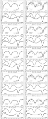 |
Fig. 11. Same as Fig. 10, but for strings 5 (left) and 7 (right). |
| In the text | |
|
Fig. 12. Views of the system at orbital phases 0.20 and 0.95 derived from data of strings 5 (left) and 7 (right). From top to bottom the long-cycle phases 0.0, 0.15, 0.25, 0.35, and 0.50 are represented. |
| In the text | |
|
Fig. 13. V-band magnitude at orbital phase 0.25 for different data strings. The estimated error is given as illustration for one data point. |
| In the text | |
|
Fig. 14. Disk temperature vs. disk radius (top) and aT coefficient vs. disk radius (bottom) for different data strings. The estimated error is given as illustration for one data point. |
| In the text | |
|
Fig. 15. Disk radius as a function of the long-cycle phase. The estimated error is given as illustration for one data point. |
| In the text | |
|
Fig. 16. Disk outer (dot) and inner (asterisk) edge thickness vs. long-cycle phase for different data strings. Estimated errors are given as illustration for some data points. |
| In the text | |
|
Fig. 17. Evolutionary tracks for the models described in Table 5. Upper plot: the donors (circles) and gainers (diamonds) are shown in the same colors as the evolutionary lines (see legend in inset), whereas the observed values are shown in green. Lower plot: the modeled values are again in the same color as the evolutionary line and the observed values are in red. The initial masses and periods, along with the accretion efficiency, are shown for the models. |
| In the text | |
|
Fig. 18. Spectrum labeled SWP15730 obtained from the database of the satellite International Ultraviolet Explorer showing emission lines in some high excitation lines. |
| In the text | |
Current usage metrics show cumulative count of Article Views (full-text article views including HTML views, PDF and ePub downloads, according to the available data) and Abstracts Views on Vision4Press platform.
Data correspond to usage on the plateform after 2015. The current usage metrics is available 48-96 hours after online publication and is updated daily on week days.
Initial download of the metrics may take a while.