| Issue |
A&A
Volume 693, January 2025
|
|
|---|---|---|
| Article Number | A112 | |
| Number of page(s) | 20 | |
| Section | Extragalactic astronomy | |
| DOI | https://doi.org/10.1051/0004-6361/202451702 | |
| Published online | 09 January 2025 | |
CASCO: Cosmological and AStrophysical parameters from Cosmological simulations and Observations
II. Constraining cosmology and astrophysical processes with early- and late-type galaxies
1
Dipartimento di Fisica “E. Pancini”, Università degli studi di Napoli Federico II, Compl. Univ. di Monte S. Angelo, Via Cintia, I-80126 Napoli, Italy
2
INAF – Osservatorio Astronomico di Capodimonte, Salita Moiariello 16, I-80131 Napoli, Italy
3
INFN, Sez. di Napoli, Compl. Univ. di Monte S. Angelo, Via Cintia, I-80126 Napoli, Italy
4
Kapteyn Astronomical Institute, University of Groningen, PO Box 800 9700 AV Groningen, The Netherlands
⋆ Corresponding authors; This email address is being protected from spambots. You need JavaScript enabled to view it.
; This email address is being protected from spambots. You need JavaScript enabled to view it.
Received:
29
July
2024
Accepted:
27
November
2024
Abstract
Physical processes can influence the formation and evolution of galaxies in diverse ways. It is essential to validate their incorporation into cosmological simulations by testing them against real data encompassing various types of galaxies and spanning a broad spectrum of masses and galaxy properties. For these reasons, in this second paper of the CASCO series, we compare the structural properties and dark matter content of early-type galaxies taken from the CAMELS IllustrisTNG cosmological simulations to three different observational datasets (SPIDER, ATLAS3D, and MaNGA DynPop), to constrain the value of cosmological and astrophysical feedback parameters, and we compare the results with those obtained comparing the simulation expectations with late-type galaxies. We consider the size-mass, internal DM fraction-mass, and internal DM mass-stellar mass relations for all the simulations, and search for the best-fit simulation for each set of observations. For SPIDER, we find values for the cosmological parameters in line with both the literature and the results obtained from the comparison between simulations and late-type galaxies; results for the supernovae feedback parameters are instead opposite with respect to the previous results based on late-type galaxies. For ATLAS3D, we find similar values as from SPIDER for the cosmological parameters, but we find values for the supernovae feedback parameters more in line with what we found for late-type galaxies. From MaNGA DynPop, we find extreme values for the cosmological parameters, while the supernovae feedback parameters are consistent with ATLAS3D results. When considering the full MaNGA DynPop sample, including both late- and early-type galaxies, no single simulation can reproduce the full variety in the observational datasets. The constraints depend strongly on the specific properties of each observational trend, making it difficult to find a simulation matching all galaxy types, indicating the existence of limitations in the ability of simulations in reproducing the observations.
Key words: methods: numerical / galaxies: evolution / galaxies: formation / dark matter
© The Authors 2025
 Open Access article, published by EDP Sciences, under the terms of the Creative Commons Attribution License (https://creativecommons.org/licenses/by/4.0), which permits unrestricted use, distribution, and reproduction in any medium, provided the original work is properly cited.
This article is published in open access under the Subscribe to Open model. This email address is being protected from spambots. You need JavaScript enabled to view it. to support open access publication.
1. Introduction
The study of galaxy formation and evolution is a cornerstone of modern astrophysics. One of the key challenges in this field is understanding the complex interplay between cosmology and astrophysical feedback mechanisms, and how they both shape the observable properties of galaxies.
In this regard, cosmological simulations constitute a useful tool for investigating this interplay. For example, the SEAGLE programme (Simulating EAGLE LEnses, Mukherjee et al. 2018, 2021, 2022) managed to constrain the stellar and AGN feedback processes that underlie the galaxy formation of massive lens galaxies by simulating and modelling strong lenses from the Evolution and Assembly of GaLaxies and their Environments (EAGLE) suite of cosmological simulations (Crain et al. 2015; Schaye et al. 2015). The programme obtained the projected dark matter (DM) fractions within half the effective radius and within the effective radius of simulated galaxies, showing good agreement with the Sloan Lens ACS Survey (SLACS; Bolton et al. 2006) lenses results. In recent years, cosmological simulation suites featuring thousands of different combinations of cosmological and astrophysical parameters have emerged, such as CAMELS (Villaescusa-Navarro et al. 2021, 2023; Ni et al. 2023). These suites are a powerful tool, in that they allow us to explore a wide range of parameter values, showing how cosmology and astrophysics influence the statistical properties of galaxies; it has been shown that one can infer information about cosmology and astrophysics even just from the physical properties of a single galaxy by training a machine learning model on simulated galaxies (Villaescusa-Navarro et al. 2022; Echeverri-Rojas et al. 2023) with an increased constraining potential when using the properties of multiple galaxies (Chawak et al. 2024). Other approaches that utilise CAMELS to infer cosmological parameters are the use of graph neural networks for field-level likelihood-free inference of Ωm with 12 per cent of precision (de Santi et al. 2023) and the inference of both Ωm and σ8 with galaxy photometry alone (Hahn et al. 2024). In the context of cosmological simulations, the work by Wu et al. (2024) shows that it is also possible to infer both total and dark matter mass within the effective radius of real galaxies by training a machine learning algorithm on photometry, sizes, stellar mass and kinematic features of simulated galaxies, with very high accuracy and almost no bias.
In this context, galaxy scaling relations, which are the relationships between different observable properties of galaxies, have been proven to be a useful tool for probing the effects of different astrophysical feedback processes (Tortora et al. 2019). In Busillo et al. (2023), hereafter referred to as Paper I, we developed a statistical method of determining, from a selection of CAMELS cosmological simulations with different values of cosmological and astrophysical parameters, which simulation’s set of galaxy scaling relations better fits the observed scaling relations for SPARC late-type galaxies (LTGs, Lelli et al. 2016).
In addition to gravity, cosmological simulations include various models for physical processes, such as supernovae and active galactic nucleus (AGN) feedback. These processes drive the conversion of gas into stars, and their efficiency is known to vary with mass (Dekel & Birnboim 2004; Tortora et al. 2019; Hunt et al. 2020). Furthermore, the distribution and the amount of dark matter and the expansion history of the Universe (summarised in the standard cosmological model) influences the distribution of the primordial dark matter seeds, the merger history of galaxies, and the mass assembly (Taylor & Rowan-Robinson 1992; Conselice et al. 2014). A comprehensive comparison of observed scaling relations involving stars and dark matter across a broad range of masses, galaxy types, and data samples with simulations is imperative. Therefore, in this Paper II the aim is to complement the analysis conducted in Paper I. We initially explore the scaling relations for massive early-type galaxies1 (ETGs) as a function of astrophysical and cosmological parameters. Subsequently, we compare these relations with observations, including in the analysis the scaling relations for LTGs. Our aim is to describe the dark matter content of galaxies across different galaxy types and a mass range of approximately three orders of magnitude in stellar mass.
The paper is structured as follows. In Section 2 we present both the simulated and observational datasets used in our analysis. In Section 3 we discuss some of the properties of the ETGs that we took from CAMELS for our analysis. We compare both the CAMELS simulations and the original IllustrisTNG simulations with the various observational datasets in Section 4, and state our conclusions in Section 5.
2. Data
In this section we introduce both the simulated and the observational datasets used for the analysis. We begin by describing the simulated dataset used, which includes data from both CAMELS and the original IllustrisTNG. We then describe the three main observational dataset used: SPIDER, ATLAS3D, and MaNGA DynPop. For each dataset we list the main observational quantities used for the analysis, and outline any filtering process operated on the raw datasets.
2.1. Simulated data
In the following, we provide a detailed description of the simulated datasets employed in our analysis. We first focus on the IllustrisTNG suite of CAMELS, detailing its main characteristics and the quantities that we chose to use in our analysis. Next, we describe the original simulation suites from the IllustrisTNG project, specifying what simulations have been considered for the analysis and the values of the cosmological parameters assumed in them.
2.1.1. CAMELS
Similarly to Paper I, we make use of the simulated galaxy data coming from CAMELS, a suite of cosmological simulations of a Universe volume equal to 25 h−1 Mpc3 (Villaescusa-Navarro et al. 2021, 2023; Ni et al. 2023). The specific details of the simulations are thoroughly described in Paper I and are summarised in Table 1. For our purposes, we only report the values of the cosmological parameters which are fixed for each simulation: Ωb = 0.049, ns = 0.9624 and h = 0.6711. It’s worth noting that these parameters, which are held constant in our analysis, exhibit degeneracies with other cosmological parameters, such as Ωm and σ8. The simulations used in this study do not allow for variations of these parameters. Future works may utilise new CAMELS simulations, which vary up to 28 parameters simultaneously, including Ωb, ns and h, both traditional (Ni et al. 2023) and zoom-in (Lee et al. 2024). These new simulations, moreover, possess other supernovae feedback parameters than just ASN1 (which, in IllustrisTNG, regulates wind energy per unit star formation rate) and ASN2 (which instead regulates the wind velocity at ejection). They also provide other AGN feedback parameters than AAGN1 and AAGN2 (which regulate the energy per unit BH accretion rate and the burstiness of the kinetic-mode AGN feedback, respectively). We also emphasise that, while the CAMELS simulation suites are not calibrated per se, the fiducial simulations use the same parameters as the respective original models, which instead have been calibrated. In particular, for IllustrisTNG, the observables on which the original simulation has been calibrated are described in Section 2.1.2.
List of spatial, mass and numerical resolution parameters for the simulations with the best resolution (i.e. TNG300-1, TNG100-1, and TNG50-1) two more simulations with the same box side-length of TNG100-1, but worse resolution (i.e. TNG100-2 and TNG100-3, and CAMELS).
For this work, we primarily used simulated galaxy data coming from the 1061 LH and 1P simulations of the IllustrisTNG suite (Villaescusa-Navarro et al. 2021). For the comparison with observations, we made use of the following quantities, obtained from SUBFIND outputs, relative to the z = 0 snapshot:
-
Stellar half-mass radius, R*, 1/2;
-
Total stellar mass, M*;
-
Total mass, Mtot;
-
Stellar mass, DM mass, total mass within the half mass radius, M*, 1/2, MDM, 1/2, and M1/2, respectively;
-
DM fraction within the stellar half-mass radius, fDM(< R*, 1/2)≡MDM, 1/2/M1/2;
-
Number of star particles within the stellar half-mass radius, N*, 1/2;
-
Star formation rate, SFR.
For the specific definition of these 3D quantities, see Paper I.
Similarly to the previous work, we performed a filtering of the subhalos detected by SUBFIND. We considered only subhalos that have R*, 1/2 > ϵmin, N*, 1/2 > 50 and fDM(< R*, 1/2) > 0, where ϵmin = 2 ckpc is the gravitational softening length of the IllustrisTNG suite. Similarly to Paper I, we follow Bisigello et al. (2020) for the selection of ETGs via specific SFR (sSFR := SFR/M*), choosing for the ETGs only subhalos having log10(sSFR/yr−1) ≤ −10.5, and the opposite for LTGs. Similarly to the results of Paper I, we have verified that varying the sSFR threshold by ±0.5 dex does not affect our results. Notice that there will inevitably be some slight discrepancies between the observational samples of ETGs and LTGs and those derived from simulations, given that for the simulations we have performed a cut in specific star-formation rate for the selection, whereas the observational samples are selected based on different kinds of photometric and spectroscopic cuts. We checked that performing a photometric cut (Tortora et al. 2010) instead of a sSFR cut produces a negligible variation in the median trends of the considered scaling relations.
2.1.2. IllustrisTNG
Apart from the CAMELS simulated data, in order to analyse the impact of the simulation volume and resolution, we also made use of the original data from the IllustrisTNG project (Pillepich et al. 2018; Nelson et al. 2018, 2019b; Springel et al. 2018; Naiman et al. 2018; Marinacci et al. 2018; Pillepich et al. 2019). IllustrisTNG consists of 18 simulations in total, for three cubic volumes of the Universe.
For our work, we considered the three simulations with the highest resolution levels available for all three box sizes: TNG300-1, TNG100-1, and TNG50-1. We also used the low-resolution simulations of TNG100, TNG100-2, and TNG100-3, to check for resolution effects. Table 1 sums up the spatial and mass resolution of the simulations used, along with the number of gas cells/DM particles contained within them.
The cosmological parameters associated with all three simulations are the following: Ωm = 0.3089, ΩΛ = 0.6911, Ωb = 0.0486, σ8 = 0.8159, ns = 0.9667, h = 0.6774. These values show only minor deviations from the parameters of the fiducial CAMELS IllustrisTNG simulation parameters (up to a 3 per cent difference for the cosmological parameter Ωm). The calibration of IllustrisTNG was performed by using the galaxy stellar mass function, the stellar-to-halo mass relation, the total gas mass content within the virial radius r500 of massive groups, the stellar mass-stellar size and the black hole mass - galaxy mass relations, all at z = 0. Additionally, the functional shape of the cosmic star formation rate density for z ≲ 10 has been used (Pillepich et al. 2018).
For the analyses performed with these simulations, we considered the exact same quantities defined in Section 2.1.1 for the CAMELS simulations, given that they share identical definitions with the IllustrisTNG suite. We filtered the catalogues in the same way as we have done for the subhalos in Section 2.1.1, with the addition of SubhaloFlag = 1, where SubhaloFlag is a flag given in the IllustrisTNG catalogues for the subhalos found by SUBFIND which tells whether a subhalo is of cosmological origin or not (i.e. it may have formed within an existing halo) or is a disk fragment, for example. Typically, subhalos with SubhaloFlag = 0 are considered unsuitable for analysis, and thus we excluded them.
2.2. Observational datasets
In the following, we describe the observational datasets utilised to compare with the simulated data. We first introduce the SPIDER and ATLAS3D datasets, which provide extensive data on early-type galaxies and their structural properties. We finally discuss the MaNGA DynPop dataset, comprising both early- and late-type galaxies, serving as a homogeneous sample for comparing trends of both simulated ETG and LTG galaxies. We detail the specific filtering criteria applied to distinguish between these two samples. The fact that the three observational samples have different selection criteria provides insight into the impact of these selections on the final results, allowing us to explore the diversity among the observational samples. A description of some of the observational biases that are associated with the use of these observational datasets is reported in Appendix A.
Remarkably, except for the observational quantities derived by using direct distance measurements (e.g. SPARC velocity curves), the observational datasets are not cosmology-agnostic. Nevertheless, the impact of this dependency is negligible, given that the correction factor is at most of 0.05 dex for the effective radii and total masses, and 0.10 dex for the stellar masses. The effect of this shift on our scaling relations is negligible.
2.2.1. SPIDER
The first observational dataset that we considered is the Spheroids Panchromatic Investigation in Different Environmental Regions (SPIDER, La Barbera et al. 2010) dataset, a sample of ETGs selected from the Sloan Digital Sky Survey Data Release 6 (SDSS-DR6). The sample is volume-limited, and covers a redshift range z ∈ [0.05, 0.095], with available ugriz photometry (also YJHK photometry for a subsample of galaxies from UKIDSS-Large Area Survey-DR2) and optical spectroscopy. The galaxies have been selected such that 0.1Mr < −20, where 0.1Mr is the k-corrected SDSS Petrosian magnitude in the r band. The SPIDER sample is 95 per cent complete at stellar mass M* = 3 × 10¹⁰ M⊙, for a Chabrier IMF.
In this work, we considered the selection performed by Tortora et al. (2012), in which only galaxies with high-quality structural parameters (Sérsic fit with χ2 < 2 in all wavebands, uncertainty on log10(Reff/kpc) < 0.5 dex from g through K) and available stellar mass estimates (Swindle et al. 2011) have been selected. The galaxy properties which we consider are the following:
-
Deprojected stellar half-light radius, R*, 1/2, derived from the (projected) effective radius Re (which is obtained from the Sérsic fit to the SDSS imaging in the K band) by using the relation R*, 1/2 ≊ 1.35 Re (Wolf et al. 2010, Appendix B);
-
Stellar mass, M*, obtained by fitting synthetic stellar population models from Bruzual & Charlot (2003), using SDSS (Optical) + UKIDS (NIR) using the software LEPHARE (Ilbert et al. 2006), assuming an extinction law (Cardelli et al. 1989) and assuming a Chabrier IMF (Chabrier 2003);
-
Deprojected stellar mass within the half-light radius, M*, 1/2, obtained by halving M*;
-
Dynamical mass within the stellar half-light radius, Mdyn, 1/2, obtained by modelling each galaxy using the Jeans equations, assuming a singular isothermal sphere (SIS) for the mass profile (Tortora et al. 2012).
From these quantities, we obtained the DM fraction within the stellar half-light radius, fDM(< R*, 1/2), fixing it to zero whenever it becomes negative due to observational uncertainties. Similarly, we obtained the DM mass within the half-light radius by subtracting M*, 1/2 from Mdyn, 1/2, and fixing MDM, 1/2 = M*, 1/2 for those galaxies in which fDM(< R*, 1/2)≤0. The sample consists of 4260 ETGs, with more than 99 per cent of them residing in the red sequence, having g − r ≳ 0.5 within an aperture of 1 Reff and a median of g − r = 0.88.
2.2.2. ATLAS3D
Our second sample consists of 258 ETGs from the ATLAS3D survey (Cappellari et al. 2011, 2013a,b). We have used this sample in our previous publications, where more details can be found (Tortora et al. 2014a,b). Our analysis is based on:
-
r-band effective radius, Re, used to derive the stellar half-light radius by using the relation R*, 1/2 ≊ 1.35 Re, similarly to the SPIDER sample;
-
Stellar mass, M*, obtained by multiplying the stellar mass-to-light ratio (Υ*), derived by fitting galaxy spectra with Vazdekis et al. (2012) single SSP MILES models, having a Salpeter (1955) IMF, and the r-band total luminosity Lr. Stellar masses are converted to a Chabrier (2001) IMF, considering the fact that the normalisation of the Chabrier IMF is ∼0.25 dex smaller than the Salpeter one. More details in Tortora et al. (2014a,b).
-
Stellar mass within R*, 1/2, M*, 1/2, obtained similarly to the SPIDER sample by halving the total stellar mass, M*, based on a Chabrier IMF;
-
Dynamical mass within R*, 1/2, Mdyn, 1/2, derived via the same Jeans modelling applied to the SPIDER sample, by adopting a SIS profile and using the projected stellar velocity dispersion, σe2, within Re.
The quantities MDM, 1/2 and fDM(< R*, 1/2) for the ATLAS3D sample are then defined in the same way as for the SPIDER sample.
2.2.3. MaNGA DynPop
The third observational dataset comes from Mapping Nearby Galaxies at APO (MaNGA, Bundy et al. 2015), a survey which contains 3D spectroscopy of ∼104 nearby galaxies. MaNGA provides two-dimensional maps for stellar velocity, stellar velocity dispersion, mean stellar age and star formation history for all the galaxies of the survey. Given that no preliminary selection on size, morphology or environment are applied on this catalogue, MaNGA is a volume limited sample which is fully representative of the local universe galaxy population.
In this work, we made use of the DynPop catalogue (Zhu et al. 2023; Lu et al. 2023), which combines a stellar dynamics analysis performed using the Jeans anisotropic modelling (JAM) method (Cappellari 2008, 2020) with a stellar population synthesis method based on the Penalized Pixel-Fitting (pPXF, Cappellari & Emsellem 2004; Cappellari 2017, 2023) software. In the catalogue, the JAM part is formed by eight different set-ups. For our analysis, we made use of the spherically-aligned velocity ellipsoid (JAMsph) plus generalised Navarro-Frenk-White (gNFW, Wyithe et al. 2001) halo density profile set-up. We have confirmed that this choice does not impact the results, as the difference in the values of total stellar mass, half-light radius, DM fraction and dark matter mass within the half-light radius across the eight set-ups is lower than 0.02 dex, well within the uncertainties.
We considered the following quantities to build the observational dataset:
-
Half-light radius (measured in kpc), the 3D radius of the sphere which encloses half of the total luminosity of the galaxy, converted from the listed quantity rhalf_arcsec (measured in arcsec) by using the respective angular-diameter distance (listed as DA);
-
Total stellar mass, obtained from the total luminosity given by the MGE fitting (listed as Lum_tot_MGE in the catalogue) by multiplying it with the respective averaged intrinsic stellar mass-to-light ratio within the elliptical half-light isophote, ML_int_Re. A correction of 0.25 dex was applied to the logarithm of the resultant stellar mass, to adjust for the universal Chabrier IMF assumed by CAMELS;
-
Stellar mass within the half-light radius, obtained by halving the total stellar mass (by definition of half-light radius and how we linked the total stellar mass-to-the total luminosity);
-
Total mass within the half-light radius, listed in the catalogue as log_Mt_rhalf;
-
Quality, Qual, which gives the visual quality of JAM models as –1, 0, 1, 2, 3 (from worst to best);
-
Redshift of the galaxy, z;
Dark matter mass within the half-light radius and dark matter fraction within the half-light radius are then defined in the same way as for the SPIDER sample. From the full sample of 10 296 galaxies, we selected only the galaxies which respect the following properties:
-
Qual ≥ 1, which is a good fit to either the velocity map, the velocity dispersion map, or both;
-
z ≤ 0.1, to remain consistent with the other observational datasets and with the fact that we considered a CAMELS snapshot at redshift z = 0.
To separate the ETGs from the LTGs, we made use of the MaNGA Morphology Deep Learning DR17 catalogue (Domínguez Sánchez et al. 2022). We classified as ETGs all the galaxies that exhibit the following properties:
-
T-Type < 0;
-
PLTG < 0.5;
-
VC = 1 or VC = 2;
-
VF = 0.
Here, PLTG is a machine learning output indicating the probability that a galaxy in MaNGA is an LTG galaxy. Parameters VC and VF are associated with visual inspection, for a more robust classification: VC indicates the visual class (where VC = 1 for ellipticals, VC = 2 for S0 and VC = 3 for spirals), and VF denotes the visual flag (where VF = 0 signifies a reliable visual classification). The final sample thus consists of 1915 ETGs, which we used for our analysis.
We also considered the complementary LTG sample, taking all the galaxies with:
-
T-Type ≥ 0;
-
PLTG ≥ 0.5;
-
VC = 3;
-
VF = 0.
In this case, the final sample of LTGs consists of 2834 galaxies.
3. Properties of CAMELS ETG sample
Before proceeding with the analysis, we first want to discuss the behaviour of the ETGs in CAMELS, to understand the key differences between simulated ETGs and the simulated LTGs analysed in Paper I. In Section 3.1, we examine how varying a single astrophysical or cosmological parameter affects the behaviour of ETGs in regards to scaling relations. In Section 3.2 we analyse, for the first time, the differences between the number of LTGs and ETGs in each simulation as a function of the astrophysical and cosmological parameters.
3.1. Comparison between observations and CAMELS simulations
Figure 1 illustrates, for each column, the behaviour of the four main scaling relations considered in this work (from top to bottom row: the 3D stellar half-mass radius, R*, 1/2, the internal DM fraction, fDM(< R*, 1/2), the internal DM mass, MDM, 1/2, and the total mass, Mtot, as a function of stellar mass, M*). Each plot shows how the variation of individual astrophysical parameters impacts these relations, while keeping all other parameters fixed at their fiducial values.
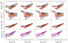 |
Fig. 1. Comparison between SPIDER (grey region), ATLAS3D (red region), MaNGA DynPop (orange region) and the theoretical Mtot–M* relation from Moster et al. (2013) (pink region) with IllustrisTNG simulations having differing astrophysical feedback parameters. Each row in the plot corresponds to a different scaling relation, from top to bottom: stellar half-mass radius, R*, 1/2, DM fraction within R*, 1/2, fDM(< R*, 1/2), DM mass within R*, 1/2, MDM, 1/2, and total (virial) mass, Mtot, as a function of stellar mass, M*. Each column shows the effect of varying one of the four astrophysical parameters. The continuous coloured lines associated to the coloured regions represent the 16th, 50th (median) and 84th percentile of the respective observational dataset distributions. The scatter of the Moster et al. (2013) theoretical relation is taken to be the mean of the scatter of the Mtot-M* relation from Posti et al. (2019). |
We can see from Fig. 1 that all simulated trends slightly overestimate the observations, except for the Mtot–M* relation, where the simulated points are largely compatible with the theoretical relation from Moster et al. (2013). At fixed stellar mass, an increase in half-mass radius, dark matter fraction, dark matter mass within the half-mass radius and total mass is observed with increasing ASN1, similarly to the LTG case studied in Paper I. Varying ASN2 results in a slight increase in the number of high-mass galaxies as ASN2 decreases. These galaxies consistently show systematically lower values of R*, 1/2, fDM(< R*, 1/2) and Mtot compared to galaxies in simulations with higher ASN2 values. This contrasts with Paper I, where a decrease in ASN2 led to higher values of R*, 1/2, fDM(< R*, 1/2) and MDM, 1/2. Nonetheless, the increase in the number of high-mass galaxies for lower ASN2 values is less pronounced than observed in Paper I.
Interestingly, the effects of varying AAGN1 and AAGN2 are negligible even with high-mass early-type galaxies, contrary to what is expected in the literature from simulations, semi-analytical models and observations (Dubois et al. 2016; De Lucia et al. 2017, 2024). This, however, may be due to the fact that only these peculiar parameters for AGN feedback have negligible impact on the scaling relations for ETGs, and other parameters may influence the massive end of the scaling relations better than AAGN1 and AAGN2. In the new CAMELS simulations (Ni et al. 2023), other AGN-feedback parameters are avaliable, so in future works it may be possible to constrain these other parameters following an analogous procedure to the one used in this work.
Fig. 2 shows, instead, the effects of changing the cosmology on the four scaling relations. We can see that the effects are identical to the effects on LTGs studied in Paper I, where variations in Ωm yield the greatest differences among simulations, while σ8 has a negligible impact across simulations. This is to be expected, given that changing the values of cosmological parameters (e.g. Ωm) should affect the internal galaxy properties in a way that is independent of galaxy type as far as the direction of the shift is concerned, while specific differences due to the different assembly history between ETGs and LTGs produces different magnitudes of variations.
3.2. Number of galaxies in the simulations
In Paper I, our primary focus was to examine the dependence of scaling relations on astrophysical and cosmological parameters and compare them with observations. We did not specifically emphasise their distribution in terms of stellar mass. In this subsection, we investigate how the number of ETGs and LTGs, in a given simulation, changes as a function of the cosmological and astrophysical parameters. In particular, the number of ETGs in the simulations is systematically lower than the number of LTGs, mainly due to their higher mass and the relatively small cosmological volume of the CAMELS simulations.
Fig. 3 shows the trends of the number of galaxies (ETGs and LTGs, respectively, on the top and bottom row) with respect to the most significant astrophysical parameters3. To assess monotonical correlations, we also conducted a hypothesis test for each parameter using Spearman’s correlation coefficient as the test statistic, with a confidence level set at 99.7 per cent. The Spearman correlation indexes, along with their corresponding p-values, are presented for both ETGs and LTGs in Table 2.
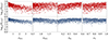 |
Fig. 3. Number of galaxies as a function of the cosmological and astrophysical parameters for each CAMELS IllustrisTNG simulation. Top row shows the number of ETGs, while bottom row shows the number of LTGs. Each column is associated to a different parameter. For each plot, for a fixed value of one of the parameters, the trends with respect to the other parameters are the same as those shown in the other panels. Parameters AAGN1 and AAGN2 are not shown for convenience. |
From Fig. 3, we observe that ETGs exhibit more scattered trends with respect to the corresponding LTG trends. For LTGs, both trends with ASN1 and ASN2 are decreasing, with ASN1 showing a notably steeper decline. This is expected, given that a higher supernovae feedback corresponds to a lower number of late-type galaxies because of quenching. On the other hand, for ETGs, we find that the trend with ASN1 is analogous to that of LTGs, while there is no trend with ASN2, indicating that an increased energy per unit SFR has much more effect on quenching ETGs at z = 0 than an increased wind velocity.
The trend of the number of both LTGs and ETGs with Ωm is increasing, indicating that in a Universe with a larger DM content, more DM halos are formed. The trend with σ8 is instead flat for LTGs, while for ETGs the trend is slightly increasing, possibly due to the fact that high-σ8 cosmologies lead to an earlier formation of high-mass clusters, and as a consequence, a higher number of mergers inside the clusters.
4. Comparison between simulations and observational datasets
In this section, we first introduce an updated methodology for ranking simulations based on their closeness with observational datasets. Subsequently, we analyse the behaviour of the fiducial and the IllustrisTNG best-fit simulation from Paper I with respect to the observational trends from SPARC, ATLAS3D and MaNGA DynPop. We proceed by identifying the best-fit simulations with respect to each of the three observational datasets, by using the procedure detailed in Section 4.1. Lastly, we determine the best-fit simulations by considering both LTGs and ETGs in the observational samples, concluding with a comparison between the observed datasets and the original IllustrisTNG simulations. For this analysis, we consider three different scaling relations: R*, 1/2–M*, fDM(< R*, 1/2)–M*, and MDM, 1/2–M*.
4.1. Ranking of simulations
Following Paper I, for each of the three observational datasets (SPIDER, ATLAS3D, MaNGA DynPop) we rank how well each simulation fits the data by considering the cumulative reduced chi-squared, which is given by the sum of the reduced chi-squared for each of the three scaling relations considered in the analysis. In Paper I, we defined the reduced chi-squared for a single scaling relation as
![Mathematical equation: $$ \begin{aligned} \tilde{\chi }^{2}_{\mathrm{rel}}=\frac{1}{N_{\mathrm{sim}}-1}\sum _{i=1}^{N_{\text{ sim}}}\frac{[{ y}_{\text{ sim,} i}-f_{\text{ rel}}(x_{\text{ sim,} i})]^{2}}{\sigma _{\text{ rel},i}^2}, \end{aligned} $$](/articles/aa/full_html/2025/01/aa51702-24/aa51702-24-eq2.gif) (1)
(1)
where (xsim, i, ysim, i) are the Nsim points from the simulation in the considered scaling relation parameter space, frel is the observed scaling relation median trend’s linear interpolation function, and σrel, i is given by the mean between σ− and σ+, which are the differences, in absolute value, between the linear interpolated functions of the 16th and the 84th percentile trends associated to the observed scaling relation, respectively, and the interpolated median trend, each evaluated at xsim, i. In this work, however, we use a slightly different definition for the reduced chi-squared:
![Mathematical equation: $$ \begin{aligned} \tilde{\chi }^{2}_{\text{ rel}}=\frac{1}{N_{\text{ sim}}-1}\,\sum _{i=1}^{N_{\text{ sim}}}\frac{[{ y}_{\text{ sim,} i}-\mathcal{N} (f_{\text{ rel}}(x_{\text{ sim,} i}),\sigma _{\text{ rel},i})]^{2}}{\sigma _{\text{ rel},i}^2}\cdot \end{aligned} $$](/articles/aa/full_html/2025/01/aa51702-24/aa51702-24-eq3.gif) (2)
(2)
The main difference between the new definition and the one used in Paper I is at the numerator, where this time we evaluate the difference between the y component of the simulated point, ysim, i, and a randomly extracted point from a Gaussian distribution, 𝒩, centred on the median of the observed scaling relation, with standard deviation equal to σrel, i. This is done in order to obtain more realistic uncertainties.
In comparison to the previous paper, we also ensure that the simulations have realistic distributions in terms of the galaxy stellar mass. Specifically, we avoid situations where all the galaxies are clustered in a very tight range of stellar mass or where the distribution in terms of stellar mass is strongly discontinuous. To achieve this, we bin the quantities associated to the scaling relations, for example the stellar half-mass radius, with respect to values of stellar mass. We then filter out simulations that have less than one galaxy in each bin of stellar mass, using the same bin edges as those employed for the analogous binning of the observational trends. To lessen the constraint imposed by this filtering procedure, we exclude the very first and last bins with respect to stellar mass in this procedure.
We evaluated the values of  for all remaining CAMELS simulations from the filtering procedure, and rank the simulations according to its value. We then considered the lowest
  -value simulation as the best-fit simulation for a given observational dataset.
The uncertainty on the cosmological and astrophysical parameters is determined by performing 100 bootstrap resamplings of both the observational datasets and simulated data points, with each resampling being a copy of the original dataset having some of the galaxies substituted by copies of other galaxies in the same dataset. This is accomplished by using the MATHEMATICA resource function BOOTSTRAPSTATISTICS (more informations are available in Paper I). Given a certain observational dataset, for each resampling, the simulations are ranked based on the value of  . By picking the best-fit simulation for each resampling, we obtain a sample of 100 best-fit simulations. We evaluate the empirical cumulative distribution functions (CDFs) for each cosmological and astrophysical parameter of this sample, via the formula
 (3)
(3)
with n = 100 being the dimension of the sample. We then smooth the empirical CDFs with a Gaussian kernel having standard deviation σ = 1, in order to avoid issues deriving by the discrete nature of the empirical CDF. We then obtain the parameter estimates from the smoothed CDFs, by considering the associated 16th, 50th (median) and 84th percentiles. The results are listed in Table 3. The constraints considering the 16th, 50th and 84th percentile taken directly from the empirical CDFs instead are detailed in Appendix B1.
Constraints on cosmological and astrophysical parameters, obtained by bootstrapping both observational and simulated datasets, and taking for each resampling the best-fit simulation.
4.2. CAMELS fiducial simulation comparison with observations
As a preliminary check, we verify if the fiducial IllustrisTNG simulation from CAMELS reproduces accurately the observational trends from SPIDER, ATLAS3D, and MaNGA DynPop for the ETG sample. The procedure to obtain the observational trends is the same as in Paper I.
Fig. 4 shows the comparison between the simulated ETGs from the fiducial IllustrisTNG CAMELS simulation, 1P_1_0, and the observational trends. Quantitatively, the cumulative reduced chi-squared,  , is
, is  with respect to SPIDER,
  with respect to ATLAS3D and
  with respect to MaNGA DynPop. The associated ranks are equal to 316, 354 and 353, respectively, where a rank of 1 is associated to the best-fit simulation. This means that the fiducial simulation is far from being the better fit for all of the three observational trends.
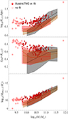 |
Fig. 4. Comparison of fiducial IllustrisTNG simulation with observational trends. From top to bottom: stellar half-mass radius, R*, 1/2, DM fraction within R*, 1/2, fDM, and DM mass within R*, 1/2, MDM, 1/2, as a function of stellar mass, M*, for the fiducial IllustrisTNG simulation 1P_1_0, compared with the corresponding SPIDER (black curves), ATLAS3D (dark red curves) and MaNGA DynPop (orange curves) trends. The shaded areas represent the scatter of the observed relations, given by the difference between the 16th and the 84th percentiles with the median. As an example, the open circles are galaxies not used for the evaluation of the cumulative reduced chi-squared associated to the ATLAS3D observational trend in Section 4.2. |
Visually, one can see that there is a systematic overestimate of the considered quantities, at fixed stellar mass, with respect to the observational values. This finding aligns with the overestimation observed in Paper I for the fiducial IllustrisTNG simulation, concerning LTGs. However, for ETGs, the discrepancy is even more pronounced, with the simulated trends being compatible within 1σ only with the SPIDER observations, and only at high mass (log10(M*/M⊙)≳10.5).
4.3. Consistency of ETG results with IllustrisTNG LTG best-fit simulation
In Paper I, we found that the CAMELS simulation LH_698, with parameters Ωm = 0.27, σ8 = 0.83, S8 = 0.78, ASN1 = 0.48, ASN2 = 1.24, AAGN1 = 2.53, and AAGN2 = 1.79, is the best-fit simulation reproducing the observed trends for LTGs from SPARC (Lelli et al. 2016). In Fig. 5 we show the comparison between the simulated ETGs from this simulation and the observational trends from SPIDER, ATLAS3D, and MaNGA DynPop.
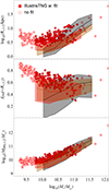 |
Fig. 5. Same as Fig. 4, but for the best-fit simulation LH_698, found in Paper I to be the best-fit simulation between the simulated LTG data and the SPARC trends. |
From Fig. 5, we can see that the simulation LH_698 is not reproducing the observed correlations for the ETG sample: for this simulation the cumulative reduced chi-squared is  with respect to SPIDER,
  with respect to ATLAS3D and
  with respect to MaNGA DynPop, with an ordered rank of 324, 150 and 157, respectively.
While in the case of SPIDER the ranking is slightly higher than the ranking of the fiducial simulation, in the case of ATLAS3D and MaNGA DynPop the ranking is much lower, showing a slightly better compatibility of this simulation with the observational datasets. The comparison between the values of the two simulations is reported in Table 4.
Comparison between the cumulative reduced chi-squared for the fiducial IllustrisTNG 1P_1_0 simulation and the IllustrisTNG best-fit simulation LH_698 from Paper I.
Visually, we can see from the figure that the simulated ETG sample systematically overestimates all three observational trends, except at high mass (log10(M*/M⊙)≳10.7). Even at high mass, however, the improved alignment between simulated ETGs from the best-fit simulation of Paper I and observational trends is primarily attributed to the greater dispersion exhibited by the simulated data points.
4.4. Best fit to the observations
In Sections 4.2 and 4.3, we have seen that neither the fiducial nor the best-fit simulation of Paper I accurately reproduce the observed trends from SPARC, ATLAS3D and MaNGA DynPop. We thus proceed with the method detailed in Section 4.1, to find the best-fit simulation for the various observational trends.
4.4.1. SPIDER
For the SPIDER trends, we find that the best-fit simulation is the simulation LH_523, having the following cosmological and astrophysical parameters: Ωm = 0.24, σ8 = 0.84, S8 = 0.74, ASN1 = 1.38, ASN2 = 0.68, AAGN1 = 1.24, and AAGN2 = 1.19, where the value of S8 has been determined from the definition,  . The cumulative reduced chi-squared associated to this simulation is
  .
.
The first column of Fig. 6 illustrates the comparison between the ETGs of this simulation and the observed SPIDER trends. The figures reveals a slight overestimation by the simulated galaxies of the size-mass relation. The simulation also shows a lack of galaxies in the low-mass tail of the observational trends. This is especially evident in the size-mass relation.
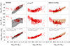 |
Fig. 6. Each column of this figure is the same as in Fig. 4, but for the best-fit simulation associated to SPIDER (left column), ATLAS3D (center column) and MaNGA DynPop (right column) observational trends. Red squares are the simulated galaxies. Filled red squares are for galaxies used for the evaluation of the cumulative reduced chi-squared with respect to the associated observational trend. |
Through bootstrap resampling, we derived the constraints for the cosmological and astrophysical parameters reported in the first row of Table 3. Results show a slightly lower value of Ωm, compatible with Dark Energy Survey and Kilo-Degree Survey Collaboration (2023) and Paper I results, but not with Planck Collaboration VI (2020) within 1σ. The values of σ8 and S8 are instead compatible with both results, along with Paper I. Regarding the astrophysical parameter ASN1, SPIDER constraints suggest a higher estimate compared to the fiducial unit value from CAMELS, incompatible with the results of Paper I that showed a value of ASN1 equal to  by comparing simulations with the SPARC LTG sample, which is instead lower than the fiducial unit value. Correspondingly, we see a lower value of ASN2 than the fiducial value, also incompatible with Paper I results that show a value of ASN2 equal to
  . Constraints on AAGN1 and AAGN2 are not particularly significant, with AAGN1 unconstrained and AAGN2 compatible within the uncertainties with the fiducial value.
4.4.2. ATLAS3D
For the trends in the ATLAS3D sample, we find that the best-fit simulation is the simulation LH_797, having the following cosmological and astrophysical parameters: Ωm = 0.22, σ8 = 0.89, S8 = 0.77, ASN1 = 0.28, ASN2 = 1.96, AAGN1 = 0.45, and AAGN2 = 1.15, with a cumulative reduced chi-squared value of  .
.
The central column of Fig. 6 shows the comparison between the ETGs of this simulation and the observed ATLAS3D trends. From the figure, we can see that the simulated galaxies closely match the observed ATLAS3D trends, albeit with a slight overestimate of the three quantities at fixed stellar mass, which is accentuated for the size-mass relation at the high-mass end.
Cosmological constraints from ATLAS3D, reported in the second row of Table 3, are compatible with constraints from SPIDER and Paper I within the uncertainties considered. The parameter Ωm, constrained from ATLAS3D, is not compatible with both Planck Collaboration VI (2020) and Dark Energy Survey and Kilo-Degree Survey Collaboration (2023) results within 1σ, but is closer to the latter. The constraint of σ8 instead is compatible with both results, while the constraint of S8 is only compatible with Dark Energy Survey and Kilo-Degree Survey Collaboration (2023) results. The values of ASN1 and ASN2 obtained show an inversion compared to the ones from SPIDER: ASN1 is significantly lower, while ASN2 is higher than the respective fiducial values, although the latter remains compatible with the fiducial value within the uncertainties. Both supernovae feedback parameters are compatible with the results found in Paper I.
4.4.3. MaNGA DynPop
For the MaNGA DynPop trends, we find that the best-fit simulation is the simulation LH_586, having the following cosmological and astrophysical parameters: Ωm = 0.16, σ8 = 0.97, S8 = 0.70, ASN1 = 0.30, ASN2 = 1.61, AAGN1 = 2.71, and AAGN2 = 1.77, with a cumulative reduced chi-squared value of  .
.
The right column of Fig. 6 shows the comparison between the ETGs of this simulation and the observed MaNGA DynPop trends. From the figure, we can see that there is a low agreement between the best-fit simulation and the observed trends. In particular, there is a systematic overestimation of the size in the size-mass relation, and a systematic underestimate of dark matter mass in the MDM, 1/2–M* relation, which in turn leads to a systematic underestimate of DM fraction in the fDM(< R*, 1/2)–M* relation.
The constraints for MaNGA DynPop are reported in the third row of Table 3. In this case, the value of Ωm is much lower than the ones obtained from the fitting procedure with SPIDER and ATLAS3D observations, other than the results from Paper I, while the value of σ8 is instead compatible with all of them within the uncertainties, albeit with a very high median value. This produces a very low value of S8, not compatible with Planck Collaboration VI (2020) nor Dark Energy Survey and Kilo-Degree Survey Collaboration (2023) results. The value of S8 is however compatible with the values inferred from SPIDER and ATLAS3D observations, and from SPARC in Paper I, within the uncertainties. Supernovae feedback parameters are in agreement with the constraints found for ATLAS3D. AGN feedback parameters are unconstrained.
4.5. A best-fit solution for ETGs and LTGs
In Section 4.2, we identified a systematic upwards shift of all three scaling relations in the fiducial CAMELS simulation, with respect to the observational trends. In Section 4.3, we also identified that the simulation identified as the best-fit for SPARC in Paper I ranks low when comparing the corresponding ETG galaxies with observations. The main cause of this could be the fact that we did not constrain both LTGs and ETGs simultaneously: consequently, the procedure primarily aimed at finding the LTG population that best matched the observations, without ensuring that the simulation also accurately represented the behaviour of ETGs.
We have thus repeated the chi-squared procedure by constraining both LTGs against SPARC and the ETGs against the three observational ETG trends (SPIDER, ATLAS3D, and MaNGA DynPop), then obtaining the cumulative reduced chi-squared for both ETGs and LTGs simultaneously,  , by evaluating the sum of the cumulative reduced chi-squared for each of the two galaxy types and ranking the simulations with respect to this sum. We find that, for SPIDER, the best-fit simulation is the LH_325 simulation, while for both ATLAS3D and MaNGA DynPop the best-fit simulation is the LH_797 simulation. The former has the following cosmological and astrophysical parameters: Ωm = 0.24, σ8 = 0.61, S8 = 0.55, ASN1 = 0.74, ASN2 = 0.83, AAGN1 = 0.38, and AAGN2 = 1.02, with a cumulative reduced chi-squared associated to SPIDER of
  . The latter, which is also the best-fit simulation with respect to ATLAS3D alone, has instead the following parameters: Ωm = 0.22, σ8 = 0.89, S8 = 0.77, ASN1 = 0.28, ASN2 = 1.96, AAGN1 = 0.45, and AAGN2 = 1.15. The cumulative reduced chi-squared associated to ATLAS3D is
  , while the one associated to MaNGA DynPop is higher,
  , implying a lower agreement between MaNGA DynPop and this best-fit simulation.
By repeating the bootstrap procedure detailed in Section 4.1, including also SPARC, we obtained the constraints reported in the first three rows of Table 5. The constraints considering the 16th, 50th and 84th percentile taken directly from the empirical CDFs instead are reported in Appendix B2. The heat maps showing the regions of lowest  are, instead, described and shown in Appendix C. An assessment of the effects of a potential selection bias due to the fact that there is a higher number of low-mass galaxies with respect to high-mass galaxies is, finally, discussed in Appendix D.
Constraints on cosmological and astrophysical parameters, obtained by bootstrapping the observational (including SPARC and MaNGA DynPop LTGs) and simulated datasets, and taking for each resampling the best-fit simulation.
Regarding the cosmological parameters, adding the comparison between simulated LTGs and SPARC to the analysis does not change significantly the parameters for SPIDER, while for ATLAS3D there is a slight increase in the median value of σ8 and S8. The most significant impact is observed on the MaNGA DynPop constraints, where adjustments in Ωm and σ8 have resulted in S8 being aligned with the findings of the Dark Energy Survey and Kilo-Degree Survey Collaboration (2023), albeit incompatible with those of the Planck Collaboration VI (2020). Overall, in all three scenarios there is now a tendency towards lower values of S8. This is compatible with the fact that, in the S8 tension framework, probes of the local universe show predictions of S8 which are systematically lower than early-epoch investigations (see Abdalla et al. 2022, Section 5).
Regarding the astrophysical parameters, we find that adding the comparison between simulated LTGs and SPARC to the analysis results in a reduction of SPIDER’s constraint on ASN1 below the fiducial unit value, with all three values compatible within the uncertainties. On the other hand, the effects on ASN2, AAGN1, and AAGN2 are negligible.
Fig. 7 shows the comparison between both LTGs and ETGs from these simulations and the observed trends. While there is a general agreement between observed and simulated galaxies, the left column reveals a high scatter associated to the simulated LTGs in the size-mass relation. We also notice a systematic overestimate of stellar half-mass radii at high stellar mass. Overall, the agreement is poorer with MaNGA DynPop than with ATLAS3D.
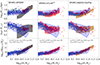 |
Fig. 7. Same as Fig. 6, but considering both simulated LTGs (blue points) and simulated ETGs (red points). The blue region is the SPARC observational trend from Paper I. |
Summing up, we do not find the best-fit simulation of Paper I even when constraining both LTGs and ETGs. Instead, we find that a value of S8 generally compatible with local Universe results such as Dark Energy Survey and Kilo-Degree Survey Collaboration (2023), and for ATLAS3D and MaNGA DynPop a common best-fit simulation, with more reasonable cosmological parameters for the latter. In all cases, we have a low value for ASN1, recovering the main result from Paper I for all three observational datasets.
In a second analysis, we tried to constrain both LTGs and ETGs associated to the MaNGA DynPop sample. This is important because, differently from the analysis described so far, in this case the two sub-samples come from the same sample, and thus rely on the same data analysis and modelling assumptions. Using the same procedure we used in this section, we found that the best-fit simulation is the simulation LH_531, with the following cosmological parameters: Ωm = 0.24, σ8 = 0.93, S8 = 0.84, ASN1 = 2.43, ASN2 = 0.59, AAGN1 = 0.44, and AAGN2 = 0.95, with a cumulative reduced chi-squared of  , indicating a rather poor fit. From Fig. 8, a clear distinction emerges: the observed ETG sample trends have a markedly different slope and normalisation with respect to the corresponding LTG trends, a dichotomy which is not observed in any simulated galaxy sample. The best-fit simulation, aimed at simultaneously reproducing both trends, notably lacks simulated ETGs within the orange region for stellar masses lower than 1010.6 M⊙. This could imply a failure in the CAMELS IllustrisTNG simulations in reproducing dichotomic trends for scaling relations that span a wider range of galaxy types.
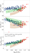 |
Fig. 8. Same as Fig. 4, but for the best-fit simulation to the whole MaNGA DynPop sample, LH_531. The blue squares indicate simulated LTG galaxies, while red squares indicate simulated ETG galaxies. The open squares are galaxies not used for the evaluation of the cumulative reduced chi-squared associated to the respective observational trend. The dark orange region is associated to the observed MaNGA DynPop ETG sample, while the green region is associated to the LTG sample. |
By repeating the bootstrap procedure detailed in Section 4.1, comparing both the LTG and ETG observed trends from MaNGA DynPop with the respective types of simulated galaxies, we obtained the constraints reported in the fourth row of Table 5. Constraints for S8 are compatible with both Planck Collaboration VI (2020) and Dark Energy Survey and Kilo-Degree Survey Collaboration (2023) results within 1σ. Constraints for ASN1 show a very high uncertainty, possibly as a consequence of the aforementioned dichotomy. The constraint for ASN1 is also higher than the fiducial value, but this seems to be mainly an effect of neglecting the contribution of the gas mass for the observed galaxies: taking it into account in the analysis as described in Appendix A, we obtain a result consistent with the constraints using SPARC as the observational LTG sample.
4.6. Comparison with original IllustrisTNG simulations
Another possibility for the shifts found among data and simulations, which we did not account for in Paper I, is the fact that there could be mass and/or volume resolution effects at play that skew the data points upwards with respect to a converged simulation.
To investigate any potential systematic shifts between observations and the fiducial CAMELS simulation that may arise from convergence issues due to a low mass and volume resolution of CAMELS, we have also analysed the same scaling relations used in Section 4, but using the subhalos from TNG-300, TNG-100 and TNG-50. Fig. 9 shows a comparison between the trends of the fiducial CAMELS simulation and those of the three TNG simulations: in all four cases, the galaxies have been binned in bins of stellar mass, with uncertainties along the y-axis evaluated as the standard deviation of the corresponding values in each bin, in order to capture the general trend of the simulations, and to compare them to the observed trends.
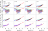 |
Fig. 9. Comparison of different IllustrisTNG suites with observational trends. From top to bottom: stellar half-mass radius, DM fraction within the stellar half-mass radius and DM mass within the stellar half-mass radius as a function of stellar mass, for fiducial CAMELS simulation (first column), TNG-300 (second column), TNG-100 (third column) and TNG-50 (fourth column). The simulated galaxies for all four simulations have been binned in bins of stellar mass (red points for ETGs, blue points for LTGs, uncertainty given by the standard deviation of the y-values in the bins). The coloured regions have the same meaning as in Figs. 1 and 7. |
As one can see from the figure, for ETGs CAMELS and TNG-300 overestimate the observed trends, especially on the low-mass end of the observed trends; TNG-100, on the other hand, is much closer to the median observed trends. TNG-50, instead, seems to slightly underestimate the observed trends, especially SPIDER. Moreover, for LTGs, we can see an overestimate of CAMELS and TNG-300 with respect to the SPARC observational trends, with TNG-100 and TNG-50 better reproducing them, but we can also observe that CAMELS and TNG-300 reproduce the R*, 1/2-M* and MDM, 1/2-M* trends of MaNGA DynPop for the LTG sample better than or equally good than TNG-100 and TNG-50. In particular, both TNG-100 and TNG-50 underestimate the MaNGA DynPop (LTGs) MDM, 1/2-M* trend, while TNG-300 and CAMELS reproduce it correctly. Moreover, in both CAMELS and the three original TNG simulations, we can see that the dichotomic trend of the MaNGA DynPop sample is not reproduced; rather, both LTGs and ETGs tend to follow roughly the same trend.
Finally, to ensure that these effects are indeed due to the mass resolution rather than to other factors (e.g. the different volumes in the three TNG simulations) we compared the three simulations TNG100-1, TNG100-2, and TNG100-3, which have the same fixed volume but different mass resolutions. In particular, TNG100-2 has roughly the same mass resolution as TNG300-1, as can be seen from Table 1. Results show that the effects of changing resolution at fixed volume are the same of those shown in Fig. 9, that is, lower resolutions correspond to a systematic increase in DM fraction within the stellar half-mass radius.
These results seem to imply that:
-
Even accounting for convergence effects related to the mass and/or the spatial resolution of the CAMELS fiducial simulation, the higher-resolution simulations still fail to fully replicate all observed trends. On the contrary, in some instances lower-resolution simulations perform better in matching observed trends than their higher-resolution counterparts, as in the case of the LTG sample of MaNGA DynPop;
-
IllustrisTNG, similarly to CAMELS simulations, fails to reproduce observed dichotomic trends between LTGs and ETGs. The subhalos are aligned at all resolutions, and roughly follow the same trend, differently from the observed scaling relation trends. The fact that CAMELS and TNG-300 do not manage to reproduce the MaNGA DynPop observed trend for ETGs could be a consequence of this point.
4.7. Comparison with literature
In the past, studying the impact of the variation of cosmological and astrophysical parameters on the physics of galaxies was very hard, given the computational cost of running multiple hydrodynamical simulations. There have been, however, some initial attempts to produce simulations with differing values of astrophysical parameters and study the effect that their variation have on galaxies. One of such attempts was the SEAGLE programme (Mukherjee et al. 2018, 2021, 2022), which used simulated strong gravitational lenses from the EAGLE simulations to study galaxy formation. In particular, Mukherjee et al. (2021) explore the impact of SN- and AGN-feedback parameters on early-type deflectors’ observables. They find that a low stellar feedback better matches the size-mass relation derived from the Sloan Lens ACS Survey (SLACS) observations, which is consistent with our findings. However, they also find that different AGN feedback parameters, such as the viscosity parameter or the AGN heating temperature, have an important effect on the simulations. Given that the kinetic AGN feedback parameters AAGN1 and AAGN2 seem to have a negligible impact on simulations, in future works we will analyse the new CAMELS simulations, that vary more AGN feedback parameters, which could be more impactful on the scaling relation trends (Tortora et al., in prep.).
With better computational power and simulation techniques, simulation suites such as CAMELS became available. There have been many works in the literature that used these simulations to infer the values of cosmological parameters, for example by using photometry of galaxies (Hahn et al. 2024), the physical properties of single galaxies (Villaescusa-Navarro et al. 2022) or of multiple galaxies (Chawak et al. 2024). Using the photometry of multiple galaxies, Hahn et al. (2024) manage to constrain with remarkable accuracy the values of Ωm and σ8, while the work of Chawak et al. (2024) shows that, by training a neural network to obtain the cosmological and astrophysical parameters of CAMELS simulations given the properties of two galaxies, the recovery of σ8 and ASN2 is weak (with the recovery getting better by using ten galaxies instead of two), while AGN-feedback parameters are completely unconstrained. These results are also consistent with our findings.
Other attempts in literature to constrain cosmological and astrophysical parameters with the use of simulations include HIFLOW (Hassan et al. 2022), a generative model for the estimation of the probability density function of the target observable (e.g. cosmological parameters), based on the masked autoregressive flow method (Papamakarios et al. 2017). The advantage with respect to our method is that HIFLOW manages to find the correct posterior distribution of the cosmological parameters Ωm and σ8 given the observed HI maps from CAMELS and uniform priors. A disadvantage is that the method is weakly dependant on the value of the astrophysical parameters.
Another approach is to train a neural network to work as an emulator of the CAMELS simulations, to perform fast implicit likelihood inference (ILI, Jo et al. 2023) of the cosmological and astrophysical parameters by substituting the simulations with the emulators. By using the cosmic star formation rate density (SFRD) and the stellar mass functions (SMF), the method is able to obtain the posterior distributions for Ωm, σ8 and the SN- and AGN-feedback parameters. By applying this procedure on actual observational data from Leja et al. (2020, 2022); Jo et al. (2023) find very extreme values for the cosmological parameters Ωm and σ8, which they report is due to CAMELS resolution effects and degeneracies with the astrophysical parameters. This issue, however, seems to not be present in our constraining procedure. They also notice how AGN-feedback parameters AAGN1 and AAGN2 are weakly constrained with their procedure, due to a low influence of kinetic AGN feedback on formation of high stellar mass galaxies and star formation in massive galaxies. This is in agreement with our results. There exist many other projects that try to make simulation-based inference of cosmological and astrophysical parameters, for example by using graph neural networks to obtain information from galaxy distributions (Roncoli et al. 2023), but an extensive review of these is outside the scope of our work.
5. Conclusions
In this work we expanded the CASCO project (Busillo et al. 2023) by extending the analysis to early-type galaxies. We considered three different observational datasets (SPIDER, ATLAS3D, and MaNGA DynPop) and updated both the definition and the evaluation procedure of the reduced chi-squared, by considering a selection of only those simulations that have a uniform coverage in stellar mass. Our main results are the following:
-
We have shown that both the fiducial simulation, which is the one that has the cosmological and astrophysical parameters equal to the original IllustrisTNG simulation, and the best-fit simulation of Paper I that we found for LTGs are not a good fit for the simulated early-type galaxies. Both simulations systematically overestimate all three observational trends. Even when constraining both LTGs and ETGs at the same time, we do not recover the two simulations as the best-fit ones.
-
We ran our procedure (see Section 4.1), searching for the best-fit between the simulated ETGs and the three different observational trends. We found for the SPIDER sample that the best-fit simulation is the simulation LH_523, with constraints that show values for ASN1 and ASN2 higher and lower than the fiducial unit values from CAMELS, respectively. This is incompatible with the results obtained in Paper I from the SPARC observational sample, which showed ASN1 lower and ASN2 higher than the respective fiducial values. For the ATLAS3D and MaNGA DynPop samples, we instead found values of the astrophysical parameters in line with the results from Paper I, although the latter shows respectively lower and higher values of Ωm and σ8 than those from Planck Collaboration VI (2020) and Dark Energy Survey and Kilo-Degree Survey Collaboration (2023), resulting in a very low value of S8. Constraints from the ranking procedure are thus strongly affected by the properties of the reference observational trends. Similarly to Paper I, we find also in this case that with all observational samples the AGN-feedback parameters AAGN1 and AAGN2 are unconstrained.
-
Constraints are modified when considering also LTG observations along with ETG observations. Using SPARC as the observational LTG sample and performing the bootstrap procedure, we obtain a lower value of S8 with respect to Planck Collaboration VI (2020) and a lower value of ASN1 with respect to the fiducial CAMELS unit value for all three ETG observational datasets, recovering the main result of Paper I. Using the full MaNGA DynPop sample (including both ETGs and LTGs) results in an S8 value compatible with Dark Energy Survey and Kilo-Degree Survey Collaboration (2023) and a very large uncertainty on ASN1, possibly due to a dichotomic trend between the ETGs and the LTGs in the MaNGA DynPop sample.
-
To check for a possible systematic effect due to the limited numerical resolution in CAMELS, we compared the fiducial simulation with the original Illustris simulations. We have considered ETGs and LTGs from TNG-300, TNG-100, and TNG-50, and showed that both the fiducial CAMELS simulation and TNG-300 are compatible with each other as far as the behaviour with respect to the observational trends is concerned, with both simulations overestimating the observed trends in a similar way, both for LTGs and ETGs. Results suggest that systematic effects associated to both simulations and observational datasets are influencing the alignment of the respective trends. In particular a lack of convergence caused by a low particle mass resolution does not imply that simulations with low resolution behave necessarily worse than higher resolution ones.
In this work, we have seen that there are many caveats to be considered before fully exploiting the predictive power of galaxy scaling relations to constrain cosmology and astrophysics. Expanding our scope to early-type galaxies has shown that fitting only one type of galaxy to the observational datasets does not imply that the fit generalises to other types of galaxies, and we have shown that, even by changing the reference observational trends, the constraints show a significant variation.
We have also shown that, despite the low mass and volume resolution of CAMELS, the fiducial simulation is able to reproduce the MaNGA DynPop observational trend for LTGs. The comparison with the original TNG simulations shows that, in regards to reproducing observed scaling relations, the IllustrisTNG suite of CAMELS is still a reliable tool, even with the presence of possible convergence effects. Both CAMELS and the original IllustrisTNG simulations, however, fail in reproducing the dichotomic trend shown by the full MaNGA DynPop observational sample. This could imply that there are some limitations in how subhalos properties are obtained in the simulations (and as such, showing some of the limits of the sub-grid approach used to replicate the baryonic processes in the IllustrisTNG subhalos), or in the various observational samples used for the comparisons, given that different approaches are used to obtain them.
For the future, we plan to analyse the evolution of simulated scaling relations across cosmic time (Tortora et al. 2014c, 2018; Sharma et al. 2022), to check whether the simulations manage to reproduce correctly the observations also at high redshift. Constraints of scaling relations at high redshift could also provide some information about past values of Ωm and a possible evolution of σ8 with cosmic time (Adil et al. 2024). Moreover, in this work we fixed for simplicity the sub-grid physics to the one from IllustrisTNG. Given that no recipe is a perfect representation of the real astrophysical processes that occur in the Universe, it is important to check that the constraining procedure is robust with respect to the change of subgrid recipe. While some of this analysis has been performed for LTGs only in Paper I, in future works we will explore more in detail the impact of changing the sub-grid physics, especially with the new CAMELS simulations, which provide new suites such as Magneticum and EAGLE.
Other simulations from CAMELS, with higher resolution and larger volumes, could also allow us to check further for convergence effects. In future works, especially by leveraging on the enhanced statistics at high mass by using the simulations having larger volumes, it may be possible to check the effects that additional AGN-feedback parameters present in the new CAMELS simulations (Ni et al. 2023), such as the normalisation factor for the Bondi rate for the accretion onto SMBHs or the threshold between the low-accretion and high-accretion states of AGN feedback (Weinberger et al. 2017), have on the scaling relations, and in particular on the transition mass scale for scaling relations such as the total-stellar mass relation, the so-called golden mass (Tortora et al., in prep.).
Future surveys, like the Euclid Wide Survey and the Cosmic Dawn Survey (Euclid Collaboration 2022a,b), will both detect much larger samples of rare, massive galaxies and observe galaxies up to very high redshifts. In particular, it is expected that around 105 strong gravitational lenses will be found by Euclid (Collett 2015), enabling the determination of very precise mass estimates and constraints on dark matter fraction for a substantial set of high-mass galaxies. This dataset can then be utilised for comparison with simulations. As such it is auspicable that CAMELS will allow in the future to have more statistics available, especially on the high-mass end of simulated galaxies.
For simplicity, we ignore the complexity of galaxy classification based on morphology, colour, or star formation activity, each of which can lead to different galaxy selections. Therefore, throughout this paper, we use early-type galaxies as a synonym for passive galaxies, and late-type galaxies as a synonym for star-forming galaxies.
The Jeans dynamical modelling of SPIDER galaxies is based on velocity dispersions measured within SDSS fibers, which have a fixed radius which is obviously different from the effective radii of each individual galaxies, requiring some extrapolation to the effective radius in the mass calculation, while in the ATLAS3D no extrapolation is necessary.
We avoided considering the AGN feedback parameters for convenience, but we have checked that the trends of NLTG and NETG with respect to AAGN1 and AAGN2 are constant.
Acknowledgments
V.B., C.T. and M.S. acknowledge the INAF grant 2022 LEMON.
References
- Abdalla, E., Abellán, G. F., Aboubrahim, A., et al. 2022, J. High Energy Astrophys., 34, 49 [NASA ADS] [CrossRef] [Google Scholar]
- Adil, S. A., Akarsu, Ö., Malekjani, M., et al. 2024, MNRAS, 528, L20 [Google Scholar]
- Baes, M., Mosenkov, A., Kelly, R., et al. 2024, A&A, 683, A182 [NASA ADS] [CrossRef] [EDP Sciences] [Google Scholar]
- Bernardi, M., Sheth, R. K., Domínguez Sánchez, H., et al. 2023, MNRAS, 518, 3494 [Google Scholar]
- Bisigello, L., Kuchner, U., Conselice, C. J., et al. 2020, MNRAS, 494, 2337 [NASA ADS] [CrossRef] [Google Scholar]
- Bolton, A. S., Burles, S., Koopmans, L. V. E., Treu, T., & Moustakas, L. A. 2006, ApJ, 638, 703 [NASA ADS] [CrossRef] [Google Scholar]
- Bruzual, G., & Charlot, S. 2003, MNRAS, 344, 1000 [NASA ADS] [CrossRef] [Google Scholar]
- Bundy, K., Bershady, M. A., Law, D. R., et al. 2015, ApJ, 798, 7 [Google Scholar]
- Busillo, V., Tortora, C., Napolitano, N. R., et al. 2023, MNRAS, 525, 6191 (Paper I) [NASA ADS] [CrossRef] [Google Scholar]
- Cappellari, M. 2008, MNRAS, 390, 71 [NASA ADS] [CrossRef] [Google Scholar]
- Cappellari, M. 2017, MNRAS, 466, 798 [Google Scholar]
- Cappellari, M. 2020, MNRAS, 494, 4819 [NASA ADS] [CrossRef] [Google Scholar]
- Cappellari, M. 2023, MNRAS, 526, 3273 [NASA ADS] [CrossRef] [Google Scholar]
- Cappellari, M., & Emsellem, E. 2004, PASP, 116, 138 [Google Scholar]
- Cappellari, M., Emsellem, E., Krajnović, D., et al. 2011, MNRAS, 413, 813 [Google Scholar]
- Cappellari, M., Scott, N., Alatalo, K., et al. 2013a, MNRAS, 432, 1709 [Google Scholar]
- Cappellari, M., McDermid, R. M., Alatalo, K., et al. 2013b, MNRAS, 432, 1862 [NASA ADS] [CrossRef] [Google Scholar]
- Cardelli, J. A., Clayton, G. C., & Mathis, J. S. 1989, ApJ, 345, 245 [Google Scholar]
- Chabrier, G. 2001, ApJ, 554, 1274 [NASA ADS] [CrossRef] [Google Scholar]
- Chabrier, G. 2003, PASP, 115, 763 [Google Scholar]
- Chawak, C., Villaescusa-Navarro, F., Echeverri-Rojas, N., et al. 2024, ApJ, 969, 105 [NASA ADS] [CrossRef] [Google Scholar]
- Collett, T. E. 2015, ApJ, 811, 20 [NASA ADS] [CrossRef] [Google Scholar]
- Conselice, C. J., Bluck, A. F. L., Mortlock, A., Palamara, D., & Benson, A. J. 2014, MNRAS, 444, 1125 [Google Scholar]
- Crain, R. A., Schaye, J., Bower, R. G., et al. 2015, MNRAS, 450, 1937 [NASA ADS] [CrossRef] [Google Scholar]
- Dark Energy Survey and Kilo-Degree Survey Collaboration (Abbott, T. M. C., et al.) 2023, Open J. Astrophys., 6, 36 [NASA ADS] [Google Scholar]
- De Lucia, G., Fontanot, F., & Hirschmann, M. 2017, MNRAS, 466, L88 [NASA ADS] [CrossRef] [Google Scholar]
- De Lucia, G., Fontanot, F., Xie, L., & Hirschmann, M. 2024, A&A, 687, A68 [NASA ADS] [CrossRef] [EDP Sciences] [Google Scholar]
- de Santi, N. S. M., Shao, H., Villaescusa-Navarro, F., et al. 2023, ApJ, 952, 69 [NASA ADS] [CrossRef] [Google Scholar]
- Dekel, A., & Birnboim, Y. 2004, AIP Conf. Ser., 743, 162 [NASA ADS] [CrossRef] [Google Scholar]
- Dickey, C. M., Starkenburg, T. K., Geha, M., et al. 2021, ApJ, 915, 53 [NASA ADS] [CrossRef] [Google Scholar]
- Domínguez Sánchez, H., Margalef, B., Bernardi, M., & Huertas-Company, M. 2022, MNRAS, 509, 4024 [Google Scholar]
- Dubois, Y., Peirani, S., Pichon, C., et al. 2016, MNRAS, 463, 3948 [Google Scholar]
- Echeverri-Rojas, N., Villaescusa-Navarro, F., Chawak, C., et al. 2023, ApJ, 954, 125 [NASA ADS] [CrossRef] [Google Scholar]
- Euclid Collaboration (Scaramella, R., et al.) 2022a, A&A, 662, A112 [NASA ADS] [CrossRef] [EDP Sciences] [Google Scholar]
- Euclid Collaboration (Moneti, A., et al.) 2022b, A&A, 658, A126 [NASA ADS] [CrossRef] [EDP Sciences] [Google Scholar]
- Hahn, C., Villaescusa-Navarro, F., Melchior, P., & Teyssier, R. 2024, ApJ, 966, L18 [NASA ADS] [CrossRef] [Google Scholar]
- Hassan, S., Villaescusa-Navarro, F., Wandelt, B., et al. 2022, ApJ, 937, 83 [NASA ADS] [CrossRef] [Google Scholar]
- Hunt, L. K., Tortora, C., Ginolfi, M., & Schneider, R. 2020, A&A, 643, A180 [NASA ADS] [CrossRef] [EDP Sciences] [Google Scholar]
- Ilbert, O., Arnouts, S., McCracken, H. J., et al. 2006, A&A, 457, 841 [NASA ADS] [CrossRef] [EDP Sciences] [Google Scholar]
- Jo, Y., Genel, S., Wandelt, B., et al. 2023, ApJ, 944, 67 [NASA ADS] [CrossRef] [Google Scholar]
- La Barbera, F., de Carvalho, R. R., de La Rosa, I. G., et al. 2010, MNRAS, 408, 1313 [CrossRef] [Google Scholar]
- Lee, M. E., Genel, S., Wandelt, B. D., et al. 2024, ApJ, 968, 11 [NASA ADS] [CrossRef] [Google Scholar]
- Leja, J., Speagle, J. S., Johnson, B. D., et al. 2020, ApJ, 893, 111 [Google Scholar]
- Leja, J., Speagle, J. S., Ting, Y.-S., et al. 2022, ApJ, 936, 165 [NASA ADS] [CrossRef] [Google Scholar]
- Lelli, F., McGaugh, S. S., & Schombert, J. M. 2016, AJ, 152, 157 [Google Scholar]
- Lu, S., Zhu, K., Cappellari, M., et al. 2023, MNRAS, 526, 1022 [NASA ADS] [CrossRef] [Google Scholar]
- Marinacci, F., Vogelsberger, M., Pakmor, R., et al. 2018, MNRAS, 480, 5113 [NASA ADS] [Google Scholar]
- Moster, B. P., Naab, T., & White, S. D. M. 2013, MNRAS, 428, 3121 [Google Scholar]
- Mukherjee, S., Koopmans, L. V. E., Metcalf, R. B., et al. 2018, MNRAS, 479, 4108 [NASA ADS] [CrossRef] [Google Scholar]
- Mukherjee, S., Koopmans, L. V. E., Metcalf, R. B., et al. 2021, MNRAS, 504, 3455 [NASA ADS] [CrossRef] [Google Scholar]
- Mukherjee, S., Koopmans, L. V. E., Tortora, C., et al. 2022, MNRAS, 509, 1245 [Google Scholar]
- Naiman, J. P., Pillepich, A., Springel, V., et al. 2018, MNRAS, 477, 1206 [Google Scholar]
- Nelson, D., Pillepich, A., Springel, V., et al. 2018, MNRAS, 475, 624 [Google Scholar]
- Nelson, D., Springel, V., Pillepich, A., et al. 2019a, Comput. Astrophys. Cosmol., 6, 2 [Google Scholar]
- Nelson, D., Pillepich, A., Springel, V., et al. 2019b, MNRAS, 490, 3234 [Google Scholar]
- Ni, Y., Genel, S., Anglés-Alcázar, D., et al. 2023, ApJ, 959, 136 [NASA ADS] [CrossRef] [Google Scholar]
- Papamakarios, G., Pavlakou, T., & Murray, I. 2017, arXiv e-prints [arXiv:1705.07057] [Google Scholar]
- Pillepich, A., Springel, V., Nelson, D., et al. 2018, MNRAS, 473, 4077 [Google Scholar]
- Pillepich, A., Nelson, D., Springel, V., et al. 2019, MNRAS, 490, 3196 [Google Scholar]
- Planck Collaboration VI. 2020, A&A, 641, A6 [NASA ADS] [CrossRef] [EDP Sciences] [Google Scholar]
- Posti, L., Fraternali, F., & Marasco, A. 2019, A&A, 626, A56 [NASA ADS] [CrossRef] [EDP Sciences] [Google Scholar]
- Roncoli, A., Ćiprijanović, A., Voetberg, M., Villaescusa-Navarro, F., & Nord, B. 2023, arXiv e-prints [arXiv:2311.01588] [Google Scholar]
- Salpeter, E. E. 1955, ApJ, 121, 161 [Google Scholar]
- Schaye, J., Crain, R. A., Bower, R. G., et al. 2015, MNRAS, 446, 521 [Google Scholar]
- Sharma, G., Salucci, P., & van de Ven, G. 2022, A&A, 659, A40 [NASA ADS] [CrossRef] [EDP Sciences] [Google Scholar]
- Springel, V., Pakmor, R., Pillepich, A., et al. 2018, MNRAS, 475, 676 [Google Scholar]
- Swindle, R., Gal, R. R., La Barbera, F., & de Carvalho, R. R. 2011, AJ, 142, 118 [NASA ADS] [CrossRef] [Google Scholar]
- Taylor, A. N., & Rowan-Robinson, M. 1992, Nature, 359, 396 [NASA ADS] [CrossRef] [Google Scholar]
- Tortora, C., Napolitano, N. R., Cardone, V. F., et al. 2010, MNRAS, 407, 144 [Google Scholar]
- Tortora, C., La Barbera, F., Napolitano, N. R., de Carvalho, R. R., & Romanowsky, A. J. 2012, MNRAS, 425, 577 [NASA ADS] [CrossRef] [Google Scholar]
- Tortora, C., Romanowsky, A. J., Cardone, V. F., Napolitano, N. R., & Jetzer, P. 2014a, MNRAS, 438, L46 [Google Scholar]
- Tortora, C., La Barbera, F., Napolitano, N. R., et al. 2014b, MNRAS, 445, 115 [NASA ADS] [CrossRef] [Google Scholar]
- Tortora, C., Napolitano, N. R., Saglia, R. P., et al. 2014c, MNRAS, 445, 162 [NASA ADS] [CrossRef] [Google Scholar]
- Tortora, C., Napolitano, N. R., Roy, N., et al. 2018, MNRAS, 473, 969 [NASA ADS] [CrossRef] [Google Scholar]
- Tortora, C., Posti, L., Koopmans, L. V. E., & Napolitano, N. R. 2019, MNRAS, 489, 5483 [Google Scholar]
- Vazdekis, A., Ricciardelli, E., Cenarro, A. J., et al. 2012, MNRAS, 424, 157 [Google Scholar]
- Villaescusa-Navarro, F., Anglés-Alcázar, D., Genel, S., et al. 2021, ApJ, 915, 71 [NASA ADS] [CrossRef] [Google Scholar]
- Villaescusa-Navarro, F., Ding, J., Genel, S., et al. 2022, ApJ, 929, 132 [NASA ADS] [CrossRef] [Google Scholar]
- Villaescusa-Navarro, F., Genel, S., Anglés-Alcázar, D., et al. 2023, ApJS, 265, 54 [NASA ADS] [CrossRef] [Google Scholar]
- Vulcani, B., Bamford, S. P., Häußler, B., et al. 2014, MNRAS, 441, 1340 [NASA ADS] [CrossRef] [Google Scholar]
- Weinberger, R., Springel, V., Hernquist, L., et al. 2017, MNRAS, 465, 3291 [Google Scholar]
- Wolf, J., Martinez, G. D., Bullock, J. S., et al. 2010, MNRAS, 406, 1220 [NASA ADS] [Google Scholar]
- Wu, S., Napolitano, N. R., Tortora, C., et al. 2024, A&A, 686, A80 [NASA ADS] [CrossRef] [EDP Sciences] [Google Scholar]
- Wyithe, J. S. B., Turner, E. L., & Spergel, D. N. 2001, ApJ, 555, 504 [NASA ADS] [CrossRef] [Google Scholar]
- Zhu, K., Lu, S., Cappellari, M., et al. 2023, MNRAS, 522, 6326 [NASA ADS] [CrossRef] [Google Scholar]
Appendix A: Observational biases
The simulated datasets are based on quantities obtained from the SUBFIND algorithm, which are 3D quantities that are not affected by projection effects. On the contrary, the SPIDER, ATLAS3D, and MaNGA DynPop observational datasets are based on inferred physical properties, such as the effective radius, which are subject to both observational effects and model assumptions for the galaxies. This difference could lead to biases in the inference of the cosmological and astrophysical parameters, by performing a comparison between quantities which are not exactly comparable.
While the total quantities are not affected by projection effects, galaxy sizes and the dark matter mass within a certain radius are affected by them. Regarding the sizes, the main issues are the presence of a mass-to-light ratio gradient, the fact that the effective radius is typically a projected, 2D quantity, and finally the fact that, in simulations, one takes the radius of a sphere containing half the total mass of the galaxy, without any model assumption, while in observed galaxies one fits to the data a surface brightness model (e.g. elliptical Sérsic profile) or evaluate the growth curve, determining the half-light radius as the radius at which the growth curve reaches half the total luminosity. Regarding the first issue, an M/L gradient has the consequence that the half-light radius is different from the corresponding half-mass radius. Moreover, there is a marked difference between effective radii for the same galaxies measured in different optical bands, with the redder bands, such as the r and K bands (the latter of which is used to measure the effective radius in SPIDER, while the former is used for ATLAS3D and MaNGA DynPop), having the value of the effective radius closer to the respective half-mass radius than the bluer ones, such as the g band (Vulcani et al. 2014; Baes et al. 2024). It has to be noted, however, that M/L gradients can have a small impact on the size-mass relation of galaxies at low redshift, of the order of Rm/Rl ∼ 0.6, where Rm is the scale which contains half the projected mass and Rl the one which contains half the projected light (see e.g. Bernardi et al. 2023; Wu et al. 2024; Baes et al. 2024). The projection effects also have a small impact, given that R*, 1/2/Re ≊ 4/3 is accurate to better than 2 per cent for most surface brightness profiles (Wolf et al. 2010, Appendix B). Finally, the assumption of an elliptical light profile should have a negligible impact with respect to assuming a spherical light profile like we have done with the SPIDER and ATLAS3D datasets (e.g. Singular Isothermal Sphere, Tortora et al. 2012). While surely the model assumption produces some biases with respect to evaluating the half-mass radius directly from the simulation particles, the precise quantification of this bias is outside the scope of this work.
Regarding the DM mass within the half-mass radius, there are two main sources of biases. First, the assumption of a mass model for the galaxies, either assuming a cumulative model for DM plus baryons (like in the SPIDER and ATLAS3D observational samples) or a model with two mass components for DM and baryons (e.g. generalised Navarro-Frenk-White profile for DM in MaNGA DynPop) can affect the total and DM mass values. Second, neglecting the gas mass in observations can influence directly the DM mass within the half-mass radius, given that MDM, 1/2 = Mtot, 1/2 − M*, 1/2 − Mgas, 1/2. Regarding the former, we have checked for MaNGA DynPop that changing the assumption of the underlying dark matter model minimally influences the observational datasets, with the scatter between the medians for all scaling relation trends of all the different DM models being at most 0.02 dex. Regarding the latter, for ETGs such as those in the SPIDER and ATLAS3D datasets, neglecting the gas contribution should not influence strongly the observational values of MDM, 1/2, given that the amount of gas in the central regions of these galaxies is negligible. In the SPARC LTG sample, instead, the mass of the gas is taken into account, so there is no bias in that sample. Such an issue is however present for the MaNGA DynPop LTG sample, given that the gas mass is not reported in their catalogue. To check for possible systematic effects due to having the gas mass included in the DM mass in the observational MaNGA DynPop sample, we searched for the best-fit simulation by considering for the simulations the quantities  and
and  , instead of fDM, 1/2 and MDM, 1/2, where Mgas, 1/2 is the sum of all the gas particles’ mass within the stellar half-mass radius, as obtained via SUBFIND.
We find that the new best-fit simulation is the simulation LH_717, with the following parameters: Ωm = 0.23, σ8 = 0.81, S8 = 0.71, ASN1 = 0.31, ASN2 = 0.70, AAGN1 = 0.71, and AAGN2 = 1.25, with cumulative reduced chi-squared equal to  . The cosmological parameters for this simulation are within 1σ with respect to the results of Table 5, while the SN feedback parameters are not. In particular, ASN1 in this case is lower than the fiducial unit value, a result which is in line with the constraints from SPARC + SPIDER and SPARC + ATLAS3D. This simulation, however, still fails to solve the dichotomy between the LTG and ETG trends of MaNGA DynPop, as shown in Fig. A1. A possible way to reduce all these issues is to forward-model the simulated quantities to the observational space (Dickey et al. 2021). A full-forward modelling of the simulated quantities is, however, outside of the scope of this work.
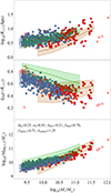 |
Fig. A.1. Same as Fig. 8, but for the best-fit simulation LH_717, obtained by considering the gas mass as a systematic contribution to the simulations’ DM mass. |
Appendix B: Raw parameter constraints
In this section, we show the tables reporting the constraints obtained from the bootstrap procedures without the smoothing of the CDFs.
Constraints on cosmological and astrophysical parameters, obtained by bootstrapping both observational and simulated datasets and taking for each resampling the best-fit simulation.
Constraints on cosmological and astrophysical parameters, obtained by bootstrapping the observational (including SPARC) and simulated datasets, and taking for each resampling the best-fit simulation.
Appendix C: Chi-squared heat maps
A potential issue in the extraction of cosmological and astrophysical parameters from the procedure described in the paper is the presence of degeneracies, which allows for simulations with wildly different parameters to have similar values of chi-squared, thus increasing the uncertainty in the parameters. It is thus useful to study the relation between different cosmological and astrophysical parameters in terms of values of chi-squared. In Fig. C1, we plotted heat maps that show the parameter spaces Ωm-σ8, ASN1-ASN2, AAGN1-AAGN2 and Ωm-ASN1. These planes give complete information about the parameter space, and thus other figures with different combinations would be redundant. The plots are colour-coded with the value, for all pair of points associated to each simulation, of the logarithm of the median of the 100 values of the cumulative  obtained by resampling the respective simulation. Regions of low (high) chi-squared are shown in blue (orange). Each row shows a different observational dataset from which the values of
  were obtained, with the same order as that of Table 5. We avoided reporting the plots for the ETG-only observational datasets to avoid redundancy, given that the plots are very similar to those shown in the first three rows of Fig. C1.
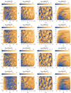 |
Fig. C.1. Heat maps showing regions of the parameter space as a function of the value of cumulative reduced chi-squared for each simulation. The colours show the logarithm of the median of the 100 values of |

From the figure, we deduce that in all cases there is a degeneracy in the Ωm-σ8 plane, which is roughly given by a vertical band. This strong degeneracy along the σ8 axis seems to be associated to the uncertainty in the σ8 parameter estimation. A degeneracy in the ASN1-ASN2 plane is also visible, with an hyperbole-shaped blue region in the lower left corner of the parameter space. This degeneracy seems to constrain either ASN1 or ASN2 to have low values, with the other parameter having a large uncertainty. We cannot detect any degeneracy in the AAGN1-AAGN2 plane, while there is a weak vertical degeneracy in the Ωm-ASN1 plane, which seems to affect mainly the constraints with the MaNGA DynPop LTGs+ETGs sample. In all cases, the best-fit simulation is within 1σ of the bootstrap constraints. There are cases, however, in which the best-fit simulation is on the edge of the 1σ error bar, mostly associated with low constraining power situations, such as with σ8 and both AGN feedback parameters.
Appendix D: Assessing selection bias due to χ2 definition
With the definition of equation (2), the evaluation of the chi-squared is dominated by low-mass simulated galaxies, such as dwarf ellipticals or LTGs, which are much more numerous than high-mass galaxies. Our approach could thus be biased towards simulations that do a better job in reproducing the low-mass end of the scaling relations. To assess whether this asymmetry introduces such a selection bias, we tried to reproduce the results for IllustrisTNG in Paper I by finding the constraints for the cosmological and astrophysical parameters with respect to the observational SPARC sample, this time by eliminating a fraction of LTGs under a threshold value Mthr. = 1010 M⊙ such that the number of LTGs below this threshold value is equal to the number of LTGs above the threshold value. Results show that the discrepancies between the values of the newly constrained parameters and the constraints obtained in Paper I are negligible. We thus conclude that this selection bias does not influence significantly the results of our work.
All Tables
List of spatial, mass and numerical resolution parameters for the simulations with the best resolution (i.e. TNG300-1, TNG100-1, and TNG50-1) two more simulations with the same box side-length of TNG100-1, but worse resolution (i.e. TNG100-2 and TNG100-3, and CAMELS).
Constraints on cosmological and astrophysical parameters, obtained by bootstrapping both observational and simulated datasets, and taking for each resampling the best-fit simulation.
Comparison between the cumulative reduced chi-squared for the fiducial IllustrisTNG 1P_1_0 simulation and the IllustrisTNG best-fit simulation LH_698 from Paper I.
Constraints on cosmological and astrophysical parameters, obtained by bootstrapping the observational (including SPARC and MaNGA DynPop LTGs) and simulated datasets, and taking for each resampling the best-fit simulation.
Constraints on cosmological and astrophysical parameters, obtained by bootstrapping both observational and simulated datasets and taking for each resampling the best-fit simulation.
Constraints on cosmological and astrophysical parameters, obtained by bootstrapping the observational (including SPARC) and simulated datasets, and taking for each resampling the best-fit simulation.
All Figures
|
Fig. 1. Comparison between SPIDER (grey region), ATLAS3D (red region), MaNGA DynPop (orange region) and the theoretical Mtot–M* relation from Moster et al. (2013) (pink region) with IllustrisTNG simulations having differing astrophysical feedback parameters. Each row in the plot corresponds to a different scaling relation, from top to bottom: stellar half-mass radius, R*, 1/2, DM fraction within R*, 1/2, fDM(< R*, 1/2), DM mass within R*, 1/2, MDM, 1/2, and total (virial) mass, Mtot, as a function of stellar mass, M*. Each column shows the effect of varying one of the four astrophysical parameters. The continuous coloured lines associated to the coloured regions represent the 16th, 50th (median) and 84th percentile of the respective observational dataset distributions. The scatter of the Moster et al. (2013) theoretical relation is taken to be the mean of the scatter of the Mtot-M* relation from Posti et al. (2019). |
| In the text | |
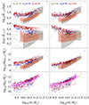 |
Fig. 2. Same as Fig. 1, but considering the cosmological parameters Ωm and σ8. |
| In the text | |
|
Fig. 3. Number of galaxies as a function of the cosmological and astrophysical parameters for each CAMELS IllustrisTNG simulation. Top row shows the number of ETGs, while bottom row shows the number of LTGs. Each column is associated to a different parameter. For each plot, for a fixed value of one of the parameters, the trends with respect to the other parameters are the same as those shown in the other panels. Parameters AAGN1 and AAGN2 are not shown for convenience. |
| In the text | |
|
Fig. 4. Comparison of fiducial IllustrisTNG simulation with observational trends. From top to bottom: stellar half-mass radius, R*, 1/2, DM fraction within R*, 1/2, fDM, and DM mass within R*, 1/2, MDM, 1/2, as a function of stellar mass, M*, for the fiducial IllustrisTNG simulation 1P_1_0, compared with the corresponding SPIDER (black curves), ATLAS3D (dark red curves) and MaNGA DynPop (orange curves) trends. The shaded areas represent the scatter of the observed relations, given by the difference between the 16th and the 84th percentiles with the median. As an example, the open circles are galaxies not used for the evaluation of the cumulative reduced chi-squared associated to the ATLAS3D observational trend in Section 4.2. |
| In the text | |
|
Fig. 5. Same as Fig. 4, but for the best-fit simulation LH_698, found in Paper I to be the best-fit simulation between the simulated LTG data and the SPARC trends. |
| In the text | |
|
Fig. 6. Each column of this figure is the same as in Fig. 4, but for the best-fit simulation associated to SPIDER (left column), ATLAS3D (center column) and MaNGA DynPop (right column) observational trends. Red squares are the simulated galaxies. Filled red squares are for galaxies used for the evaluation of the cumulative reduced chi-squared with respect to the associated observational trend. |
| In the text | |
|
Fig. 7. Same as Fig. 6, but considering both simulated LTGs (blue points) and simulated ETGs (red points). The blue region is the SPARC observational trend from Paper I. |
| In the text | |
|
Fig. 8. Same as Fig. 4, but for the best-fit simulation to the whole MaNGA DynPop sample, LH_531. The blue squares indicate simulated LTG galaxies, while red squares indicate simulated ETG galaxies. The open squares are galaxies not used for the evaluation of the cumulative reduced chi-squared associated to the respective observational trend. The dark orange region is associated to the observed MaNGA DynPop ETG sample, while the green region is associated to the LTG sample. |
| In the text | |
|
Fig. 9. Comparison of different IllustrisTNG suites with observational trends. From top to bottom: stellar half-mass radius, DM fraction within the stellar half-mass radius and DM mass within the stellar half-mass radius as a function of stellar mass, for fiducial CAMELS simulation (first column), TNG-300 (second column), TNG-100 (third column) and TNG-50 (fourth column). The simulated galaxies for all four simulations have been binned in bins of stellar mass (red points for ETGs, blue points for LTGs, uncertainty given by the standard deviation of the y-values in the bins). The coloured regions have the same meaning as in Figs. 1 and 7. |
| In the text | |
|
Fig. A.1. Same as Fig. 8, but for the best-fit simulation LH_717, obtained by considering the gas mass as a systematic contribution to the simulations’ DM mass. |
| In the text | |
|
Fig. C.1. Heat maps showing regions of the parameter space as a function of the value of cumulative reduced chi-squared for each simulation. The colours show the logarithm of the median of the 100 values of |
| In the text | |
Current usage metrics show cumulative count of Article Views (full-text article views including HTML views, PDF and ePub downloads, according to the available data) and Abstracts Views on Vision4Press platform.
Data correspond to usage on the plateform after 2015. The current usage metrics is available 48-96 hours after online publication and is updated daily on week days.
Initial download of the metrics may take a while.