| Issue |
A&A
Volume 693, January 2025
|
|
|---|---|---|
| Article Number | A126 | |
| Number of page(s) | 23 | |
| Section | Extragalactic astronomy | |
| DOI | https://doi.org/10.1051/0004-6361/202451098 | |
| Published online | 13 January 2025 | |
An X-ray study of changing-look active galactic nuclei
1
Dipartimento di Fisica, University di Ferrara, Via Saragat 1, I-44122 Ferrara, Italy
2
Lomonosov Moscow State University/Sternberg Astronomical Institute, Universitetsky Prospect 13, Moscow 119992, Russia
⋆ Corresponding authors; This email address is being protected from spambots. You need JavaScript enabled to view it.
, This email address is being protected from spambots. You need JavaScript enabled to view it.
Received:
13
June
2024
Accepted:
12
November
2024
Abstract
A significant number of changing-look active galactic nuclei (CL AGNs) have been identified to date. In this work, we study what happens to the X-ray spectrum during CL events. We use the example of the nearby CL Seyfert named NGC 1566, which has been observed by Swift, NuSTAR, XMM-Newton, and Suzaku. We applied the Comptonization model to describe the evolution of NGC 1566 X-ray spectra during outbursts and compared these results with the typical behavior of other AGNs to identify some differences and common properties that will ultimately help us better understand the physics of the CL phenomenon. We found that changes in the X-ray properties of NGC 1566 are characterized by a different combination of Sy1 (using 1H 0707–495 as a representative) and Sy2 properties (using NGC 7679 and Mrk 3 as their representatives). At high X-ray luminosities, NGC 1566 exhibits behavior typical of Sy1. At low luminosities, we see a transition of NGC 1566 from Sy1 behavior to an Sy2 pattern. We revealed the saturation of the spectral indices, α, for these four AGNs during outbursts (α1566 ∼ 1.1, α0707 ∼ 2, α7679 ∼ 0.9, and αmrk3 ∼ 0.9) and we determined the masses of the black holes (BHs) in the centers of these AGNs; namely, M0707 ∼ 6.8 × 10⁷ M⊙, M7679 ∼ 8.4 × 10⁶ M⊙, Mmrk3 ∼ 2.2 × 10⁸ M⊙, and M1566 ∼ 2 × 10⁵ M⊙, applying the scaling method. Our spectral analysis shows that the changing-look of NGC 1566 from Sy1.2 to Sy1.9 in 2019 was accompanied by the transition of NGC 1566 to an accretion regime, which is typical for the intermediate and highly soft spectral states of other BHs. We also find that when going from Sy2 to Sy1, the spectrum of NGC 1566 shows an increase in the soft excess accompanied by a decrease in the Comptonized fraction (0.1 < f < 0.5), which is consistent with the typical behavior of BH sources during X-ray outburst decay. Our results strongly suggest that the broad variations in behavior observed among CL, Sy1, and Sy2 AGNs with different X-ray luminosities can be explained by changes in a single variable parameter (e.g., the ratio of the AGN’s X-ray luminosity to its Eddington luminosity), without any need for incorporating additional differences in the Sy AGN parameters (e.g., inclination). Therefore, we find that the distinction between the Sy1, Sy2, and CL-AGN subclasses is effectively blurred.
Key words: galaxies: active / galaxies: individual: 1H 0707–495 / galaxies: individual: NGC 1566 / galaxies: individual: NGC 7679 / galaxies: individual: Mrk 3 / galaxies: Seyfert
© The Authors 2025
 Open Access article, published by EDP Sciences, under the terms of the Creative Commons Attribution License (https://creativecommons.org/licenses/by/4.0), which permits unrestricted use, distribution, and reproduction in any medium, provided the original work is properly cited.
This article is published in open access under the Subscribe to Open model. This email address is being protected from spambots. You need JavaScript enabled to view it. to support open access publication.
1. Introduction
Recent detections of numerous changing-look active galactic nucleus (CL AGN) events have led to a surge of interest in the study of this phenomenon. The origin of the CL-AGN events is still unclear. NGC 1566 is a prominent representative of the CL-AGN subclass of AGNs, with a supermassive black hole (SMBH) estimated to be (1.3 ± 0.6)×107 M⊙. As the closest galaxy (z = 0.005, see also Table 1) among CL-AGNs, NGC 1566 has been studied intensively over the past 70 years. It was first classified as a Seyfert 1 (Sy1) based on broad Hα and Hβ lines (de Vaucouleurs & de Vaucouleurs 1961). The Hβ line was later found to be weak, leading to its classification as a Seyfert 2 (Sy2) galaxy (Pastoriza & Gerola 1970). This is consistent with the generally accepted classification of AGN as Sy1 or Sy2, depending on the presence or absence of broad optical emission lines.
Basic information on 1H 0707–495, NGC 1566, and NGC 7679.
The existence of different classes of AGN can be explained using a unified model (Antonucci 1993) based on the orientation of an optically thick torus relative to the line of our vision. However, NGC 1566 exhibits the appearance or disappearance of broad optical emission lines, transitioning from Sy 2 (or Sy 1.8–1.9) to Sy 1 (or Sy 1.2–1.5) and vice versa within a few months (da Silva et al. 2017). Thus, it does not fit into the generally accepted classification and constitutes a significant problem in our understanding of AGNs.
Since 2018, observations of NGC 1566 have been carried out in many wavelength ranges: from hard X-rays (see X-ray image of NGC 1566 in Fig. 1) to infrared rays (Ducci et al. 2018). It has become clear that the NGC 1566 flux varies in all wavelengths. In particular, in July 2018, its flux increased strongly and reached its peak (Parker et al. 2019; Oknyansky et al. 2019, 2020). The long-term light curves of ASAS-SN and NEOWISE showed that the IR and optical flux began to rise as early as September 2017 (Cutri et al. 2018; Dai et al. 2018). The Swift/XRT flux increased by about 30 times (Fig. 2) when the source changed from Sy1.8–1.9 to Sy1.2 (Oknyansky et al. 2020, 2019). The source became Sy1, with the appearance of strong broad emission lines (Oknyansky et al. 2019; Ochmann et al. 2020). Having reached their peak, the source fluxes decreased in all wavebands. Several smaller flares were observed after the main outburst (Grupe et al. 2018, 2019).
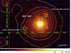 |
Fig. 1. X-ray image of NGC 1566 (in center), accumulated by /XRT from December 12, 2007 to November 2, 2023 with a 230 ks exposure time. The yellow contours in this image demonstrate the lack of X-ray jet-like structure, as well as minimal contamination by other point sources within 18″. The closest next source is 21″(LSXPS J041956.5–545528 is marked with a green circle). |
This 2018–2019 outburst of NGC 1566 with a CL-effect was observed using NuSTAR and XMM-Newton. Jana et al. (2021) investigated these observations applying the power-law, NTHCOMP, OPTXAGNF, and RELXILL models, with the addition of Gaussian lines and taking into account X-ray absorption effects. Each of these models shed light on the CL-peculiarities and the change in the object itself. In the power-law model, Jana et al. (2021) found the presence of a soft excess (< 2 keV), which they approximated by an additional bbody component. This model fits the XMM-Newton data well for about 2.5 years before the 2018 outburst, with the parameter NH = (3.53 ± 0.06)×1021 cm−2 and a photon index of Γ ∼ 1.7 (Γ = α − 1). Moreover, an iron Kα emission line was detected at 6.4 keV with an equivalent width (EW) of 200 eV. The rise phase of the 2018 outburst was analyzed using simultaneous XMM-Newton and NuSTAR observations of NGC 1566. In this model, the fit yielded Γ = 1.8.
The Fe Kα line was detected at 6.38 keV with an EW > 110 eV, as well as the Fe XXVI emission feature at 6.87 keV with an EW < 37 eV. It is interesting to note that two ionized absorbers were required to fit the source spectra in the rise phase: one low-ionization absorber (ξ ∼ 101.7 ± 0.1), with NH, 1 = (8.1 ± 2.2)×1020 cm−2, and one high-ionization absorber (ξ ∼ 104.7 ± 0.4), with NH, 2 = (4.3 ± 0.4)×1021 cm−2.
In the outburst decay phase, the photon index was almost constant (Γ ∼ 1.7), the blackbody temperature was constant kTbb ∼ 110 eV, and the Fe Kα line was detected with EW > 100 eV. Although the column density of the weakly ionizing absorber varied in the range of NH, 1 ∼ (1.2 − 1.3)×1021 cm−2, no highly ionizing absorber was required to fit the spectra during the outburst decay. In addition, a weak reflection hump was detected as an excess of emission at energies 15–40 keV. In the NTHCOMP model, Jana et al. (2021) fixed the seed photon temperature at kTs = 30 eV; again, this is needed to account for two absorption components during the outburst rise and initial decay phases. These authors found that as the corona size Rcor decreased, the plasma electron temperature, kTe, increased from 60 to 100 keV with a nearly constant photon index (Γ = 1.7 − 1.9).
To model this NGC 1566 outburst with OPTXAGNFJana et al. (2021) again accounted for two absorption components during the outburst rise and initial decay phases. The photon index Γ and optical depth τ were kept almost constant at Γ = 1.7 − 1.8 and τ ∼ 4 − 5 throughout the 2018 outburst. Before this outburst, the Eddington ratio and the size of the X-ray corona were found to be small (L/LEdd ∼ 0.04 and Rcor = 12Rg) compared to the rise phase outburst (L/LEdd ∼ 0.23 and Rcor = 43Rg). In later observations, they decreased these values to L/LEdd ∼ 0.06 and Rcor ∼ 20Rg.
This model fit all observations well and indicated an increase in the accretion rate and corona size at the outburst peak, as well as a high degree of the plasma Comptonization during the outburst. The RELXILL model again required taking into account two absorption components during the rising and initial decay phases of the outburst. In addition, the model included the reprocessed X-ray emission from the disk as a reflectivity parameter Rrefl, which turned out to be relatively weak (Rrefl ∼ 0.1 − 0.2) throughout the outburst. The inner disk edge Rin varied from 4Rg to 7Rg.
Tripathi & Dewangan (2022a) (hereafter TD22a) also analyzed NGC 1566 using XMM-Newton, Swift and NuSTAR data at different epochs during the decay phase of the 2018 outburst using a broadband continuum model OPTXAGNF (Done et al. 2012) taking into account the thermal Comptonization (THCOMP) and the reflection (RELXILL) model, as well as investigated the correlations between the accretion disk X-ray emission, soft X-ray excess and the power-law continuum. They argued that at low X-ray flux levels, the source soft X-ray excess was absent and only the disk emission provided seed photons for thermal Comptonization in the corona, while at high flux levels, both the soft X-ray excess and the disk emission were present, providing seed photons for the thermal Comptonization in the corona.
TD22a reported that the X-ray photon index remained constant (Γ ∼ 1.66 − 1.72), although the electron temperature of the corona increased from 22 to 200 keV from June 2018 to August 2019. At the same time, the optical depth of the corona τ decreased from 4 to 0.7, and the scattering fraction increased from 1% to 10%. TD22a interpreted this as an increase in the size of the corona and its heating with a decrease in the mass accretion rate during the decay phase.
Different models are used to study AGN, including those specifically designed for AGNs (assuming a specific structure for AGNs) and generalized models (with a minimum number of specific assumptions). The first of these, for intance, the AGNSED model (Kubota & Done 2018), along with models taking into account the double (warm and hot) corona (Petrucci et al. 2013), consider three zones of AGN X-ray formation: an outer standard disc, an inner warm Comptonizing region (to produce the soft X-ray excess), and a hot corona (see Fig. 10 in Petrucci et al. 2013). Generalized models such as the BMC (Titarchuk et al. 1997; Titarchuk & Zannias 1998; Laurent & Titarchuk 1999; Borozdin et al. 1999; Shrader & Titarchuk 1999), NTHComp (Zdziarski et al. 1996), Comptb (Farinelli & Titarchuk 2011), Comptt (Titarchuk 1994) are based on the first principles and also consider three X-ray formation regions: an outer standard disc, a hot Comptonizing region (a so-called transition layer) to reproduce the soft X-ray excess and a thermal Comptoniziation hump in the source spectrum, along with a converging flow region (possibly analogous to a hot corona, to form a hard high-energy tail in the source X-ray spectrum). In this paper, we apply these generalized models to identify the features of CL-AGN compared to Sy1 and Sy2, without assuming a specific geometry for these sources.
In addition, to better understand the properties of NGC 1566 during CL events, it is interesting to compare the behavior of this CL-AGN with other AGNs, such as Sy1 and Sy2. To do so, we used the Sy1 galaxy (1H 0707–495) and the Sy2 galaxy (NGC 7679) to study their differences and similarities during X-ray outbursts in comparison to CL-AGN.
The narrowline Sy 1 (NLS1) galaxy 1H 0707–495 (z = 0.0411, hereafter 1H 0707; see also Table 1) is a bright NLS1 galaxy (Leighly 1999). The BH mass estimates in 1H 0707 vary over a wide range from 2 × 10⁶ to 107 M⊙ (Zhou & Wang 2005; Kara et al. 2013; Done & Jin 2016). In particular, Zoghbi et al. (2011) assumed that most of the radiation is emitted at ∼2rg and estimated the inner radius and the emissivity index using their spectral fitting. They interpreted the 30 s lag as the light crossing time and estimated a BH mass of MBH ∼ 2 × 10⁶ M⊙, which is consistent with the uncertain mass of this BH quoted in the literature (Zhou & Wang 2005).
NGC 7679 is a barred lenticular galaxy seen face on (Yankulova et al. 2007). It is located at a distance of about 200 million light years from Earth (see also Table 1). It was discovered by Heinrich d’Arrest on September 23, 1864. The nucleus of NGC 7679 turned out to be active and was classified as a Seyfert galaxy. The most common theory for the energy source of Seyfert galaxies is the presence of an accretion disk around a SMBH. NGC 7679 is believed to host a SMBH, with a mass estimated at 5.9 × 10⁶ M⊙ based on velocity dispersion (Alonso-Herrero et al. 2013). The X-ray spectrum of NGC 7679 using BeppoSAX shows no significant absorption above 2 keV and the Kα line of iron was only slightly detected. However, the galaxy shows signs of obstruction to visual light as it lacks broad emission lines. Two possible reasons: the presence of dust or an X-ray emitting accretion disk that is not covered and the broad line region is covered (Risaliti 2002). To date, the classification of NGC 7679 as Sy1 or Sy2 remains controversial. On the one hand, this AGN has an optical spectrum without broad emission lines, which allows it to be classified as a Sy2 (Risaliti 2002). On the other hand, NGC 7679 has significant variable X-ray emission, typical of Sy1. The main feature of objects like NGC 7679 is not the strength of their starburst, but the apparent optical faintness of the Sy1 nucleus when compared to the X-ray luminosity.
As a second representative of Sy2 galaxies we used Markarian 3 (hereafter, Mrk 3), which is one of the brightest and best-studied members of the Sy2 class. The host galaxy is classified as an elliptical or S0 galaxy type. Awaki et al. (1990), Awaki et al. (1991) and Smith & Done (1996) revealed an anomalously flat power-law continuum emerging through a tall occultation column (NH ∼ 6 × 1023 cm−2) from GINGA observations of Mrk 3. A strong Fe line with a high equivalent width (EW ∼ 1.3 keV) was also detected. Mrk 3 has the hardest spectrum among all 16 Sy2 galaxies studied by Smith & Done (1996), significantly harder than the spectrum of Sy1 galaxies. In ASCA observations of Mrk 3, the object showed a spectrum with a photon index Γ ∼ 1.8 and a two-component iron line (Iwasawa et al. 1994).
Thus, the dominant component of the Kα iron line at 6.4 keV has EW = 0.9 keV, while the second component at 7 keV has and EW = 0.2 keV. A reanalysis of the spectrum of Mrk 3 using non-simultaneous GiINGA, ROSAT, and ASCA observations (Griffiths et al. 1998) covering a wide spectral band (0.1–30 keV) yielded a typical value for the power law, Γ ∼ 1.7, when either an additional absorption edge at 8 keV (possibly arising from a warm absorber) or reflection was included in the spectral model. Recent observations with BeppoSAX (Cappi et al. 1999), which extend the spectral coverage to 150 keV, indeed confirm a presence of a steep (Γ∼ 1.8) internal power law. Turner et al. (1997) also reanalyzed the ASCA data and proposed an alternative model in which the internal continuum is resolved through very large absorption column (NH > 1024 cm−2), while the reflection component is not obscured.
Georgantopoulos et al. (1999) analyzed the RXTE data for Mrk 3 and found an agreement with the earlier results of GINGA. They used a spectral model consisting of a very hard power-law continuum (Γ ∼ 1.1) modified below ∼6 keV by a strongly absorbing column (NH ∼ 6 × 1023 cm−2) and an iron line with a high equivalent width at 6.4 keV. Their conclusions are consistent with the results by Turner et al. (1997) on the complex absorption of a molecular torus.
It is interesting to note that Boorman et al. (2018) found an anti-correlation between the equivalence width of the narrow core of the neutral Fe Kα fluorescence line, ubiquitously observed in the reflection spectra of obscured AGNs, and the mid-infrared continuum luminosity at 12 μm. This is consistent with numerous studies of the X-ray Baldwin effect for unobscured and slightly obscured AGNs and challenges the traditional view that the Fe Kα line originates from the same region as the underlying reflection continuum, which together make up the reflection spectrum. However, this anti-correlation does not apply to Mrk 3, as Ricci et al. (2015) have found a Compton-thin column density (90% confidence level) for this source.
Risaliti et al. (2002) discussed another type of X-ray changing look for AGNs based on changes in column density (from 20% to 80%) during AGN X-ray variability on time scales of months to years. Specifically, the AGN switched between thin Compton thin (NH < 1.5 × 1024 cm−2) and Compton thick (NH > 1.5 × 1024 cm−2) regimes (see also Matt et al. 2003).
To describe the BH states in AGN during outbursts, it is convenient to use the terminology used to identify the BH states in X-ray binaries (XRBs). Thus, the observed manifestations of BHs in galactic sources are traditionally described in terms of a classification of BH spectral states (see Klein-Wolt & van der Klis 2008; Remillard & McClintock 2006; Belloni et al. 2005), for various definitions of BH states). A general classification of BH states for four main BH states is accepted by the community: the quiescent, low-hard (LHS), intermediate (IS, sometimes subdivided into hard-intermediate, HIMS, and soft intermediate, SIMS), and the high soft (HSS) states.
When a BH transient goes into an outburst, it leaves the quiescent state and enters the LHS, a low-luminosity state with an energy spectrum dominated by the thermal component of Comptonization combined with a weak thermal component. The photon spectrum in the LHS is thought to be the result of Comptonization (upward scattering) of soft photons, which originated in the relatively weak inner part of the accretion disk, from electrons in the hot surrounding plasma (see, e.g., Sunyaev & Titarchuk 1980). The HSS photon spectrum is characterized by a pronounced thermal component, which is probably a sign of strong radiation emanating from the geometrically thin accretion disk. The IS is a transition state between the LHS and the HSS. At the same time, the subdivision the IS into SIMS and HIMS states reflects the specifics of a BH source at the entrance and exit from the outburst. As for SMBHs in AGNs, despite the different time scale, sizes and sources of accreted matter compared to XRBs, they show a similar pattern of the spectral changes during their outbursts. Therefore, in this work, we use the terminology given above, but we note that there is of course no direct analogy. In addition, the excess soft radiation of AGNs is another component of the Comptonization effect, since the disk temperature of AGNs is much lower.
X-ray spectroscopy is a very powerful tool for shedding light on the CL-AGN relationship, mainly because X-rays are emitted closer to the primary emission source than optical emission lines, which are reprocessed emission from interstellar gas (e.g., Terashima et al. 2009). In this paper, we present the comparative analysis for NGC 1566, 1H 0707–495 and NGC 7679 using the Suzaku, ASCA, Swift, and BeppoSAX observations. In Sect. 2, we present the list of observations used in our data analysis; whereas in Sects. 3.1–3.3, we provide the details of X-ray spectral analysis. We analyze an evolution of the X-ray spectral and timing properties during the state transition in Sect. 3.4. In Sect. 3.5, we present a description of the spectral models used for fitting these data. In Sect. 4, we discuss the main results of the paper. In Sect. 5, we present our final conclusions.
2. Data selection
NGC 1566 was observed by Swift (2007–2023) and with Suzaku (2012), while 1H 0707–495 was detected by Swift (2010–2018) and by ASCA (1995, 1998 and 2005) as well as with Suzaku (2005). NGC 7679 was observed by Swift (2017 and 2019), by ASCA (1998 and 1999), and with BeppoSAX (1998). We extracted these data from the HEASARC archives and found that they cover a wide range of X-ray luminosities (see Tables A.1 and A.2). We recognize that the well-exposed BeppoSAX, ASCA, and Suzaku data are preferable for the determination of low-energy photoelectric absorption.
2.1. Swift data
Using Swift/XRT data in the 0.3–10 keV energy range, we studied flaring events of NGC 1566, 1H 0707, and NGC 7679 (see the log of observations for all three sources in Table A.2). The data used in this paper are public and available through the GSFC public archive1.
The data were processed using the HEASOFT v6.14, the tool xrtpipeline v0.12.84, and the calibration files (CALDB version 4.1). The ancillary response files were created using xrtmkarf v0.6.0 and exposure maps were generated by xrtexpomap v0.2.7. The source events accumulated in a circular region of optimal radius from 17 to 45″ centered on the individual source position shown in Table 1. The background was estimated in a nearby source-free circular region taking into account the relative areas of the source and background regions. Spectra were rebinned with at least ten counts in each energy bin using the grppha task in order to apply χ2 statistics. We also used the online XRT data product generator2 to obtain the image of the source field of view in order to make a visual inspection and to get rid of possible contamination by nearby sources (Evans et al. 2007, 2009).
2.2. BeppoSAX data
We used BeppoSAX data of NGC 7679 carried out on December 6–9, 1998. In Table A.1 (bottom line), we show the log of the BeppoSAX observation analyzed in this paper. Generally, broadband energy spectra of the source were obtained combining data from three BeppoSAX narrow-field instruments (NFIs): the Low Energy Concentrator Spectrometer (LECS; Parmar et al. 1997) for 0.3–4 keV, the Medium Energy Concentrator Spectrometer (MECS; Boella et al. 1997) for 1.8–10 keV and the Phoswich Detection System (PDS; Frontera et al. 1997) for 15–60 keV. The SAXDAS data analysis package is used for processing data. For each of the instruments, we performed the spectral analysis in the energy range for which the response matrix is aptly determined. Both the LECS and MECS spectra were accumulated in circular regions of 4′ radius. The LECS data have been re-normalized based on MECS. Relative normalization of the NFIs were treated as free parameters in the model fitting, except for the MECS normalization that was fixed at a value of 1. We checked after that this fitting procedure whether these normalizations were in a standard range for each instruments3. In addition, the spectra were rebound accordingly, based on energy resolution of the instruments in order to obtain significant data points. We rebinned the LECS spectra with a binning factor, which is not constant over energy (Sect. 3.1.6 of Cookbook for the BeppoSAX NFI spectral analysis), using re-binnig template files in GRPPHA of XSPEC4. Also we re-binned the PDS spectra with linear binning factor 2, grouping two bins together (resulting bin width is 1 keV). Systematic error of 1% have been applied to these analyzed spectra.
2.3. Suzaku data
NGC 1566 and 1H 0707 have been observed by Suzaku. Table A.1 summarizes the start and end times, and the MJD interval for each of these observations, indicated by a green triangle in top of Fig. 2 for NGC 1566. A description of the Suzaku experiment is given in Mitsuda et al. (2007). For observations obtained by a focal X-ray CCD camera, X-ray Imaging Spectrometer (XIS; Koyama et al. 2007), which is sensitive over the 0.3–12 keV range, we used software of the Suzaku data processing pipeline (ver. 2.2.11.22). We carried out the data reduction and analysis following the standard procedure using the HEASOFT software package (version 6.25) and following the Suzaku Data Reduction Guide5. The spectra of the source were extracted using spatial regions within the 3.51′-radius circle centered on the source nominal position (Table 1), while a background was extracted from source-free regions for each XIS module separately.
 |
Fig. 2. Evolution of NGC 1566 during 2007–2023 observations with Swift/XRT (top panel, 0.3–10 keV), Swift/BAT (bottom panel, black points, 15–150 keV), and Swift/UVOT (bottom panel, orange stars, UVW2 band [1600–2300 Å], right axis). The green, black, and red triangles indicate the Suzaku, NuSTAR, and XMM-Newton observations, respectively, used in our analysis. |
The spectrum data were re-binned to provide at least 20 counts per spectral bin to validate the use of the χ2-statistic. We carried out spectral fitting applying XSPEC v12.10.1. The energy ranges around of 1.75 and 2.23 keV are not used for spectral fitting because of the known artificial structures in the XIS spectra around the Si and Au edges. Therefore, for the spectral fits, we have chosen the 0.3–10 keV range for the XISs (excluding 1.75 and 2.23 keV points).
2.4. ASCA data
ASCA observed 1H 0707–495 and NGC 7679 (see Table A.1, which summarizes the start time, end time, and MJD interval). A description of the ASCA data is given in Tanaka et al. (1994). The solid imaging spectrometers (SIS) operated in Faint CCD-2 mode. The ASCA data were screened using the ftool ascascreen and the standard screening criteria. The spectrum for the source were extracted using spatial regions with a diameter of 4′ (for SISs) and 6′ (for GISs) centered on the nominal position of the source, while the background was extracted from source-free regions of comparable size away from the source. The spectrum data were re-binned to provide at least 20 counts per spectral bin to validate the use of the χ2-statistic. The SIS and GIS data were fitted using XSPEC in the energy ranges of 0.6–10 keV and 0.8–10 keV, where the spectral responses are well known.
2.5. RXTE data
We also analyzed the available data of 1H 0707–495 (1997) obtained with RXTE (Bradt et al. 1993). We carried out an analysis of the RXTE observation of 1H 0707 during the low-hard state (LHS; ID = 20309-01-01-00). We should note that that the LHS and HSS notations are not often applied to AGNs. Altogether, we introduce these notations because of the photon index change Γ. For example, similarly to the case of binary systems, if the Γ index is within the 1.5–1.7 range, then we associate it with the Comptonization photon index, which is typical for the low-hard spectrum in the binaries; vice versa, if Γ > 2.3, then we relate it to the high-soft state (HSS) observed in the binaries.
Standard tasks of the LHEASOFT/FTOOLS 6.33.2 software package were utilized for data processing using methods recommended by RXTE Guest Observer Facility according to the RXTE Cook Book6. For spectral analysis, we used data from the Proportional Counter Array (PCA) and High-Energy X-Ray Timing Experiment (HEXTE) detectors. RXTE/PCA spectra (standard 2 mode data, 3–50 keV energy range) have been extracted and analyzed using the PCA response calibration (ftool pcarmf v11.1). The relevant dead-time corrections to energy spectra have been applied. In turn, HEXTE data in the 20–150 keV energy range were used for the spectral analysis in order to exclude the channels with largest uncertainties. We subtracted the background corrections in off-source observations.
We used the data available through the GSFC public archive7. In Table A.1, we present the informations of the RXTE observation of 1H 0707 and Mrk 3. A systematic error of 0.5% has been applied to the analyzed spectrum.
2.6. NuSTAR data
We processed NuSTAR observations using the NuSTARDAS (version 2.1.1) and the latest files available in the NuSTAR Calibration Database8. We generated clean event files for each observation of NGC 1566 using the nupipeline task and extracted the source and background spectra from circular regions of 60″ and 90″ radius, respectively, centered at the source position (Table 1). Source spectra were extracted using the nuproduct task. We binned each spectrum so that there were at least 25 counts per spectral bin.
2.7. XMM–Newton data
We processed the XMM-Newton data from EPIC-pn (Struder et al. 2001) using SAS software (version 18.0.0)9 and the latest calibration files. Following Jana et al. (2021), we corrected for the pile-up by excluding events in the inner 10″ radius circular region from the clean event lists. We extracted the source spectrum from the annular region (with outer radius 30″ and inner radius 10″10) centered at the source position (Table 1) and the background spectrum from a 40″ radius circular region from the source-free region for each observation. The response files (arf and rmf files) were generated using the SAS arfgen and rmfgen tasks, respectively. We binned each spectrum so that there were at least 25 counts per spectral bin.
3. Results
3.1. Images of NGC 1566, 1H 0707–495, NGC 7679 and Mrk 3
The Swift/XRT (0.3–10 keV) image of the NGC 1566, 1H 0707–495, Mrk 3 and NGC 7679 fields of view (FOVs) are presented in Figs. 1–5, respectively. Swift X-ray image of NGC 1566 (Fig. 1) is accumulated from December 12, 2007 to 1 November 2023 with an exposure time of 230 ks. Yellow contours in this image demonstrate the lack of X-ray jet structure (elongated), as well as minimal contamination by other point sources within 18″ in the field of view around NGC 1566. The closest next source is 21″ (LSXPS J041956.5–545528 is marked with a green circle).
The field of view for 1H 0707 is shown in Fig. 3. Swift X-ray image of 1H 0707–495 (2SXPS J070841.4–493306 – according to the Swift catalog), accumulated from April 3, 2010 to April 30, 2018 with a 161 ks exposure time. The dashed gray square with a side of 6.3′ (160 pixels) in the 1H 0707 image demonstrates the absence of other nearby objects in the 1.3′ field of view. The next closest source is 2.8′ away (outside the image).
 |
Fig. 3. X-ray image of 1H 0707–495 (2SXPS J070841.4-493306 – according to the Swift catalog), accumulated from April 3, 2010 to April 30, 2018 with a 160 ks exposure time. The dashed square with a side of 6.3′ (160 pixels) in the SDSS J0752 image demonstrates the absence of other nearby objects in the 1.3′ field of view. The next closest source is 166″ away (outside the image). |
According to the Swift catalog), the field of view for Mrk 3 is shown in Fig. 4. Swift X-ray image of Mrk 3 (2SXPS J061536.2+710214 accumulated from May 3, 2006 to April 20, 2015-04-20 with a 91 ks exposure time. The green contours in this image demonstrate the lack of X-ray jet-like structure around Mrk 3, as well as minimal contamination by other point sources within 18″ of the source environment. The closest next source is 21″ (LSXPS J041956.5–545528 is marked with a white circle, see Fig. 4).
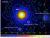 |
Fig. 4. X-ray image of Mrk 3 (in center), accumulated by Swift/XRT from March 21, 2006 to April 20, 2015 with a 91 ks exposure time. The green contours in this image demonstrate the lack of X-ray jet-like structure around Mrk 3, as well as minimal contamination by other point sources within 18″ of the source environment. The closest next source is 21″ (LSXPS J041956.5–545528 is marked with a white circle). |
The Swift X-ray image of NGC 7679, presented in Fig. 5, is catalog), accumulated from July 25, 2015 to October 6, 2017, with a 1.7 ks exposure time. The image segment highlighted with a gray square (6.3′ to a side) is also shown in more detail in the enlarged panel. Contour levels demonstrate the absence of X-ray jet (elongated) structure and minimal contamination from other point sources and diffuse radiation in the 1.3′ field of view around NGC 7679. The next closest source (at 279″ is 2LSXPS J232904+032910.
 |
Fig. 5. X-ray image of NGC 7679 (LSXPS J232846.7+033042 – according to the Swift catalog), accumulated from July 25, 2015 to October 6, 2017 with a 1.7 ks exposure time. The image segment highlighted with a gray square with a side of 6.3′ (160 pixels) is also shown in more detail in the enlarged panel. Contour levels demonstrate the absence of X-ray jet (elongated) structure and minimal contamination from other point sources and diffuse radiation in the 1.3′ field of view around NGC 7679. The next closest source is 2LSXPS J232904+032910, 279″ away. |
3.2. X-ray light curves
All three sources are Seyfert galaxies and the BHs at their centers have approximately the same masses (∼106 M⊙, see Table 1). However, they exhibit completely different temporal patterns of activity. To demonstrate this, we compared their long-term behavior in the form of light curves.
3.2.1. NGC 1566 light curve
We present a long-term X-ray light curve of NGC 1566 detected by the XRT on board Swift between 2007–2023 (see Fig. 2). In addition, we used Suzaku data from this AGN and marked the time of its observations with a green arrow in the background of the Swift light curve (top panel). At the bottom panel of this figure, we present the optical light curve by Swift/UVW2 [1600–2230 Å] (hazel stars) and by Swift/BAT [15–50 keV] (black dots) observations to trace the quiet and active states of NGC 1566 at different wavelengths. Figure 2 also shows that NGC 1566 was in the LHS state from 2007 to 2017.
Here, along with the count-rate light curve in total band [0.3–10 keV], it is also interesting to investigate the hardness count-rate light curves without using any model. Thus, we study the light curve of NGC 1566 with a bin time of 1 ks for four energy bands 0.3–10 keV, 0.3–1 keV, 1–2 keV, and 3–10 keV. Using these energy-dependent light curves, the soft hardness coefficient (HR1) is defined as the ratio of the difference in count rates in the 1–2 keV (M) and 0.3–1 keV (S) energy bands to their sum, while the hardness coefficient (HR2) is defined as the ratio of the difference in count rates in the 2–10 keV (H) and 1–2 keV (M) energy bands to their sum (see recommendations in 2SXPS11): HR1 = (M − S)/(M + S) and HR2 = (H − M)/(H + M). In this approach, NGC 1566 shows variability in terms of HR1 (blue points) and HR2 (pink points) during transient events from 2007 to 2023 (see second panel from top in Fig. 6). From 2017 to 2019, the object entered an active state with a powerful outburst, followed by decay, accompanied by a series of repeated re-flares of smaller amplitude. Comparison of the top and bottom panels of Fig. 6 demonstrate that the source light curves in the optical (UVW2) and X-ray (Swift/XRT and Swift/BAT) ranges correlate quite well. Around this time a changing-look of the galaxy occurred. It can be seen that during the changing-look events (marked by vertical blue stripes, F1 − F4) NGC 1566 was characterized by the dominance of the soft component, and only after the outburst peak, a softening of its spectrum occurred during repeated small flares (MJD 58400–59000, F2 − F3) during the decay phase. Thus, this interval is most interesting for subsequent spectral analysis (see Sect. 3.3).
 |
Fig. 6. Evolution of the Swift/XRT count rate, hardness ratios HR1 and HR2 (blue and crimson points, respectively), Comptonized fraction f, and BMC normalization during 2007 and 2023 flare transition of NGC 1566 (shown from top to bottom). In the very bottom panel, we present an evolution of the photon index Γ = α + 1. The decay phases of the flares are marked with blue vertical strips. The peak outburst times are indicated by the arrows at the top of the plot. For the three bottom panels, NuSTAR and XMM-Newton observations are indicated with stars and circle points, respectively. |
3.2.2. 1H 0707 light curve
The light curve of Sy1 galaxy 1H 0707 is shown in Fig. 7 before, during, and after the transient events from 2010 to 2018. It can be seen that in 2011 (MJD 55550–65599), 1H 0707 remained in the stable low-hard state (mean count rate ∼0.02 cnt/s). During the rest of the Swift observations, the object is highly variable.
 |
Fig. 7. Evolution of the Swift/XRT count rate during 1996–2010 observations of 1H 0707–495. |
Overall, 1H 0707 shows four X-ray outbursts (marked with vertical blue strips) with a good coverage of the rise-peak-decay in our sample (see Table A.2). Furthermore, the object shows variability in terms of HR1 (blue dots) and HR2 (pink dots) during transient events, with a clear dominance of source hard emission from 2010 to 2018 (Fig. 8).
 |
Fig. 8. Evolution of the Swift/XRT count rate, hardness ratios HR1 and HR2 shown as blue and crimson points, respectively, along with the Comptonized fractionm f, and BMC normalization during 2010–2018 flare of 1H 0707 (from top to bottom). In the very bottom panel, we present an evolution of the photon index Γ = α + 1. The decay phases of the flares are marked with blue vertical strips. |
3.2.3. NGC 7679 light curve
The Sy2 galaxy NGC 7679 has a modest monitoring history and, according to optical observations (see Fig. 9 from Catalina Sky Survey (CSS, V-band, blue dots), the object is weakly variable, at least in the V band. In Fig. 9, we also show the time distribution of observations of NGC 7679 using ASCA (grey arrows), BeppoSAX (green arrow), and Swift/XRT (bright blue vertical strip with red points) in conjunction with the source optical light curve in V band. Apparently, Swift/XRT detected an X-ray flare from NGC 7679 around MJD 58033.
 |
Fig. 9. Distribution of NGC 7679 observations by Swift/XRT (bright blue vertical strip with red points), BeppoSAX (green arrow), and ASCA (grey arrows) is shown along with the CSS V-band light curve (blue points). See Tables A.1 and A.2 for more details. |
3.2.4. Mrk 3 Light Curve
The light curve of Sy2 galaxy Mrk 3 is shown in Fig. 10 before, during, and after the transient events from 2010 to 2018. From this figure, we can see that in early 1996 (MJD 50450–50520), Mrk 3 remained in a stable low-hard state (average count rate of ∼2 − 3 cnt/s). Then two outbursts occurred around MJD 50540 and 50550, when the count rate increased to 5 cnt/s. During the rest of the RXTE observations the object remained in a stable low-hard state.
 |
Fig. 10. Evolution of the RXTE/PCA count rate, fluxes in 3–10 keV (blue points), and 10–20 keV (crimson points) bands, Comptonized fraction, f, and BMC normalization during 1997–1997 flare events of Mrk 3 (from top to bottom). In the very bottom panel, we present an evolution of the photon index Γ = α + 1. The decay phases of the flares are marked with blue vertical strips. |
Generally, Mrk 3 shows two X-ray outbursts (marked with vertical blue strips) in our sample (see Table A.1). Furthermore, the object shows variability in X-ray fluxes in 3–10 keV (blue dots) and 10–20 keV (pink dots) bands during transient events with a clear dominance of source hard emission from 1996 to 1997 (Fig. 8).
3.3. Spectral analysis
3.3.1. Model selection
Special approaches such as AGNSED (Kubota & Done 2018) and dual-coronal methods (Petrucci et al. 2013) have been undertaken to model AGN spectra . In fact, they take into account the specific geometry of AGNs with a breakdown into an outer standard disc, an inner warm Comptonization region, and a hot corona (Kubota & Done 2018). The last two components are called warm and hot corona (dual-coronal model by Petrucci et al. 2013), which are described by the thermal Comptonization with different plasma temperatures. Petrucci et al. used mainly the warm corona component to describe the soft X-ray excess in the AGN spectra in the low-hard state (also see the discussion in Sect. 4).
Titarchuk (1994, 2010), Titarchuk et al. (2020, 2014, 2023, 1997), Titarchuk & Seifina (2021, 2023, 2009, 2016a,b, 2017, 2024), Titarchuk & Zannias (1998) in their papers indicate that the generalized Comptonization model called XSPEC BMC (bulk motion Comptonization is a XSPEC Comptonization by relativistic matter model12) can be applied to any state and Comptonization type (thermal or dynamic) for the observed X-ray spectra of BHs or NSs (Titarchuk & Seifina 2024, 2023, 2021, 2017, 2016a, 2016b, 2009; Titarchuk et al. 2020, 2023, 2014, 2010). Thus, we applied the BMC model as a generalized one for all AGN sources in all spectral states.
The BMC model calculates the soft excess and the primordial emission self-consistently. In this model, the total emission is determined by the BMC normalization, Nbmc, which is proportional to the mass accretion rate and the spectral index α (or the photon index Γ = α + 1). The disk emission appears as a color temperature-corrected blackbody emission at radii Rout > r > RTL, where Rout and RTL are the outer disk radius and the outer radius of the transition layer (TL), respectively. At r < RTL, the disk emission appears as the Comptonized emission from the warm and optically thick medium, rather than as the thermal one. The hot and optically thin TL is located in the inner part of the disk around the BH (RTL < r < RISCO, where RISCO is the radius of the last stable orbit) and creates a high-energy power-law continuum. The total Comptonized radiation is split between the (hot) TL and the (cold) BH-converging flux (CF, where dynamical Comptonization is effective), and the fraction of (hot) Comptonized radiation (f or log A) can be found from a model fit. The seed photon temperature (kTs) and the TL spectral index of the corona determine the energy of the upward-scattered soft excess radiation. The Compton continuum is approximated as a convolution of the BB blackbody radiation, with the Comptonization Green function, G, which can be described as
 (1)
(1)
 (2)
(2)
where x = hv/kTe, x0 is the breakpoint of G(x, x0) at the point where the two cases (x > x0 and x < x0) meet each other. Thus, the general model consists of a BBody-like and a Comptonized component (XSPEC models BMC, COMPTB, and COMPTT are the sum of these components: BB + f ⋅ BB * G). When using the BMC model, we included a Gaussian component to account for the Fe emission lines. As a result, the spectral model in XSPEC terms is tbabs * (BMC+Gaussian). For all sources, we used the Comptonization model BMC modified (see the description of the model in Fig. 11) by neutral absorption and the Gaussian line at ∼6.5 keV. The parameters of a Gaussian component are a centroid line energy, Eline, the width of the line, σline, and normalization, Nline, to fit the data in the 6–8 keV energy range. We also used an interstellar absorption with a column density of NH (see Table 1).
 |
Fig. 11. A suggested geometry for NGC 1566, 1H 0707, Mrk 3 and NGC 7679 sources. Disk soft photons are upscattered (Comptonized) off of the relatively hot plasma of the transition layer. |
As for the inclusion of the iron line in the source spectrum fitting model for 1H 0707, some explanations should be given here. The first time the iron fluorescent line in 1H 0707–495 was detected by Fabian et al. (2009) using XMM-Newton. The previous observations showed only a sharp and deep drop in the spectrum at 7 keV, but did not reveal narrow emission features. This has given rise to two interpretations (Boller et al. 2002): either the source is partially shielded by a large layer of iron-rich material (then the sharp drop is due to a photoelectric absorption edge) or it has very strong X-ray reflection (Fabian et al. 2004) in its innermost regions, where relativistic effects change the observed spectrum (the sharp drop in the spectrum by energy 7 keV is due to the blue wing of the line see also Seifina 1999, partly formed by relativistic Doppler shifts).
Absorption requires the iron abundance to be about 30 times the solar value, while reflection requires this ratio to be between 5 and 10. Fabian et al. (2009) showed that the extreme variability in the soft range of the 1H 0707 spectrum does not make sense in the model partial coverage. However, an analysis of the spectral variability of the source showed the spectrum of the source in all states (low and high flux) to be well described by a power-law continuum with a photon index Γ = 3, with an excess at lower energies (≤1.1 keV). Fabian et al. (2009) argued that the 1H 0707 spectra are well described by a simple phenomenological model consisting of a power-law continuum, a soft blackbody, two relativistically broad Laor lines (Laor 1991), and galactic absorption (corresponding to NH = 5 × 1020 cm−2). These lines are characterized by energies of 0.89 and 6.41 keV (in the rest frame), an innermost radius of 1.3Rg (Rg = GMBH/c2, wherein G and c as the common physical constants and MBH as a BH mass), an outer radius of 400Rg, an emissivity of 4, and an inclination of 55.7 degrees. The rest energies of these lines correspond to ionized iron-L and K, respectively. However, Fabian et al. (2009) found the iron abundance to be almost nine times of the solar value, which they associated with the possible influence of a dense nuclear star cluster in the vicinity of 1H 0707. This could lead to the formation of massive double white dwarfs that enriched the core with iron-rich supernova emissions (Shara & Hurley 2002).
In the present paper, we make the assumption that this shape of the ionized iron-K line in the 1H 0707 spectrum may be due to the outflowing wind; to a first approximation, this can be described by an iron line with a Laor profile. The presence of outflowing gas from the nuclear environment of 1H 0707 is supported by recent near-infrared spectroscopy in the zJHK bands, which revealed the dominance of broadband lines at low ionization. In particular, extensive components in H I, Fe II, and O I were found, shifted at a velocity of ∼500 km/s. At the same time, most lines have a blue-asymmetric profile, the velocity shift of which is ∼826 km/s. This feature is consistent with previous indications of escape gas in 1H 0707, observed in the X-ray and UV lines and now found in the low ionization lines. Rodriguez-Ardila et al. (2024) argue that the wind can propagate far into the region of the narrow line due to the observation of a blue-shifted component in the forbidden [S III] λ9531 Å line. Xu et al. (2021) revealed absorption edges in the fits of the 1H 0707 spectra, which can also be interpreted as evidence of a clumpy, multi-temperature outflow around 1H 0707. Therefore, to describe the 1H 0707 spectra, we used tbabs*(bmc+N×Laor). The Laor model parameters are the line energy, EL, the emissivity index, a dimensionless inner disk radius, rin = Rin/Rg, inclination, i, and the normalization of the line, NL (in units of photons cm−2s−1).
For the Laor component, we fixed the outer disk radius to the default value of 400 Rg and varied all other parameters. We also fixed the emissivity index to 3. The inclination is constrained to a value i ∼ 50°. As a result, in our spectral data analysis for all three sources we use a model which consists a sum of a Comptonization component (BMC) and Gaussian (Laor) line component for NGC 1566 and NGC 7679 (1H 0707). We recall here that the BMC spectral component has the following parameters: the seed photon temperature, Ts, the energy index of the Comptonization spectrum, α (=Γ − 1), a Comptonization fraction, f [f = A/(1 + A)], which is the relative weight of the Comptonization component, and normalization of the seed photon spectrum, Ncom. When the parameter log(A) = ≫ 1, we fixed log(A) = 2 because the Comptonized illumination fraction f = A/(1 + A)→1 and varying A no longer improves the fit quality.
3.3.2. NGC 1566 spectra
A spectral analysis of the NGC 1566 observations by Suzaku and Swift indicates that the source spectra can be reproduced by a model with an absorbed Comptonization component, the XSPEC BMC model13 with the addition of a Gaussian iron line component. In Figs. 12 and 14, we present examples of X-ray spectra of NGC 1566 indicating the spectral components in the range 0.3–10 keV and their evolution.
 |
Fig. 12. Four representative spectra of NGC 1566 from Swift data in units of E * F(E) with the best-fit modeling for the LHS (ID = 00014916001 in panel a) IS (ID = 707002010, IS (ID = 00014923002 in panel c), and IS (ID = 00035880003 in panel d) states. The spectrum of NGC 1566 from Suzanne with the best-fit modeling for the LHS (ID = 707002010 in panel b). The data are denoted by crosses, while the spectral model is shown by a red histograms for each state. Bottom: Δχ vs photon energy in keV. |
In the LHS, represented by the Swift observation (ID = 00014916001), the spectrum of NGC 1566 is dominated by the hard emission component (Fig. 12, panel a), which is well reproduced by the Comptonization model with parameters: Γ = 1.40 ± 0.02 and Ts = 110 ± 12 eV (reduced χ2 = 0.95 for 563 d.o.f). With better energy resolution in the LHS state, the spectrum of NGC 1566 with the Suzaku observation is also well described by the Comptonization component, but with an addition of a noticeable emission feature in the energy range ∼6.4–7.0 keV associated with neutral, H-like and He-like Kα Fe lines (panel b, ID = 707002010). The best-fit model parameters are Γ = 1.77 ± 0.04, Ts = 130 ± 1 eV and Eline = 6.36±0.04 keV (reduced χ2 = 0.95 for 563 d.o.f). In the intermediate state of NGC 1566 (ID = 00014923002 in panel c) the best-fit model parameters are Γ = 2.01 ± 0.04 and Ts = 118 ± 5 eV (reduced χ2 = 0.95 for 86 d.o.f). In panel d, we present again the IS spectrum (ID = 00035880003) in the HSS, for which the best-fit model parameters are Γ = 2.1 ± 0.1, Ts = 90 ± 10 eV (reduced χ2 = 0.99 for 86 d.o.f). The data are presented by black crosses and the best-fit spectral model tbabs*(BMC+Gauss) by the red line. Bottom panels shows Δχ versus the photon energy in keV (see more details in Table 2). In the bottom panels, we present Δχ versus the photon energy in keV.
Best-fit parameters for the spectral analysis of ASCA, Suzaku (shaded in gray), BeppoSAX (shaded in blue), NuSTAR (shaded in red), RXTE (shaded in green), and XMM-Newton (shaded in yellow) AGN observations.
We clearly see that the change in spectral state from LHS to HSS in NGC 1566 is accompanied by a slight change in the seed photon temperature, Ts, between 90 and 130 eV, along with an increase in the Γ index from 1.1 to 2.1 (Fig. 13). In details, a number of X-ray spectral transitions of NGC 1566 have been detected by Swift during 2007–2023. We have searched for common spectral and timing features that can be revealed during these spectral transition events. The X-ray light curve of NGC 1566 shows complex behavior in a wide range of timescales: from hours to years (e.g., Oknyansky et al. 2020, 2019). Here we discuss the source variability on timescales of hours. In Fig. 6, we demonstrate the model parameter evolution for all analyzed outburst spectral transitions. As we can see from the HR panel (second from the top), all outbursts of NGC 1566 are characterized by a significant increase in the soft component (HR1, blue points). Some events also demonstrate an increase in the hard component (HR2, pink points) in the decay outburst phase (see particular events at MJD 57000 and 58400–59000).
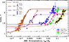 |
Fig. 13. Scaling of photon index Γ for NGC 1566 (with brown line for target source) and NGC 7679 (with violet line for target source) with NGC 4051, GX 339–4, GRO J1655–40, Cyg X–1, and 4U 1543–47 (as reference sources). |
We paid special attention to the flaring events of 2018–2019 (see Fig. 6). Following the terminology of the astronomical community, which previously discussed the changing-look in NGC 1566, we have identified four events F1, F2, F3, and F4 that occurred after the main flare of 2018 (it was not observed using Swift). They are indicated in Fig. 6, using the pink arrows on top of the figure. Event F1 occurred in December 2018 (Grupe et al. 2018), event F2 occurred at the end of May 2019 (Grupe et al. 2019), event F3 occurred in August 2019 (Oknyansky et al. 2020), and event F4 in May 2020 (Jana et al. 2021).
The 2018 outburst itself began in March 2018 (58 200 MJD) according to the V-band ASSAS-SN and Master data (Oknyansky et al. 2019) data. Swift/XRT detected this outburst just a few months later, on June 24, 2018 (MJD 58293.7), when the X-ray intensity increased to 30 times its quiescent state (see Fig. 6). For this outburst with a good peak-decay coverage, the enhancement of the soft component (pink points in the second panel from the top) during the decay phase (Fig. 6, MJD 58452–58749) is correlated with the disappearance of broad lines and [Fe X] λ 6374 Å to 58 561 in the optical spectrum of NGC 1566 (Oknyansky et al. 2020). This may be due to an increase in the illumination of the accretion disk by soft X-rays. We can also suggest that the NGC 1566 spectral state evolution can be traced by the illumination fraction, f. In fact, the parameter f increased greatly during these days (0.7 < f < 1). The photon index Γ is well traced by soft X-ray flux (compare the bottom and two upper panels of Fig. 6). In addition, this may be related to the moderate mass accretion rate regime. In fact, the BMC normalization parameter (Ncom) and photon index (Γ) for these dates are somewhat lower (MJD 58452–58749) than for events at the peak of the 2018 outburst (MJD 58293).
3.3.3. 1H 0707–495 spectra
A spectral analysis of 1H 0707 observations by Suzaku, ASCA, Swift, and RXTE indicates that source spectra can be reproduced by a model with a Comptonization component, the XSPEC BMC model. In Figs. 14 and 15, we present examples of X-ray spectra of 1H 0707 indicating the spectral components in the range 0.3–10 keV and their evolution. The BMC model provides a description of the X-ray emission from the source, which is processed by the accretion disk and/or the surrounding wind environment, with the disk producing the observed Kα iron fluorescence lines, and hump in the continuum. It is clearly seen that the energy range ∼6.4–7.0 keV is also modified by other lines associated with neutral, H-like, and He-like Kα Fe lines. We found a number of positive excesses in the spectrum and added a number of additional lines to better describe the spectrum. Using this approach, we found lines at energies of 6.4, 6.8, 2.9, 1.02, 0.85, 0.65, and 0.5 keV; these are easily associated with Fe I–XXII, Fe XXV/Fe XXVI Kα, lines S XVI, Ne X, Fe XVII, O III and N XVII, respectively.
 |
Fig. 14. Representative E * F(E) spectral diagrams that are related to different spectral states for 1H 0707–495 (top left) using Suzaku observation 00091623 (black, LHS) combined with RXTE/HEXTE observation 20309010100 (black, LHS), ASCA observations 73043000 (bright blue, IS), 73043000 (pink, IS), 763100 (green, IS), Swift observation 0090393 (red, IS) and Swift obs 0091623 (blue, HSS); NGC 1566 (bottom left) using Swift observations 0001496 (blue, LHS), 00014923 (green, LHS), 00031742 (black, IS), 00035880 (red, IS), and NuSTAR observations 80301601002 (pink, IS), 80401601002 (bright blue, IS), 80502606002 (brown, IS), 60501031004 (yellow, IS) and 60501031006 (#bbb7ba;, IS); NGC 7679 (top right) using 40631001 (black, LHS, from BeppoSAX), 00088108002 (#bbb7ba;, LHS, from Swift), 66019010 (red, HIMS, from ASCA), and 66019000 (green, IS, from ASCA) and Mrk 3 (bottom-right) using ASCA observation 70002000 (LHS, red), 70002000 (LHS, red), Suzaku observation 709022010 (LHS, green), RXTE observation 20330-01-09-00 (blue, IS), and BeppoSAX observation 50132002 (IS, black). |
 |
Fig. 15. Best-fit spectrum of 1H 0707–495 in E * F(E) units during: (a) LHS using Suzaku observation 00091623; (b) (IS) using Swift observation 00091623002; (c) IS using ASCA observation 73043000; and (d) HSS using Swift observation 00080720048. The data are presented by crosses and the best-fit spectral model tbabs*(BMC+N*Laor) by red line. The Comptonization hump component is shown by the dotted sea-green line. To model the Laor line components, we used the N XVII (blue), O III (green), Fe XVII (bright blue), Ne X (pink), S XVI (orange), Fe I–XXII, and Fe XXV/Fe XXVI Kα (yellow) lines with energies of 0.5, 0.65, 0.85, 1.02, 2.9, 6.4, and 6.8 keV, respectively. Bottom: Δχ vs photon energy in keV. |
In panel (a) of Fig. 15, we display the best-fit Suzaku spectrum of 1H 0707, which is a typical for the LHS using our model for observation ID = 00091623 carried out on December 3–6, 2005. The best-fit model parameters are Γ = 1.79 ± 0.13, Ts = 121 ± 4 eV, and Eline = 0.83 ± 0.02 keV (reduced χ2 = 1.00 for 802 d.o.f). In panels (b) and (c) of this figure, we present the source spectra for the IS using the Swift observation (ID = 00091623002 and observation ASCA ID = 73043000). The best-fit model parameters for ID = 00091623002 are Γ = 2.00 ± 0.10, Ts = 120 ± 5 eV, and Eline = 0.85 ± 0.08 keV (reduced χ2 = 1.06 for 189 d.o.f). The best-fit model parameters for ID = 73043000 are Γ = 2.03 ± 0.09, Ts = 107 ± 4 eV and Eline = 0.83 ± 0.09 keV (reduced χ2 = 1.01 for 86 d.o.f).
Finally, in panel (d), we show the spectrum of 1H 0707 in the HSS using observation Swift ID = 00080720048, for which the best-fit model parameters are Γ = 2.9 ± 0.1, Ts = 230 ± 10 eV, and Eline = 0.86 ± 0.09 keV (reduced χ2 = 0.97 for 158 d.o.f). The data are represented by black crosses and the best-fit spectral model tbabs*(BMC+N*Laor) by red line. Bottom panels shows Δχ versus photon energy in keV (see more details in Table 2). Thus, we clearly see that the change in spectral state from the LHS to the HSS in 1H 0707 is accompanied by a slight change of the seed photon temperature Ts between 100 and 230 eV and an increase in the Γ index from 1.1 to 2.9 (Fig. 16). For the LHS, we combined the Suzaku and RXTE observations (see Table A.1) to demonstrate that the source spectrum varies over a wide energy range from 0.3 to 200 keV (Fig. 14). In this case, there is a clear dominance of the hard (10–100 keV) emission of 1H 0707 with a slight excess of the soft component at 0.3–2 keV.
 |
Fig. 16. Scaling of photon index Γ for 1H 0707–495 (with black line for target source) and SDSS J0752, OJ 287, and M101 ULX–1 (as reference sources). |
3.3.4. NGC 7679 spectra
In Fig. 17, we show three representative spectra of NGC 7679 for the LHS, HIMS, and IS. We again simulate the spectra using the plasma Comptonization process (BMC), with the addition of a Gaussian iron line component. The best-fit modeling of the NGC 7679 spectrum in the LHS is presented on the left panel using from BeppoSAX data (ID = 40631001) in units of E * F(E). The broadband spectrum [0.3–200 keV] demonstrates a hard tail and has the best-fit parameters: Γ = 1.60 ± 0.02, Ts = 350 ± 60 eV, and Eline = 6.4 ± 0.5 keV (reduced χ2 = 1.04 for 82 d.o.f). In the central panel of this figure, we present the source spectra which are typical for the hard intermediate state (HIMS) using ASCA observation (ID = 66019000). The best-fit parameters are Γ = 1.62 ± 0.02, Ts = 150 ± 70 eV, and Eline = 6.5 ± 0.1 keV (reduced χ2 = 1.09 for 145 d.o.f). Finally, in the right panel, we present the IS spectrum (ID = 00088108002) of NGC 7679 observed by Swift/XRT. The best-fit model parameters are Γ = 1.93 ± 0.07 and Ts = 226 ± 9 eV (reduced χ2 = 0.97 for 194 d.o.f). The data are denoted by crosses, while the red and pink lines stand for the BMC and Gaussian components, respectively. The bottom panels show Δχ versus photon energy in keV.
 |
Fig. 17. Three representative spectra of NGC 7679 with the best-fit modeling for the LHS (ID = 40631001, left) using the BeppoSAX data, HIMS (ID = 66019000, center) from ASCA and for the IS (ID = 00088108002, right) from Swift in units of E * F(E) using the tbabs*(bmc+gauss) model, respectively. The data are denoted by crosses, while the spectral model is shown by a red histograms for each state. o model the line component, we used Fe XXV/Fe XXVI Kα (pink) lines with energies of 6.7/6.9 keV. Bottom: Δχ vs photon energy in keV. |
3.3.5. Mrk 3 spectra
In Fig. 18, we show four representative spectra of Mrk 3 for the LHS and IS states. We simulates these spectra using the BMC model with the addition of a Gaussian iron line component. The best-fit model of the Mrk 3 spectrum of the LHS is presented in panel (a) using from ASCA data (ID = 70002000) in units of E * F(E). The best-fit parameters are Γ = 1.102 ± 0.02, Ts = 180 ± 10 eV, and Eline = 6.41 ± 0.09 keV (reduced χ2 = 1.05 for 52 d.o.f). In panels (b − d) of the figure, we present the source spectra typical for the IS, using Suzaku (ID = 100040010, panel b), RXTE (ID = 20330-01-09-00, panel c), and BeppoSAX (ID = 50132002, panel d) observations. The best-fit parameters for this Suzaku observation are Γ = 1.10 ± 0.02, Ts = 100 ± 10 eV, and Eline = 6.41 ± 0.05 keV (reduced χ2 = 0.94 for 629 d.o.f). The best-fit parameters for the RXTE observation are Γ = 1.11 ± 0.01, Ts = 300 ± 20 eV, and Eline = 6.38 ± 0.08 keV (reduced χ2 = 0.86 for 47 d.o.f). The best-fit model parameters for BeppoSAX spectrum are Γ = 1.55 ± 0.04, Ts = 230 ± 30 eV, and Eline = 6.40 ± 0.08 keV (reduced χ2 = 0.90 for 84 d.o.f). The data are denoted by crosses, while the red and pink lines stand for the BMC and Gaussian components, respectively. Bottom panels show Δχ versus photon energy in keV.
 |
Fig. 18. Four representative spectra of Mrk 3 in units of E * F(E) with the best-fit modeling for the LHS (ASCA observation with ID = 70002000 in panel a), IS (Suzaku observation with ID = 100040010 in panel b), IS (RXTE observation with ID = 20330-01-09-00 in panel c) and IS (BeppoSAX observation with ID = 50132002 in panel d) states. The data are denoted by crosses, while the spectral model is shown by a red histograms for each state. Bottom: Δχ vs photon energy in keV. |
3.4. Comparative analysis of X-ray patterns of CL-, Sy1-, and Sy2-AGNs in transient events
A spectral analysis of the X-ray spectra for CL-, Sy1-, and Sy2-AGN showed that the emission of all these AGNs can be reproduced by the absorption model and the Comptonization one applied in addition to the linear characteristics. However, the Comptonization hump parameters and emission features are very different for Sy1 and Sy2 (Table 3). CL-AGN is a combination of Sy1 and Sy2 properties depending on the Eddington-normed X-ray luminosity level of CL-AGN. The Comptonization hump, characterized primarily by the Γ index, shows the different shapes and energy positions in the spectrum. To make this more convincing, we have added the results found in the literature (e.g., Weng et al. 2020; Hernández-García et al. 2015). As a result, for Sy1 Γ varies in moderate limits (from 1.1 to 2.9), while for Sy2 Γ varies in a wider range: from 1.6 to 2.9. For CL, the value of Γ varies in rather narrow limits: from 1.3 to 1.9. Taking into account the different masses of the objects (see Fig. 19), we compare them and their X-ray luminosities normalized to the Eddington luminosity, Lx/LEdd, for 1H 0707, NGC 1566, NGC 7679, and Mrk 3 (all indicated by black arrows in Fig. 19). In this figure, we can see the different positions of Sy1 (blue squares), Sy2 (red stars), and CL-AGN (marked by black background circles) on the Lx/LEdd diagram for NGC 1566 (in the purple box), 1H 0707 (in the pink box) and NGC 7679, and Mrk3 (in the green box). There, the #bbb7ba; arrow shows the critical value of 3.5 × 10⁻⁴Lx/LEdd, which separates Sy1 from Sy2. In addition to this obvious difference in the relative X-ray luminosities of Sy1 and Sy2, their difference in photon index is immediately visible. Sy2 shows a wide Γ range, while Sy1 is somewhat smaller (tending to high Γ) and the CL-AGN is very narrow. At the same time, an interesting property of CL-AGN is revealed on the contrary; namely, with a small change in Γ they reach the relative X-ray luminosities of both Sy1 and Sy2. Apparently, CL-AGN is capable of making such a jump in Lx/LEdd that at low relative luminosities, it resembles an Sy2 (in the green box region) and at relatively high luminosities (in the pink box region).
 |
Fig. 19. Photon index, Γ plotted versus Lx/LEdd for Sy 1 (red box), Sy 2 (green box), and CL-AGN (violet box). The #bbb7ba; dotted arrow indicates the critical value of Lx/LEdd, separating Sy1 and Sy2. It is evident that the CL-AGN box covers both the Sy1 and Sy2 AGN regions. |
General properties of the Sy1 (left), Sy2 (right), and CL-AGN (indicated in yellow) sample galaxies.
It is worth noting that Sy1 and Sy2 AGNs are not differentiated by their BH mass (2 × 10⁵ − 5 × 10⁸) in our AGN sample (Fig. 20 and Table 3); but they do show different tracks on the Γ − MBH diagram: Sy1 (blue squares) tend to Γ ∼ 1.5 − 2, while Sy2 (red stars) have a larger spread in Γ (1.6–2.8).
 |
Fig. 20. Photon index, Γ plotted versus a BH mass for Sy 1 (blue squares) and Sy 2 (red stars) AGNs. |
It is worth noting that the emission from NGC 1566 and NGC 7679 is strongly subject to reprocessing in the inner parts of the disk, the Compton cloud, for which 0.3 < f < 1 and, thus, only some fraction of disk emission component (1 − f) is directly seen by the Earth observer. While a degree of irradiation of 1H 0707 remains low all the time (0.05 < f < 0.08). It is interesting that the temperature of the disk seed photons, kTs, is almost the same for all three objects of different subclasses and varies slightly from 100 to 300 eV (see Table 2).
We also found that during the transition from Sy2 to Sy1, the NGC 1566 spectrum shows an increase in the soft excess (Fig. 14), accompanied by a decrease in the illumination degree (0.1 < f < 0.5), which can be associated with the entry into the Sy1 state during the outburst (Fig. 6). Thus, the line between the two subclasses is blurred. Our results strongly suggest that the large diversity in the behavior observed among CL, Sy1, and Sy2 AGNs with different Eddington-normed X-ray luminosities can be explained by changes in a single variable parameter; namely, the mass accretion rate, without any need for additional differences in Sy AGN parameters or its inclination (see Table 3).
3.5. A BH mass estimate
We used a scaling technique to estimate a BH mass MBH, previously developed specifically for BH weighing (Titarchuk & Seifina 2024, 2023; Titarchuk et al. 2023; Seifina et al. 2018a,b, 2017). We used the Γ − N correlation to estimate the mass of BHs (for details see Shaposhnikov & Titarchuk 2009, ST09). This method ultimately (i) identifies a pair of BHs for which Γ correlates with an increasing normalization of N (which is proportional to a mass accretion rate, Ṁ, and a BH mass, M, see ST09, Eq. (7)) and for which the saturation levels, Γsat, are the same and (ii) calculates the scaling factor, sN; this allows us to determine the BH mass of the target object. It should also be emphasized that to estimate a BH mass using the following equation for the scale factor, the ratio of the distances to the target and reference sources is necessary:
 (3)
(3)
where Nr and Nt are normalizations of the spectra, mt = Mt/M⊙ and mr = Mr/M⊙, are the dimensionless BH masses with respect to a solar mass, while dt and dr are the distances to the target and reference sources, correspondingly. A geometrical factor, fG = cos ir/cos it, where ir and it are the disk inclinations for the reference and target sources, respectively (see ST09, Eq. (7)).
3.5.1. A BH mass estimate in NGC 1566
For an appropriate scaling, we need to select X-ray sources (reference sources) that also show the effect of the index saturation, namely, at the same Γ level as in NGC 15660707–495 (target source). For reference sources, the BH mass, inclination, and distance must be well known. We found that NGC 4051, GX 339–4, GRO J1655–40, Cyg X–1, and 4U 1543–47 can be used as the reference sources because these sources met all aforementioned requirements to estimate a BH mass of the target sources NGC 1566 and NGC 7679 (see items i and ii above).
In Fig. 13, we demonstrate how the photon index Γ evolves with normalization, N, (proportional to the mass accretion rate, Ṁ) in NGC 1566 (target source) and NGC 4051, GX 339–4, GRO J1655–40, Cyg X–1, and 4U 1543–47 (reference sources), where N is presented in units of L39/d102 (L39 is the source luminosity in units of 1039 erg/s and d10 is the distance to the source in units of 10 kpc). As we can see from this figure, these sources have almost the same index saturation level Γ. We estimated a BH mass for NGC 1566 using the scaling approach (see e.g., ST09). In Fig. 13, we illustrate how the scaling method works shifting one correlation versus another. From these correlations we could estimate Nt, Nr for NGC 1566 and for the reference sources (see Table 4). A value of Nt = 1.04 × 10⁻⁴, Nr in units of L39/d102 is determined in the beginning of the Γ-saturation part (see Fig. 13 as well as Shaposhnikov & Titarchuk 2007, 2009; Titarchuk et al. 2014; Titarchuk & Seifina 2016a,b, 2009).
BH mass scaling for NGC 1566 and NGC 7679.
A value of fG = cos ir/cos it for the target and reference sources can be obtained using trial inclination for NGC 1566 it = 60° and for ir (see Table 4). As a result of the estimated target mass mt (in NGC 1566), we find that
 (4)
(4)
where we use values of dt = 21.3 Mpc (see Table 1).
Applying Eq. (4), we can estimate mt (see Table 4) and we find that the secondary BH mass in NGC 1566 is about 1.9 × (1 ± 0.20)×105 M⊙. To obtain this estimate with appropriate error bars, we need to consider error bars for mr and dr assuming, in the first approximation, errors for mr and dr only. We rewrite Eq. (4) as
 (5)
(5)
Thus, we obtained errors for the mt determination (see Table 4, second column for the target source), such that
 (6)
(6)
As a result, we find that M1566 ∼ 1.9 × 10⁵ M⊙ (M1566 = Mt), assuming d1566 = 21.3 Mpc for NGC 1566. We present all these results in Table 4. In order to calculate the dispersion, 𝒟, of the arithmetic mean  for a BH mass estimate using different reference sources 𝒟 (see Table 4), we ought to keep in mind that
 (7)
(7)
where D is the dispersion of mr using each of the reference sources and n = 5 is a number of the reference sources. As a result, we can determine that the mean deviation of the arithmetic mean as
 (8)
(8)
Finally, we come to the following conclusion (see also Table 4):
 (9)
(9)
3.5.2. A BH mass estimate in NGC 7679
In Fig. 13, we illustrate how the scaling method works shifting one correlation versus another. From these correlations, we could estimate Nt, Nr for NGC 7679 and for the reference sources (see Table 4). A value of Nt = 5 × 10⁻⁴, Nr in units of L39/d102 is determined in the beginning of the Γ-saturation part (see Fig. 13).
In a similar way and while using the same reference sources as for NGC 1566, we determined a BH mass in NGC 7679 (see also Table 4):
 (10)
(10)
where we used values of dt = 57.28 Mpc and source inclination it = 30° (see Table 1).
3.5.3. A BH mass estimate in Mrk 3
In Fig. 13, we illustrate how the scaling method works for Mrk 3. In this case, we used five reference sources NGC 4051, GX 339–4, GRO J1655–40, Cyg X–1, and 4U 1543–47, as well as for NGC 1566 and NGC 7679. From these correlations, we were able to estimate Nt, Nr for Mrk 3 and for the reference sources (see Table 4). The value Nt = 0.1, Nr in units of L39/d102 is determined at the beginning of the Γ-saturation part (see Fig. 13).
In a similar manner to Sects. 3.5.1 and 3.5.2, as well as using the same reference sources as for NGC 1566 and 7679, we determined the mass of the BH in Mrk 3 (see also Table 4):
 (11)
(11)
where we used values of dt = 63.2 Mpc and source inclination it = 50° (see Table 1).
3.5.4. A BH mass estimate in 1H 0707–495
We found that SDSS J0752, OJ 287, M101 ULX–1 and ESO 243 HLX–1 can be used as the reference sources because these sources met all aforementioned requirements to estimate a BH mass of the target source 1H 0707.
In Fig. 16 we demonstrate how the photon index Γ evolves with normalization N in 1H 0707 (target source) and SDSS J0752, OJ 287, M101 ULX–1, and ESO 243 HLX–1 (reference sources), where N is presented in units of L39/d102. As we can see from this figure, these sources have almost the same index saturation level Γ about 2.8–2.9. We estimated a BH mass for 1H 0707–495 using the scaling approach (see e.g., ST09). In Fig. 16, we illustrate how the scaling method works, namely, by shifting one correlation versus another. From these correlations, we can estimate Nt, Nr for 1H 0707 using the reference sources (see Table 5). A value of Nt = 3.5 × 10⁻³, Nr in units of L39/d102 is set at the beginning of the Γ-saturation part (see Fig. 5).
BH mass scaling for 1H 0707–495.
To determine the distance to 1H 0707-495 we used the formula (for z < 1) we have
 (12)
(12)
where the redshift z0707 = 0.004 for 1H 0707, H0 = 70.8 ± 1.6kms−1Mpc−1 is the Hubble constant and c = 3 × 10⁵ km/c is the speed of light. This distance d0707 agrees with the luminosity distance estimate using Ned Wright’s Javascript Cosmology Calculator14
 Mpc Wright (2006).
The value of fG for the target and reference sources can be obtained using the trial inclination for 1H 0707 it = 55° and for ir (see Table 5). We estimated the target BH mass, mt (1H 0707), as detailed in Table 5, as
 (13)
(13)
where we used values of dt = 160 Mpc. Here, we also calculated the dispersion 𝒟 of the arithmetic mean  for a BH mass using different reference sources, 𝒟 (see Table 5) as
 (14)
(14)
where n = 4.
4. Discussion
We argued that the emission of all considered AGNs (NGC 1566, 1H 0707, NGC 7679, and Mrk 3) shows variability and has a flaring nature, presumably due to a change in the rate of accretion of matter in the central regions of each AGN. We found that the X-ray spectra for these CL, Sy1, and Sy2 AGNs can contribute to our understanding of the differences between these AGN subclasses. Their differences immediately follow from different patterns of variability and different luminosity levels of the sources. However, we found differences and similarities between them. Emission from NGC 1566 during a changing-look episode can be associated with different combinations of hard and soft components of the spectra depending on the level of relative luminosity (Lx/LEdd) of NGC 1566. This source uniquely combines the properties of Sy1 and the properties of Sy2: at high relative luminosities NGC 1566 demonstrates behavior typical for Sy1; at low relative luminosities, we observed a transition of NGC 1566 from Sy1-type to Sy2-type behavior.
Furthermore, as a result of the comparative analysis, we found spectral distinctive features between Sy1 and Sy2, which are easy to detect. In fact, the evaluation of two observable quantities (the photon index Γ and relative X-ray luminosity Lx/LEdd of AGNs shows a strong difference for Sy1 and Sy2. AGNs that fall in both regions of Sy1 and Sy2 in terms of Lx/LEdd are candidates for CL-AGNs (see Fig. 19).
An intriguing question considers what mechanism could explain such an abrupt switching on or off of the CL AGN power generation. This area has been widely studied, for instance, by Katebi et al. (2019), Lyutyj et al. (1984), Penston & Perez (1984), Runnoe et al. (2016), Lightman & Eardley (1974), Liu et al. (2020), MacLeod et al. (2019), Parker et al. (2019), Ruan et al. (2019), Sniegowska et al. (2022), and Oknyansky et al. (2020). Several possibilities have been considered: variable dimming, disk accretion flares, tidal disruption events, and a supernova event (see, e.g., Oknyansky et al. 2020). We found that a BH mass in CL-AGN NGC 1566, determined by scanning the X-ray properties and the detected saturation of the index in NGC 1566 (α1566 ∼ 1.7), turned out to be one or two orders of magnitude lower than a BH mass, based on optical observations. This may indicate a possible duality of the SMBH at the level of the center of NGC 1566. This fact may be one of the reasons for a rapid change in the accretion rate, which leads to a change observed in the NGC 1566 galaxy.
During the outbursts, we found the index saturation in all three sources, which is consistent with the spectral signature of the presence of a BH in these sources (TS09). Based on the saturation effect, we estimated a BH mass in each source. It should be noted that a BH mass in NGC 1566 indicates a possible nature of the variability of NGC 1566 associated with the presence of a second, more massive BH in the center of NGC 1566. Interestingly, ta BH mass of the BH in 1H 0707 is slightly larger than those based on reverberation delays (Zhou & Wang 2005; Kara et al. 2013; Done & Jin 2016), which may indicate a presence of an additional soft X-ray source; for example, one associated with enhanced star formation (Sani et al. 2010; Zoghbi et al. 2010). A BH mass in NGC 7679 is consistent with the estimates by other authors in the literature (Woo & Urry 2002; Elagali et al. 2019; Fabian et al. 2009).
In addition, we compared our results with those of other authors. For example, Jana et al. (2021) performed an analysis of the X-ray emission from NGC 1566 during its June 2018 outburst observed by Swift. They analyzed quasi-simultaneous observations of this source obtained with NuSTAR and XMM-Newton with different models (power-law and NthCOMP) from the ones we used (BMC+Gauss).
Moreover, our results are consistent with their conclusions, namely, that a strong excess of soft X-ray emission was detected in the spectra during the outburst. We also found a soft excess, clearly visible in the central panel of Fig. 14 (red spectrum) and panel d in Fig. 12. However, our model makes it possible to compensate it increasing a fraction of disk soft photons, caused by an enlargement of the irradiation parameter, f. Indeed, soft excess emission occurs in the thermal Comptonization region of the inner accretion disk (Compton cloud, see Titarchuk & Seifina 2023; Titarchuk et al. 2023; Titarchuk & Seifina 2021; Titarchuk et al. 2020; Titarchuk & Seifina 2017, 2016a,b; Titarchuk et al. 2014, 2010). Jana et al. (2021) found that an increase in the mass accretion rate is responsible for a sudden rise in the source’s luminosity. They based on the q-shaped shape of the hardness-intensity diagram that is commonly found in flaring BH X-ray binaries. We also came to the conclusion that the main driver of a sharp flare is due to a sharp increase in the mass accretion rate. We explain this behavior using normalization parameter Ncom of the Comptonization radiation and its typical growth with a flare up to the peak flare saturation (Titarchuk & Seifina 2009).
It is worth emphasizing that Jana et al. (2021) found a constancy (or weak variability) of the index during the NuSTAR and XMM-Newton observations of NGC 1566 at the level of Γ = 1.7 − 1.9. This differs from our results for the joint Swift, NuSTAR and XMM-Newton data analysis, when the Γ index varies widely from 1 to 2. It is possible that such a difference in the Γ behavior that we have identified is related with the use of different spectral models. However, this difference is due to the specific distribution of the observational time for NGC 1566. These NuSTAR observations were rare and fell precisely on the peaks of the primary outburst and the peaks of the secondary outbursts or close to them (see Fig. 6). They fall exactly on the saturation region of the Γ − NBMC plot (top left panel in Fig. 21), when the index is maintained at Γ = 2 for high source luminosities (Figs. 13, 16 and 21).
 |
Fig. 21. Photon index, Γ plotted versus BMC normalization (which is proportional to Ṁ) for 1H 0707 (top left panel), NGC 1566 (top right panel), Mrk 3 (bottom left panel) and NGC 7679 (bottom right panel). |
The use of different models for modeling AGN spectra helps shed light on the different features of AGNs. In this case, the use of special models such as agnsed (Kubota & Done 2018) and dual-coronal (Petrucci et al. 2013), which take into account the geometry of AGNs with different zones (outer standard disk, inner warm Comptonizing region, and hot corona), amply determine the thermal component of Comptonization to reveal the soft X-ray excess in the spectra of AGNs in the LHS state. Petrucci et al. (2013) mainly used the thermal Comptonization component to describe the soft X-ray excess in the AGN spectra in the LHS. Their Fig. 10 correctly represents the geometry of the accretion flow in the inner region of the galaxy Mrk 509. However, Petrucci et al. (2013) did not find any spectral evolution, for example: in the source Mrk 509. In contrast, the photon index in our BMC or COMPTB models has an upper limit of 3 with all the signs of photon index saturation. This is clearly confirmed by our spectral numerical and analytical calculations of the convergent flow spectra (see Titarchuk & Zannias 1998; Laurent & Titarchuk 1999).
Interestingly, Jana et al. (2021) proposed a scenario where the central nucleus of NGC 1566 could be a merging SMBH. We also come to a similar conclusion, but we base it on an estimate a BH mass at the center of NGC 1566 applying X-ray data. Since our “X-ray BH mass estimate” turned out to be two orders of magnitude lower than the optical one, we could assume the presence of a binary system of SMBHs of different masses in the center of NGC 1566. Similar situations have been observed before (Seifina 2023; Titarchuk et al. 2023; Titarchuk & Seifina 2024). In these cases, a lower BH mass (secondary BH), which is more mobile, orbiting around a more massive BH (primary BH) causes X-ray outbursts as it passes through the disk around the primary BH. The X-ray method for a BH mass estimate determines a BH mass only of the secondary BH. It is clear that the primary BH does not appear in the X-ray range, although it does appear in the optical range; here, its mass dominates the contribution of the secondary BH. This is especially true when we are estimating the BH mass using stellar kinematics and dynamics methods (Woo & Urry 2002; Elagali et al. 2019).
5. Conclusions
We present our analysis of the spectral properties observed in X-rays from the NGC 1566, 1H 0707–495, NGC 7679, and Mrk 3 during long-term transitions between the faint phase and the bright phase. We analyzed transition episodes for these sources observed by Swift, BeppoSAX, Suzaku, ASCA, NuSTAR, XMM-Newton, and RXTE. We show that the X-ray spectra for CL, Sy1 and Sy2 during all spectral states can be well fitted by a composition of the Comptonization and Gaussian/Laor components. We argue that these changes in the X-ray properties of NGC 1566 are characterized by different combinations of Sy1 and Sy2 properties. At high luminosities, NGC 1566 exhibits a behavior typical for Sy1 and at low luminosities, we observe the transition of NGC 1566 from the Sy1 behavior to the Sy2 one.
We discovered the saturation of the photon index for these four AGNs during outbursts (Γ1566 ∼ 2.1, Γ0707 ∼ 3, Γ7679 = 1.9 and Γmrk3 = 1.9) and estimated the masses of the SMBHs in the centers of these AGNs: M0707 ∼ (6.8 ± 0.27)×107 M⊙, M7679 ∼ (8.4 ± 0.2)×106 M⊙, Mmrk3 ∼ (2.2 ± 0.2)×108 M⊙, and M1566 ∼ (1.9 ± 0.2)×105 M⊙ using the scaling method. Notably, the X-ray scaled BH mass in CL-AGN NGC 1566 is one to two orders of magnitude lower than the BH mass determined from optical observations, indicating a possible duality of the SMBH at the center of NGC 1566. This may be one of the reasons for a rapid change in the accretion rate, which leads to the changing-look nature observed for the NGC 1566 galaxy.
We also find that when CL-AGN transits from Sy2 to Sy1, the spectrum of NGC 1566 shows an increase in the soft excess, accompanied by a decrease in the luminosity fraction (0.1 < f < 0.5). This is consistent with the typical behavior of BH sources during their X-ray outburst decay.
Our results strongly suggest that the large diversity in the behavior observed among CL, Sy1, and Sy2 AGNs with different X-ray luminosities can be explained by changes of a single variable parameter, such as the ratio of the AGN’s X-ray luminosity to its Eddington mass accretion rate. This can be done without the need to account for any additional differences in the Sy AGN parameters, such as the inclination, thus blurring the distinction between the Sy1, Sy2, and CL-AGN subclasses.
Acknowledgments
We appreciate valuable remarks by Chris Schrader on the paper and thank Juliana Seifina for her assistance in preparing the figures. We acknowledge the interesting remarks and points of the referee. This research has made using the data and/or software provided by the High Energy Astrophysics Science Archive Research Center (HEASARC), which is a service of the Astrophysics Science Division at NASA/GSFC and the High Energy Astrophysics Division of the Smithsonian Astrophysical Observatory. The Swift data is available to download through the UK Swift Data Science website https://www.swift.ac.uk/archive.
References
- Aguero, E. L., Diaz, R. J., & Bajaja, E. 2004, A&A, 414, 453 [NASA ADS] [CrossRef] [EDP Sciences] [Google Scholar]
- Alonso-Herrero, A., Pereira-Santaella, M., Rieke, G. H., et al. 2013, ApJ, 765, 78 [NASA ADS] [CrossRef] [Google Scholar]
- Antonucci, R. 1993, ARA&A, 31, 473 [Google Scholar]
- Awaki, H., Koyama, K., Kunieda, H., & Tawara, Y. 1990, Nature, 346, 544 [NASA ADS] [CrossRef] [Google Scholar]
- Awaki, H., Koyama, K., Inoue, H., & Halpern, J. P. 1991, PASJ, 43, 195 [NASA ADS] [Google Scholar]
- Belloni, T., Homan, J., Casella, P., et al. 2005, A&A, 440, 207 [NASA ADS] [CrossRef] [EDP Sciences] [Google Scholar]
- Bentz, M. C., & Katz, S. 2015, PASP, 127, 67 [Google Scholar]
- Bentz, M. C., Walsh, J. L., Barth, A. J., et al. 2009, ApJ, 705, 199 [NASA ADS] [CrossRef] [Google Scholar]
- Boella, G., Butler, R. C., Perola, G. C., et al. 1997, A&AS, 122, 327 [NASA ADS] [CrossRef] [EDP Sciences] [Google Scholar]
- Boller, Th., Fabian, A. C., Sunyaev, R., et al. 2002, MNRAS, 329, L1 [NASA ADS] [CrossRef] [Google Scholar]
- Boorman, P. G., Gandhi, P., & Baloković, M. 2018, MNRAS, 477, 3775 [CrossRef] [Google Scholar]
- Borozdin, K., Revnivtsev, M., Trudolyubov, S., Shrader, C., & Titarchuk, L. 1999, ApJ, 517, 367 [NASA ADS] [CrossRef] [Google Scholar]
- Botte, V., Ciroi, S., Rafanelli, P., & Di Mille, F. 2004, AJ, 127, 3168 [NASA ADS] [CrossRef] [Google Scholar]
- Bradt, H. V., Rothschild, R. E., & Swank, J. H. 1993, A&AS, 97, 355 [NASA ADS] [Google Scholar]
- Cappi, M., Bassani, L., Comastri, A., et al. 1999, A&A, 344, 857 [NASA ADS] [Google Scholar]
- Christopoulou, P. E., Holloway, A. J., Steffen, W., et al. 1997, MNRAS, 284, 385 [NASA ADS] [CrossRef] [Google Scholar]
- Cutri, R. M., Mainzer, A. K., Dyk, S. D. V., & Jiang, N. 2018, ATel., 11913, 1 [NASA ADS] [Google Scholar]
- Dai, X., Stanek, K. Z., Kochanek, C. S., et al. 2018, ATel., 11893, 1 [NASA ADS] [Google Scholar]
- da Silva, P., Steiner, J. E., & Menezes, R. B. 2017, MNRAS, 470, 3850 [Google Scholar]
- Della Ceca, R., Pellegrini, S., Bassani, L., et al. 2001, A&A, 375, 781 [NASA ADS] [CrossRef] [EDP Sciences] [Google Scholar]
- Denney, K. D., Watson, L. C., Peterson, B. M., et al. 2009, ApJ, 702, 1353 [NASA ADS] [CrossRef] [Google Scholar]
- de Vaucouleurs, G. 1973, ApJ, 181, 31 [NASA ADS] [CrossRef] [Google Scholar]
- de Vaucouleurs, G., & de Vaucouleurs, A. 1961, MmRAS, 68, 69 [NASA ADS] [Google Scholar]
- de Vaucouleurs, G., de Vaucouleurs, A., Corwin, H. G., Jr, et al. 1991, Third Reference Catalogue of Bright Galaxies (New York: Springer Verlag) [Google Scholar]
- Done, C., & Jin, C. 2016, MNRAS, 460, 1716 [Google Scholar]
- Done, C., Davis, S. W., Jin, C., et al. 2012, MNRAS, 420, 1848 [NASA ADS] [CrossRef] [Google Scholar]
- Ducci, L., Siegert, T., Diehl, R., et al. 2018, ATel., 11754, 1 [NASA ADS] [Google Scholar]
- Dunn, J. P., Crenshaw, D. M., Kraemer, S. B., & Trippe, M. L. 2008, AJ, 136, 1201 [NASA ADS] [CrossRef] [Google Scholar]
- Elagali, A., Staveley-Smith, L., Rhee, J., et al. 2019, MNRAS, 487, 2797 [NASA ADS] [CrossRef] [Google Scholar]
- Elvis, M., Wilkes, B. J., McDowell, J. C., et al. 1994, ApJS, 95, 1 [Google Scholar]
- Evans, P. A., Beardmore, A. P., Page, K. L., et al. 2007, A&A, 469, 379 [NASA ADS] [CrossRef] [EDP Sciences] [Google Scholar]
- Evans, P. A., Beardmore, A. P., Page, K. L., et al. 2009, MNRAS, 397, 1177 [Google Scholar]
- Fabian, A. C., Lohfink, A., Kara, E., et al. 2004, MNRAS, 353, 1071 [CrossRef] [Google Scholar]
- Fabian, A. C., Zoghbi, A., Ross, R. R., et al. 2009, Nature, 459, 540 [Google Scholar]
- Fabian, A. C., Lohfink, A., Kara, E., et al. 2015, MNRAS, 451, 4375 [Google Scholar]
- Farinelli, R., & Titarchuk, L. 2011, A&A, 525, A102 [NASA ADS] [CrossRef] [EDP Sciences] [Google Scholar]
- Frontera, F., Costa, E., Fiume, D. D., et al. 1997, SPIE, 3114, 206 [NASA ADS] [Google Scholar]
- Georgantopoulos, I., Papadakis, I., Warwick, R. S., et al. 1999, MNRAS, 307, 815 [CrossRef] [Google Scholar]
- Greene, J., Bailyn, C. D., & Orosz, J. A. 2001, ApJ, 554, 1290 [NASA ADS] [CrossRef] [Google Scholar]
- Griffiths, R. G., Warwick, R. S., Georgantopoulos, I., et al. 1998, MNRAS, 298, 1159 [NASA ADS] [CrossRef] [Google Scholar]
- Grupe, D., Mikula, R., Komossa, S., et al. 2018, ATel., 12314, 1 [NASA ADS] [Google Scholar]
- Grupe, D., Mikula, R., Komossa, S., et al. 2019, ATel., 12826, 1 [NASA ADS] [Google Scholar]
- Gu, Q., Melnick, J., Cid, Fernandes R., et al. 2006, MNRAS, 366, 480 [NASA ADS] [CrossRef] [Google Scholar]
- Haba, Y., Liebmann, A. C., & Fukumura, K. 2008, PASJ, 60, 1257 [NASA ADS] [CrossRef] [Google Scholar]
- Hancock, S., Young, A. J., & Chainakun, P. 2023, MNRAS, 520, 180 [NASA ADS] [CrossRef] [Google Scholar]
- Hartmann, D., & Burton, W. B. 1997, in Gas& Galaxy Evolution, ed. T. M. Heckman (Cambridge University Press), 2000 [Google Scholar]
- Hernández-García, L., Masegosa, J., González-Martín, O., et al. 2015, A&A, 579, A90 [NASA ADS] [CrossRef] [EDP Sciences] [Google Scholar]
- Herrero, J., Scott, J. B., Maropis, P. S., et al. 1995, A&A, 297, 556 [NASA ADS] [Google Scholar]
- Hjellming, R. M., & Rupen, M. P. 1995, Nature, 375, 464 [NASA ADS] [CrossRef] [Google Scholar]
- Hu, C., Wang, J.-M., Ho, L. C., et al. 2016, ApJ, 832, 197 [NASA ADS] [CrossRef] [Google Scholar]
- Hynes, R. I., Steeghs, D., Casares, J., Charles, P. A., & O’Brien, K. 2004, ApJ, 609, 317 [Google Scholar]
- Iwasawa, K., Yaqoob, T., Awaki, H., & Ogasaka, Y. 1994, PASJ, 46, L167 [NASA ADS] [Google Scholar]
- Jana, A., Kumari, N., Nandi, P., et al. 2021, MNRAS, 507, 687 [NASA ADS] [CrossRef] [Google Scholar]
- Kara, E., Fabian, A. C., Cackett, E. M., et al. 2013, MNRAS, 428, 2795 [NASA ADS] [CrossRef] [Google Scholar]
- Katebi, R., Chornock, R., Berger, E., et al. 2019, MNRAS, 487, 4057 [NASA ADS] [CrossRef] [Google Scholar]
- Kewley, L. J., Heisler, C. A., & Dopita, M. A. 2001, ApJS, 132, 37 [NASA ADS] [CrossRef] [Google Scholar]
- Klein-Wolt, M., & van der Klis, M. 2008, ApJ, 675, 1407 [NASA ADS] [CrossRef] [Google Scholar]
- Koyama, K., Tsunemi, H., Dotani, T., et al. 2007, PASJ, 59, S23 [NASA ADS] [CrossRef] [Google Scholar]
- Kubota, A., & Done, Ch. 2018, MNRAS, 480, 1247 [NASA ADS] [CrossRef] [Google Scholar]
- Laor, A. 1991, ApJ, 376, 90 [Google Scholar]
- Laurent, P., & Titarchuk, L. 1999, ApJ, 511, 289 [NASA ADS] [CrossRef] [Google Scholar]
- Leighly, K. M. 1999, ApJS, 125, 297 [NASA ADS] [CrossRef] [Google Scholar]
- Lightman, A. P., & Eardley, D. M. 1974, ApJ, 187, L1 [Google Scholar]
- Liu, Z., Liu, H.-Y., Cheng, H., Qiao, E., & Yuan, W. 2020, MNRAS, 492, 2335 [NASA ADS] [CrossRef] [Google Scholar]
- Lobban, A. P., Reeves, J. N., & Miller, L. 2011, MNRAS, 414, 1965 [NASA ADS] [CrossRef] [Google Scholar]
- Lyutyj, V. M., Oknyanskij, V. L., & Chuvaev, K. K. 1984, Sov. Astron. Lett., 10, 335 [Google Scholar]
- MacLeod, C. L., Green, P. J., Anderson, S. F., et al. 2019, ApJ, 874, 8 [Google Scholar]
- Matt, G., Fabian, A. C., & Guainazzi, M. 2000, MNRAS, 318, 173 [NASA ADS] [CrossRef] [Google Scholar]
- Matt, G., Guainazzi, M., & Maiolino, R. 2003, MNRAS, 342, 422 [NASA ADS] [CrossRef] [Google Scholar]
- McHardy, I. M., Papadakis, I. E., Uttley, P., et al. 2004, MNRAS, 348, 783 [NASA ADS] [CrossRef] [Google Scholar]
- Mitsuda, K., Bautz, M., Inoue, H., et al. 2007, PASJ, 59, S1 [NASA ADS] [CrossRef] [Google Scholar]
- Muñoz-Darias, T., Casares, J., & Martinez-Pais, I. G. 2008, MNRAS, 385, 2205 [NASA ADS] [CrossRef] [Google Scholar]
- Nardini, E., Reeves, J. N., Porquet, D., et al. 2014, MNRAS, 440, 1200 [CrossRef] [Google Scholar]
- Nikołajuk, M., Czerny, B., & Gurynowicz, P. 2009, MNRAS, 394, 2141 [CrossRef] [Google Scholar]
- Ninkov, Z., Walker, G. A. H., & Yang, S. 1987, ApJ, 321, 425 [NASA ADS] [CrossRef] [Google Scholar]
- Ochmann, M. W., Kollatschny, W., & Zetzl, M. 2020, Contrib. Astron. Obs. Skalnate Pleso, 50, 318 [NASA ADS] [Google Scholar]
- Oknyansky, V. 2022, Astron. Nachr., 343, e210080 [NASA ADS] [CrossRef] [Google Scholar]
- Oknyansky, V. L., Winkler, H., Tsygankov, S. S., et al. 2019, MNRAS, 483, 558 [NASA ADS] [CrossRef] [Google Scholar]
- Oknyansky, V. L., Brotherton, M., Tsygankov, S. S., et al. 2020, MNRAS, 498, 718 [NASA ADS] [CrossRef] [Google Scholar]
- Orosz, J. A. 2003, IAU Symp., 212, 365 [NASA ADS] [Google Scholar]
- Park, S. Q., Miller, J. M., McClintock, J. E., et al. 2004, ApJ, 610, 378 [NASA ADS] [CrossRef] [Google Scholar]
- Parker, M. L., Schartel, N., Grupe, D., et al. 2019, MNRAS, 483, L88 [NASA ADS] [CrossRef] [Google Scholar]
- Parmar, A. N., Martin, D. D. E., Bavdaz, M., et al. 1997, A&AS, 122, 309 [NASA ADS] [CrossRef] [EDP Sciences] [Google Scholar]
- Pastoriza, M., & Gerola, H. 1970, Astrophys. Lett., 6, 155 [NASA ADS] [Google Scholar]
- Penston, M. V., & Perez, E. 1984, MNRAS, 211, 33 [Google Scholar]
- Peterson, B. M., Ferrarese, L., Gilbert, K. M., et al. 2004, ApJ, 613, 682 [Google Scholar]
- Petrucci, P.-O., Paltani, S., Malzac, J., et al. 2013, A&A, 549, A73 [NASA ADS] [CrossRef] [EDP Sciences] [Google Scholar]
- Poole, T. S., Breeveld, A. A., Page, M. J., et al. 2008, MNRAS, 383, 627 [Google Scholar]
- Pounds, K. A., & King, A. R. 2013, MNRAS, 433, 1369 [NASA ADS] [CrossRef] [Google Scholar]
- Remillard, R. A., & McClintock, J. E. 2006, ARA&A, 44, 49 [Google Scholar]
- Ricci, C., Paltani, S., Ueda, Y., & Awaki, H. 2013, MNRAS, 435, 1840 [NASA ADS] [CrossRef] [Google Scholar]
- Ricci, C., Ueda, Y., Paltani, S., et al. 2014, MNRAS, 441, 3622 [NASA ADS] [CrossRef] [Google Scholar]
- Ricci, C., Ueda, Y., Koss, M. J., et al. 2015, ApJ, 815, L13 [Google Scholar]
- Risaliti, G. 2002, A&A, 386, 379 [NASA ADS] [CrossRef] [EDP Sciences] [Google Scholar]
- Risaliti, G., Elvis, M., & Nicastro, F. 2002, ApJ, 571, 234 [Google Scholar]
- Rodriguez-Ardila, A., Fonseca-Faria, M. A., Denimara, D., et al. 2024, AJ, 167, 244 [NASA ADS] [CrossRef] [Google Scholar]
- Ruan, J. J., Anderson, S. F., Eracleous, M., et al. 2019, ArXiv eprints [arXiv:1909.04676] [Google Scholar]
- Runnoe, J. C., Cales, S., Ruan, J. J., et al. 2016, MNRAS, 455, 1691 [Google Scholar]
- Sani, E., Lutz, D., Risaliti, G., et al. 2010, MNRAS, 403, 1246 [Google Scholar]
- Seifina, E. V. 1999, Astron. Rep., 43, 305 [NASA ADS] [Google Scholar]
- Seifina, E. 2023, A&AT, 34, 249 [Google Scholar]
- Seifina, E., Titarchuk, L., & Virgilli, E. 2017, A&A, 607, A38 [NASA ADS] [CrossRef] [EDP Sciences] [Google Scholar]
- Seifina, E., Titarchuk, L., & Ugolkova, L. 2018a, A&A, 619, A21 [NASA ADS] [CrossRef] [EDP Sciences] [Google Scholar]
- Seifina, E., Chekhtman, A., & Titarchuk, L. 2018b, A&A, 613, A48 [NASA ADS] [CrossRef] [EDP Sciences] [Google Scholar]
- Shakura, N. I., & Sunyaev, R. A. 1973, A&A, 24, 337 [NASA ADS] [Google Scholar]
- Shaposhnikov, N., & Titarchuk, L. 2007, ApJ, 663, 445 [NASA ADS] [CrossRef] [Google Scholar]
- Shaposhnikov, N., & Titarchuk, L. 2009, ApJ, 699, 453 [NASA ADS] [CrossRef] [Google Scholar]
- Shara, M. M., & Hurley, J. R. 2002, ApJ, 571, 830 [NASA ADS] [CrossRef] [Google Scholar]
- Shobbrook, R. R. 1966, MNRAS, 131, 365 [NASA ADS] [CrossRef] [Google Scholar]
- Shrader, Ch., & Titarchuk, L. 1999, ApJ, 521, L121 [NASA ADS] [CrossRef] [Google Scholar]
- Smith, D. A., & Done, C. 1996, MNRAS, 280, 355 [NASA ADS] [CrossRef] [Google Scholar]
- Sniegowska, M., Grzedzielski, M., Czerny, B., & Janiuk, A. 2022, Astron. Nachr., 343 [CrossRef] [Google Scholar]
- Springob, Ch M., Haynes, M. P., Giovanelli, R., & Kent, B. R. 2005, ApJS, 160, 149 [NASA ADS] [CrossRef] [Google Scholar]
- Struder, L., Briel, U., Dennerl, K., et al. 2001, A&A, 365, L18 [NASA ADS] [CrossRef] [EDP Sciences] [Google Scholar]
- Sunyaev, R. A., & Titarchuk, L. G. 1980, A&A, 86, 121 [NASA ADS] [Google Scholar]
- Tanaka, Y., Inoue, H., & Holt, S. S. 1994, PASJ, 46, L37 [NASA ADS] [Google Scholar]
- Terashima, Y., Gallo, L. C., & Inoue, H. 2009, PASJ, 61, S299 [NASA ADS] [CrossRef] [Google Scholar]
- Titarchuk, L. 1994, ApJ, 434, 313 [NASA ADS] [Google Scholar]
- Titarchuk, L., & Seifina, E. 2009, ApJ, 706, 1463 [NASA ADS] [CrossRef] [Google Scholar]
- Titarchuk, L., & Seifina, E. 2016a, A&A, 585, A94 [NASA ADS] [CrossRef] [EDP Sciences] [Google Scholar]
- Titarchuk, L., & Seifina, E. 2016b, A&A, 595, A101 [NASA ADS] [CrossRef] [EDP Sciences] [Google Scholar]
- Titarchuk, L., & Seifina, E. 2017, A&A, 602, A113 [NASA ADS] [CrossRef] [EDP Sciences] [Google Scholar]
- Titarchuk, L., & Seifina, E. 2021, MNRAS, 501, 5659 [NASA ADS] [Google Scholar]
- Titarchuk, L., & Seifina, E. 2023, A&A, 669, A57 [NASA ADS] [CrossRef] [EDP Sciences] [Google Scholar]
- Titarchuk, L., & Seifina, E. 2024, Front. Astron. Space Sci., 11, 1368633 [NASA ADS] [CrossRef] [Google Scholar]
- Titarchuk, L., & Zannias, T. 1998, ApJ, 499, 315 [NASA ADS] [CrossRef] [Google Scholar]
- Titarchuk, L., Mastichiadis, A., & Kylafis, N. D. 1997, ApJ, 487, 834 [NASA ADS] [CrossRef] [Google Scholar]
- Titarchuk, L., Shaposhnikov, N., & Seifina, E. 2010, AIP Conf. Proc., 1205, 168 [NASA ADS] [CrossRef] [Google Scholar]
- Titarchuk, L., Seifina, E., & Shaposhnikov, N. 2014, ApJ, 789, 57 [NASA ADS] [CrossRef] [Google Scholar]
- Titarchuk, L., Seifina, E., Chekhtman, A., & Ocampo, I. 2020, A&A, 633, A73 [NASA ADS] [CrossRef] [EDP Sciences] [Google Scholar]
- Titarchuk, L., Seifina, E., & Shrader, C. 2023, A&A, 671, A159 [NASA ADS] [CrossRef] [EDP Sciences] [Google Scholar]
- Tripathi, P., & Dewangan, G. Ch. 2022a, ApJ, 930, 117 [NASA ADS] [CrossRef] [Google Scholar]
- Turner, T. J., George, I. M., Nandra, K., & Mushotzky, R. F. 1997, ApJ, 488, 164 [Google Scholar]
- Véron-Cetty, M.-P., & Véron, P. 2006, A&A, 455, 773 [NASA ADS] [CrossRef] [EDP Sciences] [Google Scholar]
- Weng, S.-S., Chen, Y., Wang, T.-T., et al. 2020, MNRAS, 491, 2576 [NASA ADS] [Google Scholar]
- Woo, J.-H., & Urry, C. M. 2002, ApJ, 579, 530 [NASA ADS] [CrossRef] [Google Scholar]
- Wright, E. L. 2006, PASP, 118, 1711 [NASA ADS] [CrossRef] [Google Scholar]
- Xu, Y., Pinto, C., Bianchi, S., et al. 2021, MNRAS, 508, 6049 [NASA ADS] [CrossRef] [Google Scholar]
- Yankulova, I. M., Golev, V. K., & Jockers, K. 2007, A&A, 469, 891 [NASA ADS] [CrossRef] [EDP Sciences] [Google Scholar]
- Zdziarski, A. A., Johnson, W. N., & Magdziarz, P. 1996, MNRAS, 283, 193 [NASA ADS] [CrossRef] [Google Scholar]
- Zhou, X.-L., & Wang, J.-M. 2005, ApJL, 618, L83 [NASA ADS] [CrossRef] [Google Scholar]
- Zoghbi, A., Fabian, A. C., Uttley, P., et al. 2010, MNRAS, 401, 2419 [Google Scholar]
- Zoghbi, A., Uttley, P., & Fabian, A. C. 2011, MNRAS, 412, 59 [NASA ADS] [CrossRef] [Google Scholar]
Appendix A: Tables
Suzaku, ASCA, BeppoSAX, RXTE, NuSTAR, and XMM-Newton observations of AGNs.
Swift observations of 1H 0707–495, NGC 1566, NGC 7679, and Mrk 3.
All Tables
Best-fit parameters for the spectral analysis of ASCA, Suzaku (shaded in gray), BeppoSAX (shaded in blue), NuSTAR (shaded in red), RXTE (shaded in green), and XMM-Newton (shaded in yellow) AGN observations.
General properties of the Sy1 (left), Sy2 (right), and CL-AGN (indicated in yellow) sample galaxies.
All Figures
|
Fig. 1. X-ray image of NGC 1566 (in center), accumulated by /XRT from December 12, 2007 to November 2, 2023 with a 230 ks exposure time. The yellow contours in this image demonstrate the lack of X-ray jet-like structure, as well as minimal contamination by other point sources within 18″. The closest next source is 21″(LSXPS J041956.5–545528 is marked with a green circle). |
| In the text | |
|
Fig. 2. Evolution of NGC 1566 during 2007–2023 observations with Swift/XRT (top panel, 0.3–10 keV), Swift/BAT (bottom panel, black points, 15–150 keV), and Swift/UVOT (bottom panel, orange stars, UVW2 band [1600–2300 Å], right axis). The green, black, and red triangles indicate the Suzaku, NuSTAR, and XMM-Newton observations, respectively, used in our analysis. |
| In the text | |
|
Fig. 3. X-ray image of 1H 0707–495 (2SXPS J070841.4-493306 – according to the Swift catalog), accumulated from April 3, 2010 to April 30, 2018 with a 160 ks exposure time. The dashed square with a side of 6.3′ (160 pixels) in the SDSS J0752 image demonstrates the absence of other nearby objects in the 1.3′ field of view. The next closest source is 166″ away (outside the image). |
| In the text | |
|
Fig. 4. X-ray image of Mrk 3 (in center), accumulated by Swift/XRT from March 21, 2006 to April 20, 2015 with a 91 ks exposure time. The green contours in this image demonstrate the lack of X-ray jet-like structure around Mrk 3, as well as minimal contamination by other point sources within 18″ of the source environment. The closest next source is 21″ (LSXPS J041956.5–545528 is marked with a white circle). |
| In the text | |
|
Fig. 5. X-ray image of NGC 7679 (LSXPS J232846.7+033042 – according to the Swift catalog), accumulated from July 25, 2015 to October 6, 2017 with a 1.7 ks exposure time. The image segment highlighted with a gray square with a side of 6.3′ (160 pixels) is also shown in more detail in the enlarged panel. Contour levels demonstrate the absence of X-ray jet (elongated) structure and minimal contamination from other point sources and diffuse radiation in the 1.3′ field of view around NGC 7679. The next closest source is 2LSXPS J232904+032910, 279″ away. |
| In the text | |
|
Fig. 6. Evolution of the Swift/XRT count rate, hardness ratios HR1 and HR2 (blue and crimson points, respectively), Comptonized fraction f, and BMC normalization during 2007 and 2023 flare transition of NGC 1566 (shown from top to bottom). In the very bottom panel, we present an evolution of the photon index Γ = α + 1. The decay phases of the flares are marked with blue vertical strips. The peak outburst times are indicated by the arrows at the top of the plot. For the three bottom panels, NuSTAR and XMM-Newton observations are indicated with stars and circle points, respectively. |
| In the text | |
|
Fig. 7. Evolution of the Swift/XRT count rate during 1996–2010 observations of 1H 0707–495. |
| In the text | |
|
Fig. 8. Evolution of the Swift/XRT count rate, hardness ratios HR1 and HR2 shown as blue and crimson points, respectively, along with the Comptonized fractionm f, and BMC normalization during 2010–2018 flare of 1H 0707 (from top to bottom). In the very bottom panel, we present an evolution of the photon index Γ = α + 1. The decay phases of the flares are marked with blue vertical strips. |
| In the text | |
|
Fig. 9. Distribution of NGC 7679 observations by Swift/XRT (bright blue vertical strip with red points), BeppoSAX (green arrow), and ASCA (grey arrows) is shown along with the CSS V-band light curve (blue points). See Tables A.1 and A.2 for more details. |
| In the text | |
|
Fig. 10. Evolution of the RXTE/PCA count rate, fluxes in 3–10 keV (blue points), and 10–20 keV (crimson points) bands, Comptonized fraction, f, and BMC normalization during 1997–1997 flare events of Mrk 3 (from top to bottom). In the very bottom panel, we present an evolution of the photon index Γ = α + 1. The decay phases of the flares are marked with blue vertical strips. |
| In the text | |
|
Fig. 11. A suggested geometry for NGC 1566, 1H 0707, Mrk 3 and NGC 7679 sources. Disk soft photons are upscattered (Comptonized) off of the relatively hot plasma of the transition layer. |
| In the text | |
|
Fig. 12. Four representative spectra of NGC 1566 from Swift data in units of E * F(E) with the best-fit modeling for the LHS (ID = 00014916001 in panel a) IS (ID = 707002010, IS (ID = 00014923002 in panel c), and IS (ID = 00035880003 in panel d) states. The spectrum of NGC 1566 from Suzanne with the best-fit modeling for the LHS (ID = 707002010 in panel b). The data are denoted by crosses, while the spectral model is shown by a red histograms for each state. Bottom: Δχ vs photon energy in keV. |
| In the text | |
|
Fig. 13. Scaling of photon index Γ for NGC 1566 (with brown line for target source) and NGC 7679 (with violet line for target source) with NGC 4051, GX 339–4, GRO J1655–40, Cyg X–1, and 4U 1543–47 (as reference sources). |
| In the text | |
|
Fig. 14. Representative E * F(E) spectral diagrams that are related to different spectral states for 1H 0707–495 (top left) using Suzaku observation 00091623 (black, LHS) combined with RXTE/HEXTE observation 20309010100 (black, LHS), ASCA observations 73043000 (bright blue, IS), 73043000 (pink, IS), 763100 (green, IS), Swift observation 0090393 (red, IS) and Swift obs 0091623 (blue, HSS); NGC 1566 (bottom left) using Swift observations 0001496 (blue, LHS), 00014923 (green, LHS), 00031742 (black, IS), 00035880 (red, IS), and NuSTAR observations 80301601002 (pink, IS), 80401601002 (bright blue, IS), 80502606002 (brown, IS), 60501031004 (yellow, IS) and 60501031006 (#bbb7ba;, IS); NGC 7679 (top right) using 40631001 (black, LHS, from BeppoSAX), 00088108002 (#bbb7ba;, LHS, from Swift), 66019010 (red, HIMS, from ASCA), and 66019000 (green, IS, from ASCA) and Mrk 3 (bottom-right) using ASCA observation 70002000 (LHS, red), 70002000 (LHS, red), Suzaku observation 709022010 (LHS, green), RXTE observation 20330-01-09-00 (blue, IS), and BeppoSAX observation 50132002 (IS, black). |
| In the text | |
|
Fig. 15. Best-fit spectrum of 1H 0707–495 in E * F(E) units during: (a) LHS using Suzaku observation 00091623; (b) (IS) using Swift observation 00091623002; (c) IS using ASCA observation 73043000; and (d) HSS using Swift observation 00080720048. The data are presented by crosses and the best-fit spectral model tbabs*(BMC+N*Laor) by red line. The Comptonization hump component is shown by the dotted sea-green line. To model the Laor line components, we used the N XVII (blue), O III (green), Fe XVII (bright blue), Ne X (pink), S XVI (orange), Fe I–XXII, and Fe XXV/Fe XXVI Kα (yellow) lines with energies of 0.5, 0.65, 0.85, 1.02, 2.9, 6.4, and 6.8 keV, respectively. Bottom: Δχ vs photon energy in keV. |
| In the text | |
|
Fig. 16. Scaling of photon index Γ for 1H 0707–495 (with black line for target source) and SDSS J0752, OJ 287, and M101 ULX–1 (as reference sources). |
| In the text | |
|
Fig. 17. Three representative spectra of NGC 7679 with the best-fit modeling for the LHS (ID = 40631001, left) using the BeppoSAX data, HIMS (ID = 66019000, center) from ASCA and for the IS (ID = 00088108002, right) from Swift in units of E * F(E) using the tbabs*(bmc+gauss) model, respectively. The data are denoted by crosses, while the spectral model is shown by a red histograms for each state. o model the line component, we used Fe XXV/Fe XXVI Kα (pink) lines with energies of 6.7/6.9 keV. Bottom: Δχ vs photon energy in keV. |
| In the text | |
|
Fig. 18. Four representative spectra of Mrk 3 in units of E * F(E) with the best-fit modeling for the LHS (ASCA observation with ID = 70002000 in panel a), IS (Suzaku observation with ID = 100040010 in panel b), IS (RXTE observation with ID = 20330-01-09-00 in panel c) and IS (BeppoSAX observation with ID = 50132002 in panel d) states. The data are denoted by crosses, while the spectral model is shown by a red histograms for each state. Bottom: Δχ vs photon energy in keV. |
| In the text | |
|
Fig. 19. Photon index, Γ plotted versus Lx/LEdd for Sy 1 (red box), Sy 2 (green box), and CL-AGN (violet box). The #bbb7ba; dotted arrow indicates the critical value of Lx/LEdd, separating Sy1 and Sy2. It is evident that the CL-AGN box covers both the Sy1 and Sy2 AGN regions. |
| In the text | |
|
Fig. 20. Photon index, Γ plotted versus a BH mass for Sy 1 (blue squares) and Sy 2 (red stars) AGNs. |
| In the text | |
|
Fig. 21. Photon index, Γ plotted versus BMC normalization (which is proportional to Ṁ) for 1H 0707 (top left panel), NGC 1566 (top right panel), Mrk 3 (bottom left panel) and NGC 7679 (bottom right panel). |
| In the text | |
Current usage metrics show cumulative count of Article Views (full-text article views including HTML views, PDF and ePub downloads, according to the available data) and Abstracts Views on Vision4Press platform.
Data correspond to usage on the plateform after 2015. The current usage metrics is available 48-96 hours after online publication and is updated daily on week days.
Initial download of the metrics may take a while.