| Issue |
A&A
Volume 693, January 2025
|
|
|---|---|---|
| Article Number | A29 | |
| Number of page(s) | 12 | |
| Section | The Sun and the Heliosphere | |
| DOI | https://doi.org/10.1051/0004-6361/202450862 | |
| Published online | 23 December 2024 | |
Investigating explosive events in a 3D quiet-Sun model: Transition region and coronal response
1
Max-Planck Institute for Solar System Research, 37077 Göttingen, Germany
2
Institut für Sonnenphysik (KIS), 79110 Freiburg, Germany
⋆ Corresponding author; cheny@mps.mpg.de
Received:
24
May
2024
Accepted:
16
November
2024
Context. Transition region explosive events are characterized by the non-Gaussian profiles of the emission lines that form at transition region temperatures, and they are believed to be manifestations of small-scale reconnection events in the transition region.
Aims. Traditionally, the enhanced emission at the line wings is interpreted as bi-directional outflows generated by the reconnection of oppositely directed magnetic fields. We investigate whether the 2D picture also holds in a more realistic setup of a 3D radiation magnetohydrodynamic (MHD) quiet-Sun model. We also compare the thermal responses in the transition region and corona of different events.
Methods. We took a 3D self-consistent quiet-Sun model extending from the upper convection zone to the lower corona calculated using the MURaM code. We first synthesized the Si IV line profiles from the model and then located the profiles which show signatures of bi-directional flows. These tend to appear along network lanes, and most do not reach coronal temperatures. We isolated two hot events (around 1 MK) and one cool event (order of 0.1 MK) and examined the magnetic field evolution in and around these selected events. Furthermore, we investigated why some explosive events reach coronal temperatures, while most remain cool. We also examined the emission of these events as seen in the 174 Å passband of the Extreme Ultraviolet Imager (EUI) on board Solar Orbiter and all coronal passbands of the Atmospheric Imaging Assembly (AIA) on board the Solar Dynamics Observatory (SDO).
Results. The field lines around two events reconnect at small angles (i.e., they undergo component reconnection). The third case is associated with the relaxation of a highly twisted flux rope. All three events reveal signatures in the synthesized EUI 174 Å images. The intensity variations in two events are dominated by variations of the coronal emissions, while the cool component seen in the respective channel contributes significantly to the intensity variation in one case. In comparison, one hot event is embedded in regions with higher magnetic field strength and heating rates while the densities are comparable, and the other hot event is heated to coronal temperatures mainly because of the low density.
Conclusions. Small-scale heating events seen in the extreme-ultraviolet (EUV) channels of AIA or EUI might be hot or cool. Our results imply that the major difference between the events in which coronal counterparts dominate or not is the amount of converted magnetic energy and/or density in and around the reconnection region.
Key words: magnetohydrodynamics (MHD) / Sun: corona / Sun: magnetic fields / Sun: transition region
© The Authors 2024
 Open Access article, published by EDP Sciences, under the terms of the Creative Commons Attribution License (https://creativecommons.org/licenses/by/4.0), which permits unrestricted use, distribution, and reproduction in any medium, provided the original work is properly cited.
This article is published in open access under the Subscribe to Open model.
Open Access funding provided by Max Planck Society.
1. Introduction
Transition region explosive events are small-scale dynamic events identified from spectral observations of the solar transition region lines. These events were first reported by Brueckner & Bartoe (1983), and are known as turbulent events. Explosive events are characterized by non-Gaussian line profiles with wing enhancement. These events are often found at the edge of the chromospheric network (e.g., Dere 1994; Innes et al. 1997a). Some explosive events are associated with flux emergence and cancellation, which are often believed to be the signatures of magnetic reconnection (e.g., Dere et al. 1991; Chae et al. 1998), and the emission enhancements at the line wings is interpreted as bi-directional reconnection outflows (Innes et al. 1997b). The reconnection outflows can sometimes appear as network jets (Tian et al. 2014; Chen et al. 2019) or nanojets (Chen et al. 2017, 2020; Antolin et al. 2021) in the transition region images taken by the Interface Region Imaging Spectrograph (IRIS, De Pontieu et al. 2014).
Many magnetohydrodynamic (MHD) models, mainly in 2D, of magnetic reconnection are constructed to reproduce the line profiles with signatures of bi-directional outflows (e.g., Innes & Tóth 1999; Roussev et al. 2001a; Innes et al. 2015; Ni et al. 2021) and to understand the temporal evolution and detailed structures during the reconnection processes (e.g., Peter et al. 2019). Recently, the Si IV line profiles with extreme line broadening or signatures of bi-directional reconnection outflows have also been reproduced in some self-consistent 3D MHD models (Hansteen et al. 2017, 2019).
In addition to explosive events, extreme-ultraviolet (EUV) brightenings in the quiet-Sun regions have been extensively studied based on narrowband coronal imaging observations for decades (e.g., Berghmans et al. 1998; Aschwanden et al. 2000; Madjarska 2019; Chitta et al. 2021). The thermal energy of these events follows a power-law-like distribution (Aschwanden et al. 2000; Purkhart & Veronig 2022). Recently, the Extreme Ultraviolet Imager (EUI; Rochus et al. 2020) on board Solar Orbiter (Müller et al. 2020) achieved an unprecedented spatial resolution of ∼200 km during its perihelion and was able to resolve the smallest EUV brightenings, sometimes called “campfires”, observed to date. Berghmans et al. (2021) found that these events follow a power-law-like distribution and are an extension of previously reported EUV brightenings to a smaller scale. Furthermore, Panesar et al. (2021) and Kahil et al. (2022) found that some of these events are associated with flux emergence and/or cancellation in the photosphere, inferring that the small-scale EUV brightenings may be triggered by magnetic reconnection.
The magnetic nature of the small-scale EUV brightenings has been investigated through forward modeling with 3D MHD models. Chen et al. (2021) constructed a 3D MHD model representing the very quiet Sun and found that the small-scale EUV brightenings in the model are generated through component reconnection between bundles of field lines or the untwisting of flux ropes. Similar magnetic setups of component reconnection are also found in the transition region loop-like brightenings (Skan et al. 2023). Tiwari et al. (2022) studied small-scale EUV brightenings in a model of an ephemeral emerging flux region with higher levels of magnetic activities in the photosphere and found that some are related to flux cancellation.
The thermal properties of and the relationship between explosive events and small-scale EUV brightenings are still elusive. Explosive events are frequently observed in the transition region lines including the Si IV, C IV, and O VI lines, but they rarely exhibit counterparts in the coronal lines such as the weak Mg X line (Teriaca et al. 2002). However, Innes (2001) reported that several explosive events in the quiet-Sun region appear as EUV brightenings in the Transition Region and Coronal Explorer (TRACE; Handy et al. 1999) 171 Å images. Winebarger et al. (2002) found that 35% of explosive events in an active region exhibit significant intensity variations in the TRACE 171 Å passband, particularly one event that exhibits strong emission in the Ne VIII line (see Fig. 1 therein). Two possible explanations for the intensity enhancement in TRACE images are that some explosive events are heated to coronal temperatures, or the emission enhancement of the transition region lines within the spectral window leads to the brightenings. Thus, while explosive events may be dominated by cool plasma at transition region temperatures, it is unclear whether all of them are not heated to coronal temperatures.
Differential emission measurement (DEM) inversion of coordinated Atmospheric Imaging Assembly (AIA; Lemen et al. 2012) observations implies that small-scale EUV brightenings detected by EUI can reach 1.2 MK (Berghmans et al. 2021), while Dolliou et al. (2023) argued that the emission may be dominated by the cool component considering the irresolvable time delay of intensity variation in different AIA coronal passbands (Winebarger et al. 2013). Recently, Huang et al. (2023) examined the spectral profiles taken by Spectral Imaging of the Coronal Environment (SPICE; SPICE Consortium 2020) on board Solar Orbiter within three EUV brightenings observed by EUI, and found that all events exhibit intensity enhancements in the O VI lines, while two show response in the Ne VIII line. Their findings suggest that not all small-scale EUV brightenings reach coronal temperatures. Dolliou et al. (2024) investigated more EUV brightenings and obtained similar results: all events show strong emission in the transition region lines, but only some are detectable in the Ne VIII line. This implies that small-scale EUV brightenings are likely dominated by plasma at transition region temperatures and are not always heated to coronal temperatures. However, due to the limited spectral resolution of SPICE observations, it remains unclear whether the events studied by Huang et al. (2023) and Dolliou et al. (2024) are classified as explosive events.
During the work presented in this paper, we first identified explosive events from a 3D self-consistent quiet-Sun model and selected three examples for detailed study. We investigated the magnetic field structure in and around the explosive events, then examined their thermal properties and responses in the synthesized coronal images. Furthermore, we investigated why some explosive events are heated to coronal temperatures while most are not, assuming that the hotter events could resemble some of the explosive events in the real Sun. Our study suggests that events reaching coronal temperatures result from a higher amount of converted magnetic energy and/or lower density compared to those dominated by the cool component.
2. MHD model and methods
We took the same quiet-Sun MHD model as used in Chen et al. (2021). The model is calculated from the coronal extension of the MURaM code (Vögler et al. 2005; Rempel 2017). The MURaM code incorporates a numerical diffusion scheme, which acts to smooth out strong gradients in the simulation. The change in energy due to the reconfiguration of the field is added to the internal energy as numerical resistive heating (see Rempel 2017 for more details). This allows the code to model reconnection processes, although the scales that can be resolved are limited by the numerical scheme and resolution. The model extends from ∼20 Mm below to ∼17.5 Mm above the photosphere in the vertical direction with a grid size of 25 km and covers a region of 50 × 50 Mm2 in the horizontal direction with a grid spacing of ∼48.8 km. The magnetic field in the model is generated by the small-scale dynamo, and the corona self-consistently maintains an average temperature of ∼1 MK. The snapshots have a duration of 16 minutes and a cadence of 20 seconds. For more details on the MHD model, we refer to Rempel (2017) and Chen et al. (2021).
For this study we used the Si IV 1394 Å line profiles to identify explosive events in our model. We first synthesized the emission and profiles of the Si IV line following the procedures described in Chen et al. (2022). The emissivity at each grid point was calculated following ne2G(ne, T), where ne and T are electron number density and temperature, respectively, and G is the contribution function as a function of temperature and electron number density given by the CHIANTI atomic database (version 10.0; Dere et al. 1997; Del Zanna et al. 2021). Then we assumed that the line profile at each grid point is a Gaussian with line center given by the velocity along the line of sight and width given by the thermal width. In this study we took the line of sight along the vertical direction; in other words, we assumed the model is located at the disk center. Thus, we integrated the emissivity and line profile along the vertical direction and obtained spatial maps of emission and line profiles. Furthermore, we degraded the spatial resolution of the Si IV line profiles. To do this, we first convolved the maps at each wavelength position of the Si IV line with a 2D Gaussian function, whose kernel has a full width half maximum of 480 km. Then we rebinned the spatial maps to a pixel size of 240 km, which corresponds to the typical spatial resolution of IRIS.
We applied the k-means clustering algorithm (Lloyd 1982) to the degraded Si IV 1394 Å line profiles. Similar to Bose et al. (2019) and Joshi & Rouppe van der Voort (2022), we first calculated the total inertia (σk) as a function of the cluster number (k). Then we chose k = 140 when σk almost decreases linearly with k. By examining 140 representative profiles for different groups, we isolated those that reveal bi-directional outflows (i.e., the profiles that exhibit both blue and red wing enhancement). Then the profiles belonging to these representative profiles are marked as signatures of explosive events. Out of approximately two million original line profiles, 1.3% are identified.
In order to examine the response of these events in narrowband coronal images, we also synthesized the images at EUI 174 Å and AIA 171, 193, 211, 335, 131, and 94 Å passbands following Chen et al. (2021). The radiative loss at each grid point is given by ne2R(ne, T), where R is the response function of different passbands that mainly depends on the temperature. Then we integrated the emissivity for each passband along the vertical direction to obtain the synthesized 2D images.
As the hot and cool components of the EUI 174 Å passband are dominated by Fe X 174 and O VI 173 Å lines, respectively, we further synthesized the emission of the Fe X and O VI lines following the procedures for Si IV emission calculation. The lines used in this study are listed in Table 1. Nevertheless, there are more than ten lines except for the strongest Fe X 174 and O VI 173 Å lines within the spectral window of the EUI 174 Å passband; the quantitative analyses of the cool and hot components would require the calculation of intensities of many more spectral lines. Alternatively, we defined two response functions of Rc and Rh:
Emission lines used in this study.
where R174 is the response function of the EUI 174 Å passband. Then we recalculated the emissivity following ne2Rc and ne2Rh and integrated them along the vertical direction, respectively. In this way, we divided the EUI 174 Å intensity (I174) into two parts for simplification: the hot component contributed from plasma with temperatures above 105.75 K ( ) and the cool component related to plasma with temperatures below 105.75 K (
 ); I174 is essentially equal to the sum of
  and
and  .
.
We randomly selected ten events and examined the vertical cuts of temperature and density through these events. To compare the properties of these events to those of the campfires, we included one event studied in Chen et al. (2021). Previous studies have found that explosive events typically occur along network lanes (e.g., Dere et al. 1989; Chae et al. 1998). The computational domain of our model is sufficiently large to produce several network patches (Chen et al. 2021). We averaged the intensity maps of the Si IV line across different snapshots, and the resulting average intensity map is shown in Fig. 1a. The intensity map presents network patterns, which are associated with small-scale magnetic concentrations where field strengths exceed 1000 G (see Fig. 1b). Then we marked the locations of the selected explosive events, clearly showing that they are mostly located along the network patterns, in alignment with the previous studies. The additional event is the strongest brightening in the Si IV line intensity maps, and the Si IV line profiles within the event are also identified as explosive events. We categorized these events into three groups: those with temperatures below 1 MK; those with temperatures above 1 MK and high density; those with temperatures above 1 MK, but low density. We selected one event from each category and performed detailed analyses for these three events (see Sect. 3). Although two of the three events analyzed in this study have obvious coronal counterparts, the Fe X line intensity does not show a statistically significant enhancement at the regions where the Si IV line profiles are highly deviated from Gaussian (as shown in Fig. 2). In other words, most explosive events in our model do not correspond to an enhanced coronal line emission, which is consistent with the previous spectral observations (Teriaca et al. 2002).
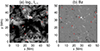 |
Fig. 1. Locations of the selected events. (a) Intensity map of the Si IV line integrated over 16 minutes. (b) Magnetogram averaged over 16 minutes, saturated at ±1000 G. The red crosses in (a) and (b) indicate the locations of the selected events. See Sect. 2. |
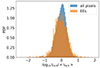 |
Fig. 2. Probability density function (PDF) of the Fe X line intensity for all pixels (in blue) and those identified as explosive events (in orange). ⟨IFe X⟩ represents the average intensity of the Fe X line across all pixels. See Sect. 2. |
3. Results
3.1. Overview of the three examples
In this section we present the synthesized transition region and narrowband coronal images, as well as the Si IV line profiles within the events analyzed in this study as an overview. The first example is shown in Fig. 3. This event exhibits a compact transient brightening in the Si IV intensity map. It also reveals faint emission enhancement in the EUI 174 Å passband. The blue box in Fig. 3a corresponds to one pixel in the Si IV line profile maps, with a pixel size of 240 km. The corresponding Si IV line profile shown in Fig. 3c clearly exhibits two peaks, one at the blue wing with a Doppler shift of ∼50 km s−1 and the other at the red wing with a shift of ∼20 km s−1. The two peaks of the line profile represent the bi-directional flows along the vertical direction within the blue box. We refer to this case as Event 1.
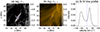 |
Fig. 3. Intensity maps and the Si IV line profile for Event 1. (a) Intensity map of the Si IV 1394 Å line. (b) Synthesized emission in EUI 174 Å passband. (c) Degraded Si IV line profile at the blue box shown in panels a and b. The size of the blue box is ∼240 km. The intensity is shown in arbitrary units. The vertical dashed blue line represents zero shift. See Sect. 3.1. |
The second example presented in Fig. 4 exhibits great emission enhancement in both the Si IV line and the EUI 174 Å image. This example was also identified as a transient coronal brightening analyzed in Chen et al. (2021, Fig. 3 therein), and here we present another snapshot that corresponds to the earliest time when the case is visible as a brightening in the synthesized EUI 174 Å images. The line profiles within the example shown in Fig. 4c strongly deviate from Gaussian. The profiles at the other snapshots also show wing enhancement, but it is not as obvious as that shown in Fig. 4c compared to the emission near the line center. There is one peak at the red wing with a Doppler shift of ∼35 km s−1, except for the peak near the rest wavelength, and the strong blue wing enhancement extends up to ∼70 km s−1. We reported that this event was generated by magnetic reconnection between two adjacent bundles of field lines in Chen et al. (2021). The reconnection outflows in and around the reconnection site are associated with the emission enhancement at the wings, and as a result the Si IV line exhibits a multi-peak broadened profile. We refer to this case as Event 2.
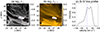
The third example presented in Fig. 5 also reveals enhanced emission in both the Si IV line and the EUI 174 Å passband. It is worth mentioning that the intensity enhancement in the 174 Å passband was not strong enough to be identified as a brightening in Chen et al. (2021). The Si IV line profile identified as an explosive events was 60 s before the snapshot shown in Fig. 5 at the same location, and the profile exhibits double peaks similar to the one shown in Fig. 3. In Fig. 5 we chose the time when the Si IV line and EUI 174 Å intensities were at maximum, and the Si IV profile was still non-Gaussian with red wing enhancement and strong line broadening. We refer to this case as Event 3. In this paper we focus on these three examples for a detailed case study. The overview of the other events is shown in Fig. A.1.
In addition, we obtained the spectral images of the Si IV line across the three events by using slits that were 50 Mm in length, positioned along the red dashed lines shown in Figs. 3–5. These spectral images are presented in Fig. 6. The three events exhibit clear wing enhancements that are distinct from other quiet-Sun regions, similar to the observations of explosive events described by Brueckner & Bartoe (1983). Furthermore, we present the temporal evolution of the Si IV line profiles at the locations of the three events in Fig. 7. The wing enhancements of these events were maintained for approximately two minutes, similarly to the findings reported by Dere et al. (1989).
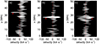 |
Fig. 6. Spectral images of the Si IV line. (a) Spectral image of the Si IV line across Event 1 along the red dashed line shown in Fig. 3a. The vertical dashed red line represents zero shift. The red arrow points to the location of Event 1. (b) Similar to (a), but for Event 2 shown in Fig. 4. (c) Similar to (a), but for Event 3 shown in Fig. 5. See Sect. 3.1. |
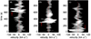 |
Fig. 7. Temporal evolution of the Si IV line profiles. (a) Temporal evolution of the Si IV line profile within the blue box at Event 1 shown in Fig. 3a. The vertical dashed red line represents zero shift. The red arrow points to the moment shown in Fig. 3. (b) Similar to (a), but for Event 2 shown in Fig. 4. (c) Similar to (a), but for Event 3 shown in Fig. 5. See Sect. 3.1. |
3.2. Evolution of magnetic field structure
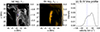
Since the plasma β is considerably less than one around all three events, they are dominated by changes in the magnetic field. To understand their generation mechanisms, we investigated the temporal evolution of the magnetic field structure in and around these events. For Event 1, we first selected 20 seed points in and around the region with enhanced Si IV intensity when the Si IV intensity reaches its peak. Then we traced the field lines from the seed points in both directions, as shown in Fig. 8a1. In order to follow the evolution of the magnetic field structure, we traced the field lines from the same seed points in different snapshots. We also present the field lines when the explosive event disappears (i.e., one minute after the Si IV intensity reaches its peak) in Fig. 8a2. We find that there are two bundles of magnetic field lines interacting in and around Event 1. When the event disappears, the magnetic field structure changes and only the field lines along the y-direction remain. In other words, the event is associated with magnetic reconnection between two bundles of field lines. The magnetic field structures during and after the occurrence of Event 2 are presented in Figs. 8b1 and b2, and these two panels are reproduced from Chen et al. (2021). There are two bundles of field lines forking when Event 2 occurs, and the event is located at the region where the two field line bundles diverge. After the event disappears, only the field line bundle along the x-direction remains. Thus, Events 1 and 2 are both triggered by the interaction between two field line bundles. It is worth mentioning that this magnetic field topology works for most coronal brightenings studied in Chen et al. (2021).
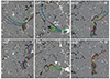 |
Fig. 8. Magnetic field structure evolution. (a1) Background showing a zoomed-in view of the vertical magnetic field in the photosphere. The magnetogram saturates at ±350 G. The curves represent the magnetic field lines passing through Event 1. The corresponding time is the same as in Fig. 3. (a2) Similar to (a1), but for the magnetogram and magnetic field lines one minute later. The white boxes indicate the location of the event. (b1) and (b2) Similar to (a1) and (a2), but for Event 2. The time difference of the two panels is 9 min. Reproduced from Chen et al. (2021). (c1) and (c2) Similar to (a1) and (a2), but for Event 3. The field of view for all panels represents a small part of the overall calculation domain. See Sect. 3.2. |
We also present the magnetic field structure in and around Event 3 in Fig. 8c1, and this event occurs in a highly twisted flux rope. When the Si IV brightening disappears, the field lines are highly relaxed, as shown in Fig. 8c2. It is possible that magnetic reconnection between field lines within the flux rope contributes to the relaxation of the flux rope and triggers the explosive event. The evolution of the magnetic field structure is similar to one case studied in Chen et al. (2021), where the coronal brightening is also associated with an untwisting flux rope. It is worth mentioning that the changes in the zoomed-in view of magnetograms are mainly the evolution of internetwork magnetic field patches, while the locations of the magnetic concentrations that form network patterns remain stable during the 16-minute period.
To summarize, the three events are all associated with changes in magnetic field topology. Events 1 and 2 are related to the interaction between two bundles of field lines, while Event 3 occurs in an untwisting flux rope, and the magnetic field environments for the explosive events are similar to the brightest coronal brightenings in the model. Thus, magnetic reconnection with small angles between field line bundles or within the twisted flux rope may trigger explosive events and/or coronal brightenings. However, some events are heated above 1 MK, while others barely reach typical coronal temperatures. Thus, it is necessary to understand why similar magnetic field topologies result in different thermal responses in different events.
3.3. Thermal responses
To examine the thermal properties of the three examples, we display the vertical cuts of various variables through the events. As shown in Fig. 9a, Event 1 is located between 2.5–4 Mm above the photosphere. The vertical velocity map shown in Fig. 9g clearly exhibits signatures of the bi-directional outflows, which correspond to the two peaks in the Si IV line profile shown in Fig. 3c. The decrease in the magnetic field strength and the enhancement of the heating rates (the sum of viscous and Joule heating) around the event (see Figs. 9h and i) imply that magnetic reconnection takes place, which is consistent with the magnetic field evolution shown in Fig. 8. The event also exhibits a little enhanced EUI 174 Å emission next to the Si IV brightening. Considering that EUI 174 Å emission has a contribution from both the Fe X 174 Å line (hot component) and the O VI 173 Å line (cool component), we also present the emission of the two lines in Figs. 9b and c. There is almost no Fe X emission within the event, but there is emission above, and the emission patterns of EUI 174 Å passband and the O VI line overlap significantly. The temperature within the regions with enhanced EUI 174 Å emission mostly reaches up to 105.8 K. Thus, this event is dominated by the cool component.
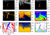 |
Fig. 9. Vertical cuts of (a) Si IV emission, (b) Fe X emission, (c) O VI emission, (d) EUI 174 Å emission, (e) temperature, (f) electron number density, (g) vertical velocity, (h) magnetic field strength, and (i) heating rates (sum of viscous and Joule heating) along the red dashed line through Event 1 shown in Fig. 3. The emissions are shown in arbitrary units. The contours outline the regions with enhanced Si IV emission. See Sect. 3.3. |
The vertical cuts for Event 2 are presented in Fig. 10. This event occurs at a height of 1.5–2 Mm, and the regions with enhanced Si IV emission are surrounding the EUI 174 Å brightening. The transition region and coronal emissions are mainly from the shell and core of the brightening, respectively. Similar to Event 1, there is a decrease in magnetic field strength within the event and the heating rates are enhanced around it, which are signatures of magnetic reconnection. The deviation from Gaussian of the Si IV line profile stems from the upflows and downflows around the reconnection site. The temperature of this event exceeds 2 MK, and the EUI 174 Å emission is dominated by the Fe X line. In other words, this event is dominated by the hot component. Compared to Event 1, the number density within the EUI 174 Å brightening is roughly the same (1010 cm−3). However, the magnetic field strength around Event 2 is ∼150 G, which is about one order of magnitude higher than that surrounding Event 1 (∼15 G). As a result, the heating rates are much higher in Event 2. Thus, the temperature difference between Events 1 and 2 results from the difference in the amount of converted magnetic energy.
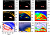 |
Fig. 10. Similar to Fig. 9, but along the red dashed line through Event 2 shown in Fig. 4. See Sect. 3.3. |
Figure 11 shows vertical cuts through Event 3. The vicinity of the reconnection region also reveals a decrease in magnetic field strength, an increase in heating rates, and clear bi-directional flow patterns. The height of this event in in the range 3–5 Mm, and the region with enhanced Si IV emission surrounds the EUI 174 Å brightening. Similarly to Event 2, the EUI 174 Å emission is dominated by Fe X and the O VI emission is mainly located at the edge of the coronal brightening. In this snapshot, the temperatures within the event reach above 1 MK. The surrounding magnetic field strength is ∼15 G, similar to that of Event 1. Moreover, the heating rates as well as the converted magnetic energy of Events 1 and 3 are comparable. Nevertheless, the density is 109.5 − 10 cm−3, which is much lower than that in Event 1. Thus, the temperature discrepancy is mainly due to the density difference in and around the reconnection region.
 |
Fig. 11. Similar to Fig. 9, but along the red dashed line through Event 3 shown in Fig. 5. See Sect. 3.3. |
4. Discussions
In this study we first investigated the magnetic field topology around the explosive events. Two events are located in the region where two bundles of field lines interact, and one example is associated with an untwisting flux rope. The magnetic field structures greatly change after the explosive events disappear, implying that the events are located at the reconnection region. The enhancement in current density and heating rates and the decrease in magnetic field strength in all the examples also indicate that magnetic reconnection occurs. Magnetic reconnection between the field line bundles or within the twisted flux rope triggers the bi-directional flow patterns, which result in the wing enhancement of the Si IV line profiles. Chen et al. (2021) investigated the magnetic field environment of the strongest coronal brightenings in the same model and found that the energetic coronal events are mostly triggered by component reconnection between the different field line bundles. A similar rearrangement of the tangled magnetic field and associated heating has also been found within cool transition region loops (Li et al. 2014), hot active region loops (Reale et al. 2019), and post-flare loops (Parenti et al. 2010). In addition, there is one example related to the relaxation of a highly twisted flux rope, which may explain the small-scale transient coronal brightenings accompanied by cool plasma structure (Panesar et al. 2021). In other words, different types of reconnection events (e.g., transient coronal brightenings and explosive events) in our self-consistent quiet-Sun model may share the common magnetic field environments (i.e., component reconnection).
The scenario of component reconnection, either between different field line bundles or within a flux rope, triggering the explosive events is different from magnetic field setups of most 2D reconnection models of explosive events, in which explosive events are often generated through anti-parallel reconnection (e.g., Roussev et al. 2001b; Innes et al. 2015; Peter et al. 2019). The magnetic field setups in the 2D models are inspired by the connection between explosive events and magnetic field changes in the photosphere (i.e., flux emergence and cancellation) (e.g., Chae et al. 1998; Muglach 2008). In a 3D model of an ephemeral emerging flux region with a higher level of photospheric magnetic field activities, Tiwari et al. (2022) found that some small-scale coronal brightenings are associated with magnetic reconnection between an emerging flux and an emerged–preexisting flux. However, the magnetic field in the photosphere is generated and maintained by the small-scale dynamo in our model, and hence our model represents the very quiet Sun without large-scale flux emergence or preexisting fields. The lower level of photospheric magnetic activities in our model might explain the reason that the selected explosive events and coronal brightenings in our model occur at coronal heights and are not directly related to the magnetic evolution in the photosphere. At least, our model can explain explosive events and coronal brightenings without signatures of magnetic field evolution in the photosphere (Muglach 2008; Panesar et al. 2021).
Although there are similar magnetic field environments, the temperatures of these events can be quite different. Events 2 and 3 are heated above 1 MK, while Event 1 barely reaches typical coronal temperatures. In principle, the temperature depends on density and the amount of converted energy, or heating rates. Compared to Event 1, the magnetic field strength, and hence heating rates, are higher in Event 2 and the density is comparable, while the density is much lower in Event 3 and the heating rates are similar. Thus, the peak temperature of reconnection events is constrained by both heating rates and density. Using a series of X-type neutral point reconnection models, Peter et al. (2019) suggested that the maximum temperatures in the vicinity of reconnection events and plasma β follow a power-law distribution. As a subsequent study, we will perform a statistical analysis of explosive events in our model to examine whether the relationship between peak temperatures and plasma β also follows a power-law distribution.
In order to quantitatively investigate the contribution of plasma, respectively with transition region and coronal temperatures, we artificially divided the EUI 174 Å emission into two parts, a cool and a hot component ( and
and  calculated in Sect. 2). The intensity variations of the EUI 174 Å passband and its two components of the three events are shown in Fig. 12. Event 1 barely reaches coronal temperatures, and the variation in the EUI 174 Å intensity is dominated by the cool component. The hot component is higher than the cool component, but the hot component is mainly from the coronal emission above the event (see Fig. 9) and exhibits as a background emission fluctuation. Events 2 and 3 are heated up to typical coronal temperatures, and their EUI 174 Å emissions are dominated by the hot component.
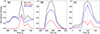 |
Fig. 12. Light curves of Event 1. (a) Intensity variations of EUI 174 Å passband in Event 1. The black solid curves represent the intensity variations of synthesized EUI 174 Å emission within the blue box shown in Fig. 3. The blue and red curves represent the cool and hot components, respectively. (b) and (c) Similar to (a), but for Events 2 and 3 shown in Figs. 4 and 5, respectively. For each panel, the three light curves are normalized by the maximum value of the black curve. The vertical black dashed lines represent the time of the snapshots shown in Figs. 3, 4, and 5, respectively. See Sect. 4. |
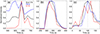 |
Fig. 13. Similar to Fig. 12, but for the intensity variations of the synthesized Fe VI (blue) and O VI (red) lines. The light curves of the EUI 174 Å passband are also presented as black solid lines. See Sect. 4. |
In addition, the intensity variations of the Fe X and O VI are shown in Fig. 13. We used the O VI 173 Å line because of its contribution to the EUI 174 Å passband. Explosive events can also be identified from the O VI 1032 Å line (e.g., Teriaca et al. 2004), and Huang et al. (2023) investigated spectral observations including the 1032 Å line of small-scale coronal brightenings taken by SPICE. We synthesized the intensity maps of the O VI 1032 Å line for several snapshots and compared them to the 173 Å line intensity maps. The intensity patterns of these two lines are almost the same, although the intensity ratio changes considerably because the formation temperatures of the two O VI lines are almost the same, while their line ratio is sensitive to the temperature. Moreover, the intensity variation of the 1032 Å line exhibits a similar tendency to the 173 Å line. Thus, we chose the 173 Å line for the following analyses. The light curves of the O VI and Fe X line roughly follow the cool and hot components of the EUI 174 Å passband shown in Fig. 12, respectively. For Event 1, the O VI line exhibits significant emission enhancement when the EUI 174 Å emission peaks, but the Fe X line does not because the intensity variation in this event is dominated by the cool component and the O VI line, and the Fe X emission is mainly from the coronal background above the event. For Event 2 the intensity variations in the Fe X and O VI lines are both similar to that of EUI 174 Å. At the first snapshot when Event 2 occurs, its temperatures are greater than 2 MK at the core and decrease to 104.5 K at the edge. Thus, the hot and cool components increase simultaneously at the beginning. During the magnetic reconnection process, the pressure near the reconnection sites is greatly enhanced, and the plasma therein expands. As a result, the density drops and the emissions from the different temperature ranges decrease together. The light curve of the Fe X line in Event 3 also follows the tendency of EUI 174 Å. Interestingly, the intensity variation in the O VI line in Event 3 shows double peaks, and the Fe X line reaches its peak between the separated peaks of the O VI line. It is consistent with one event investigated in Huang et al. (2023). They found that the light curve of the C III (formation temperature of 104.85 K) line also exhibits double peaks, and the O VI and Ne VIII lines reach their peaks in between. It was explained as the heating and cooling of the event. However, we examined the light curve of the Si IV line in Event 3, and it only shows one peak at t = 40 s. After examining vertical cuts for this event at different snapshots, we found that the average temperature within the EUI 174 Å brightening gradually increases from ≤104.0 K at t = 0 s to ∼106.0 K at t = 100 s, and slightly decreases at t = 120 s. Thus, the plasma heating and subsequent cooling can explain the Fe X intensity peak between the two peaks of the O VI line. Then the density quickly drops since t = 140 s due to the swift untwisting of the flux rope. It results in a rapid intensity decrease in the Fe X and the O VI lines because the emissivity is proportional to ne2. In other words, the intensity variations in Events 2 and 3 are first dominated by temperature changes and then density variations. Our analyses are based on examining the vertical cuts, and corks may need to be introduced into similar models to draw a more comprehensive and accurate picture of the temporal evolution of temperature and density and their responses in emissions (Druett et al. 2022).
It is straightforward to determine whether the events are heated to typical coronal temperatures from spectral observations of coronal emission lines, but it is very challenging to isolate the contribution of hot and cool components in coronal imaging observations. All AIA coronal channels have a contribution from the transition region lines (O’Dwyer et al. 2010; Del Zanna et al. 2011), and forward modeling with 3D MHD models indicates that the cool component cannot be neglected (Martínez-Sykora et al. 2011). Winebarger et al. (2013) suggested that some small-scale active region loops never reach 1 MK as their intensity in different AIA passbands peak at roughly the same time. Furthermore, Dolliou et al. (2023) performed a statistical time lag analysis with intensity variations of some transient small-scale coronal brightenings in EUI 174 Å and AIA coronal passbands. They found that the time lags are negligible and suggested that those events are dominated by cool components. To compare with their findings, we calculated the AIA emissions in different passbands and presented their light curves within the three events investigated in this study in Fig. 14. The intensity variations in the AIA passbands match very well for both Events 1 and 2, while Event 1 is dominated by the cool component and Event 2 is multi-thermal and dominated by the hot component. The cool and hot components of the EUI 174 Å emission show similar variations in Event 2; it is also valid for all AIA coronal passbands. The cadence of our model is 20 s, so it is also possible that the current temporal resolution of our model may not be sufficient to resolve the heating procedures, and hence the time lags between intensities in different passbands. The correlation among the light curves of the different passbands in Event 3 is weak. The peaks near t = 40 s in the 193 and 335 Å passbands are mainly contributed from the transition region lines with formation temperatures ≤105.5 K. The heating processes are more gentle than in Event 1, and the temperature gradually increases, resulting in various responses in different passbands. Thus, our analyses suggest that the co-temporal intensity variations in all AIA passbands have two possible explanations: the event is dominated by the cool component or it covers a wide temperature range with heating on short timescales.
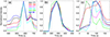 |
Fig. 14. Similar to Fig. 12, but for the light curves of the synthesized AIA images at different passbands. Each curve is normalized by its maximum value. See Sect. 4. |
5. Conclusions
In this study we isolated three explosive events in a 3D self-consistent MHD model of a quiet-Sun region. The Si IV line profiles within the events deviate strongly from Gaussian, indicating bi-directional flows triggered by magnetic reconnection. They appear along network lanes and last for approximately two minutes. Two events are located at the interacting regions of field line bundles, and one example is associated with a highly twisted flux rope. Their surrounding magnetic field structures are similar to those of the transient coronal brightenings studied in Chen et al. (2021). In addition, the magnetic field topologies greatly change after the events disappear, and the heating rates in and around the events are strong. Thus, explosive events in our model are manifestations of component reconnection.
Although explosive events may share similar magnetic field environments, their peak temperatures can be very different. The plasma within Event 1, like most events, barely reaches above 1 MK, while Events 2 and 3 both achieve typical coronal temperatures. By examining the vertical cuts of various parameters through the events, we found that temperature differences can result from a different amount of converted magnetic energy (i.e., heating rates) or local plasma density.
Furthermore, we investigated the light curves of AIA coronal passbands. Events 1 and 2 both exhibit simultaneous intensity variations in all AIA passbands, while they are dominated by the cool and hot components, respectively. Thus, the negligible time lags among AIA passbands cannot tell us whether the event is dominated by plasma at transition region temperatures. It is also possible that the heating processes are too fast to be resolved in observations. Moreover, the Fe X emission greatly increases within the events dominated by the hot component and exhibits background fluctuations within the event dominated by the cool component. Thus, spectral observations are necessary to determine the thermal properties, and future space missions such as Multi-slit Solar Explorer (MUSE; De Pontieu et al. 2022) and the EUV High-Throughput Spectroscopic Telescope (EUVST; Shimizu et al. 2019) are important to reveal their detailed thermal properties and heating processes.
Acknowledgments
We thank the anonymous referee for constructive comments. The work of Y.C. and D.P. was supported by the Deutsches Zentrum für Luft und Raumfahrt (DLR; German Aerospace Center) by grant DLR-FKZ 50OU2201. Y.C. acknowledges funding provided by the Alexander von Humboldt Foundation. We thank Dr. Luca Teriaca for helpful discussion. This research was supported by the International Space Science Institute (ISSI) in Bern, through ISSI International Team project #23-586 (Novel Insights Into Bursts, Bombs, and Brightenings in the Solar Atmosphere from Solar Orbiter).
References
- Antolin, P., Pagano, P., Testa, P., Petralia, A., & Reale, F. 2021, Nat. Astron., 5, 54 [NASA ADS] [CrossRef] [Google Scholar]
- Aschwanden, M. J., Tarbell, T. D., Nightingale, R. W., et al. 2000, ApJ, 535, 1047 [Google Scholar]
- Berghmans, D., Clette, F., & Moses, D. 1998, A&A, 336, 1039 [NASA ADS] [Google Scholar]
- Berghmans, D., Auchère, F., Long, D. M., et al. 2021, A&A, 656, L4 [NASA ADS] [CrossRef] [EDP Sciences] [Google Scholar]
- Bose, S., Henriques, V. M. J., Joshi, J., & Rouppe van der Voort, L. 2019, A&A, 631, L5 [NASA ADS] [CrossRef] [EDP Sciences] [Google Scholar]
- Brueckner, G. E., & Bartoe, J. D. F. 1983, ApJ, 272, 329 [Google Scholar]
- Chae, J., Wang, H., Lee, C.-Y., Goode, P. R., & Schühle, U. 1998, ApJ, 497, L109 [NASA ADS] [CrossRef] [Google Scholar]
- Chen, H., Zhang, J., Ma, S., Yan, X., & Xue, J. 2017, ApJ, 841, L13 [NASA ADS] [CrossRef] [Google Scholar]
- Chen, Y., Tian, H., Huang, Z., Peter, H., & Samanta, T. 2019, ApJ, 873, 79 [NASA ADS] [CrossRef] [Google Scholar]
- Chen, H., Zhang, J., De Pontieu, B., et al. 2020, ApJ, 899, 19 [Google Scholar]
- Chen, Y., Przybylski, D., Peter, H., et al. 2021, A&A, 656, L7 [NASA ADS] [CrossRef] [EDP Sciences] [Google Scholar]
- Chen, Y., Peter, H., Przybylski, D., Tian, H., & Zhang, J. 2022, A&A, 661, A94 [NASA ADS] [CrossRef] [EDP Sciences] [Google Scholar]
- Chitta, L. P., Peter, H., & Young, P. R. 2021, A&A, 647, A159 [NASA ADS] [CrossRef] [EDP Sciences] [Google Scholar]
- De Pontieu, B., Title, A. M., Lemen, J. R., et al. 2014, Sol. Phys., 289, 2733 [Google Scholar]
- De Pontieu, B., Testa, P., Martínez-Sykora, J., et al. 2022, ApJ, 926, 52 [NASA ADS] [CrossRef] [Google Scholar]
- Del Zanna, G., O’Dwyer, B., & Mason, H. E. 2011, A&A, 535, A46 [NASA ADS] [CrossRef] [EDP Sciences] [Google Scholar]
- Del Zanna, G., Dere, K. P., Young, P. R., & Landi, E. 2021, ApJ, 909, 38 [NASA ADS] [CrossRef] [Google Scholar]
- Dere, K. P. 1994, Adv. Space Res., 14, 13 [Google Scholar]
- Dere, K. P., Bartoe, J. D. F., & Brueckner, G. E. 1989, Sol. Phys., 123, 41 [Google Scholar]
- Dere, K. P., Bartoe, J. D. F., Brueckner, G. E., Ewing, J., & Lund, P. 1991, J. Geophys. Res., 96, 9399 [NASA ADS] [CrossRef] [Google Scholar]
- Dere, K. P., Landi, E., Mason, H. E., Monsignori Fossi, B. C., & Young, P. R. 1997, A&AS, 125, 149 [NASA ADS] [CrossRef] [EDP Sciences] [Google Scholar]
- Dolliou, A., Parenti, S., Auchère, F., et al. 2023, A&A, 671, A64 [NASA ADS] [CrossRef] [EDP Sciences] [Google Scholar]
- Dolliou, A., Parenti, S., & Bocchialini, K. 2024, A&A, 688, A77 [NASA ADS] [CrossRef] [EDP Sciences] [Google Scholar]
- Druett, M. K., Leenaarts, J., Carlsson, M., & Szydlarski, M. 2022, A&A, 665, A6 [NASA ADS] [CrossRef] [EDP Sciences] [Google Scholar]
- Handy, B. N., Acton, L. W., Kankelborg, C. C., et al. 1999, Sol. Phys., 187, 229 [Google Scholar]
- Hansteen, V. H., Archontis, V., Pereira, T. M. D., et al. 2017, ApJ, 839, 22 [NASA ADS] [CrossRef] [Google Scholar]
- Hansteen, V., Ortiz, A., Archontis, V., et al. 2019, A&A, 626, A33 [NASA ADS] [CrossRef] [EDP Sciences] [Google Scholar]
- Huang, Z., Teriaca, L., Aznar Cuadrado, R., et al. 2023, A&A, 673, A82 [NASA ADS] [CrossRef] [EDP Sciences] [Google Scholar]
- Innes, D. E. 2001, A&A, 378, 1067 [NASA ADS] [CrossRef] [EDP Sciences] [Google Scholar]
- Innes, D. E., & Tóth, G. 1999, Sol. Phys., 185, 127 [NASA ADS] [CrossRef] [Google Scholar]
- Innes, D. E., Brekke, P., Germerott, D., & Wilhelm, K. 1997a, Sol. Phys., 175, 341 [Google Scholar]
- Innes, D. E., Inhester, B., Axford, W. I., & Wilhelm, K. 1997b, Nature, 386, 811 [Google Scholar]
- Innes, D. E., Guo, L. J., Huang, Y. M., & Bhattacharjee, A. 2015, ApJ, 813, 86 [Google Scholar]
- Joshi, J., & Rouppe van der Voort, L. H. M. 2022, A&A, 664, A72 [NASA ADS] [CrossRef] [EDP Sciences] [Google Scholar]
- Kahil, F., Hirzberger, J., Solanki, S. K., et al. 2022, A&A, 660, A143 [NASA ADS] [CrossRef] [EDP Sciences] [Google Scholar]
- Lemen, J. R., Title, A. M., Akin, D. J., et al. 2012, Sol. Phys., 275, 17 [Google Scholar]
- Li, L. P., Peter, H., Chen, F., & Zhang, J. 2014, A&A, 570, A93 [NASA ADS] [CrossRef] [EDP Sciences] [Google Scholar]
- Lloyd, S. 1982, IEEE Trans. Inf. Theor., 28, 129 [CrossRef] [Google Scholar]
- Madjarska, M. S. 2019, Liv. Rev. Sol. Phys., 16, 2 [Google Scholar]
- Martínez-Sykora, J., De Pontieu, B., Testa, P., & Hansteen, V. 2011, ApJ, 743, 23 [Google Scholar]
- Muglach, K. 2008, ApJ, 687, 1398 [NASA ADS] [CrossRef] [Google Scholar]
- Müller, D., St. Cyr, O. C., Zouganelis, I., et al. 2020, A&A, 642, A1 [Google Scholar]
- Ni, L., Chen, Y., Peter, H., Tian, H., & Lin, J. 2021, A&A, 646, A88 [NASA ADS] [CrossRef] [EDP Sciences] [Google Scholar]
- O’Dwyer, B., Del Zanna, G., Mason, H. E., Weber, M. A., & Tripathi, D. 2010, A&A, 521, A21 [Google Scholar]
- Panesar, N. K., Tiwari, S. K., Berghmans, D., et al. 2021, ApJ, 921, L20 [CrossRef] [Google Scholar]
- Parenti, S., Reale, F., & Reeves, K. K. 2010, A&A, 517, A41 [NASA ADS] [CrossRef] [EDP Sciences] [Google Scholar]
- Peter, H., Huang, Y. M., Chitta, L. P., & Young, P. R. 2019, A&A, 628, A8 [NASA ADS] [CrossRef] [EDP Sciences] [Google Scholar]
- Purkhart, S., & Veronig, A. M. 2022, A&A, 661, A149 [NASA ADS] [CrossRef] [EDP Sciences] [Google Scholar]
- Reale, F., Testa, P., Petralia, A., & Graham, D. R. 2019, ApJ, 882, 7 [NASA ADS] [CrossRef] [Google Scholar]
- Rempel, M. 2017, ApJ, 834, 10 [Google Scholar]
- Rochus, P., Auchère, F., Berghmans, D., et al. 2020, A&A, 642, A8 [NASA ADS] [CrossRef] [EDP Sciences] [Google Scholar]
- Roussev, I., Doyle, J. G., Galsgaard, K., & Erdélyi, R. 2001a, A&A, 380, 719 [NASA ADS] [CrossRef] [EDP Sciences] [Google Scholar]
- Roussev, I., Galsgaard, K., Erdélyi, R., & Doyle, J. G. 2001b, A&A, 370, 298 [NASA ADS] [CrossRef] [EDP Sciences] [Google Scholar]
- Shimizu, T., Imada, S., Kawate, T., et al. 2019, SPIE Conf. Ser., 11118, 1111807 [NASA ADS] [Google Scholar]
- Skan, M., Danilovic, S., Leenaarts, J., Calvo, F., & Rempel, M. 2023, A&A, 672, A47 [NASA ADS] [CrossRef] [EDP Sciences] [Google Scholar]
- SPICE Consortium (Anderson, M., et al.) 2020, A&A, 642, A14 [NASA ADS] [CrossRef] [EDP Sciences] [Google Scholar]
- Teriaca, L., Madjarska, M. S., & Doyle, J. G. 2002, A&A, 392, 309 [NASA ADS] [CrossRef] [EDP Sciences] [Google Scholar]
- Teriaca, L., Banerjee, D., Falchi, A., Doyle, J. G., & Madjarska, M. S. 2004, A&A, 427, 1065 [NASA ADS] [CrossRef] [EDP Sciences] [Google Scholar]
- Tian, H., DeLuca, E. E., Cranmer, S. R., et al. 2014, Science, 346, 1255711 [Google Scholar]
- Tiwari, S. K., Hansteen, V. H., De Pontieu, B., Panesar, N. K., & Berghmans, D. 2022, ApJ, 929, 103 [NASA ADS] [CrossRef] [Google Scholar]
- Vögler, A., Shelyag, S., Schüssler, M., et al. 2005, A&A, 429, 335 [Google Scholar]
- Winebarger, A. R., Updike, A. C., & Reeves, K. K. 2002, ApJ, 570, L105 [NASA ADS] [CrossRef] [Google Scholar]
- Winebarger, A. R., Walsh, R. W., Moore, R., et al. 2013, ApJ, 771, 21 [NASA ADS] [CrossRef] [Google Scholar]
Appendix A: Additional examples of explosive events
In the main text, we presented detailed studies of three examples. Here we provide an overview of other randomly selected events in the same format as in Fig. 3.
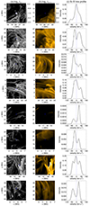 |
Fig. A.1. Intensity maps and the Si IV line profiles for the other events. Each row is analogous to Fig. 3, but for different events. See Appendix A. |
All Tables
All Figures
|
Fig. 1. Locations of the selected events. (a) Intensity map of the Si IV line integrated over 16 minutes. (b) Magnetogram averaged over 16 minutes, saturated at ±1000 G. The red crosses in (a) and (b) indicate the locations of the selected events. See Sect. 2. |
| In the text | |
|
Fig. 2. Probability density function (PDF) of the Fe X line intensity for all pixels (in blue) and those identified as explosive events (in orange). ⟨IFe X⟩ represents the average intensity of the Fe X line across all pixels. See Sect. 2. |
| In the text | |
|
Fig. 3. Intensity maps and the Si IV line profile for Event 1. (a) Intensity map of the Si IV 1394 Å line. (b) Synthesized emission in EUI 174 Å passband. (c) Degraded Si IV line profile at the blue box shown in panels a and b. The size of the blue box is ∼240 km. The intensity is shown in arbitrary units. The vertical dashed blue line represents zero shift. See Sect. 3.1. |
| In the text | |
|
Fig. 6. Spectral images of the Si IV line. (a) Spectral image of the Si IV line across Event 1 along the red dashed line shown in Fig. 3a. The vertical dashed red line represents zero shift. The red arrow points to the location of Event 1. (b) Similar to (a), but for Event 2 shown in Fig. 4. (c) Similar to (a), but for Event 3 shown in Fig. 5. See Sect. 3.1. |
| In the text | |
|
Fig. 7. Temporal evolution of the Si IV line profiles. (a) Temporal evolution of the Si IV line profile within the blue box at Event 1 shown in Fig. 3a. The vertical dashed red line represents zero shift. The red arrow points to the moment shown in Fig. 3. (b) Similar to (a), but for Event 2 shown in Fig. 4. (c) Similar to (a), but for Event 3 shown in Fig. 5. See Sect. 3.1. |
| In the text | |
|
Fig. 8. Magnetic field structure evolution. (a1) Background showing a zoomed-in view of the vertical magnetic field in the photosphere. The magnetogram saturates at ±350 G. The curves represent the magnetic field lines passing through Event 1. The corresponding time is the same as in Fig. 3. (a2) Similar to (a1), but for the magnetogram and magnetic field lines one minute later. The white boxes indicate the location of the event. (b1) and (b2) Similar to (a1) and (a2), but for Event 2. The time difference of the two panels is 9 min. Reproduced from Chen et al. (2021). (c1) and (c2) Similar to (a1) and (a2), but for Event 3. The field of view for all panels represents a small part of the overall calculation domain. See Sect. 3.2. |
| In the text | |
|
Fig. 9. Vertical cuts of (a) Si IV emission, (b) Fe X emission, (c) O VI emission, (d) EUI 174 Å emission, (e) temperature, (f) electron number density, (g) vertical velocity, (h) magnetic field strength, and (i) heating rates (sum of viscous and Joule heating) along the red dashed line through Event 1 shown in Fig. 3. The emissions are shown in arbitrary units. The contours outline the regions with enhanced Si IV emission. See Sect. 3.3. |
| In the text | |
|
Fig. 10. Similar to Fig. 9, but along the red dashed line through Event 2 shown in Fig. 4. See Sect. 3.3. |
| In the text | |
|
Fig. 11. Similar to Fig. 9, but along the red dashed line through Event 3 shown in Fig. 5. See Sect. 3.3. |
| In the text | |
|
Fig. 12. Light curves of Event 1. (a) Intensity variations of EUI 174 Å passband in Event 1. The black solid curves represent the intensity variations of synthesized EUI 174 Å emission within the blue box shown in Fig. 3. The blue and red curves represent the cool and hot components, respectively. (b) and (c) Similar to (a), but for Events 2 and 3 shown in Figs. 4 and 5, respectively. For each panel, the three light curves are normalized by the maximum value of the black curve. The vertical black dashed lines represent the time of the snapshots shown in Figs. 3, 4, and 5, respectively. See Sect. 4. |
| In the text | |
|
Fig. 13. Similar to Fig. 12, but for the intensity variations of the synthesized Fe VI (blue) and O VI (red) lines. The light curves of the EUI 174 Å passband are also presented as black solid lines. See Sect. 4. |
| In the text | |
|
Fig. 14. Similar to Fig. 12, but for the light curves of the synthesized AIA images at different passbands. Each curve is normalized by its maximum value. See Sect. 4. |
| In the text | |
|
Fig. A.1. Intensity maps and the Si IV line profiles for the other events. Each row is analogous to Fig. 3, but for different events. See Appendix A. |
| In the text | |
Current usage metrics show cumulative count of Article Views (full-text article views including HTML views, PDF and ePub downloads, according to the available data) and Abstracts Views on Vision4Press platform.
Data correspond to usage on the plateform after 2015. The current usage metrics is available 48-96 hours after online publication and is updated daily on week days.
Initial download of the metrics may take a while.