| Issue |
A&A
Volume 693, January 2025
|
|
|---|---|---|
| Article Number | A30 | |
| Number of page(s) | 17 | |
| Section | Astrophysical processes | |
| DOI | https://doi.org/10.1051/0004-6361/202449937 | |
| Published online | 23 December 2024 | |
Cosmic-ray induced sputtering of interstellar formaldehyde ices
1
Univ. Grenoble Alpes, CNRS, IPAG, 38000 Grenoble, France
2
Centre de Recherche sur les Ions, les Matériaux et la Photonique, CIMAP-CIRIL-GANIL, Normandie Université, ENSICAEN, UNICAEN, CEA, CNRS, 14000 Caen, France
⋆ Corresponding authors; aurore.bacmann@univ-grenoble-alpes.fr; mathilde.faure@univ-grenoble-alpes.fr
Received:
11
March
2024
Accepted:
3
July
2024
Context. In the cold and dense regions of the interstellar medium (ISM), for example in prestellar cores, gas-phase chemical abundances undergo a steep decrease due to the freeze-out of molecules onto the dust grain surfaces. While the depletion of many species would bring molecular abundances to undetected levels within short timescales, non-thermal desorption mechanisms such as UV photodesorption or cosmic-ray sputtering allows the return of a fraction of the ice mantle species back to the gas phase and prevents a complete freeze-out in the densest regions. In the last decade much effort has been devoted to understanding the microphysics of desorption and quantifying molecular desorption yields.
Aims. H2CO is a ubiquitous molecule in the ISM and in the gas phase of prestellar cores, and is likely present in ice mantles, but its main desorption mechanism is unknown. In this paper our aim is to quantify the desorption efficiency of H2CO upon cosmic-ray impact in order to determine whether cosmic-ray induced sputtering could account for the H2CO abundance observed in prestellar cores.
Methods. Using a heavy-ion beam as a cosmic-ray analogue at the Grand Accélérateur National d’Ions Lourds (GANIL) accelerator, we irradiated pure H2CO ice films at 10 K under high vacuum conditions and monitored the ice film evolution with infrared spectroscopy and the composition of the sputtered species in the gas phase using mass spectrometry. We derived both the effective and intact sputtering yield of pure H2CO ices. In addition, using IRAM millimetre observations, we also determined the H2CO gas-phase abundance in the prestellar core L1689B.
Results. We find that H2CO easily polymerises under heavy-ion irradiation in the ice, and is also radiolysed into CO and CO2. In the gas phase, the dominant sputtered species is CO and intact H2CO is only a minor species. We determine an intact sputtering yield for pure H2CO ices of 2.5 × 10³ molecules ion−1 for an electronic stopping power of Se ∼ 2830 eV (1015 molecules cm−2)−1. The corresponding cosmic-ray sputtering rate is ΓCRD = 1.5 × 10¹⁸ζ molecules cm−2 s−1, where ζ is the rate of cosmic-ray ionisation of molecular hydrogen in the ISM. In the frame of a simple steady-state chemical model of freeze-out and non-thermal desorption, we find that this experimental cosmic-ray sputtering rate is too low (by an order of magnitude) to account for the observed H2CO gas-phase abundance we derived in the prestellar core L1689B. We find however that this abundance can be reproduced if we assume that H2CO diluted in CO or CO2 ices co-desorbs at the same sputtering rate as pure CO or pure CO2 ices.
Key words: astrochemistry / molecular processes / methods: laboratory: solid state / ISM: abundances / cosmic rays
© The Authors 2024
 Open Access article, published by EDP Sciences, under the terms of the Creative Commons Attribution License (https://creativecommons.org/licenses/by/4.0), which permits unrestricted use, distribution, and reproduction in any medium, provided the original work is properly cited.
This article is published in open access under the Subscribe to Open model. Subscribe to A&A to support open access publication.
1. Introduction
The chemistry of prestellar cores is characterised by high amounts of molecular depletion due to the freeze-out of gas-phase molecules onto interstellar dust grains. At the high densities prevailing in prestellar cores, molecules from the gas phase collide and stick to the grains, building up an ice mantle. Millimetre wave observations of rotational transitions indeed show a molecular abundance decrease for most species towards the core centres (e.g. Willacy et al. 1998; Caselli et al. 1999; Bacmann et al. 2002) where the densities are highest. Additionally, infrared observations have established the presence of several species in the solid phase of the dense interstellar medium (Whittet et al. 1983; Boogert et al. 2015), the details of which are now being revealed by the James Webb Space Telescope (JWST; Yang et al. 2022; McClure et al. 2023; Rocha et al. 2024).
The accretion timescale for CO molecules at a temperature of 10 K, expressed in years, can be estimated as tCO = 5 × 10⁹/nH2 where nH2 is the molecular H2 density (Bergin & Tafalla 2007). At the densities prevailing in prestellar cores, around 105 − 106 cm−3, this timescale is much shorter than typical core lifetimes of around 106 years (Könyves et al. 2015). In the absence of any efficient mechanism returning frozen-out molecules back to the gas-phase, CO and other molecules should be absent from the gas phase, contrary to what is observed in these regions: within 106 years, for a density of 5 × 105 cm−3, the molecular abundance should drop by several dozen orders of magnitude, while observations show a much more moderate drop of a few orders of magnitude (Pagani et al. 2012). Therefore, desorption mechanisms allowing the frozen-out molecules to return to the gas phase have to be considered (Leger 1983).
At typical prestellar core temperatures, around 10 K, the available thermal energy is insufficient to enable molecular desorption, but several non-thermal mechanisms have been invoked to account for the observed molecular abundances in the gas phase: UV photodesorption, cosmic-ray sputtering, desorption by cosmic-ray induced UV photons (secondary UV radiation), IR photodesorption, or reactive desorption, in which the exothermicity of grain surface reactions contributes to the release of the reaction’s products in the gas phase. In the last decades, experimental studies have endeavoured to characterise the efficiency of the various desorption processes. Photodesorption rates have been measured under broadband UV irradiation for molecules such as CO, N2, CO2, and H2O by Öberg et al. (2007, 2009b,c) or Muñoz Caro et al. (2010). Further work using monochromatic synchrotron UV radiation provided insights into the mechanisms governing UV photodesorption (e.g. Fayolle et al. 2011; Bertin et al. 2012; Fayolle et al. 2013). These experiments coupled with quadrupole mass spectrometry to detect ejected gas-phase species have revealed that some molecules can be fragmented upon UV irradiation so that the photodesorption yield of the intact molecules may represent only a minor component of the total photodesorbed fragments, as is the case for CH3OH (methanol), HCOOH (formic acid), CH3OCHO (methyl formate) (Bertin et al. 2016, 2023) and H2CO (formaldehyde) (Féraud et al. 2019). As an illustration, the photodesorption yield measured by Bertin et al. (2016) for intact CH3OH is two orders of magnitude smaller than previously derived from experiments using solely infrared spectroscopy ice measurements (Öberg et al. 2009a), showing that it is therefore essential to monitor the products of the desorption process and not only the loss of the molecule in the solid state. Recent experiments of resonant infrared irradiation of CO and CH3OH ices suggest that IR photons could also induce desorption with a flux integrated efficiency similar to that of UV photons (Santos et al. 2023, and references therein).
Chemical desorption, or reactive desorption, occurs when the excess energy of a grain surface reaction (typically involving two radicals) can be converted into kinetic energy perpendicular to the surface overcoming the binding energy of the product with the grain (Allen & Robinson 1975). However, the efficiency of this process is difficult to evaluate in situ. Recent experiments have shown that while this mechanism can be efficient in some cases, the nature of the substrate (whether composed of bare graphite or covered with water ice) and its porosity (Dulieu et al. 2013), as well as the number of degrees of freedom of the reaction product plays a major role. In particular, Minissale et al. (2016) did not observe chemical desorption of CH3OH formed from the reaction CH3O + H, and estimated that the efficiency of chemical desorption from water ice is at most a few percent. Therefore, in the dense interstellar medium, where the composition of ice mantles is dominated by water ice, chemical desorption is expected to have a low efficiency, for large molecules at least.
Cosmic rays are also believed to contribute to molecular desorption (e.g. Leger et al. 1985; Willacy & Williams 1993; Hasegawa & Herbst 1993; Shen et al. 2004) by sputtering ice species to the gas phase. The cosmic-ray induced desorption process consists of two main contributions: the ‘whole-grain’ heating and the ‘thermal spike’ sputtering (erosion) (Bringa & Johnson 2004). While many studies so far have relied on the formalism proposed by Hasegawa & Herbst (1993) for whole-grain heating, cosmic-ray induced (thermal-spike) sputtering can be investigated experimentally by using swift heavy ions as cosmic-ray analogues. Studies of ice film irradiation by heavy ions carried out by Seperuelo Duarte et al. (2009, 2010) have determined sputtering yields for CO2 and CO ices by modelling the disappearance of the ice constituents from the solid phase. Of interest to account for the observed gas-phase abundances in the interstellar medium, however, is the amount of molecules that return to the solid phase intact per incident ion. Recent heavy-ion ice irradiation experiments coupled with a quadrupole mass spectrometer (QMS) to monitor the sputtered species in the gas phase (Dartois et al. 2019) have measured this parameter, both for pure ices (e.g. CO2, CH3OH, CH3OOCH3) and for ice mixtures (CH3OH/CO2, CH3OH/H2O, CH3OOCH3/H2O). For the species in these studies, a large fraction of the molecules are desorbed intact, and the sputtering yield of a minor species in an ice mixture is close to that of the species making up the bulk of the ice (Dartois et al. 2019).
While the above-mentioned experiments provide us with essential quantitative data regarding the desorption processes, they have been included in few chemical models so far, and it is still unclear whether they can account for observed molecular abundances (Wakelam et al. 2021). Moreover, a large body of experimental data is still missing, even regarding major species in the dense interstellar medium.
Formaldehyde (H2CO) is a ubiquitous species in molecular clouds and prestellar cores (e.g. Dieter 1973; Sandqvist & Bernes 1980; Mundy et al. 1987), with gas-phase column densities close to that of methanol, around 1013 − 1014 cm−2 in prestellar cores (Bacmann et al. 2003; Bacmann & Faure 2016) and in protostellar envelopes (Parise et al. 2006). In ice mantles, H2CO has only been tentatively detected towards protostellar envelopes and its abundance is estimated at around 5%, similar to CH3OH (Boogert et al. 2015; Rocha et al. 2024). Formaldehyde also represents an important intermediate step towards more complex molecules on grain surfaces (Chuang et al. 2016), or towards complex organic molecule precursors like HCO in the gas phase (Bacmann & Faure 2016). In prestellar cores, it is believed to form chiefly via hydrogenation of CO on grain surfaces (Watanabe et al. 2004; Minissale et al. 2016), as an intermediate step to methanol formation. Gas phase formation mechanisms have also been proposed (Guzmán et al. 2011; Ramal-Olmedo et al. 2021), but distinguishing both formation mechanisms requires detailed knowledge of the physical processes (e.g. desorption), which is lacking.
In this paper we present a study of swift ion irradiation of pure H2CO ices and determine the sputtering yield of the intact molecule. We calculate the sputtering rate over the cosmic-ray spectrum (from 100 eV/amu to 10 GeV/amu) and use it in a simple model to compare the derived H2CO gas-phase abundance with both H2CO observations in a prestellar source and the abundances predicted with other non-thermal desorption mechanisms.
The paper is organised as follows: In Sect. 2 we describe the irradiation experiments of thin H2CO films carried out at the Grand Accélérateur National d’Ions Lourds (GANIL, Caen, France) and in Sect. 3 the IRAM H2CO observations towards a prestellar core. In Sect. 4 we present the analysis of both the observational and the experimental data and determine the intact sputtering yield of the molecule. In Sect. 5 we discuss the astrophysical implications of our study and conclude in Sect. 6.
2. Experiments
Pure H2CO ice irradiation experiments were carried out at the GANIL ion accelerator on the IRRSUD beamline1 with the Irradiation de GLaces d’Intérêt AStrophysique (IGLIAS) setup (see Augé et al. 2018, for a detailed description) between May 14 and 16, 2021. The vacuum chamber was cryocooled down to a temperature of about 10 K, and held at a pressure of ∼5 × 10⁻¹⁰ mbar. Infrared spectra were collected with a Bruker Vertex 70v Fourier transform infrared spectrometer (FTIR), operating with a HgCdTe-detector and a 1 cm−1 spectral resolution. The angle between the spectrometer beam and the sample surface was 12°. Thin H2CO films with thicknesses of ∼0.53 μm were condensed on a ZnSe window at normal incidence with a needle placed at a distance of around 15 mm. The pressure during injection was typically 10−7 mbar. The deposition rate was adjusted to get a good optical quality, and the sample thickness was estimated using the band strengths of Bouilloud et al. (2015) and the interference fringes from the infrared spectra. Gas-phase H2CO was produced from the thermal decomposition of paraformaldehyde (Sigma Aldrich, purity 95%), heated at 100°C in a homemade oven maintained under secondary vacuum (∼10−7 mbar). The gaseous species sputtered in the chamber were detected with a MKS Microvision 2 QMS. The branching ratios of the species fragments were evaluated during their injection.
Irradiations were conducted with a 86Kr18+ beam of 0.86 MeV/u (74 MeV) corresponding to an electronic stopping power of 2830 eV (1015 molecules cm−2)−1 for an H2CO ice of 0.81 g cm−3 (Bouilloud et al. 2015), as computed with the SRIM-2013 code2 (Ziegler et al. 2010). The flux was 5 × 10⁸ ions cm−2 s−1, and the fluence reached at the end of the experiment was 4.36 × 10¹² ions cm−2. The corresponding doses are computed and compared to typical interstellar doses in Appendix A. Infrared spectra monitoring the ice composition were taken every two minutes starting from the beginning of the irradiation. The QMS continously scanned masses from 0–80 u, with a scan duration of ∼15 s.
Additionally, a control experiment under the same conditions was carried out in which we irradiated a ∼0.81 μm CO2 (Air Liquide, purity ≥99.998%) ice film with the same beam, corresponding to an electronic stopping power of 3290 eV (1015 molecules cm−2)−1, also computed with SRIM-2013, for a CO2 density of 1.0 g cm3 (Satorre et al. 2008). For this experiment, the flux varied between 1.1 × 10⁹ and 2.1 × 10⁹ ions cm−2 s−1 throughout the irradiation and the final fluence was 1013 ions cm−2.
3. Observations
Observations of one prestellar core, L1689B, were carried out between 2013 and 2019 during several campaigns, at the IRAM 30 m telescope, located at Pico Veleta, Spain. L1689B is situated in the Rho Ophiuchi star-forming region, and is characterised by low central temperatures and high central densities (Steinacker et al. 2016). It shows signs of gravitational contraction and appears dynamically evolved (Lee et al. 2001, 2003; Lee & Myers 2011) despite moderate molecular depletion and deuteration (Bacmann et al. 2003). A wealth of oxygen-bearing molecules, including formaldehyde and more complex organics, have been detected in this source (Bacmann et al. 2003, 2012). The observed coordinates are RA: 16h34m48.3s Dec:−24° 38′04″, corresponding to the peak of the millimetre continuum emission in the source. Several frequency setups were used to target rare isotopes of formaldehyde lines at 2 mm and 1 mm with the Eight MIxers Receivers (EMIR) E1 and E2, respectively. We focused on H2CO rotational transitions with upper energies typically lower than ∼40 K, as levels of higher energies are unlikely to be sufficiently populated at the low temperatures prevailing in the source (typically 10 K). Because the low-lying transitions of the main isotopologue are optically thick and self-absorbed towards the core centre (Bacmann et al. 2003), we present here observations of the optically thinner isotopologues H213CO and H2C18O, in both ortho and para nuclear-spin symmetries. The receivers were connected to the Fourier transform spectrometer (FTS) at a spectral resolution of ∼50 kHz over a bandwidth of 2 GHz, leading to velocity resolutions of ∼0.10 km s−1 at 2 mm and ∼0.07 km s−1 at 1 mm. The data were taken using the frequency switching procedure with a frequency throw of 7.5 MHz to reduce standing waves. Pointing and focus were typically checked every 1.5 − 2 h on nearby quasars or planets, with additional focus checks carried out shortly after sunset or sunrise. Pointing was found to be accurate to 3 − 4″. Calibrations were performed every 10 to 15 minutes, depending on atmospheric stability. The beam sizes vary from 18″ at 134 GHz to 11″ at 220 GHz. The beam efficiencies were taken following the Ruze formula  , with λ the wavelength, σ = 66 μm the surface rms of the 30 m antenna, and Beff, 0 = 0.863. The forward efficiencies were 93% and 91% at 2 mm and 1 mm, respectively. The spectra were converted from the antenna temperature scale Ta* to the main beam temperature scale Tmb using the values of the efficiencies given above.
The observational data were reduced with the Gildas/IRAM software3. The data reduction consisted in folding the spectra to recover the signal from the frequency switching procedure, except for the newer data for which folded spectra are delivered by the system. Then a low-order (typically 3) polynomial baseline was fitted to the spectra over line-less spectral regions and was subtracted before the spectra were co-added. The reduced spectra are presented in Appendix B. Finally, the spectral lines were fitted with Gaussians. The spectroscopic parameters of the observed transitions and results of the Gaussian fits are presented in Table1. The error given in the integrated intensity includes the calibration uncertainty, which was taken to be 15% at 2 mm and 20% at 1 mm.
Spectroscopic parameters of the observed lines.
4. Results
4.1. Experiments
The evolution of H2CO ice infrared (IR) spectra as a function of fluence is depicted in Fig. 1. At fluence zero, the film is made of pure H2CO, and neither paraformaldehyde nor CO or CO2 can be seen in the spectra. As soon as irradiation starts, bands characteristic of CO2 and CO appear, as well as bands around 2920, 1230, 1100, and 920 cm−1, which we attribute to the formation of an H2CO polymer (polyoxymethylene, hereafter POM). Conversely, H2CO bands decrease with fluence. Apart from CO, CO2, and POM, the infrared analysis shows no evidence of the formation of any other chemical species during the irradiation of H2CO. The column densities of CO2, CO, and H2CO were derived using the band strengths given in Table 2 and the integrated absorbance of the bands at 2343 cm−1, 2139 cm−1, and 1725 cm−1, respectively. The POM column density was calculated using a combination mode at 1105 cm−1 and a band strength of 1.9 × 10⁻¹⁸ cm molecules−1 (Noble et al. 2012). This band strength is not known with precision (Tadokoro et al. 1963; Schutte et al. 1993), and we assumed a factor of 2 uncertainty. An additional uncertainty arises from changes in the refractive index value across strong absorbance bands, resulting in some unphysical negative absorbances after baseline correction (see e.g. the C=O stretch of H2CO). The derived column density evolution as a function of fluence, with uncertainty zones, is presented in Fig. 2. As can be seen, the POM column density is not accurately determined, but it is consistent with a fast and efficient polymerisation of H2CO at very low fluence. Thus, at a fluence of 3 × 10¹¹ ions cm−1, the ice is mainly composed of POM.
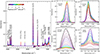 |
Fig. 1. IR spectra of irradiated H2CO ice. Left panel: Full range spectra, corrected for baseline, with assigned spectral peaks (see Table 2). Right panel: Focus on the evolution of the four bands used to derive column density of CO2, CO, H2CO, and POM in the ice. |
Peak position, assignments, and band strengths (at 25 K).
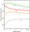 |
Fig. 2. Column density evolution of CO2, CO, H2CO, and POM ices as a function of fluence. In the case of POM, a factor of 2 uncertainty was assumed for the band strength of the combination mode at 1105 cm−1 (see text), as depicted by the shaded green zone. In the case of H2CO, the band strength of the stretching mode at 1725 cm−1 was also evaluated by Schutte et al. (1993) as 9.6×10⁻¹⁸ cm molecules−1 at 10 K, which corresponds to the highest column density value of the shaded red zone. Otherwise, an uncertainty of 20% was assumed for the band strengths. |
In similar experiments on non-polymerisable ices such as CH3OH and CO2 (Dartois et al. 2019; Seperuelo Duarte et al. 2009), the column density evolution with fluence can be solved through a simple differential equation involving solely radiolysis and sputtering processes (see e.g. Eq. (3) in Dartois et al. 2019). Here, however, we were not able to solve such a differential equation, due to the additional polymerisation process of H2CO towards POM, whose exact nature is unknown4. In addition, while swift ion irradiation of H2CO is responsible for the formation of POM, it also destroys POM to CO and CO2 (see the decrease in POM column density beyond a fluence of ∼3 × 10¹¹ ions cm−2 in Fig. 2). Therefore, in order to derive the sputtering yield, we resorted to another method based on the determination of the reduction in thin film thickness using the Fabry–Perot interference fringes observed in the infrared spectra (Dartois et al. 2020a, 2023), combined with QMS analysis of the gas composition. We emphasise that in order to validate this method, it was first applied to measure the thickness evolution of an irradiated thin film of CO2, for which the usual fit of the column density evolution via a differential equation was also possible. As reported in Appendix C, both methods were found to give consistent results, which are also in good agreement with the literature.
In the case of H2CO, as irradiation proceeds, the ice film becomes a mixture of mainly POM and H2CO for which the refractive index (n) is not available. Fitting the rigorous expression for the transmission (T) of a thin absorbing film on a thick transparent substrate is therefore not possible. Nevertheless, transmittance spectra follow a sinusoidal pattern, where the period is proportional to the thickness. Thus, we used the following simple expression to fit the transmittance spectra in the ranges of wavenumbers (1/λ) free of molecular absorptions:
Here T0 and A are free parameters, n is the refractive index taken as n = 1.33 ± 0.04 (Bouilloud et al. 2015), and d is ice thickness. The factor cos(12° ) corrects for the angle between the infrared beam and the sample. Fits obtained with this expression are shown in Fig. 3. The ice film is composed of POM and H2CO, with a composition changing during irradiation. Therefore, evaluating the sample mass density ρ is challenging. Furthermore, even the mass density of a pure H2CO ice film is unknown. Consequently, it is assumed to be constant at the value for liquid formaldehyde, ρ = 0.81 g cm−3 (Bouilloud et al. 2015), with an assumed uncertainty of 20%. It was used to derive the surface density of the ice σ = ρd, as a function of fluence, as shown in Fig. 4. The total mass sputtering yield can be directly estimated from the slope of the surface density evolution with fluence as Ym,tot = (1.8 ± 0.5) × 10−18 g ion−1. It should be noted that this total yield includes all sputtered species from the considered volume, both radiolysed species (C, O, H, H2, CO, and CO2) and intact H2CO fragments.
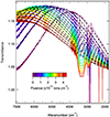 |
Fig. 3. Infrared transmittance spectra of a H2CO ice film evolution as a function of fluence. Solid lines: Experimental data. Dashed lines: Model spectra fitted to the data. See text for details. |
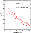 |
Fig. 4. Evolution of the surface density as a function of fluence deduced from interference fringes. The fit was performed for fluences greater than 6 × 10¹¹ ions cm−2 since the very beginning of the irradiation corresponds to ice compaction (e.g. Palumbo 2006; Dartois et al. 2013). |
In order to determine the chemical composition of the sputtered mass volume, the various fragments ejected into the gas phase were measured with the QMS. The small residual or background signal observed before irradiation was subtracted from the recorded signal during the whole irradiation time, as reported in Fig. 5 (top panel). We note that there is no intact sputtered POM as no signal is observed at m/z = 31, a mass characteristic of POM fragmentation pattern (Butscher et al. 2019; Duvernay et al. 2014). The mass m/z = 30 can be used to follow H2CO molecules since no fragment at this mass is observed in the CO fragmentation pattern (Fig. 6). Thus, the signals at m/z = 30 and m/z = 28 can be used to retrieve the total number of H2CO and CO species, respectively, by dividing each m/z signal by its relative contribution in the fragmentation pattern. The remaining signals at m/z = 12 and m/z = 16, after subtracting the contributions of CO and H2CO, indicate the abundances of C and O atoms, respectively. Once corrected for the total electron-impact ionisation cross-section σimpact(X) at 70 eV (energy of the QMS electron ionisation source), the relative fraction of each species f(X,g) with fluence F is determined (Fig. 5, bottom panel). QMS measurements at very low masses are not reliable, but the amount of hydrogen (H or H2) is supposed to be equal to the sum of the amounts of C, O, and CO. We note that CO2, a minor component of the ice (see Fig. 1), was not detected in the gas phase by the QMS. As irradiation proceeds, the composition of the film changes (Fig. 2) and this is also observed in the gas composition (Fig. 5, bottom panel). The fraction of gaseous H2CO thus decreases significantly (by approximately 70 %) for initial fluences (up to 2 × 10¹¹ ions cm−2), which is consistent with the radiolysis and the rapid polymerisation of solid H2CO. It then decreases more gradually, before a (noisy) slightly ascending plateau is reached beyond fluences of 3 × 10¹² ions cm−2. Conversely, the fractions of C and O increase rapidly (by approximately 70%), but also reach a plateau. Overall, the molecular fractions of these three chemical species in the gas vary by less than a factor of two. The larger molecular fractions of CO and H2 increase up to fluences of about 2 × 10¹² ions cm−2 before reaching a slightly descending plateau, with variations of less than 15%. We can extract the initial fraction of each species X in the gas phase fi(X,g) (Table 5), and the subsequent evolution f(X,g) was fitted by third-order polynomials.
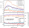 |
Fig. 5. QMS signals as a function of fluence. Top panel: Background corrected signals. Bottom panel: Molecular fractions in the gas (solid lines, left y-axis) derived from the fragmentation patterns and ionisation cross sections, and sputtering yield of each species (dashed lines, right y-axis). See text for details. |
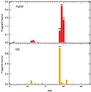 |
Fig. 6. Mass fragmentation pattern monitored during species injection (for ice sample deposition) for H2CO (top panel) and CO (unpublished data) (bottom panel). |
By combining the total mass sputtering yield Ym,tot with the fitted molecular fractions f(X,g), we can derive the sputtering yield of each ejected species YX(F),
where NA is the Avogadro constant, M(X) is the molecular mass of species X, and fm(X,g) represents the mass fraction of species X in the gas:
The derived sputtering yields for the various ejected species X are plotted as dashed lines in the bottom panel of Fig. 5 (right y-axis). Similarly to the molecular fractions, the intact sputtering yields vary by less than a factor of 2 for C, O, and H2CO, and by less than 15% for CO and H2, as expected. The average intact sputtering yields YX were computed over the full range of fluences and are listed in Table 5. The average sputtering yield for intact H2CO is found to be Yintact = YH2CO = (2.5 ± 2.3)×103 molecules ion−1.
We can now try to estimate the effective sputtering yield, Yeff. For non-polymerisable species, Yeff is usually determined using the column density evolution with fluence measured from IR spectroscopy (Dartois et al. 2019; Seperuelo Duarte et al. 2009). For a pure ice X, Yeff is defined as the semi-infinite thickness effective-sputtering yield for the ice under study. It includes both intact sputtered species X and radiolysed (daughter) sputtered species. Since radiolysis and sputtering occur simultaneously, IR spectroscopy captures the disappearance of H2CO, regardless of whether it is sputtered intact or radiolysed. Yeff is simply related to Yintact as

where η is the intact fraction of sputtered H2CO. In our experiment, the volume to be sputtered just before irradiation is composed of pristine H2CO ice. The impact of a swift heavy ion induces radiolysis along its track, affecting a fraction of this volume. Therefore, after irradiation has started, the sputtered volume is composed of intact H2CO, fresh products of radiolysis as well as primary radiolytic products that accumulate in the film (see Fig. 7). Therefore, in order to determine the effective sputtering yield Yeff, the intact fraction (η) of sputtered H2CO during irradiation must be estimated using the initial fractions reported in Table 3:
Total electron-impact ionisation cross-sections σimpact(X); initial fractions fi(X, g) and averaged sputtering yield YX.
 |
Fig. 7. Schematic timeline of events during the first impact of a swift heavy ion (SHI) on an ice sample, within the thermal spike model. Chemistry and sputtering occur almost simultaneously within 10−9 s of the ion’s passage (Lang et al. 2020). The length ds corresponds to the sputtering depth probed by an individual ion incident, which is inferior to d0, the initial ice film thickness; rr corresponds to the radiolysis destruction radius, which is at most equal to the sputtering cylinder radius rs (Dartois et al. 2021). Considering the timescales involved, infrared spectroscopy cannot observe the radiolysis effects within the sputtered volume during the passage of an ion. |
In practice, we derived an intact fraction of sputtered H2CO molecules η = 0.23 ± 0.03, corresponding to an effective sputtering yield for the H2CO film of Yeff = (10.9 ± 9.9)×103 molecules ions−1.
In their compendium of selected literature sputtering yields, Dartois et al. (2023) show that the sputtering yield induced by swift heavy ions follows an empirical law that is directly proportional to the square of the electronic stopping power Se:

Here, using a stopping power of 2830 eV (1015 molecules cm−2)−1 for the 86Kr18+ beam, we obtain for a pure H2CO ice Y0 = (3.1 ± 2.8)×10−4 1030 eV−2 cm−4 molecule3. However, most studies only have access to the effective sputtering yield Yeff, which is therefore used for Yintact in Eq. (6) (e.g. Dartois et al. 2023). In this case, the effective prefactor value is Y0eff = (1.4 ± 1.3)×10−3 1030 eV−2 cm−4 molecule3.
4.2. H2CO abundance in L1689B
The H2CO column density in the L1689B prestellar core was determined using the RADEX radiative transfer code (van der Tak et al. 2007) in the uniform sphere approximation. The collisional rate coefficients used in the computation are the H2CO−H2 coefficients from Wiesenfeld & Faure (2013) adapted to the spectroscopy of H2C18O and H213CO and were obtained from the Excitation of Molecules and Atoms for Astrophysics (EMAA) collisional rate database5. Because there are no radiative or collisional mechanisms converting one form into the other, the ortho and para nuclear-spin isomers of each isotopologue were treated as two separate species. At thermal equilibrium, the ortho-to-para ratio of H2CO is ∼1.5 at 10 K, and reaches the statistical value of 3.0 at about 30 K. Only collisions with para-H2 were considered as the ortho-H2 abundance represents at most 1 − 10% of the total H2 (Pagani et al. 2009; Troscompt et al. 2009; Dislaire et al. 2012) and can be neglected in prestellar cores.
Using RADEX, we calculated grids of models for ranges of values in kinetic temperature, H2 density, and in the molecular column densities (ortho-H213CO, para-H213CO, ortho-H2C18O, or para-H2C18O). The grid points in temperature and H2 density were chosen to be the same for all species, which is based on the assumption that all of them are coexistent. The densities span a range between 5 × 104 cm−2 and 5 × 105 cm−2 and the temperatures between 3 K and 12 K. The column density of ortho-H213CO No13 was varied between 5 × 1011 cm−2 and 5 × 1012 cm−2. The column density of para-H213CO Np13 was taken as Np13 = No13/opr where opr is the ortho-to-para ratio in the considered H2CO isotopologue (either in H213CO or in H2C18O), and the free parameter opr was varied between 1 and 6. For the column density of H2C18O, we assumed a ratio cor = 13C/18O such as the ortho-H2C18O column density No18 is No18 = No13/cor and the para-H2C18O column density No18 is Np18 = No13/(cor × opr), and varied this ratio between 7 and 10 (see e.g. Wilson 1999, for standard values of 13C/18O). The input linewidths for the calculations were taken to be 0.48 km s−1 for H213CO and 0.38 km s−1 for H2C18O, but they have little influence on the results, because our fitting procedure relies on the velocity integrated intensities of the modelled lines compared to that of the observations. The goodness of fit was estimated with a χ2 defined as
where T is the kinetic temperature; n(H2) is the H2 density; Wobs is the observed line integrated intensity; σ is the error on the observed integrated intensity; Wmod is the line integrated intensity calculated by RADEX; and the indices i, j, k, l refer to the transitions in ortho-H213CO, para-H213CO, ortho-H2C18O, and para-H2C18O, respectively. Typically, 10 to 15 points were chosen for each parameter. The grids were refined close to parameter values best reproducing the observations. The best fitting parameters are given in Table 4.
Non-LTE model parameters best fitting the observed spectra.
Because the ortho-to-para ratio is expected to be at most 3 for H2CO6, we re-ran the model and kept the ortho-to-para ratio set to 3. In this case, the χ2 value is slightly worse (5.5 instead of 4.3 for the best model), and the best fitting temperature is slightly lower (closer to 9 K). The other parameters (density, ortho-H213CO column density, and 13C/18O ratio) remain unchanged. We also ran the fitting routine with the temperature and density values found for CH3OH by Bacmann & Faure (2016) (i.e. T = 8.5 K and nH2 = 3.6 × 105 cm−3), and again found results for the parameters very similar to the best fit: No13 = 1.8 × 1012 cm−2.
The line integrated intensities from the best fit model are shown in Fig. 8 against the observed line integrated intensities. The model can account for the observations within the uncertainties.
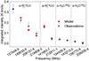 |
Fig. 8. Comparison between the observed integrated intensities (blue dots) and the integrated intensities derived from the non-LTE model (red diamonds), for each of the observed lines, labelled by their rest frequencies. In the figure, ‘o’ stands for ortho and ‘p’ stands for para. |
With the values in Table 4, we obtain the following values for the molecular column densities: No13 = 2.04 × 1012 cm−2, Np13 = 5.4 × 1011 cm−2, No18 = 2.2 × 1011 cm−2, and Np18 = 6 × 1010 cm−2. Assuming a ratio 16O/18O of 557 (Wilson 1999), we obtain a total (ortho + para) column density of 1.6 × 1014 cm−2 for the main isotopologue H2CO.
The H2 column density at the same position as the H2CO observations was derived from the model of Steinacker et al. (2016), by integrating the density profile along the line of sight and multiplying by two to account for the contribution of the far side of the core. The uncertainty was determined using the error bars from the fit including the interstellar radiation field (see Steinacker et al. 2016, for details). We find a total H2 column density NH2 = 1.3 × 1023 cm−2, with a spread 5 × 10²² − 2.1 × 1023 cm−2. The corresponding relative abundance of H2CO with respect to total hydrogen (nH = n(H)+2n(H2)) is ∼6 ± 4 × 10⁻¹⁰.
5. Astrophysical applications
5.1. Model
We investigate in this section whether non-thermal desorption from icy grains can explain the gas-phase abundance of H2CO derived in L1689B. A simple analytical model is employed: H2CO molecules from the gas phase can only accrete on the icy surface of dust grains, while H2CO molecules from the grain surface can only desorb via photodesorption (due to both external and internal cosmic-ray induced UV photons) and direct cosmic-ray induced sputtering.
In addition, a steady-state is assumed, with constant kinetic temperature, density, and total H2CO abundance (gas and ice) throughout the core. This total H2CO abundance is unknown in L1689B and taken as 3 × 10⁻⁶, which is the typical H2CO ice abundance in low-mass young stellar objects (LYSOS) (Boogert et al. 2015), corresponding to about 6% with respect to H2O ice7. The kinetic temperature T is fixed at 10 K and the H2 density at n(H2) = 2 × 105 cm−3, as reported in Table 4 for the L1689B core.
At steady-state, the rates of accretion and desorption are equal and we can write:
where nfg and nfs are the formaldehyde densities (in cm−3) in the gas and solid ice phase, respectively. The accretion rate (in s−1) can be written as

where ⟨πag2⟩ is the average grain surface (in cm2), ng the grain number density (cm−3), vth the thermal velocity of H2CO molecules, and S the sticking coefficient taken as 1.0. The desorption rate (in s−1) can be written as (Flower et al. 2005)
where ∑inis is the sum of ice abundances such that nfs/∑inis is the fractional abundance of H2CO in the ice. In the following, we note that ∑inis = XicesnH. The quantity Γtot is the total desorption rate (in molecules cm−2s−1) defined as

where ΓISRF, ΓCRI − UV, and ΓCRD are the desorption rates due to external UV photodesorption, cosmic-ray induced UV phodesorption, and direct cosmic-ray sputtering, respectively. We note that cosmic-ray induced whole-grain heating can be neglected for a thick volatile mantle, as found at high density (nH ≳ 104 cm−3) (Bringa & Johnson 2004; Wakelam et al. 2021).
5.2. Desorption rates
The external UV photodesorption rate can be written as

where IISRF is the external interstellar far-UV radiation field (averaged between 6 and 13.6 eV) of ∼108 photons cm−2 s−1 (Habing 1968); Av is the visual extinction; γ is a measure of UV extinction relative to visual extinction, which is about 2 for interstellar grains (Roberge et al. 1991); and Ypd is the photodesorption yield of H2CO (in molecules photon−1). The last value was recently determined in the laboratory by Féraud et al. (2019), who were able to derive an intact H2CO photodesorption yield of 4 − 10 × 10−4 molecule/photon in various astrophysical environments, including interstellar clouds and prestellar cores (see their Table 1). In the following we use an average experimental yield of Ypd = 7 × 10⁻⁴ molecule/photon for the photodesorption of intact H2CO.
The cosmic-ray induced UV photodesorption rate can be written as

where ICRI is now the internal UV field induced by the cosmic-ray excitation of H2, which was taken as ICRI ∼ 103ζ17, where ζ17 is the rate of cosmic-ray ionisation of molecular hydrogen ζ in units of 10−17 s−1 (see the definition of ζ below). This simple relation between ICRI and ζ17 was deduced from Fig. 4 of Shen et al. (2004), with ζ computed using Eqs. (16)–(17) below.
Finally, the direct cosmic-ray sputtering rate ΓCRD is computed by summing and integrating the product of the sputtering yield Ys(ϵ, Z) with the differential cosmic-ray flux j(ϵ, Z):
Here ϵ is the kinetic energy per nucleon, Z is the atomic number of the cosmic-ray nuclei, and Ys(ϵ, Z) is the sputtering yield in H2CO/ion obtained by combining the experimental yield Yintact(Se) for intact sputtering with the calculated electronic stopping power Se(ϵ, Z). It is multiplied by a factor of 2 to account for the entrance and exit points of the cosmic-rays through the grain. Assuming a quadratic dependence of Yintact(Se) with the stopping power, as in Eq. (6), the intact sputtering yield of H2CO molecules can be described as

where we combined Yintact = 2.5 × 10³ molecules ion−1 (see Table 3) with the stopping power of 2830 eV (1015 molecules cm−2)−1 for the 86Kr18+ beam.
In order to compute Ys(ϵ, Z) for a range of kinetic energies (see below), the SRIM-2013 code was used to compute the electronic stopping powers Se for an H2CO ice density of 0.81 g cm−3 and for the cosmic elements with the largest contributions, accounting for the ∼Z4 scaling of the sputtering yields (Dartois et al. 2023). In practice, the 15 ions of H, He, C, O, Ne, Mg, Si, S, Ca, Ti, V, Cr, Mn, Fe, and Ni were included using the fractional abundances f(Z) of Kalvāns (2016, their Table 1). It should be noted that iron, despite its low fractional abundance, gives the largest contribution (∼44%) to the rate, as already found by Seperuelo Duarte et al. (2010) for CO ice.
For the differential cosmic-ray flux j(ϵ, Z) (in particles cm−2 s−1 sr−1 (MeV/amu)−1) we adopted the functional form proposed by Webber & Yushak (1983)
where C(Z) = 9.42 × 10⁴f(Z) is a normalising constant and E0 a form parameter that varies between 0 and 940 MeV. This formulation corresponds to a primary spectrum since it neglects the energy-loss of cosmic rays through the dense interstellar gas. It allows, however, the full range of measured ionisation rates to be explored, from standard diffuse clouds (a few 10−16 s−1) to dense clouds (a few 10−17 s−1), by simply varying the parameter E0. In order to infer the relation between ΓCRD and ζ, the ionisation rate ζ was computed as in Faure et al. (2019, their Appendix A):
Here  is the cross-section for ionisation of H2 by proton impact, Φ is a correction factor accounting for the contribution of secondary electrons to ionisation, and where
is the correction factor for heavy nuclei ionisation. Full details and references can be found in Appendix A of Faure et al. (2019). In practice, the E0 parameter in Eq. (16) was taken in the range 200−900 MeV so that ζ was explored in the range 8 × 10⁻¹⁸ − 4 × 10⁻¹⁶ s−1. The integrals in Eqs. (14) and (17) were evaluated numerically from ϵmin = 100 eV/amu to ϵmax = 10 GeV/amu. The calibration plot between the intact sputtering rate of H2CO and the ionisation rate is displayed in Fig. 9 (black curve), where ΓCRD is found to scale linearly with the ionisation rate. We note that although the low-energy content (< 100 MeV) of the cosmic-ray spectrum is poorly constrained, the relation between ΓCRD and ζ was found to be quite robust.
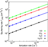 |
Fig. 9. Intact sputtering rate of pure H2CO and effective sputtering rates of the pure ices CO, CO2, and H2O as a function of the ζ cosmic-ray ionisation rate. Effective sputtering yield pre-factors are taken from Dartois et al. (2023). |
It is now interesting to compare the sputtering rate of H2CO with those of the main ice components of interstellar grains, that is H2O, CO, and CO2, where the latter two have a typical abundance of 20–30% with respect to H2O. Trace ice species such as NH3, CH4, H2CO, and CH3OH are expected to be embedded in H2O-rich, CO-rich, or CO2-rich layers. We assume that the intact sputtering yield of the trapped molecule is equal to the effective sputtering yield of the ice matrix. Simplistic but intuitive, this hypothesis is actually supported by irradiation experiments performed on methanol diluted in H2O and CO2 ice matrices, although the intact sputtering efficiency depends on the dilution factor8 (see the detailed discussions in Dartois et al. 2019, 2020b). We note that the effective sputtering yield of either water or CO2 was similarly employed to model the cosmic-ray induced sputtering of CH3OH in cold molecular cores (Wakelam et al. 2021; Paulive et al. 2022). The above procedure was thus applied to pure CO, CO2, and H2O ices using the effective sputtering yield pre-factors reported in Table 1 of Dartois et al. (2023) with ice densities (needed to compute Se) of 0.88 g cm−3, 1.0 g cm−3, and 0.94 g cm−3, respectively (Luna et al. 2022; Satorre et al. 2008; Bouilloud et al. 2015). The corresponding sputtering rates as functions of ζ are shown in Fig. 9. As expected, our results for CO, CO2, and H2O are in very good agreement with those of Dartois et al. (2023, see their Fig. 5). We can also observe that the intact sputtering rate of pure H2CO is a factor of 10–100 lower than the effective sputtering rates of H2O, CO, and CO2. For convenient use in astrochemical models, simple linear fits of the sputtering rates shown in Fig. 9 were performed over the range ζ = [8 × 10⁻¹⁸ − 10−16] s−1. These fits are reported in Table 5.
5.3. H2CO gas-phase abundance
Because the total abundance of formaldehyde ngtot is conserved, we have
By combining Eqs. (8–10) and (19), we obtain
Since in practice vthXicesnH/Γtot ≫ 1 and substituting  , where μ is the mass of H2CO, the H2CO gas-phase fractional abundance, Xfg = nfg/nH, takes the simple form
where Xftot = nftot/nH is the H2CO total fractional abundance, taken as 3 × 10⁻⁶ (see above). The total fractional abundance of ices, Xices, is unknown in L1689B, but again we can assume typical ice abundances in LYSOS, as compiled by Boogert et al. (2015, their Table 2). By including ‘securely’, ‘likely’, and ‘possibly’ identified species, we obtain Xices ∼ 8 × 10⁻⁵. Finally, using the physical conditions derived from H2CO emission in L1689B (i.e. T = 10 K and nH = 4 × 105 cm−3), we obtain numerically:
In order to reproduce the measured abundance in L1689B (∼6 × 10⁻¹⁰), a total desorption rate Γtot ∼ 50 molecules cm−2s−1 is required. We compare in Fig. 10 the observational abundance to our predictions from the above analytical model, assuming the cosmic-ray ionisation rate is ζ = 3 × 10⁻¹⁷ s−1 (i.e. ζ17 = 3), which is the typical ionisation rate in molecular clouds, where Av > 10 (see Fig. 19 in Indriolo & McCall 2012). Five different models are presented: desorption is either due to external and internal photons only (in orange) or to both photons and direct cosmic-ray sputtering, assuming H2CO ices are pure (in black) or embedded in H2O-rich (in blue), CO2-rich (in red), or CO-rich (in green) matrices. We can observe that photodesorption alone cannot explain the gas phase abundance of H2CO in L1689B and that direct cosmic-ray sputtering is much more efficient, except in the case of a pure H2CO ice. In particular, cosmic-ray sputtering of H2CO from CO-rich or CO2-rich ices can reproduce the gas phase abundance measured towards L1689B to within a factor of 3. Interestingly, this result is consistent with observational evidence that catastrophic CO freeze-out occurs at Av ≥ 9 and nH > 105 cm−3, where CO hydrogenation may form a CH3OH-rich layer including H2CO and new CO2 molecules (Boogert et al. 2015). It is also possible that part of the interstellar H2CO forms in the gas phase, for example via the barrierless reaction CH3 + O (see e.g. Terwisscha van Scheltinga et al. 2021). Thus, while the present results emphasise the potential role of direct cosmic-ray sputtering of H2CO molecules from CO-rich or CO2-rich ices, the importance of gas-phase formation and destruction of H2CO will need to be explored in future works. Finally, we note that the H2CO gas-phase abundance in L1689B corresponds to about 0.02% of the total (gas and ice) H2CO abundance.
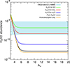 |
Fig. 10. H2CO gas phase abundance with respect to H nuclei as a function of visual extinction. The observational value derived in this study for the prestellar core L1689B (blue hatched zone) is compared to five different models for H2CO sputtering: pure H2CO ice and H2CO ideally diluted in H2O, CO2, and CO matrices. See text for details. |
In summary, our simple model shows that the yields for experimentally determined direct cosmic-ray sputtering are large enough to release significant amounts of H2CO ice into the gas-phase, provided that H2CO is embedded in CO-rich or CO2-rich ice mantles and that H2CO molecules co-desorb with the matrix (i.e. with the same yield). Obviously, further experiments with mixed ices (e.g. H2CO:CO), as well as more comprehensive (time-dependent and density-dependent) astrochemical models are needed to confirm these results.
6. Conclusions
We have studied the sputtering of pure formaldehyde ices under cosmic rays using swift-ion irradiation experiments of H2CO ice films at 10 K carried out at GANIL with the IGLIAS setup. Formaldehyde is found to quickly polymerise upon swift ion exposure. Other detected radiolysis products in the ice are CO and CO2. We determined the intact H2CO sputtering yield in the gas phase to be Yintact = 2.5 × 10³ molecule ion−1 for a stopping power of 2830 eV/1015 molecule cm−2. Assuming a quadratic dependence of the sputtering yield with stopping power, this corresponds to an intact sputtering prefactor Y0 = 3.1 × 10⁻⁴ 1030 eV−2cm−4molecule3. The effective sputtering prefactor is Y0eff = 1.4 × 10⁻³ 1030 eV−2cm−4molecule3. With these values we determined that the direct cosmic-ray sputtering rate for intact H2CO in pure ices can be expressed simply by ΓCRD(H2CO) = 0.15 ζ17 molecules cm−2 s−1, where ζ17 is the cosmic-ray ionisation rate in units of 10−17 s−1.
Using a simple steady-state chemical model including accretion of molecules from the gas phase onto the grains and their desorption by either UV photons (both external and secondary UV photons produced by cosmic-ray excitation of H2) or direct cosmic-ray impact, we find that photodesorption is not efficient enough to account for the gas-phase abundance of H2CO of 6 × 10⁻¹⁰ (with respect to H nuclei) measured in the prestellar core L1689B, nor is cosmic-ray induced sputtering of a pure H2CO ice. On the other hand, when H2CO is diluted in CO or in CO2 ices, our model can reproduce the H2CO gas-phase abundance, assuming that minor ice constituents like formaldehyde will be sputtered to the gas phase at the same effective rate as the ice mantle bulk. However, the cosmic-ray sputtering rate is insufficient if H2CO is embedded in a water ice mantle. Future experimental studies should be dedicated to investigating the polymerisation and sputtering of H2CO diluted in other ice matrices (e.g. H2O, CO, CO2). The competition between the cosmic-ray induced sputtering and the gas-phase chemistry of H2CO will also need to be explored.
Data availability
The experimental data can be downloaded from https://zenodo.org/records/13383307
A recent laboratory experiment has shown that the measured ortho-to-para ratio of H2CO molecules formed via UV photolysis of CH3OH ices is ∼3, with no correlation with ice temperature (Yocum et al. 2023).
This value is similar to the 4.1% recently measured by JWST towards the young-mass protostar NGC 1333 IRAS 2 (Rocha et al. 2024).
Acknowledgments
This work is based on observations carried out under project numbers 090-17 and 135-18 with the IRAM 30m telescope. IRAM is supported by INSU/CNRS (France), MPG (Germany) and IGN (Spain). This research has made use of spectroscopic and collisional data from the EMAA database (https://emaa.osug.fr and https://dx.doi.org/10.17178/EMAA). EMAA is supported by the Observatoire des Sciences de l’Univers de Grenoble (OSUG). The experiments were performed at the Grand Accélérateur National d’Ions Lourds (GANIL) by means of the CIRIL Interdisciplinary Platform, part of CIMAP laboratory, Caen, France. We thank the staff of CIMAP-CIRIL and GANIL for their invaluable support. We acknowledge funding from the National Research Agency, ANR IGLIAS (grant ANR-13-BS05-0004). Thibault Launois is acknowledged for his contribution to the experiments and data reduction.
References
- Allen, M., & Robinson, G. W. 1975, ApJ, 195, 81 [NASA ADS] [CrossRef] [Google Scholar]
- Augé, B., Been, T., Boduch, P., et al. 2018, Rev. Sci. Instrum., 89, 075105 [Google Scholar]
- Bacmann, A., & Faure, A. 2016, A&A, 587, A130 [NASA ADS] [CrossRef] [EDP Sciences] [Google Scholar]
- Bacmann, A., Lefloch, B., Ceccarelli, C., et al. 2002, A&A, 389, L6 [NASA ADS] [CrossRef] [EDP Sciences] [Google Scholar]
- Bacmann, A., Lefloch, B., Ceccarelli, C., et al. 2003, ApJ, 585, L55 [NASA ADS] [CrossRef] [Google Scholar]
- Bacmann, A., Taquet, V., Faure, A., Kahane, C., & Ceccarelli, C. 2012, A&A, 541, L12 [NASA ADS] [CrossRef] [EDP Sciences] [Google Scholar]
- Balanzat, E., Betz, N., & Bouffard, S. 1995, Nucl. Instrum. Methods Phys. Res. B, 105, 46 [CrossRef] [Google Scholar]
- Bergin, E. A., & Tafalla, M. 2007, ARA&A, 45, 339 [Google Scholar]
- Bertin, M., Fayolle, E. C., Romanzin, C., et al. 2012, Phys. Chem. Chem. Phys., 14, 9929 [NASA ADS] [CrossRef] [Google Scholar]
- Bertin, M., Romanzin, C., Doronin, M., et al. 2016, ApJ, 817, L12 [NASA ADS] [CrossRef] [Google Scholar]
- Bertin, M., Basalgète, R., Ocaña, A. J., et al. 2023, Faraday Discuss., 245, 488 [NASA ADS] [CrossRef] [Google Scholar]
- Boogert, A. C. A., Gerakines, P. A., & Whittet, D. C. B. 2015, ARA&A, 53, 541 [Google Scholar]
- Bouilloud, M., Fray, N., Bénilan, Y., et al. 2015, MNRAS, 451, 2145 [Google Scholar]
- Bringa, E. M., & Johnson, R. E. 2004, ApJ, 603, 159 [NASA ADS] [CrossRef] [Google Scholar]
- Butscher, T., Duvernay, F., Danger, G., et al. 2019, MNRAS, 486, L1953 [Google Scholar]
- Caselli, P., Walmsley, C. M., Tafalla, M., Dore, L., & Myers, P. C. 1999, ApJ, 523, L165 [Google Scholar]
- Chuang, K. J., Fedoseev, G., Ioppolo, S., van Dishoeck, E. F., & Linnartz, H. 2016, MNRAS, 455, 1702 [Google Scholar]
- Dartois, E., Ding, J. J., de Barros, A. L. F., et al. 2013, A&A, 557, A97 [NASA ADS] [CrossRef] [EDP Sciences] [Google Scholar]
- Dartois, E., Chabot, M., Id Barkach, T., et al. 2019, A&A, 627, A55 [NASA ADS] [CrossRef] [EDP Sciences] [Google Scholar]
- Dartois, E., Chabot, M., Id Barkach, T., et al. 2020a, Nucl. Instrum. Methods Phys. Res. Sect. Beam Inter. Mater. Atoms, 485, 13 [Google Scholar]
- Dartois, E., Chabot, M., Bacmann, A., et al. 2020b, A&A, 634, A103 [NASA ADS] [CrossRef] [EDP Sciences] [Google Scholar]
- Dartois, E., Chabot, M., Id Barkach, T., et al. 2021, A&A, 647, A177 [EDP Sciences] [Google Scholar]
- Dartois, E., Chabot, M., da Costa, C. A. P., et al. 2023, A&A, 671, A156 [NASA ADS] [CrossRef] [EDP Sciences] [Google Scholar]
- Dieter, N. H. 1973, ApJ, 183, 449 [NASA ADS] [CrossRef] [Google Scholar]
- Dislaire, V., Hily-Blant, P., Faure, A., et al. 2012, A&A, 537, A20 [NASA ADS] [CrossRef] [EDP Sciences] [Google Scholar]
- Dulieu, F., Congiu, E., Noble, J., et al. 2013, Sci. Rep., 3, 1338 [Google Scholar]
- Duvernay, F., Danger, G., Theulé, P., Chiavassa, T., & Rimola, A. 2014, ApJ, 791, 75 [NASA ADS] [CrossRef] [Google Scholar]
- Faure, A., Hily-Blant, P., Rist, C., et al. 2019, MNRAS, 487, 3392 [Google Scholar]
- Fayolle, E. C., Bertin, M., Romanzin, C., et al. 2011, ApJ, 739, L36 [Google Scholar]
- Fayolle, E. C., Bertin, M., Romanzin, C., et al. 2013, A&A, 556, A122 [NASA ADS] [CrossRef] [EDP Sciences] [Google Scholar]
- Féraud, G., Bertin, M., Romanzin, C., et al. 2019, ACS Earth Space Chem., 3, 1135 [Google Scholar]
- Flower, D. R., Pineau Des Forêts, G., & Walmsley, C. M. 2005, A&A, 436, 933 [NASA ADS] [CrossRef] [EDP Sciences] [Google Scholar]
- Guzmán, V., Pety, J., Goicoechea, J. R., Gerin, M., & Roueff, E. 2011, A&A, 534, A49 [NASA ADS] [CrossRef] [EDP Sciences] [Google Scholar]
- Habing, H. J. 1968, Bull. Astron. Inst. Netherlands, 19, 421 [Google Scholar]
- Hasegawa, T. I., & Herbst, E. 1993, MNRAS, 261, 83 [NASA ADS] [CrossRef] [Google Scholar]
- Indriolo, N., & McCall, B. J. 2012, ApJ, 745, 91 [NASA ADS] [CrossRef] [Google Scholar]
- Kalvāns, J. 2016, ApJS, 224, 42 [CrossRef] [Google Scholar]
- Kim, Y.-K., & Desclaux, J.-P. 2002, Phys. Rev. A, 66, 012708 [NASA ADS] [CrossRef] [Google Scholar]
- Könyves, V., André, P., Men’shchikov, A., et al. 2015, A&A, 584, A91 [Google Scholar]
- Lang, M., Djurabekova, F., Medvedev, N., Toulemonde, M., & Trautmann, C. 2020, Fundamental Phenomena and Applications of Swift Heavy Ion Irradiations (Elsevier), 485 [Google Scholar]
- Lee, C. W., & Myers, P. C. 2011, ApJ, 734, 60 [NASA ADS] [CrossRef] [Google Scholar]
- Lee, C. W., Myers, P. C., & Tafalla, M. 2001, ApJS, 136, 703 [NASA ADS] [CrossRef] [Google Scholar]
- Lee, J. E., Evans, I., N. J., Shirley, Y. L., & Tatematsu, K. 2003, ApJ, 583, 789 [NASA ADS] [CrossRef] [Google Scholar]
- Leger, A. 1983, A&A, 123, 271 [NASA ADS] [Google Scholar]
- Leger, A., Jura, M., & Omont, A. 1985, A&A, 144, 147 [Google Scholar]
- Luna, R., Millán, C., Domingo, M., Santonja, C., & Satorre, M. Á. 2022, ApJ, 935, 134 [NASA ADS] [CrossRef] [Google Scholar]
- McClure, M. K., Rocha, W. R. M., Pontoppidan, K. M., et al. 2023, Nat. Astron., 7, 431 [NASA ADS] [CrossRef] [Google Scholar]
- Mejía, C., Bender, M., Severin, D., et al. 2015, Nucl. Instrum. Methods Phys. Res. Sect. B, 365, 477 [CrossRef] [Google Scholar]
- Minissale, M., Dulieu, F., Cazaux, S., & Hocuk, S. 2016, A&A, 585, A24 [NASA ADS] [CrossRef] [EDP Sciences] [Google Scholar]
- Muñoz Caro, G. M., Jiménez-Escobar, A., Martín-Gago, J. Á., et al. 2010, A&A, 522, A108 [NASA ADS] [CrossRef] [EDP Sciences] [Google Scholar]
- Mundy, L. G., Evans, I., N. J., Snell, R. L., & Goldsmith, P. F. 1987, ApJ, 318, 392 [NASA ADS] [CrossRef] [Google Scholar]
- Noble, J. A., Theulé, P., Mispelaer, F., et al. 2012, A&A, 543, A5 [NASA ADS] [CrossRef] [EDP Sciences] [Google Scholar]
- Öberg, K. I., Fuchs, G. W., Awad, Z., et al. 2007, ApJ, 662, L23 [Google Scholar]
- Öberg, K. I., Garrod, R. T., van Dishoeck, E. F., & Linnartz, H. 2009a, A&A, 504, 891 [NASA ADS] [CrossRef] [EDP Sciences] [Google Scholar]
- Öberg, K. I., Linnartz, H., Visser, R., & van Dishoeck, E. F. 2009b, ApJ, 693, 1209 [Google Scholar]
- Öberg, K. I., van Dishoeck, E. F., & Linnartz, H. 2009c, A&A, 496, 281 [NASA ADS] [CrossRef] [EDP Sciences] [Google Scholar]
- Pagani, L., Vastel, C., Hugo, E., et al. 2009, A&A, 494, 623 [NASA ADS] [CrossRef] [EDP Sciences] [Google Scholar]
- Pagani, L., Bourgoin, A., & Lique, F. 2012, A&A, 548, L4 [NASA ADS] [CrossRef] [EDP Sciences] [Google Scholar]
- Palumbo, M. E. 2006, A&A, 453, 903 [NASA ADS] [CrossRef] [EDP Sciences] [Google Scholar]
- Parise, B., Ceccarelli, C., Tielens, A. G. G. M., et al. 2006, A&A, 453, 949 [NASA ADS] [CrossRef] [EDP Sciences] [Google Scholar]
- Paulive, A., Carder, J. T., & Herbst, E. 2022, MNRAS, 516, 4097 [Google Scholar]
- Ramal-Olmedo, J. C., Menor-Salván, C. A., & Fortenberry, R. C. 2021, A&A, 656, A148 [NASA ADS] [CrossRef] [EDP Sciences] [Google Scholar]
- Roberge, W. G., Jones, D., Lepp, S., & Dalgarno, A. 1991, ApJS, 77, 287 [Google Scholar]
- Rocha, W. R. M., Rachid, M. G., McClure, M. K., He, J., & Linnartz, H. 2024, A&A, 681, A9 [NASA ADS] [CrossRef] [EDP Sciences] [Google Scholar]
- Sandqvist, A., & Bernes, C. 1980, A&A, 89, 187 [NASA ADS] [Google Scholar]
- Santos, J. C., Chuang, K. J., Schrauwen, J. G. M., et al. 2023, A&A, 672, A112 [NASA ADS] [CrossRef] [EDP Sciences] [Google Scholar]
- Satorre, M. Á., Domingo, M., Millán, C., et al. 2008, Planet. Space Sci., 56, 1748 [Google Scholar]
- Schutte, W., Allamandola, L., & Sandford, S. 1993, Icarus, 104, 118 [NASA ADS] [CrossRef] [Google Scholar]
- Seperuelo Duarte, E., Boduch, P., Rothard, H., et al. 2009, A&A, 502, 599 [NASA ADS] [CrossRef] [EDP Sciences] [Google Scholar]
- Seperuelo Duarte, E., Domaracka, A., Boduch, P., et al. 2010, A&A, 512, A71 [NASA ADS] [CrossRef] [EDP Sciences] [Google Scholar]
- Shen, C. J., Greenberg, J. M., Schutte, W. A., & van Dishoeck, E. F. 2004, A&A, 415, 203 [NASA ADS] [CrossRef] [EDP Sciences] [Google Scholar]
- Steinacker, J., Bacmann, A., Henning, T., & Heigl, S. 2016, A&A, 593, A6 [EDP Sciences] [Google Scholar]
- Tadokoro, H., Kobayashi, M., Kawaguchi, Y., Kobayashi, A., & Murahashi, S. 1963, J. Chem. Phys., 38, 703 [NASA ADS] [CrossRef] [Google Scholar]
- Terwisscha van Scheltinga, J., Hogerheijde, M. R., Cleeves, L. I., et al. 2021, ApJ, 906, 111 [Google Scholar]
- Troscompt, N., Faure, A., Maret, S., et al. 2009, A&A, 506, 1243 [NASA ADS] [CrossRef] [EDP Sciences] [Google Scholar]
- van der Tak, F. F. S., Black, J. H., Schöier, F. L., Jansen, D. J., & van Dishoeck, E. F. 2007, A&A, 468, 627 [NASA ADS] [CrossRef] [EDP Sciences] [Google Scholar]
- Wakelam, V., Dartois, E., Chabot, M., et al. 2021, A&A, 652, A63 [NASA ADS] [CrossRef] [EDP Sciences] [Google Scholar]
- Watanabe, N., Nagaoka, A., Shiraki, T., & Kouchi, A. 2004, ApJ, 616, 638 [Google Scholar]
- Webber, W. R., & Yushak, S. M. 1983, ApJ, 275, 391 [Google Scholar]
- Whittet, D. C. B., Bode, M. F., Longmore, A. J., Baines, D. W. T., & Evans, A. 1983, Nature, 303, 218 [NASA ADS] [CrossRef] [Google Scholar]
- Wiesenfeld, L., & Faure, A. 2013, MNRAS, 432, 2573 [NASA ADS] [CrossRef] [Google Scholar]
- Willacy, K., & Williams, D. A. 1993, MNRAS, 260, 635 [NASA ADS] [Google Scholar]
- Willacy, K., Langer, W. D., & Velusamy, T. 1998, ApJ, 507, L171 [NASA ADS] [CrossRef] [Google Scholar]
- Wilson, T. L. 1999, Rep. Prog. Phys., 62, 143 [Google Scholar]
- Yang, Y.-L., Green, J. D., Pontoppidan, K. M., et al. 2022, ApJ, 941, L13 [NASA ADS] [CrossRef] [Google Scholar]
- Yocum, K. M., Wilkins, O. H., Bardwell, J. C., Milam, S. N., & Gerakines, P. A. 2023, ApJ, 958, L41 [NASA ADS] [CrossRef] [Google Scholar]
- Ziegler, J. F., Ziegler, M. D., & Biersack, J. P. 2010, Nucl. Instrum. Methods Phys. Res. B, 268, 1818 [Google Scholar]
Appendix A: Comparison of the experimental and interstellar doses
In our experiments, the dose D (D = Se ⋅ F where F is the fluence) lies between 0.0025 and 12 eV/molecule at the investigated experimental fluences (8.8 × 10⁸ − 4.4 × 10¹² ion cm−2). These values can be compared to the "interstellar" dose received by a grain over 1 Myr (the typical age of a molecular cloud or prestellar core), which we estimate as ∼0.3 eV/molecule using the cosmic-ray flux given in Eq. 16, with E0 = 500 MeV and Se computed with the SRIM-2013 code. As a result, the most astrophysically relevant conditions in our experiment should be the early times of the measurements, when the fluence is lower than a few ∼1011 ions cm−2. We note, however, that the experimental and calculated doses correspond to different kinds of ions, Kr and essentially H, He, C, O, and Fe, respectively. It is unclear whether the nature of ions has an effect on radiolysis. Thus, threshold effects have been reported for polymers that contain aromatic species, but not in the case of aliphatic polymers that are chemically more similar to ices (Balanzat et al. 1995). To our knowledge, no similar studies have been published for ices, and firm conclusions about the relevance of experimental doses would require comparative radiolysis investigations with e.g. H, He and Fe ions.
Appendix B: H2CO spectra
The spectra observed with the IRAM 30 m radiotelescope and used to determine the H2CO column density are presented in Fig. B.1 for H213CO and in Fig. B.2 for H2C18O. In the figures, ‘o’ and ‘p’ stand for ortho and para spin symmetry, respectively. The spectra were taken at coordinates RA = 16h34m48.3s, Dec = −24° 38′04″.
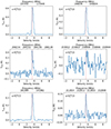 |
Fig. B.1. Observed H213CO spectra. The vertical dotted line shows the source velocity (v = 3.5 km s−1). The spin symmetry is indicated in the upper left corner of each plot, with ‘o’ standing for ortho and ‘p’ standing for para. |
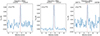 |
Fig. B.2. Observed H2C18O spectra. The vertical dotted line shows the source velocity (v = 3.5 km s−1). The spin symmetry is indicated in the upper left corner of each plot, with ‘o’ standing for ortho and ‘p’ standing for para. |
Appendix C: Sputtering yield determination: The case of a thin CO2 ice film
High-energy heavy ions irradiation of CO2 ices has been thoroughly investigated (Seperuelo Duarte et al. 2009; Mejía et al. 2015; Dartois et al. 2021). In this appendix, we compare sputtering yields estimated from the interference fringes analysis method (Method 1, as employed in this work for H2CO ice) to yields derived from the integration of IR bands (Method 2).
C.1. Method 1: Interference fringes method
The procedure follows the steps explained in Section 4.1 for H2CO ice. The interference fringes observed in the IR spectra during irradiation are depicted in Fig. C.1. The adjustments were achieved using Eq. 1. While a more rigorous equation including the optical indices could be applied in the case of CO2 (see Dartois et al. 2023, for details), we opted for the simplified equation (Eq. 1) in order to be consistent with the methodology employed in this study. The total mass sputtering yield (Ym, tot = (5.7 ± 0.1)×10−18 g ion−1) was extracted from the linear fit of surface density as a function of fluence (Fig. C.2), using a density of CO2 of 1.0 g cm−3 (Bouilloud et al. 2015). We note that in the case of CO2, there is no visible compaction phase, despite experimental conditions close to those of H2CO (similar film thicknesses, pressure and temperature, see Section 2).
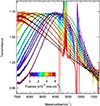 |
Fig. C.1. Infrared transmittance spectra of a CO2 ice film evolution upon 74 MeV 86Kr18+ swift heavy ion irradiation. Solid lines: Experimental data. Dashed lines: Model spectra fitted to the data, without considering the absorption bands. The QMS signal ends around a fluence of 4.1012 ion cm−2, before the end of the irradiation as the instrument stopped prematurely. |
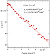 |
Fig. C.2. Evolution of the bulk mass per area as a function of fluence deduced from interference fringes for a CO2 ice film. |
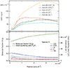 |
Fig. C.3. QMS signals as a function of fluence. Top panel: Background corrected signals. Bottom panel: Molecular fractions in the gas (solid lines, left y-axis) derived from the fragmentation patterns and ionisation cross sections, and sputtering yield of each species (dashed lines, right y-axis). See text for details. |
The CO2 fragmentation pattern was derived from the QMS signal during CO2 injection. It is composed of only four fragments at m/z = 44, m/z = 28, m/z = 16, and m/z = 12 (with intensity ratios of 0.748, 0.112, 0.07, and 0.07, respectively). Figure C.3 shows the molecular fraction deduced from the QMS signal after (i) correction of the background, (ii) extracting the original CO2 signal intensity using the fragmentation pattern (ICO2 = I(m/z = 44)/0.748), (iii) subtracting the CO2 fragments from other mass signals (e.g. IC = I(m/z = 12)−0.07 × ICO2), and (iv) dividing by the total electron-impact ionisation cross sections (σimpact(CO2) = 3.521Å2, from the NIST database ).
In contrast to H2CO, no significant variation of the CO2 fraction is observed during the very early fluences; however, a similar smooth and continuous evolution is observed thereafter. Over the entire experiment, the molecular fraction of CO increases by ∼40%, while that of CO2 decreases by ∼60%. The sputtering yields were calculated using Eq. 3 after fitting the molecular fractions with a third-order polynomial, as in the case of H2CO. The fits are shown as dashed lines in the bottom panel of Fig. C.3. The average sputtering yields are provided in Table 5.
Initial gas phase species fractions fi(X, g) and average sputtering yield YX for each species S.
As in the case of H2CO, the intact fraction of sputtered CO2 was computed using the initial fractions fi(X,g) of species containing carbon atom (Table C.1) :
We obtain η = 0.25±0.02 from which the effective sputtering yield (see Eq. 4) for a CO2 ice film was estimated as Yeff=(6.8±4.1)×104 molecules ions−1. The corresponding effective prefactor derived from Eq. 6 is Y0eff=(3.8±2.3)×10−3 1030 eV−2 cm−4 molecule3, using a stopping power of 3290 eV/1015 molecules cm−2.
C.2. Method 2: Integrated bands method
Fig. C.4 illustrates the evolution of the CO2 infrared vibrational band at 2343 cm−1 with fluence. The integrated intensity of this band (A) was employed to derive the CO2 column density (N) with the first-order relation:
where the band strength (𝒜) is 7.6 × 10⁻¹⁷ cm molecules−1 (Bouilloud et al. 2015). The derivative of the column density with respect to fluence was fitted using an equation involving both radiolysis and sputtering processes:
where σdes is the destruction cross-section of CO2, f is the relative concentration of carbon dioxide molecules with respect to the total number of molecules in the ice film, and Nd is the semi-infinite sputtering depth. Similarly to the experiment of Mejía et al. (2015) on CO2 ice irradiation, the fraction of CO2 in the ice remains significantly higher than that of CO at the observed fluences, and the value of f is set to 1. Adjusting the data with Eq. C.3, as shown in Fig. C.5, provides the following solution: Yeff = (7.0 ± 0.9)×104 molecules ions−1, σdes = (1.4 ± 0.1)×10−13 cm2 ion−1, and Nd = (1.8 ± 0.3)×1017 molecules cm−2. The derived effective sputtering yield corresponds to an effective prefator Y0eff = (6.5 ± 0.8) × 10−3 1030 eV−2 cm−4 molecule3, using again a stopping power of 3290 eV/1015 molecules cm−2.
C.3. Comparison of Method 1 and 2
Results from this work and previous studies are presented in Table C.2. The comparison with literature data is not straightforward due to various experimental conditions. For example, experiments have shown that the sputtering efficiency depends on the ice thickness: the effective sputtering yields Yeff for CO and CO2 ices were indeed found to be constant for thick films (more than ∼ 100 monolayers) but to decrease significantly for thin ice films (Dartois et al. 2021). We recall that Yeff scales with the square of the heavy ion stopping power, while Ye0 should be roughly constant for a given target. We can observe in Table C.2 that our Ye0 value derived from the integrated band method (Method 2) agrees with those of Seperuelo Duarte et al. (2009) and Dartois et al. (2021), who used the same method, to better than a factor of 2, and almost within error bars (whatever the thickness of the film). In addition, and more importantly, the interference fringes method (Method 1) gives an effective sputtering yield prefactor (Ye0 value) in very good agreement (i.e. within error bars) with the value we derived from Method 2.
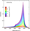 |
Fig. C.4. Evolution of the background-corrected IR spectrum centered on the ν3 stretching mode of CO2 upon 74 MeV 86Kr18+ swift ion irradiation |
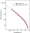 |
Fig. C.5. Column density derivative with respect to fluence. The solid and dashed lines are fits with or without including the sputtering depth Nd in Eq. C.3, respectively. |
Comparison of results for swift heavy ion irradiation of pure CO2 ice films.
We conclude that the interference fringes method, even using a simplified optical model, is a powerful alternative to the integrated bands method for the determination of sputtering yields. Furthermore, combined with QMS measurements, this method allows us to determine both effective and intact sputtering yields, this latter being challenging to estimate with other methods.
All Tables
Total electron-impact ionisation cross-sections σimpact(X); initial fractions fi(X, g) and averaged sputtering yield YX.
Initial gas phase species fractions fi(X, g) and average sputtering yield YX for each species S.
All Figures
|
Fig. 1. IR spectra of irradiated H2CO ice. Left panel: Full range spectra, corrected for baseline, with assigned spectral peaks (see Table 2). Right panel: Focus on the evolution of the four bands used to derive column density of CO2, CO, H2CO, and POM in the ice. |
| In the text | |
|
Fig. 2. Column density evolution of CO2, CO, H2CO, and POM ices as a function of fluence. In the case of POM, a factor of 2 uncertainty was assumed for the band strength of the combination mode at 1105 cm−1 (see text), as depicted by the shaded green zone. In the case of H2CO, the band strength of the stretching mode at 1725 cm−1 was also evaluated by Schutte et al. (1993) as 9.6×10⁻¹⁸ cm molecules−1 at 10 K, which corresponds to the highest column density value of the shaded red zone. Otherwise, an uncertainty of 20% was assumed for the band strengths. |
| In the text | |
|
Fig. 3. Infrared transmittance spectra of a H2CO ice film evolution as a function of fluence. Solid lines: Experimental data. Dashed lines: Model spectra fitted to the data. See text for details. |
| In the text | |
|
Fig. 4. Evolution of the surface density as a function of fluence deduced from interference fringes. The fit was performed for fluences greater than 6 × 10¹¹ ions cm−2 since the very beginning of the irradiation corresponds to ice compaction (e.g. Palumbo 2006; Dartois et al. 2013). |
| In the text | |
|
Fig. 5. QMS signals as a function of fluence. Top panel: Background corrected signals. Bottom panel: Molecular fractions in the gas (solid lines, left y-axis) derived from the fragmentation patterns and ionisation cross sections, and sputtering yield of each species (dashed lines, right y-axis). See text for details. |
| In the text | |
|
Fig. 6. Mass fragmentation pattern monitored during species injection (for ice sample deposition) for H2CO (top panel) and CO (unpublished data) (bottom panel). |
| In the text | |
|
Fig. 7. Schematic timeline of events during the first impact of a swift heavy ion (SHI) on an ice sample, within the thermal spike model. Chemistry and sputtering occur almost simultaneously within 10−9 s of the ion’s passage (Lang et al. 2020). The length ds corresponds to the sputtering depth probed by an individual ion incident, which is inferior to d0, the initial ice film thickness; rr corresponds to the radiolysis destruction radius, which is at most equal to the sputtering cylinder radius rs (Dartois et al. 2021). Considering the timescales involved, infrared spectroscopy cannot observe the radiolysis effects within the sputtered volume during the passage of an ion. |
| In the text | |
|
Fig. 8. Comparison between the observed integrated intensities (blue dots) and the integrated intensities derived from the non-LTE model (red diamonds), for each of the observed lines, labelled by their rest frequencies. In the figure, ‘o’ stands for ortho and ‘p’ stands for para. |
| In the text | |
|
Fig. 9. Intact sputtering rate of pure H2CO and effective sputtering rates of the pure ices CO, CO2, and H2O as a function of the ζ cosmic-ray ionisation rate. Effective sputtering yield pre-factors are taken from Dartois et al. (2023). |
| In the text | |
|
Fig. 10. H2CO gas phase abundance with respect to H nuclei as a function of visual extinction. The observational value derived in this study for the prestellar core L1689B (blue hatched zone) is compared to five different models for H2CO sputtering: pure H2CO ice and H2CO ideally diluted in H2O, CO2, and CO matrices. See text for details. |
| In the text | |
|
Fig. B.1. Observed H213CO spectra. The vertical dotted line shows the source velocity (v = 3.5 km s−1). The spin symmetry is indicated in the upper left corner of each plot, with ‘o’ standing for ortho and ‘p’ standing for para. |
| In the text | |
|
Fig. B.2. Observed H2C18O spectra. The vertical dotted line shows the source velocity (v = 3.5 km s−1). The spin symmetry is indicated in the upper left corner of each plot, with ‘o’ standing for ortho and ‘p’ standing for para. |
| In the text | |
|
Fig. C.1. Infrared transmittance spectra of a CO2 ice film evolution upon 74 MeV 86Kr18+ swift heavy ion irradiation. Solid lines: Experimental data. Dashed lines: Model spectra fitted to the data, without considering the absorption bands. The QMS signal ends around a fluence of 4.1012 ion cm−2, before the end of the irradiation as the instrument stopped prematurely. |
| In the text | |
|
Fig. C.2. Evolution of the bulk mass per area as a function of fluence deduced from interference fringes for a CO2 ice film. |
| In the text | |
|
Fig. C.3. QMS signals as a function of fluence. Top panel: Background corrected signals. Bottom panel: Molecular fractions in the gas (solid lines, left y-axis) derived from the fragmentation patterns and ionisation cross sections, and sputtering yield of each species (dashed lines, right y-axis). See text for details. |
| In the text | |
|
Fig. C.4. Evolution of the background-corrected IR spectrum centered on the ν3 stretching mode of CO2 upon 74 MeV 86Kr18+ swift ion irradiation |
| In the text | |
|
Fig. C.5. Column density derivative with respect to fluence. The solid and dashed lines are fits with or without including the sputtering depth Nd in Eq. C.3, respectively. |
| In the text | |
Current usage metrics show cumulative count of Article Views (full-text article views including HTML views, PDF and ePub downloads, according to the available data) and Abstracts Views on Vision4Press platform.
Data correspond to usage on the plateform after 2015. The current usage metrics is available 48-96 hours after online publication and is updated daily on week days.
Initial download of the metrics may take a while.