| Issue |
A&A
Volume 692, December 2024
|
|
|---|---|---|
| Article Number | A13 | |
| Number of page(s) | 11 | |
| Section | Galactic structure, stellar clusters and populations | |
| DOI | https://doi.org/10.1051/0004-6361/202451486 | |
| Published online | 29 November 2024 | |
The disc origin of the Milky Way bulge
The high velocity dispersion of metal-rich stars at low latitudes
1
GEPI, Observatoire de Paris, PSL Research University, CNRS,
Univ. Paris Diderot, Sorbonne Paris Cité, Place Jules Janssen,
92195
Meudon,
France
2
Leibniz-Institut für Astrophysik Potsdam (AIP),
An der Sternwarte 16,
14482
Potsdam,
Germany
3
Institute for Computational Cosmology, Department of Physics, Durham University,
Durham
DH1 3LE,
UK
4
Department of Astronomy, Astrophysics and Space Engineering, Indian Institute of Technology Indore,
Indore
453552,
India
5
Max-Planck-Institut für Astronomie,
Königstuhl 17,
69117
Heidelberg,
Germany
6
Observatoire de Paris, LERMA, Collège de France, CNRS, PSL University, Sorbonne University,
75014
Paris,
France
★ Corresponding author; This email address is being protected from spambots. You need JavaScript enabled to view it.
Received:
12
July
2024
Accepted:
20
October
2024
Abstract
Previous studies of the chemo-kinematic properties of stars in the Galactic bulge have revealed a puzzling trend. Along the bulge minor axis, and close to the Galactic plane, metal-rich stars display a higher line-of-sight velocity dispersion compared to metal-poor stars, while at higher latitudes metal-rich stars have lower velocity dispersions than metal-poor stars, similar to what is found in the Galactic disc. In this work, we re-examine this issue, by studying the dependence of line-of-sight velocity dispersions on metallicity and latitude in APOGEE Data Release 17, confirming the results of previous works. We then analyse an N-body simulation of a Milky Way-like galaxy, also taking into account observational biases introduced by the APOGEE selection function. We show that the inversion in the line-of-sight velocity dispersion-latitude relation observed in the Galactic bulge - where the velocity dispersion of metal-rich stars becomes greater than that of metal-poor stars as latitude decreases – can be reproduced by our model. We show that this inversion is a natural consequence of a scenario in which the bulge is a boxy or peanut-shaped structure, whose metal-rich and metal-poor stars mainly originate from the thin and thick disc of the Milky Way, respectively. Due to their cold kinematics, metal-rich, thin disc stars are efficiently trapped in the boxy, peanut-shaped bulge, and at low latitudes show a strong barred morphology, which – given the bar orientation with respect to the Sun-Galactic centre direction – results in high velocity dispersions that are larger than those attained by the metal-poor populations. Extremely metal-rich stars in the Galactic bulge, which have received renewed attention in the literature, do follow the same trends as those of the metal-rich populations. The line-of-sight velocity-latitude relation observed in the Galactic bulge for metal-poor and metal-rich stars are thus both an effect of the intrinsic nature of the Galactic bulge (i.e. mostly secular) and of the angle at which we observe it from the Sun.
Key words: Galaxy: bulge / Galaxy: center / Galaxy: disk / Galaxy: evolution / Galaxy: kinematics and dynamics / Galaxy: structure
© The Authors 2024
 Open Access article, published by EDP Sciences, under the terms of the Creative Commons Attribution License (https://creativecommons.org/licenses/by/4.0), which permits unrestricted use, distribution, and reproduction in any medium, provided the original work is properly cited.
This article is published in open access under the Subscribe to Open model. This email address is being protected from spambots. You need JavaScript enabled to view it. to support open access publication.
1 Introduction
The Milky Way harbours a boxy, peanut-shaped (hereafter b/p) bulge that has a stellar mass of about 2 × 10¹⁰M⊙ (Wegg & Gerhard 2013). The X-shape signature of the peanut morphology of the bulge can be seen, among other means, through the distribution of red giant stars (e.g. Ness et al. 2012; Li & Shen 2012; McWilliam & Zoccali 2010; Nataf et al. 2010; Ness & Lang 2016), whereby the two lobes that constitute the backbone of the peanut shape appear separated by about 1 kpc from the Galactic centre (GC). As several numerical works have shown, a massive classical component – a bulge that has a spheroidal structure – can be ruled out beyond a 10% contribution (Shen et al. 2010; Kunder et al. 2012; Di Matteo et al. 2014, 2015; Di Matteo 2016; Gómez et al. 2018) and the bulge is, for the most part, made of the same stellar populations found in the Galactic (thin and thick) disc, transformed to a b/p morphology via vertical resonance trapping at the bar and buckling instabilities (see the seminal works of Combes et al. 1990; Raha et al. 1991). Essentially all numerical works developed in the last decade (Shen et al. 2010; Bekki & Tsujimoto 2011; Ness et al. 2012; Ness et al. 2014; Debattista et al. 2017; Athanassoula et al. 2017; Fragkoudi et al. 2017b, 2018, 2020), when compared with data coming from large spectroscopic surveys as ARGOS (Freeman et al. 2013), BRAVA (Howard et al. 2008), GIBS (Zoccali et al. 2014), and APOGEE (Majewski et al. 2017), and with high-resolution spectroscopic observations (Bensby et al. 2010, 2011, 2013, 2014, 2017, 2020, 2021; Nandakumar et al. 2024), agree on these conclusions. These observations have indeed provided morphological, kinematic, and chemical abundance relations of bulge stars that constitute stringent constraints with which to compare formation and evolutionary scenarios.
Among these constraints, it has been shown that line-of-sight velocity dispersions (hereafter  ) for populations of stars of different metallicities reveal a surprising trend: along the minor axis and close to the Galactic plane (at latitudes |b| ≲ 5°), the most metal-rich population displays a higher
  than the most metal-poor population (Babusiaux et al. 2014; Zoccali et al. 2017; Babusiaux 2016). This is quite counter-intuitive because, in the Galactic disc, metal-poor stars, which are usually old (Fuhrmann 1998; Haywood et al. 2013; Bensby et al. 2014), had time to evolve and likely be impacted by several dynamical mechanisms (e.g. interactions with giant molecular clouds in the disc, passages and accretions of satellite galaxies), and hence tend to have a higher velocity dispersion than metal-rich stars, which are usually younger. They can also have been formed kinemat-ically hotter than stars born today. The observed inversion in trends between metal-rich and metal-poor stars observed in these central regions of our Galaxy at latitudes of |b| ≲ 5° seems to contradict this general trend. This is even more surprising given that at higher latitudes (|b| ≳ 5°) the trends are those also observed in the disc; that is, the metal-poor populations have the hottest (line-of-sight) kinematics (see, e.g., Ness et al. 2013b). This raises the question of the possibility of explaining the aforementioned trends in a scenario in which most of the bulge mass is made of disc material, reshaped by the b/p instability. If not, this would suggest a more complex nature of the Galactic bulge than that offered by numerical and theoretical models so far.
In the present work, we address this problem by analysing APOGEE Data Release 17 (DR17) observations (Abdurro’uf et al. 2022) to quantify the  -latitude relation along the Galactic bulge minor axis, for stars of different metallicities. We then compare the retrieved relation to the predictions of an N-body simulation of a Milky Way-type galaxy, in which the b/p bulge forms out of (thin and thick) disc stars, to test whether such a scenario is able to reproduce the observed trends. As we shall show, such a scenario can satisfactorily explain this apparent paradox. Indeed, because of their cold kinematics, metal-rich, thin disc stars are efficiently trapped in the b/p bulge (as shown by a number of works, see for example, Di Matteo 2016; Fragkoudi et al. 2017a; Athanassoula et al. 2017; Debattista et al. 2017; Ghosh et al. 2024) and, at low latitudes, show a strong barred morphology, which – given the bar orientation with respect to the Sun-GC direction – results in high line-of-sight velocity dispersions, larger than those attained by the metal-poor populations.
The paper is organised as follows. In Sect. 2, we describe the APOGEE DR17 data and the selection applied to construct the bulge sample used for the following analysis, as well as the N-body simulation and the mock catalogue built from it. In Sect. 3, we present the main results of this work; namely, we confirm the existence of an inversion in the  -latitude relation along the bulge minor axis, where metal-rich stars show a steeper gradient than metal-poor stars. This inversion is reproduced well by our N-body model and can be explained in terms of a differential response of metal-rich and metal-poor stars to the bar-b/p instability caused by a pre-existing difference in the kinematics of these populations. We show that this inversion strongly depends on the bar viewing angle. Finally, in Sect. 4 we summarise our results.
2 Observational data and model
2.1 Selecting bulge stars in the APOGEE catalogue
We have used stars from the APOGEE DR17 catalogue1 (Abdurro’uf et al. 2022), which provides spectroscopic quantities, such as line-of-sight velocities and chemical abundances for 647025 stars. This catalogue is complemented by the astroNN value-added catalogue (Leung & Bovy 2019), which provides distances estimated using a deep-learning approach. From this dataset, we built a bulge sample by filtering stars based on their absolute value of the X-co-ordinate2 to the GC (|X| < 1.5 kpc), relative heliocentric distance error ∆D/D < 0.2, signal-to-noise ratio (>50), and effective temperature, 3500 K< Teff < 5000 K. Finally, we cross-matched this catalogue with the APOGEE Value Added Catalogue of Galactic globular cluster stars (Schiavon et al. 2024), removing stars that have a high proba-bility3 of being globular cluster members, as we are interested in the analysis of field stars only. From our initial catalogue of 14 632 bulge stars (defined as stars within |ℓ| < 20°, |b| < 20° and |X| < 1.5 kpc), our final sample contains 5630 bulge stars.
The resulting coverage of our selected sample is shown in Fig. 1 (middle panels), and the star counts in each field in Fig. B.1 (right panels). We note that, while some fields have low counts or no stars at all, we have a denser sequence along the Galactic bulge minor axis and close to the Galactic plane at positives latitudes.
2.2 The N-body model
Data from the APOGEE catalogue were compared to a dis-sipationless N-body simulation of a Milky Way-type galaxy, originally introduced in Fragkoudi et al. (2017b), and further used in Fragkoudi et al. (2018, 2019); Khoperskov et al. (2019)4. This simulation satisfies a number of properties of the Galaxy, such as longitudinal and latitudinal metallicity gradients in the bulge, as well as metallicity distributions and their variations across the bulge extent. While we refer to Fragkoudi et al. (2018) for a comprehensive description, we recall here its main characteristics. The modelled galaxy is made of four components; namely, a thin, an intermediate, and a thick stellar disc, whose stellar densities follow Miyamoto-Nagai profiles (Miyamoto & Nagai 1975) characterised by different masses, scale lengths, and heights, reported in Table 1, as well as a dark matter halo, represented by a Plummer sphere (Plummer 1911), whose mass and characteristic radius are also reported in Table 1. The thin, intermediate, and thick discs were modelled with 5, 3, and 2 million particles, respectively, and the dark matter halo is represented by 5 million particles (see Table 1).
The initial positions and velocities were set by employing the iterative method described in Rodionov et al. (2009), by building an equilibrium phase model such that the resulting density distribution matches the constraints given by the density profiles we imposed on each component. The simulation was run using a parallel MPI Tree-code (Khoperskov et al. 2014), with the gravitational forces being computed with a tolerance parameter of θ = 0.7 and an ϵ = 50 pc softening was used. The equations of motion were integrated with a timestep, ∆t = 0.2 Myr.
The thin disc is associated with a metal-rich ([Fe/H] > 0) and kinematically cold initial population of stars (referred to as Dl in the original paper), the intermediate disc is associated with an intermediate metallicity (−0.5 < [Fe/H] < 0) and intermediate initial velocity dispersion population (D2), and the thick disc is associated with a metal-poor ([Fe/H] < −0.5) and kinematically hot initial population (D3), and thus mimics the main properties of the Galactic disc (see Haywood et al. 2013). In particular, the scale heights and scale lengths of these three discs are compatible with the findings by Bovy et al. (2012), even if here we discretise, with three components only, a disc where populations of different metallicities have a more continuous distribution. Disc particles were assigned a metallicity by drawing randomly from a normal distribution, where each disc has a constant (i.e. without any radial or vertical metallicity gradient within each component) mean metallicity and dispersion (see Table 1).
The simulation was evolved for 7 Gyr, well after the bar (t = 0.5 Gyr) and b/p bulge (t = 5 Gyr) formed, and in this work we have analysed one of its last snapshots, at t = 7 Gyr. In order to make a proper comparison with the observational data, we re-scaled the positions of this final snapshot by a factor of 0.5, so that the semi-major axis of the simulated bar has a length of 5 kpc, which is compatible with observations (Wegg et al. 2015). We consequently also re-scaled the masses, and time, to preserve the virial equilibrium of the system. To build the Galactic frame as well as to compute line-of-sight velocities, the Sun was placed along the X axis, at a distance of 8.12 kpc from the centre of the simulated galaxy, and at an angle of 27° with respect to the bar, so as to match the position of the Sun relative to the centre of the Milky Way (Babusiaux & Gilmore 2005; Wegg & Gerhard 2013; Wegg et al. 2015; Chatzopoulos et al. 2015; Reid et al. 2014; Cao et al. 2013; Rattenbury et al. 2007; Stanek et al. 1997; López-Corredoira et al. 2005). The density maps of the analysed snapshot are reported in Fig. 1 (left panels), where projections both on the galaxy plane and in galactic co-ordinates are shown.
Finally, similarly to Fragkoudi et al. (2018), to make a robust comparison of the model to the observational data, we take into account the APOGEE selection function by imposing the APOGEE (heliocentric) distance distribution function (DDF), along different lines of sight, on the model. The details of the procedure adopted to reproduce the DDF for each line of sight are described in Appendix B, and the resulting mock catalogue, where the simulation has been convolved with the APOGEE DDF, is shown in Fig. 1, for the projection on the Galactic plane (X–Y) and in (ℓ – b) co-ordinates (top and bottom panels, respectively).
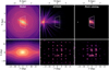 |
Fig. 1 Density maps of the N-body simulation stars (left column), APOGEE stars (middle column), and our mock catalogue stars (right column). Top panel: face-on maps (X-Y-plane), with |X| < 1.5kpc distance bounds and ±20° longitude bounds in white, as well as a green line to guide the eye, indicating the angle of the Galactic bar and the Sun at X = −8.12 kpc,Y = 0 kpc (white star symbol). Bottom panels: corresponding maps in the Galactic (ℓ,b) plane. The colours indicate relative densities for each of the three catalogues separately. |
Initial parameters for each of the components of the N-body simulation used in this work.
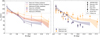 |
Fig. 2 Line-of-sight velocity dispersion, |

3 Results
3.1 Comparing APOGEE DR17 and literature data with the N-body model
In Fig. 2 (left panel), the velocity dispersion profiles of metal-rich ([Fe/H] ≥ 0), metal-intermediate (−0.5 ≤ [Fe/H] < 0), and metal-poor ([Fe/H] < −0.5) populations along the bulge minor axis are shown, for the N-body model and the APOGEE data. In both cases, we have selected only stars with longitudes of |ℓ| < 2° and with a galactocentric co-ordinate, |X| < 1.5 kpc. To construct the velocity dispersion profiles from the simulation, we have applied the APOGEE DDF to the model, as was mentioned in the previous section, and as is described more in detail in Appendix B. As for the APOGEE data, we selected bulge stars using the criteria described in Sect. 2.1. Both in the observational and simulated data, we used a wide latitude binning to mitigate low star counts by grouping neighbouring fields (where we used the following latitude ranges for the bins : ([0º,2º], [2º,4º], [4º,7º], [7º,9º], [9°,13°], [13°,17°], and [17°,19°]), and uncertainties in the velocity dispersion profiles were computed via a bootstrapping method.
Comparing the velocity dispersion profiles along the bulge minor axis of metal-rich, metal-intermediate, and metal-poor stars obtained by analysing the APOGEE bulge sample (solid lines in Fig. 2, left panel), it is evident that for |b| ≳ 5° the trend with metallicity is such that the lower the metallicity, the higher the velocity dispersion, as is expected if stars in these metallicity ranges arise from populations whose kinematics becomes hotter with decreasing metallicity (and as is shown by the profiles at t = 0 Gyr in Appendix A, where the discs are still in their initial conditions and no bar or bulge has formed). At |b| < 5° the trend is reversed, and the metal-poor populations become the kinematically coolest. The N-body simulation shows the same trend: while at high absolute latitudes (|b| > 5°) the metal-rich stars are, among the three populations analysed, those characterised by the lowest line-of-sight velocity dispersions, as |b| diminishes, they become the hottest population, by reaching συlos ~ 160 km s−1 close to the Galactic mid-plane.
In Fig. 2 (right panel), we compare the dispersion profiles resulting from the APOGEE bulge sample, and from our mock catalogue, with the velocity dispersion profiles along the bulge minor axis obtained by previous works. In this figure, stellar particles of the N-body simulation have been divided into two groups only, metal-rich ([Fe/H] ≥ 0) and metal-poor ([Fe/H] < −0.5), and are compared with data from the literature, where often bulge stars are grouped into two components only (but see Ness et al. 2013b, for a finer subdivision of the metallicity range). Literature data points have been extracted from Babusiaux (2016) (and are originally from Babusiaux et al. 2010; Babusiaux et al. 2014; Ness et al. 2013b; Rojas-Arriagada et al. 2014; Uttenthaler et al. 2012), to which we added data from Zoccali et al. 2017.
In general, we see that the results obtained by analysing the APOGEE data are, within the uncertainties, in agreement with previous works: close to the Galaxy midplane, metal-rich bulge stars have a higher line-of-sight velocity dispersion than metal-poor stars, and a clear inversion to this trend is seen for |b| ≥ 5°. As a result of this inversion, the slope of the συlos − |b| relation for metal-rich stars is steeper than that of the metal-poor stars: for |b| ≤ 7.5°, where most of the observational data are found, the two slopes are, respectively, −15.99 ± 1.39 km s−1 deg−1 and −8.07 ± 2.27 km s−1 deg−1. In the same latitude range, the slopes found in the simulations are similar, with −10.62 ± 0.15 km s−1 deg−1 for metal-rich stars and −7.33 ± 0.05 km s−1 deg−1 for metal-poor stars. We mention that, in calculating these slopes, we have given a similar weight to all observational data points, despite the fact that they do not all use the same definition for metal-rich and metal-poor stars (while the compilation of Babusiaux (2016) adopts a separation at 0 < [Fe/H] < 0.5 and at −1 < [Fe/H] < −0.5, respectively, Zoccali et al. (2017) adopts a slightly different definition for metal-rich stars ([Fe/H] > 0.1 in their work) and a broader interval for metal-poor stars ([Fe/H] < −0.1)5). Despite the differences in the definitions of the two groups, as well as the use of different distance estimates for stars in the analysed samples, the different trends in the kinematics of the two groups are visible. Indeed, the fact that they are present irrespective of the details of the analysis (i.e. metal-licity range, distance estimates, amplitude of the longitude and latitude intervals) strengthens the robustness of these findings.
Finally, it is worth citing in this context some new results about the presence of extremely metal-rich stars in the Galactic bulge, whose existence has been known for some time (see, for example, Fulbright et al. 2006; Johnson et al. 2007; Zoccali et al. 2008). Rix et al. (2024) recently suggested that this population forms a dynamically hot system, a ‘knot’, in the inner 1.5 kpc of our Galaxy (see also Horta et al. 2024). While we defer a specific study of these stars to future works, it is nevertheless interesting, in the context of the present paper, to investigate the συlos-|b| relation that they trace, because the latter helps to constrain their nature. To this aim, in Fig. 3, we have split the APOGEE metal-rich bulge population into two groups, made, respectively, of 277 stars with 0 < [Fe/H] ≤ 0.3 (hereafter called very metal-rich (VMR) stars), and of 272 stars with 0.3 < [Fe/H] (hereafter called extremely metal-rich (EMR) stars). The figure shows that these groups share the same συlos-|b| relation, which points to the fact that: 1) at low latitudes, EMR stars are as dynamically hot (in line-of-sight projection) as VMR stars, and as the metal-rich population as a whole; 2) similarly to VMR stars, the EMR population shows a steep συlos-|b| gradient, with συlos = 55 km s−1 at |b| ~ 10 °, and rising up to συlos = 170 km s−1 at |b| < 2 °. These findings suggest that, in terms of line-of-sight kinematics, EMR stars are not exceptional, but share the same kinematic behaviour as the bulk of the metal-rich population (0 < [Fe/H] < 0. 3). We note that the choice of separating VMR and EMR at a 0.3 dex metallicity was done to maximise the number of EMR stars, which rapidly decreases with increasing metallicity, and thus our choice of definition of VMR and EMR stars does not exactly match the one made in Rix et al. (2024).
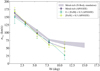 |
Fig. 3
|

3.2 Understanding the inversion in the line-of-sight velocity dispersions at low latitudes
The comparison of observational data with the N-body simulation presented in the previous section shows that even a model in which bulge populations with [Fe/H] ≥ −1 originate exclusively from disc stars is able to reproduce the observations, and in particular the apparent ‘dual’ nature of the metal-rich population, which is kinematically hot at low latitudes and kinematically cold at higher latitudes. As a further step, we need to understand why, in the model, bulge metal-rich stars – originally belonging to the kinematically coldest disc (i.e. D1) – end up showing the largest line-of-sight velocity dispersions at low latitudes.
To this aim, in Fig. 4 we show the maps of the velocity dispersion of metal-rich, metal-intermediate, and metal-poor stellar particles of the N-body model, projected on the galaxy midplane, for two different values of the dispersion measured, respectively, along the in-plane bulge major ( , left panels) and in-plane minor (
 , right panels) axis. In this figure, we have chosen a galactocentric reference frame in which the xb axis is parallel to the bar major axis, and the Yb axis is perpendicular to it, with both axes lying on the galaxy midplane. Different rows in Fig. 4 show different slices in height from the midplane for stars in the three metallicity intervals at, respectively, |Z| ≤ 0.25 kpc (|b| ≤ ~1.8° at the GC), 0.25 kpc< |Z| ≤ 0.5 kpc (~1.8°≤ |b| ≤ ~3.6° at the GC), and 0.5 kpc< |Z| ≤ 1 kpc (~3.6°≤ |b| ≤ ~7.1° at the GC). Density contours are also reported in all the plots to link kinematic properties to morphological features. Similar maps, but in the (ℓ, b) plane and for a Sun-Galactic Bar angle of 27°, are shown in Appendix D.
As for the morphological properties, from this figure we can see that:
The b/p structure is visible at larger heights above the plane (0.5 < |Z| ≤ 1 kpc) as a double-lobe feature, or split, in the density contours. At these heights above the plane, this feature is stronger for the metal-rich population and weaker for the metal-intermediate one, and absent for the metal-poor one. The b/p structure disappears at smaller |Z|. These trends are all qualitatively similar to those found in other N-body simulations (among others, see Fragkoudi et al. 2017a, 2018), as well as in observational data, where the presence of the b/p structure is traced, for instance, by the split in the distribution of red clump stars (see, e.g. Ness et al. 2013a,b).
-
Apart from the double-lobe feature in some of the isodensity contours, most of them appear nearly elliptical, the elliptic-ity being higher for the metal-rich population than for the metal-poor one (see Appendix C for more details on this point). This difference in ellipticity of the isodensity contours reflects a difference in the strength of the bar, as traced by metal-rich, metal-intermediate, and metal-poor populations, in agreement with a number of previous studies (see Babusiaux et al. 2010; Fragkoudi et al. 2017a; Debattista et al. 2017; Bekki & Tsujimoto 2011; Athanassoula 2003; Combes et al. 1990).
As for the kinematic properties, we can see that:
The structure and amplitude of the maps of the velocity dispersion along the bar major axis
 vary both as a function of metallicity and height above the plane.
Close to the galaxy midplane (|Z| ≤ 0.25 kpc), metal-rich stars show velocity dispersions with a butterfly-like pattern, characterised by high values (greater than 140 km s−1 ) over most of the inner 1.5 kpc region of the simulated galaxy. At |Z| < 0.25 kpc, the intermediate population shows the lowest values of
 , while the metal-poor population has
  values similar to that of the metal-rich one, but extended over a more limited region than the metal-rich particles (compare the spatial extension of the red-brown region in the left and right columns of Fig. 4, left panels).
At higher distances from the galactic plane, in the innermost few hundred parsecs from the galaxy centre, the metal-rich population sustains a higher
 than the metal-intermediate and metal-poor populations whose central velocity dispersion decreases with|Z|. However, except for this innermost region, one sees that, overall, the
  values are larger for the metal-intermediate and metal-poor stars than for the metal-rich ones (while the former have
  of about 100 km s−1 inside most of the region delimited by R = 1.5 kpc, the
  of the metal-rich population rapidly decreases to values as low as ~80 km s−1 in the same spatial region).
The velocity dispersions perpendicular to the bar major axis (
 , see Fig. 4, right panels) show a different behaviour, with the metal-rich population always being colder than the metal-intermediate and metal-poor ones, at low vertical distances as well as at large vertical distances to the galaxy midplane.
From these findings, we can understand that the asymmetry in the mass distribution of the inner disc regions (bar and b/p bulge) is also accompanied, in these same regions, by an asymmetry in the kinematics of the stars. The velocity dispersion generally has a higher intensity along the major axis of the bar than along the direction perpendicular to it (i.e. implying velocity dispersion maps that are also asymmetrical). Its intensity also varies with the metallicity of the stellar population, and this trend is a natural consequence of a bar formed from a disc in which a pre-existing relation between the metallicity of the stars and their velocity dispersion, similar to that observed in the Galactic disc (e.g. Bovy et al. 2012; Haywood et al. 2013), was in place. In this case, as has been discussed in previous works, kinematically colder and thinner stellar discs produce stronger bars with greater ellipticity than kinematically hotter and thicker discs (Bekki & Tsujimoto 2011; Fragkoudi et al. 2017a; Athanassoula et al. 2017; Debattista et al. 2017; Ghosh et al. 2023).
The results presented in Fig. 4 have a natural consequence: the line-of-sight velocity dispersion of stars in a bar-b/p structure changes with the viewing angle. To further address this point, in Fig. 5 we show the  relation for metal-rich ([Fe/H] > 0), metal-intermediate (−0.5 < [Fe/H] < 0), and metal-poor ([Fe/H] < −0.5) particles, in the cases of a simulated bar observed end-on (i.e. the line-of-sight being parallel to the bar major axis and the bar viewing angle being equal to 0°), side-on (i.e. the line-of-sight being perpendicular to the bar major axis and the bar viewing angle being equal to 90°) and at intermediate angles of 45° and 70°. The variation of
  with latitude significantly changes in the four cases, as is anticipated from Fig. 4. If the bar is viewed side-on, the resulting line-of-sight velocity dispersion has a monotonic trend with metallicity, at all |b|, with the bulge metal-rich population having lower values
  than the bulge metal-poor population, at all latitudes. If the orientation of the bar angle is intermediate (45°), an inversion in the
  values for metal-rich and metal-poor components starts to appear at |b| ~ 5°. When the bar is viewed end-on, the
  of the metal-rich population at |b| ~ 2–5° is definitely higher than that of more metal-poor stars. Interestingly, at |b| ≲ 2°, a drop in the line-of-sight velocity dispersion of metal-rich stars is predicted by our N-body model. The origin of this feature needs further investigation, which requires higher-resolution simulations than the one presented in this paper. We note that in Fig. 5 we used all particles of the N-body simulation without any sampling or convolution with DDF, since in this figure we are not comparing the model with any observational data. Profiles made with continuously increasing bar-observer (i.e. Sun) position angles between 0 and 90° show a continuous trend of metal-rich stars becoming hotter close to the plane (with the specific configuration of an observer placed at an angle of ~27º relative to the Galactic bar being represented in Fig. 2). This certainly does not suggest that the kinematics of the populations inherently change with the position of the observer, but rather that the velocity dispersions we are referring to are measured through the line-of-sight component.
We interpret this dependence of the dispersion inversion on the Sun-Galactic bar orientation as follows: at low angles, the line-of-sight velocities in the innermost regions of the bulge are mainly dominated by the υXb component of velocities, the component along the major axis of the bar. As the dispersion maps in Fig. 4 show, the metal-rich population displays a wider region of high  dispersion than the metal-poor population. Hence, at low Sun-Galactic bar angles, we expect the line-of-sight velocity dispersion profiles to reflect the difference in
  dispersions. At angles closer to 90°, however, the line-of-sight velocity is mainly dominated by the υYb component (perpendicular to the bar major axis), for which the dispersion maps show higher dispersion for metal-poor stars than for metal-rich ones. Thus, the right panel of Fig. 5 shows no or a very weak dispersion inversion between the metal-rich and metal-intermediate stars. This can also be seen in the dispersion maps of Fig. 4, for the
  component. Indeed, we observe, at low|Z| (top panels), that the metal-rich and metal-intermediate populations display similar patterns of dispersion in their central regions. At higher latitudes (|b| > 5°), we find that the trends do not depend on the Sun-bar angle anymore but rather display the expected result of the metal-poor population being kinematically hotter than the metal-rich one. In fact, dispersion maps at higher Z-slices show that the dispersion patterns seen in Fig. 4 near the Galactic plane are not present at high altitudes, highlighting the fact that the dispersion inversion is a near-Galactic plane effect of the kinematics of each components. Paradoxically, it is the fact that the metal-rich population is kinematically colder than the metal-poor population that causes it to be more efficiently trapped in Galactic plane-bound and eccentric orbits, and thus leads to a higher line-of-sight velocity dispersion being generated at low latitudes.
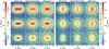 |
Fig. 4 Maps of the velocity dispersion maps for the bar-oriented |


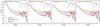 |
Fig. 5 Line-of-sight velocity, |

3.3 Limitations of the N-body model and possible effects on the συlos -|b| relation
The N-body model with which observational data are compared lacks at least two ingredients that may have an impact on the συlos-lbl relation.
A gaseous disc, and associated star formation. In our N-body model, the whole thin disc is present since the beginning of the simulation, and thus does not form stars over time. As a consequence, metal-rich, thin disc stars all have the same velocity dispersion, before the bar and b/p bulge form. The presence of ongoing star formation and the birth of young stellar populations over time should have the consequence of reducing the velocity dispersion of the disc, possibly counteracting its kinematic heating over time. In the comparison shown in Fig. 2 (left and right panels), metal-rich particles in the N-body simulation tend to have a slightly higher συlos -|b| than in the APOGEE data, at |b| ≳ 5°. We shall investigate in future works whether the reason of this difference – which is within 1–2 σ from the data – may be due to a lack of continuous star formation in the model.
A stellar halo. A number of studies have shown that the stellar halo of the Milky Way is composite (e.g. Nissen & Schuster 2010; Haywood et al. 2018; Di Matteo et al. 2019; Belokurov et al. 2020; Naidu et al. 2020; Horta et al. 2023), with an accreted and an in situ population, both of which are kinematically hotter than the Galactic thin and thick discs. Even if the stellar halo is a tiny fraction of the total stellar mass budget in the Galaxy, halo stars with [Fe/H] > −1 in the inner regions of the Milky Way may contribute to increasing the overall velocity dispersions of the most metal-poor components, and thus, in particular, their συlos. The comparison made in Fig. 2 (left panel) between the APOGEE data and the N-body simulation shows that the former tend to show a higher συlos than the latter, at all latitudes |b| > 5°. It is, however, premature to ascribe this difference to the absence of a halo component in the simulation, which may, in turn, affect the observational estimates. Indeed, Figure 2 (right panel) shows that the difference between the N-body model and the APOGEE data is of the same order as the difference found between APOGEE data and other observational studies (see, for example, Ness et al. 2013b; Zoccali et al. 2017).
Finally, the reader may have noted that no classical bulge is included in this simulation. As was recalled in the introduction, several works have shown that – if present – a classical bulge should represent a few percent of the stellar mass of the Milky Way (so, typically, a few 10° M⊙) and no more than one tenth (so ~5 × 10⁹ M⊙). Shen & Zheng (2020) discussed the incompatibility of the presence of a massive classical bulge in the centre of the Milky Way with the observations of a distinct nuclear star cluster, which would have been impossible to detect were this classical bulge significantly massive. Such a classical component, according to the mass-size relations of spheroids (e.g. see Hon et al. 2023, their Fig. 4), should have an effective radius of less than 200 pc at most, which translates into an angular size of 1.4° at the distance of the GC. So, even if it were present, this classical component would have no effect on the inversion observed at b ~ 5° in the συlos-|b| relation. Its presence may affect the velocity dispersion of the most metal-poor stars in our analysis (because of the existence of a mass-metallicity relation for spheroids, classical bulges of 108 – 109M⊙ would have a typical mean metallicity between −1 and −0.5 dex, see Kirby et al. 2013; Domínguez-Gómez et al. 2023) only in the innermost 1-2 degrees of the Galaxy. In this respect, it may be interesting to investigate to what extent such a small, metal-poor component can affect the συlos at low latitudes, and – by making use of the comparison with observational data – finally prove (or disprove) its presence in the inner Milky Way.
4 Conclusions
In this work, we have made use of APOGEE DR17 data to derive the line-of-sight velocity dispersion of stars along the bulge minor axis (i.e. as a function of latitude b) for different metallicity bins. Our results confirm previous works (Babusiaux et al. 2014; Babusiaux 2016; Rojas-Arriagada et al. 2014; Zoccali et al. 2017) about the existence of an inversion in the amplitude of the line-of-sight velocity dispersion of metal-rich and metal-poor stars, with the former having a higher dispersion at |b| < 5° than metal-poor stars. We analysed a previously developed N-body simulation where the bar-b/p structure forms out of a disc, where metal-rich stars are distributed in a thin disc, and metal-poor stars in a thicker disc component. This allowed us to demonstrate that the trends observed in the observational data are a natural consequence of the differential mapping of kinematically cold and hot disc populations into a bar and b/p bulge. Metal-rich, thin disc stars are trapped efficiently in the bar instability, which results in high velocity dispersions along the bar major axis, especially close to the Galaxy midplane. A steep velocity dispersion gradient (−15.99 ± 1.39 km s−1 deg−1 in the observational profile, and −10.62 ± 0.15 km s−1 deg−1 in the profile from our simulation) is found for this population. Metal-poor, thick disc stars, in turn, show a hot kinematics trend at all latitudes, which results in a flatter gradient with latitude b. The consequence of this different response to the bar and b/p bulge results in a metal-rich component that appears kinematically hotter (along the line of sight) than the metal-poor one. Overall, the line-of-sight velocity dispersion-latitude relations observed in the Galactic bulge for metal-poor and metal-rich stars are both an effect of the intrinsic nature of the Galactic bulge (i.e. mostly secular) and of the angle at which we observe it from the Sun.
In this context, we emphasise that extremely metal-rich stars (see also Rix et al. 2024), defined in this work as stars with [Fe/H] > 0.3, show the same line-of-sight velocity dispersion-latitude relation as that of the metal-rich stars with less extreme metallicities (i.e. stars with 0 < [Fe/H] < 0.3). In terms of line-of-sight kinematics, these stars are thus not exceptional, but share the same behaviour as the majority of metal-rich stars. This suggests that, as the bulk of the metal-rich population, extremely metal-rich stars are also part of the bar. As for the metal-rich population as a whole, the characteristics of their line-of-sight velocity dispersion-latitude relation (steep increase in  with decreasing latitude, and high values of
  close to the Galactic midplane) suggest that these stars were born in a dynamically cold population and were then trapped in the bar instability.
More generally, with this work we confirm that a scenario in which most of the mass in the Galactic bulge (i.e. at [Fe/H] > −1) formed out of disc material, where metal-rich and metal-poor populations coexisted and were characterised by different kinematics (the lower the metallicity, the higher the velocity dispersion) is able to reproduce all the trends observed in the Galactic bulge, from the split in the red clump distribution and its dependence on metallicity (Ness et al. 2012; Li & Shen 2012; Fragkoudi et al. 2017a; Debattista et al. 2017), to the metallicity distributions and their change with longitude and latitude across the bulge region (Fragkoudi et al. 2017b, 2018). Together with the existence of an extended age range for stars in the bulge (Bensby et al. 2013; Ness et al. 2014; Dékány et al. 2015; Haywood et al. 2016), our results allow for an even more robust anchoring of the origin of the Galactic bulge to that of the stellar populations in the inner disc.
Acknowledgements
We thank the anonymous referee for useful comments which helped to improve this paper. This work has made use of the computational resources obtained through the DARI grant A0120410154 (PI: P. Di Matteo). This work has used data from the APOGEE DR17 catalogue. Funding for the Sloan Digital Sky Survey IV has been provided by the Alfred P. Sloan Foundation, the U.S. Department of Energy Office of Science, and the Participating Institutions. SDSS acknowledges support and resources from the Center for High-Performance Computing at the University of Utah. The SDSS website is www.sdss4.org. SDSS is managed by the Astrophysical Research Consortium for the Participating Institutions of the SDSS Collaboration including the Brazilian Participation Group, the Carnegie Institution for Science, Carnegie Mellon University, Center for Astrophysics I Harvard & Smithsonian (CfA), the Chilean Participation Group, the French Participation Group, Instituto de Astrofísica de Canarias, The Johns Hopkins University, Kavli Institute for the Physics and Mathematics of the Universe (IPMU) / University of Tokyo, the Korean Participation Group, Lawrence Berkeley National Laboratory, Leibniz Institut für Astrophysik Potsdam (AIP), Max-Planck-Institut für Astronomie (MPIA Heidelberg), Max-Planck-Institut für Astrophysik (MPA Garching), Max-PlanckInstitut für Extraterrestrische Physik (MPE), National Astronomical Observatories of China, New Mexico State University, New York University, University of Notre Dame, Observatório Nacional / MCTI, The Ohio State University, Pennsylvania State University, Shanghai Astronomical Observatory, United Kingdom Participation Group, Universidad Nacional Autónoma de México, University of Arizona, University of Colorado Boulder, University of Oxford, University of Portsmouth, University of Utah, University of Virginia, University of Washington, University of Wisconsin, Vanderbilt University, and Yale University. The following python libraries were used for this study: Astropy (Astropy Collaboration 2013, 2018, 2022), scipy (Virtanen et al. 2020), numpy (Harris et al. 2020) and matplotlib (Hunter 2007).
Appendix A Dispersion profiles for the initial conditions
In Fig. A.1 we show  profiles, similarly to Fig. 2, but for the metal-rich, metal-intermediate and metal-poor stars after setting the initial conditions of the simulation, that is at time t=0 Gyr. The profiles were computed using bootstrapping, and the hatched areas show the uncertainties associated with the stochastic sampling and the propagated uncertainties caused by the procedure of building a mock catalogue, as described in Appendix B. At latitudes |b| ≳ 10°, the metal-rich profile displays high uncertainties, on account of the low star count at heights greater than the scale height of the associated thin disc. The inversion effect is absent from the initial profiles as the velocity dispersion is simply inversely correlated with metallicity. The formation of the b/p bulge generates the dispersion inversion effect seen in the profiles of Fig. 2, and in the solid lines of Fig. A.1, at low latitudes. At higher latitudes, the profiles are left unchanged.
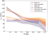 |
Fig. A.1 Line-of-sight velocity dispersion, |

Appendix B Building a mock catalogue
To compare dispersion profiles built with observational data from APOGEE DR17, we created a mock catalogue from our N-body simulation, taking into account observation biases. We first used APOGEE distance uncertainties to scatter the simulation particles along their respective (ℓ,b) direction in order to input a ‘measure-caused’ scatter in our model. We then computed DDFs in each (ℓ,b) direction for the APOGEE bulge stars, and sampled our model particles in such a way that the resulting DDFs reproduce the observational DDFs. In practice, building DDFs is not straightforward as some directions have low star counts; therefore, we used distance uncertainties to smooth the DDFs, making the sampling of our model particles more resilient to low statistics. The star count along each direction is shown in Fig. B.1, where low statistic fields (star counts < 25) are displayed in red. Stars with a globular cluster membership probability higher than 90% have been excluded and are plotted as triangle symbols. While many fields seem to fall in the low-statistics category, we point out that the star counts sequence along the minor axis near ℓ=0° – which is the region of interest for our analysis – is relatively high (especially at positive latitudes), up to b = 17°. As can be seen from the middle panel of Fig. 1, strong selection biases produce a sparse cover of the (ℓ, b) plane.
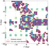 |
Fig. B.1 Star count map of our quality sample of APOGEE stars in the Galactic (ℓ,b) plane. Low-star count regions where no DDF can be constructed are painted in red, and globular clusters stars excluded from our sample are marked with triangle symbols. |
Appendix C Measuring the eccentricity of the bar isodensity contours
To quantify the morphological differences between the structures sustained by different populations of stars, we measured the bar strength for the metal-rich and metal-poor components. To this end, we used a standard Fourier coefficient Am method, computed as follows:

where the m = 0 mode is simply the number of particles N, and the m = 2 mode is a measure of the dipolarity of our sample. With this method, we also have access to the angle of the galactic bar Φ, as Φ = atan(b/a2)/2. We measure a constant 46 km s−1 kpc−1 bar pattern speed value in the last 1 Gyr. We computed the Fourier coefficients for rings of increasing radii around the GC, and we plot the results against each radius in Fig. C.2, for the metal-poor population in orange and the metal-rich population in purple. We find that the bar strength of metal-rich stars is consistently stronger than their metal-poor counterpart. Figure C.1 shows the density maps of the metal-rich and metal-poor components for the last snapshot of the simulation. We observe the same overall difference: the metal-rich population having a stronger bar signature than the metal-poor population.
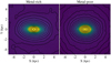 |
Fig. C.1 Density maps for the metal-rich (left panel) and for the metal-poor (right panel) population, represented in a bar-aligned reference frame and normalised by the number of particles in each component (D1 and D3). Isodensity contours are added as solid lines. |
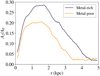 |
Fig. C.2 Bar strength of the metal-rich population (purple curve) and metal-poor population (orange curve) against mean radius, as measured by the ratio of the A2/A0 Fourier coefficients. |
Appendix D Dispersion maps in the (ℓ,b) plane
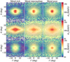 |
Fig. D.1 (ℓ,b) maps of the velocity dispersion συ maps for the bar-oriented |


References
- Abdurro’uf, Accetta, K., Aerts, C., et al. 2022, ApJS, 259, 35 [NASA ADS] [CrossRef] [Google Scholar]
- Astropy Collaboration (Robitaille, T. P., et al.) 2013, A&A, 558, A33 [NASA ADS] [CrossRef] [EDP Sciences] [Google Scholar]
- Astropy Collaboration (Price-Whelan, A. M., et al.) 2018, AJ, 156, 123 [Google Scholar]
- Astropy Collaboration (Price-Whelan, A. M., et al.) 2022, ApJ, 935, 167 [NASA ADS] [CrossRef] [Google Scholar]
- Athanassoula, E. 2003, MNRAS, 341, 1179 [Google Scholar]
- Athanassoula, E., Rodionov, S. A., & Prantzos, N. 2017, MNRAS, 467, L46 [Google Scholar]
- Babusiaux, C. 2016, PASA, 33, e026 [NASA ADS] [CrossRef] [Google Scholar]
- Babusiaux, C., & Gilmore, G. 2005, MNRAS, 358, 1309 [NASA ADS] [CrossRef] [Google Scholar]
- Babusiaux, C., Gómez, A., Hill, V., et al. 2010, A&A, 519, A77 [NASA ADS] [CrossRef] [EDP Sciences] [Google Scholar]
- Babusiaux, C., Katz, D., Hill, V., et al. 2014, A&A, 563, A15 [NASA ADS] [CrossRef] [EDP Sciences] [Google Scholar]
- Bekki, K., & Tsujimoto, T. 2011, MNRAS, 416, L60 [NASA ADS] [CrossRef] [Google Scholar]
- Belokurov, V., Sanders, J. L., Fattahi, A., et al. 2020, MNRAS, 494, 3880 [Google Scholar]
- Bensby, T., Feltzing, S., Johnson, J. A., et al. 2010, A&A, 512, A41 [NASA ADS] [CrossRef] [EDP Sciences] [Google Scholar]
- Bensby, T., Adén, D., Meléndez, J., et al. 2011, A&A, 533, A134 [NASA ADS] [CrossRef] [EDP Sciences] [Google Scholar]
- Bensby, T., Yee, J. C., Feltzing, S., et al. 2013, A&A, 549, A147 [NASA ADS] [CrossRef] [EDP Sciences] [Google Scholar]
- Bensby, T., Feltzing, S., & Oey, M. S. 2014, A&A, 562, A71 [NASA ADS] [CrossRef] [EDP Sciences] [Google Scholar]
- Bensby, T., Feltzing, S., Gould, A., et al. 2017, A&A, 605, A89 [NASA ADS] [CrossRef] [EDP Sciences] [Google Scholar]
- Bensby, T., Feltzing, S., Yee, J. C., et al. 2020, A&A, 634, A130 [NASA ADS] [CrossRef] [EDP Sciences] [Google Scholar]
- Bensby, T., Gould, A., Asplund, M., et al. 2021, A&A, 655, A117 [NASA ADS] [CrossRef] [EDP Sciences] [Google Scholar]
- Bovy, J., Rix, H.-W., Liu, C., et al. 2012, ApJ, 753, 148 [Google Scholar]
- Cao, L., Mao, S., Nataf, D., Rattenbury, N. J., & Gould, A. 2013, MNRAS, 434, 595 [NASA ADS] [CrossRef] [Google Scholar]
- Chatzopoulos, S., Fritz, T. K., Gerhard, O., et al. 2015, MNRAS, 447, 948 [Google Scholar]
- Combes, F., Debbasch, F., Friedli, D., & Pfenniger, D. 1990, A&A, 233, 82 [NASA ADS] [Google Scholar]
- Debattista, V. P., Ness, M., Gonzalez, O. A., et al. 2017, MNRAS, 469, 1587 [Google Scholar]
- Dékány, I., Minniti, D., Majaess, D., et al. 2015, ApJ, 812, L29 [CrossRef] [Google Scholar]
- Di Matteo, P. 2016, PASA, 33, e027 [CrossRef] [Google Scholar]
- Di Matteo, P., Haywood, M., Gómez, A., et al. 2014, A&A, 567, A122 [NASA ADS] [CrossRef] [EDP Sciences] [Google Scholar]
- Di Matteo, P., Gómez, A., Haywood, M., et al. 2015, A&A, 577, A1 [NASA ADS] [CrossRef] [EDP Sciences] [Google Scholar]
- Di Matteo, P., Haywood, M., Lehnert, M. D., et al. 2019, A&A, 632, A4 [NASA ADS] [CrossRef] [EDP Sciences] [Google Scholar]
- Domínguez-Gómez, J., Pérez, I., Ruiz-Lara, T., et al. 2023, A&A, 680, A111 [NASA ADS] [CrossRef] [EDP Sciences] [Google Scholar]
- Fragkoudi, F., Di Matteo, P., Haywood, M., et al. 2017a, A&A, 606, A47 [NASA ADS] [CrossRef] [EDP Sciences] [Google Scholar]
- Fragkoudi, F., Di Matteo, P., Haywood, M., et al. 2017b, A&A, 607, L4 [NASA ADS] [CrossRef] [EDP Sciences] [Google Scholar]
- Fragkoudi, F., Di Matteo, P., Haywood, M., et al. 2018, A&A, 616, A180 [NASA ADS] [CrossRef] [EDP Sciences] [Google Scholar]
- Fragkoudi, F., Katz, D., Trick, W., et al. 2019, MNRAS, 488, 3324 [NASA ADS] [Google Scholar]
- Fragkoudi, F., Grand, R. J. J., Pakmor, R., et al. 2020, MNRAS, 494, 5936 [Google Scholar]
- Freeman, K., Ness, M., Wylie-de-Boer, E., et al. 2013, MNRAS, 428, 3660 [NASA ADS] [CrossRef] [Google Scholar]
- Fuhrmann, K. 1998, A&A, 338, 161 [NASA ADS] [Google Scholar]
- Fulbright, J. P., McWilliam, A., & Rich, R. M. 2006, ApJ, 636, 821 [Google Scholar]
- Ghosh, S., Fragkoudi, F., Di Matteo, P., & Saha, K. 2023, A&A, 674, A128 [NASA ADS] [CrossRef] [EDP Sciences] [Google Scholar]
- Ghosh, S., Fragkoudi, F., Di Matteo, P., & Saha, K. 2024, A&A, 683, A196 [NASA ADS] [CrossRef] [EDP Sciences] [Google Scholar]
- Gómez, A., Di Matteo, P., Schultheis, M., et al. 2018, A&A, 615, A100 [NASA ADS] [CrossRef] [EDP Sciences] [Google Scholar]
- Harris, C. R., Millman, K. J., van der Walt, S. J., et al. 2020, Nature, 585, 357 [NASA ADS] [CrossRef] [Google Scholar]
- Haywood, M., Di Matteo, P., Lehnert, M. D., Katz, D., & Gómez, A. 2013, A&A, 560, A109 [NASA ADS] [CrossRef] [EDP Sciences] [Google Scholar]
- Haywood, M., Di Matteo, P., Snaith, O., & Calamida, A. 2016, A&A, 593, A82 [NASA ADS] [CrossRef] [EDP Sciences] [Google Scholar]
- Haywood, M., Di Matteo, P., Lehnert, M. D., et al. 2018, ApJ, 863, 113 [Google Scholar]
- Hon, D. S. H., Graham, A. W., & Sahu, N. 2023, MNRAS, 519, 4651 [NASA ADS] [CrossRef] [Google Scholar]
- Horta, D., Schiavon, R. P., Mackereth, J. T., et al. 2023, MNRAS, 520, 5671 [NASA ADS] [CrossRef] [Google Scholar]
- Horta, D., Petersen, M. S., & Peñarrubia, J. 2024, MNRAS, submitted [arXiv:2402.07906] [Google Scholar]
- Howard, C. D., Rich, R. M., Reitzel, D. B., et al. 2008, ApJ, 688, 1060 [NASA ADS] [CrossRef] [Google Scholar]
- Hunter, J. D. 2007, Comput. Sci. Eng., 9, 90 [NASA ADS] [CrossRef] [Google Scholar]
- Johnson, J. A., Gal-Yam, A., Leonard, D. C., et al. 2007, ApJ, 655, L33 [NASA ADS] [CrossRef] [Google Scholar]
- Khoperskov, S. A., Vasiliev, E. O., Khoperskov, A. V., & Lubimov, V. N. 2014, J. Phys. Conf. Ser., 510, 012011 [CrossRef] [Google Scholar]
- Khoperskov, S., Di Matteo, P., Gerhard, O., et al. 2019, A&A, 622, L6 [NASA ADS] [CrossRef] [EDP Sciences] [Google Scholar]
- Kirby, E. N., Cohen, J. G., Guhathakurta, P., et al. 2013, ApJ, 779, 102 [Google Scholar]
- Kunder, A., Koch, A., Rich, R. M., et al. 2012, AJ, 143, 57 [NASA ADS] [CrossRef] [Google Scholar]
- Leung, H. W., & Bovy, J. 2019, MNRAS, 483, 3255 [NASA ADS] [Google Scholar]
- Li, Z.-Y., & Shen, J. 2012, ApJ, 757, L7 [NASA ADS] [CrossRef] [Google Scholar]
- López-Corredoira, M., Cabrera-Lavers, A., & Gerhard, O. E. 2005, A&A, 439, 107 [NASA ADS] [CrossRef] [EDP Sciences] [Google Scholar]
- Majewski, S. R., Schiavon, R. P., Frinchaboy, P. M., et al. 2017, AJ, 154, 94 [NASA ADS] [CrossRef] [Google Scholar]
- McWilliam, A., & Zoccali, M. 2010, ApJ, 724, 1491 [NASA ADS] [CrossRef] [Google Scholar]
- Miyamoto, M., & Nagai, R. 1975, PASJ, 27, 533 [NASA ADS] [Google Scholar]
- Naidu, R. P., Conroy, C., Bonaca, A., et al. 2020, ApJ, 901, 48 [Google Scholar]
- Nandakumar, G., Ryde, N., Mace, G., et al. 2024, ApJ, 964, 96 [NASA ADS] [CrossRef] [Google Scholar]
- Nataf, D. M., Udalski, A., Gould, A., Fouqué, P., & Stanek, K. Z. 2010, ApJ, 721, L28 [NASA ADS] [CrossRef] [Google Scholar]
- Ness, M., & Lang, D. 2016, AJ, 152, 14 [NASA ADS] [CrossRef] [Google Scholar]
- Ness, M., Freeman, K., Athanassoula, E., et al. 2012, ApJ, 756, 22 [NASA ADS] [CrossRef] [Google Scholar]
- Ness, M., Freeman, K., Athanassoula, E., et al. 2013a, MNRAS, 430, 836 [NASA ADS] [CrossRef] [Google Scholar]
- Ness, M., Freeman, K., Athanassoula, E., et al. 2013b, MNRAS, 432, 2092 [NASA ADS] [CrossRef] [Google Scholar]
- Ness, M., Debattista, V. P., Bensby, T., et al. 2014, ApJ, 787, L19 [NASA ADS] [CrossRef] [Google Scholar]
- Nissen, P. E., & Schuster, W. J. 2010, A&A, 511, L10 [NASA ADS] [CrossRef] [EDP Sciences] [Google Scholar]
- Plummer, H. C. 1911, MNRAS, 71, 460 [Google Scholar]
- Raha, N., Sellwood, J. A., James, R. A., & Kahn, F. D. 1991, Nature, 352, 411 [Google Scholar]
- Rattenbury, N., Mao, S., Sumi, T., & Smith, M. 2007, MNRAS, 378, 1064 [CrossRef] [Google Scholar]
- Reid, M. J., Menten, K. M., Brunthaler, A., et al. 2014, ApJ, 783, 130 [Google Scholar]
- Rix, H.-W., Chandra, V., Zasowski, G., et al. 2024, ApJ, 975, 293 [NASA ADS] [CrossRef] [Google Scholar]
- Rodionov, S. A., Athanassoula, E., & Sotnikova, N. Y. 2009, MNRAS, 392, 904 [NASA ADS] [CrossRef] [Google Scholar]
- Rojas-Arriagada, A., Recio-Blanco, A., Hill, V., et al. 2014, A&A, 569, A103 [NASA ADS] [CrossRef] [EDP Sciences] [Google Scholar]
- Schiavon, R. P., Phillips, S. G., Myers, N., et al. 2024, MNRAS, 528, 1393 [CrossRef] [Google Scholar]
- Shen, J. & Zheng, X.-W. 2020, Res. Astron. Astrophys., 20, 159 [CrossRef] [Google Scholar]
- Shen, J., Rich, R. M., Kormendy, J., et al. 2010, ApJ, 720, L72 [NASA ADS] [CrossRef] [Google Scholar]
- Stanek, K. Z., Udalski, A., SzymaNski, M., et al. 1997, ApJ, 477, 163 [NASA ADS] [CrossRef] [Google Scholar]
- Uttenthaler, S., Schultheis, M., Nataf, D. M., et al. 2012, A&A, 546, A57 [NASA ADS] [CrossRef] [EDP Sciences] [Google Scholar]
- Vasiliev, E., & Baumgardt, H. 2021, MNRAS, 505, 5978 [NASA ADS] [CrossRef] [Google Scholar]
- Virtanen, P., Gommers, R., Oliphant, T. E., et al. 2020, Nat. Methods, 17, 261 [Google Scholar]
- Wegg, C., & Gerhard, O. 2013, MNRAS, 435, 1874 [Google Scholar]
- Wegg, C., Gerhard, O., & Portail, M. 2015, MNRAS, 450, 4050 [NASA ADS] [CrossRef] [Google Scholar]
- Zoccali, M., Hill, V., Lecureur, A., et al. 2008, A&A, 486, 177 [NASA ADS] [CrossRef] [EDP Sciences] [Google Scholar]
- Zoccali, M., Gonzalez, O. A., Vasquez, S., et al. 2014, A&A, 562, A66 [NASA ADS] [CrossRef] [EDP Sciences] [Google Scholar]
- Zoccali, M., Vasquez, S., Gonzalez, O. A., et al. 2017, A&A, 599, A12 [NASA ADS] [CrossRef] [EDP Sciences] [Google Scholar]
In this work, we adopt a galactocentric reference frame, in which the Sun is along the X axis, and disc stars rotate in a clockwise direction.
To this aim, we use the membership probability of Vasiliev & Baumgardt (2021) which is also reported in the Schiavon et al. (2024) catalogue and remove all stars which have a probability higher or equal to 0.9 to be members of one of the Galactic globular clusters.
In this latter work, a higher resolution than that of the ‘standard’ simulation has been employed.
Note also that in Zoccali et al. (2017), uncertainties in the calculated velocity dispersions are not reported, hence the lack of error bars in the associated points in Fig. 2 (right panel).
All Tables
Initial parameters for each of the components of the N-body simulation used in this work.
All Figures
|
Fig. 1 Density maps of the N-body simulation stars (left column), APOGEE stars (middle column), and our mock catalogue stars (right column). Top panel: face-on maps (X-Y-plane), with |X| < 1.5kpc distance bounds and ±20° longitude bounds in white, as well as a green line to guide the eye, indicating the angle of the Galactic bar and the Sun at X = −8.12 kpc,Y = 0 kpc (white star symbol). Bottom panels: corresponding maps in the Galactic (ℓ,b) plane. The colours indicate relative densities for each of the three catalogues separately. |
| In the text | |
|
Fig. 2 Line-of-sight velocity dispersion, |
| In the text | |
|
Fig. 3
|
| In the text | |
|
Fig. 4 Maps of the velocity dispersion maps for the bar-oriented |
| In the text | |
|
Fig. 5 Line-of-sight velocity, |
| In the text | |
|
Fig. A.1 Line-of-sight velocity dispersion, |
| In the text | |
|
Fig. B.1 Star count map of our quality sample of APOGEE stars in the Galactic (ℓ,b) plane. Low-star count regions where no DDF can be constructed are painted in red, and globular clusters stars excluded from our sample are marked with triangle symbols. |
| In the text | |
|
Fig. C.1 Density maps for the metal-rich (left panel) and for the metal-poor (right panel) population, represented in a bar-aligned reference frame and normalised by the number of particles in each component (D1 and D3). Isodensity contours are added as solid lines. |
| In the text | |
|
Fig. C.2 Bar strength of the metal-rich population (purple curve) and metal-poor population (orange curve) against mean radius, as measured by the ratio of the A2/A0 Fourier coefficients. |
| In the text | |
|
Fig. D.1 (ℓ,b) maps of the velocity dispersion συ maps for the bar-oriented |
| In the text | |
Current usage metrics show cumulative count of Article Views (full-text article views including HTML views, PDF and ePub downloads, according to the available data) and Abstracts Views on Vision4Press platform.
Data correspond to usage on the plateform after 2015. The current usage metrics is available 48-96 hours after online publication and is updated daily on week days.
Initial download of the metrics may take a while.