| Issue |
A&A
Volume 653, September 2021
|
|
|---|---|---|
| Article Number | A143 | |
| Number of page(s) | 26 | |
| Section | Galactic structure, stellar clusters and populations | |
| DOI | https://doi.org/10.1051/0004-6361/202140990 | |
| Published online | 24 September 2021 | |
A2A: 21 000 bulge stars from the ARGOS survey with stellar parameters on the APOGEE scale⋆
1
Max-Planck-Institut fur Extraterrestrische Physik, Gießenbachstraße, 85748 Garching, Germany
e-mail: This email address is being protected from spambots. You need JavaScript enabled to view it.
2
Department of Astronomy, Columbia University, Pupin Physics Laboratories, New York, NY 10027, USA
3
Centre for Computational Astrophysics, Flatiron Institute, 162 Fifth Avenue, New York, NY 10010, USA
4
Research School of Astronomy & Astrophysics, Australian National University, Canberra, ACT 2611, Australia
5
Sydney Institute for Astronomy, School of Physics, A28, The University of Sydney, Sydney, NSW 2006, Australia
6
Centre of Excellence for All-Sky Astrophysics in Three Dimensions (ASTRO 3D), Australia
Received:
2
April
2021
Accepted:
4
July
2021
Abstract
Aims. Spectroscopic surveys have by now collectively observed tens of thousands of stars in the bulge of our Galaxy. However, each of these surveys had unique observing and data processing strategies that led to distinct stellar parameter and abundance scales. Because of this, stellar samples from different surveys cannot be directly combined.
Methods. Here we use the data-driven method, The Cannon, to bring 21 000 stars from the ARGOS bulge survey, including 10 000 red clump stars, onto the parameter and abundance scales of the cross-Galactic survey, APOGEE, obtaining rms precisions of 0.10 dex, 0.07 dex, 74 K, and 0.18 dex for [Fe/H], [Mg/Fe], Teff, and log(g), respectively. The re-calibrated ARGOS survey – which we refer to as the A2A survey – is combined with the APOGEE survey to investigate the abundance structure of the Galactic bulge.
Results. We find X-shaped [Fe/H] and [Mg/Fe] distributions in the bulge that are more pinched than the bulge density, a signature of its disk origin. The mean abundance along the major axis of the bar varies such that the stars are more [Fe/H]-poor and [Mg/Fe]-rich near the Galactic centre than in the outer bulge and the long bar region. The vertical [Fe/H] and [Mg/Fe] gradients vary between the inner bulge and the long bar, with the inner bulge showing a flattening near the plane that is absent in the long bar. The [Fe/H] − [Mg/Fe] distribution shows two main maxima, an ‘[Fe/H]-poor [Mg/Fe]- rich’ maximum and an ‘[Fe/H]-rich [Mg/Fe]-poor’ maximum, that vary in strength with position in the bulge. In particular, the outer long bar close to the Galactic plane is dominated by super-solar [Fe/H], [Mg/Fe]-normal stars. Stars composing the [Fe/H]-rich maximum show little kinematic dependence on [Fe/H], but for lower [Fe/H] the rotation and dispersion of the bulge increase slowly. Stars with [Fe/H] < −1 dex have a very different kinematic structure than stars with higher [Fe/H].
Conclusions. Comparing with recent models for the Galactic boxy-peanut bulge, the abundance gradients and distribution, and the relation between [Fe/H] and kinematics suggests that the stars comprising each maximum have separate disk origins with the ‘[Fe/H]-poor [Mg/Fe]-rich’ stars originating from a thicker disk than the ‘[Fe/H]-rich [Mg/Fe]-poor’ stars.
Key words: stars: abundances / stars: fundamental parameters / Galaxy: abundances / Galaxy: bulge / Galaxy: formation / methods: data analysis
A copy of the catalogue is available at the CDS via anonymous ftp to cdsarc.u-strasbg.fr (130.79.128.5) or via http://cdsarc.u-strasbg.fr/viz-bin/cat/J/A+A/653/A143
© S. M. Wylie et al. 2021
 Open Access article, published by EDP Sciences, under the terms of the Creative Commons Attribution License (https://creativecommons.org/licenses/by/4.0), which permits unrestricted use, distribution, and reproduction in any medium, provided the original work is properly cited.
Open Access funding provided by Max Planck Society.
1. Introduction
The Milky Way bulge is notoriously difficult and expensive to observe due to the high extinction along our sight line to the Galactic centre (GC). Nevertheless, over the past two decades the number of spectroscopically observed bulge stars has increased from a few hundred to tens of thousands thanks to multiple spectroscopic stellar surveys, such as ARGOS (Freeman et al. 2012), Gaia-ESO (Gilmore et al. 2012), GIBS (Zoccali et al. 2014), APOGEE (Majewski 2016), and Gaia (Cropper et al. 2018).
The extensive coverage of these spectroscopic surveys has led to many novel discoveries and has vastly improved our understanding of bulge formation and evolution. We know from its wide, multi-peaked metallicity distribution function (MDF) that the bulge is composed of a mixture of stellar populations. This is further supported by the different populations, defined by their metallicities, exhibiting different kinematics (Hill et al. 2011; Ness et al. 2013a; Rojas-Arriagada et al. 2014, 2017; Zoccali et al. 2017). Through careful chemodynamical dissection, the bulge has been found to contain stars that are part of the bar, inner thin, and thick disks, as well as a pressure-supported component (Queiroz et al. 2020a). Furthermore, there is evidence that the bulge also contains a remnant of a past accretion event, the inner Galaxy structure (Horta et al. 2021). Multiple age studies of the bulge have reported that while the bulge is mainly composed of old stars (∼10 Gyr), it contains a non-negligible fraction of younger stars (Bensby et al. 2013, 2017; Schultheis et al. 2017; Bovy et al. 2019; Hasselquist et al. 2020).
While analysis of these surveys has greatly improved our understanding of the bulge, direct comparisons of studies that use different survey data, as well as combinations of the measurements of the stars from different survey pipelines, are problematic. This is because different surveys use different selection criteria, wavelength coverage, and spectral resolution. Furthermore, they employ different data analysis methods, assume different underlying stellar models, and make different approximations to derive stellar parameters and individual element abundances from their spectra (see Jofré et al. 2019 for a review).
Despite these inconsistencies, analyses that employ stars from different surveys are often compared, leading to uncertainty as to whether the results reflect intrinsic properties of the Galaxy or if they are simply due to different observing and data processing strategies. For example, Zoccali et al. (2017) and Rojas-Arriagada et al. (2017) find bi-modal bulge MDFs using data from the Gaia-ESO and GIBS surveys, Rojas-Arriagada et al. (2020) finds a three-component bulge MDF using data from the APOGEE survey, and Ness et al. (2013b) finds a five-component bulge MDF using data from the ARGOS survey. Because the stars in these surveys have not been observed and analysed in the exact same manner, it is unclear whether these differences in the bulge MDF arise because of different parameter and abundance scales or because of different selection functions.
In this paper we use the data-driven method, The Cannon (Ness et al. 2015), to put 21 000 stars from the Galactic bulge survey ARGOS onto the parameter and abundance scales of the cross-Galactic survey APOGEE. Of these 21 000 stars, there are roughly 10 000 red clump (RC) stars with accurate distances. By rectifying the scale differences between the two surveys, we can combine them and gain a deeper coverage of the Galactic bulge. We call the re-calibrated ARGOS catalogue the A2A catalogue as we are putting ARGOS stars onto the APOGEE scale. Then, using the combined A2A and APOGEE surveys, we investigate the chemodynamical structure of the bulge. Specifically, we examine how the iron abundance and magnesium enhancement vary over the bulge as well as their kinematic dependences.
The paper is structured as follows: In Sect. 2 we describe the ARGOS and APOGEE surveys as well as highlight the inconsistencies between them that make directly combining them questionable. In Sect. 3 we summarise the technical background of The Cannon. In Sect. 4 we explain how we apply The Cannon to the ARGOS catalogue to create the A2A catalogue. In Sect. 4 we describe the three validation tests we performed to verify that the label transfer was successful. In Sect. 5 we discuss the selection functions of the A2A and APOGEE surveys. In Sect. 6 we use the A2A and APOGEE catalogues to examine the abundance structure of the Galactic bulge. In Sect. 7 we discuss the results of the paper in more detail, and, finally, in Sect. 8 we end the paper with our conclusions.
2. Data
In this section, we provide some background on the data used in this paper before discussing their main properties.
2.1. ARGOS
The Abundance and Radial Velocity Galactic Origin Survey ( ARGOS; Freeman et al. 2012; Ness et al. 2013a,b) is a medium resolution spectroscopic survey designed to observe RC stars in the Galactic bulge. Using the AAOmega fibre spectrometer on the Anglo-Australian Telescope, ARGOS observed nearly 28 000 stars located in 28 fields directed towards the bulge. The field locations are shown as green ellipses in Fig. 1. The observations were performed across a wavelength region of 840−885 nm at a resolution of R = λ/δλ ≃ 11 000, where δλ is the spectral resolution element.
 |
Fig. 1. Locations of the APOGEE (blue ellipses and red crosses) and ARGOS (green ellipses) bulge fields. The red crosses indicate APOGEE fields that either have no or poor SSF estimates. The marker size indicates the field size. |
The ARGOS team determined the iron abundance ([Fe/H]), surface gravity (log(g)), and alpha enhancement ([α/Fe]) of each star in their catalogue using χ2 minimisation to find the best fit between the observed spectra and a library of synthetic spectra. The local thermodynamic equilibrium stellar synthesis program MOOG (Sneden et al. 2012) was used to generate the library of spectra. The effective temperature (Teff) was determined from the stellar colours (J − Ks)0 using the calibration by Bessell et al. (1998). For more information about the ARGOS parameter and abundance determination process see Freeman et al. (2012).
The ARGOS catalogue used in this paper contains 25 712 stars and corresponding spectra from the original 28 000 observed. The missing stars were removed because they had a low signal-to-noise ratio (S/N) and poor quality spectra (Freeman et al. 2012). The number of pixels of each ARGOS flux array is 1697. To process the data, we re-normalised the remaining ARGOS spectra by dividing each by a Gaussian-smoothed version of itself, with the Calcium-triplet lines removed, using a smoothing kernel of 10 nm. We also transformed each spectrum to a common rest frame and masked out the diffuse interstellar band at 8621 nm. We also masked out the region around 8429 nm as we found that this region has a strong residual between the mean spectra of positive and negative velocity stars, indicating that it is systematically affected by the velocity shift.
2.2. APOGEE
The Apache Point Observatory Galactic Evolution Experiments ( APOGEE; Majewski 2016) is a programme in the Sloan Digital Sky Survey (SDSS) that was designed to obtain high resolution spectra of red giant stars located in all major components of the Galaxy. The survey operates two telescopes: one in each hemisphere, with identical spectrographs that observe in the near-infrared between 1.5 μm to 1.7 μm at a resolution of R ≃ 22 500. In this work, we use the latest data release, DR16 (Ahumada et al. 2020), which is the first data release to contain stars observed in the southern hemisphere. The locations of the APOGEE fields used in this work are shown in Fig. 1 as blue ellipses and red crosses.
Stellar parameters and abundances of the APOGEE stars used in this work were obtained from the APOGEE Stellar Parameters and Chemical Abundance Pipeline (ASPCAP; García Pérez et al. 2016; Holtzman et al. 2018; Jönsson et al. 2020). This pipeline used the radiative transfer code Turbospectrum (Plez et al. 1992; Plez 2012) to build a grid of synthetic spectra. The parameters and abundances were determined using the code FERRE (Allende Prieto et al. 2006), which iteratively calculated the best-fit between the synthetic and observed spectra. The fundamental atmospheric parameters, such as log(g), Teff, and the overall metallicity, were determined by fitting the entire APOGEE spectrum of a star. Individual elemental abundances were determined by fitting spectral windows within which the spectral features of a given element are dominant.
We obtained spectrophotometric distances for the APOGEE stars from the AstroNN catalogue (Leung & Bovy 2019; Mackereth et al. 2019a), which derived them from a deep neural network trained on stars common to both APOGEE and Gaia (Gaia Collaboration 2018).
In this work, we specifically focused on APOGEE stars located in fields directed towards the bulge with |lf| < 35° and |bf| < 13° where lf and bf are the Galactic longitude and latitude locations of the fields. We removed six fields that were designed to observe the core of Sagittarius. We required the stars to be part of the APOGEE main sample (MSp) by setting the APOGEE flag, EXTRATARG, to zero. We refer to this sample as the APOGEE bulge MSp. To ensure that the stars we use have trustworthy parameters and abundances, we also required the stars to have valid ASPCAP parameters and abundances, S/N ≥ 60, Teff ≥ 3200 K, and no Star_Bad flag set (23rd bit of ASPCAPFLAG = 0). After applying these cuts, there are 172 remaining bulge fields containing 37 313 stars. For reference, we refer to this sample as the HQ APOGEE bulge MSp.
In the analysis sections of this work, unless explicitly stated otherwise, we further restrict our APOGEE sample to only stars for which we can obtain good selection function estimates. This sample contains 23 512 stars and we refer to it as the HQSSF APOGEE bulge MSp. (See Sect. 5.2 for further details on this sample).
2.3. Survey inconsistencies
After the removal of potential binaries though visual inspection of individual spectra, we found 204 stars that were observed by both the APOGEE and ARGOS surveys. Using these stars we can determine whether the surveys are consistent by checking that they derive the same parameters and abundances for the same stars.
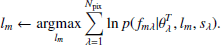
In Fig. 2 we compare the [Fe/H], α-enhancements, Teff, and log(g) of the common stars. The ARGOSα-enhancement is the average of the individual α-elements over iron ([α/Fe]). For APOGEE stars, ASPCAP provides individual α-elements with respect to iron ([Mg/Fe], [O/Fe], [Ca/Fe], ...) as well as an average of the α-elements to metallicity ([α/M]). For our comparisons, we chose the ASPCAP magnesium enhancement ([Mg/Fe]) because magnesium is produced only by supernova-II with no contribution from supernova-Ia. The bias and rms of each distribution are given in the upper left hand corner of each plot. The bias was calculated by subtracting the APOGEE values from the ARGOS values and taking the mean of the differences.
 |
Fig. 2. APOGEE-derived parameters (x axis) versus ARGOS derived parameters (y axis) for the 204 reference set stars observed by both surveys. The bias (mean of the differences) and rms of the distributions are given in the upper left hand corner of each plot. The reference set stars that are within one ARGOS observational error, 0.13 dex (0.1 dex), from the maximum [Fe/H] ([α/Fe]) value reached by the reference set are plotted as blue crosses (red triangles). |
The [Fe/H] comparison in the first plot of Fig. 2 shows that the surveys roughly agree between ∼ − 0.75 dex and ∼0 dex (limits in APOGEE [Fe/H]) with a scatter of ∼0.16 dex. However, beyond these limits, the deviation between the surveys increases, reaching up to ∼0.4 dex. The α-enhancement magnesium-enhancement comparison in the second plot shows that the ARGOS [α/Fe] estimates are on average ∼0.07 dex larger than the APOGEE [Mg/Fe] estimates. If we instead compare the ARGOS [α/Fe] estimates to the APOGEE [α/Fe] estimates, then the bias and rms of the distribution are larger at 0.12 dex and 0.15 dex, respectively. The Teff comparison in the third plot shows that the ARGOSTeff estimates are on average ∼300 K hotter than the APOGEETeff estimates. Finally, while there is a lot of scatter, the log(g) comparison in the last plot shows that the ARGOS log(g) values are generally higher than the APOGEE log(g) values.
The parameter comparisons show that for most of the common stars, the APOGEE and ARGOS parameters differ significantly. This could be due to a number of factors, such as observing in different wavelength regions (e.g. optical in ARGOS versus infrared in APOGEE), their use of different data analysis methods (e.g. photometric temperatures in ARGOS versus spectroscopic temperatures in APOGEE), or their use of different stellar models. In the following sections, we use the data-driven method, The Cannon, and this set of common stars to bring the APOGEE and ARGOS surveys on to the same parameter and abundance scales, thereby correcting the deviations we see in Fig. 2.
3. The Cannon method
The Cannon is a data-driven method that can cross-calibrate spectroscopic surveys. It has the advantage that it is very fast, requires no direct spectral model, and has measurement accuracy comparable to physics based methods even at lower S/N. The Cannon has been previously used to put different surveys on the same parameter and abundance scales using common stars (Casey et al. 2017; Ho et al. 2017; Birky et al. 2020; Galgano et al. 2020; Wheeler et al. 2020).
The Cannon uses a set of reference objects with known labels (i.e. Teff, log(g), [Fe/H], [X/Fe] ...), which describe the spectral variability well, to build a model to predict the spectrum from the labels. This model is then used to re-label the remaining stars in the survey. The word ‘label’ is a machine learning term that we use here to refer to stellar parameters and abundances together with one term. The set of common stars used to build the model is called the reference set.
The Cannon is built on two main assumptions: (i) stars with the same set of labels have the same spectra and (ii) spectra vary smoothly with changing labels.
Consider two surveys, A and B, where we want to put the stars in survey A onto the label scales of survey B using The Cannon. Assume we also have the required set of common stars between the two surveys to form the reference set. To cross calibrate the surveys, The Cannon performs two main steps: the training step and the application step. During the training step, the spectra from survey A and the labels from survey B of the reference set stars are used to train a generative model. Then, given a set of labels, this model predicts the probability density function for the flux at each wavelength. During the application step, the spectra of a new set of survey A stars (not the reference set) are re-labelled by the trained model. We call this set of stars the application set. If the region of the spectra fit to carries the label information and the reference set well represents the application set, then the new labels of survey A’s stars should be on survey B’s label scales. The success of the re-calibration can be quantified with a cross-validation procedure, the pick-on-out test described in Sect. 4.2, which returns the systematic uncertainty with which labels can be inferred from the data, as well as a comparison of the generated model spectra to the observational spectra for individual stars, using a χ2 metric.
In the next two subsections we describe the main steps of The Cannon in more detail.
3.1. The training step
During the training step, a generative model is trained such that it takes the labels as input and returns the flux at each wavelength of the spectrum. The functional form of the generative model, fnλ, can be written as a matrix equation:
 (1)
(1)
where θλ is a coefficient matrix, ln is a label matrix, and σ is the noise. The subscript n indicates the reference set star while subscript λ indicates the wavelength.
The coefficient matrix, θλ, contains the coefficients that control how much each label affects the flux at each pixel. The coefficients are calculated during the training step.
Here the label matrix, ln, is quadratic in the labels and for each star (each column in the matrix) has the form:
![Mathematical equation: $$ \begin{aligned} l_{n} \equiv [1,\, l_{(1\ldots n)},\, l_{(1\ldots n)} \cdot l_{(1\ldots n)}]. \end{aligned} $$](/articles/aa/full_html/2021/09/aa40990-21/aa40990-21-eq2.gif) (2)
(2)
If, for example, the generative model is trained on the labels Teff and log(g), then each column in the label matrix would be:
![Mathematical equation: $$ \begin{aligned} l_{n} \equiv [1,\, {T_{\rm eff}},\, \log (g),\, {T_{\rm eff}}\cdot {T_{\rm eff}},\, \log (g)\cdot \log (g),\, {T_{\rm eff}}\cdot \log (g)]. \end{aligned} $$](/articles/aa/full_html/2021/09/aa40990-21/aa40990-21-eq3.gif) (3)
(3)
The noise, σ, is the rms combination of the uncertainty in the flux at each wavelength due to observational errors, σnλ, and the intrinsic scatter at each wavelength in the model, sλ.
Equation (1) corresponds to the single-pixel log-likelihood function:
![Mathematical equation: $$ \begin{aligned} \ln p(f_{n\lambda } | \theta _{\lambda }^{T}, l_{n},s_{\lambda }) = -\frac{1}{2}\frac{[f_{n\lambda } - \theta _{\lambda }^{T} \cdot l_{n}]^{2}}{s_{\lambda }^{2} + \sigma _{n\lambda }^{2}} - \frac{1}{2}\ln (s_{\lambda }^{2} + \sigma _{n\lambda }^{2}). \end{aligned} $$](/articles/aa/full_html/2021/09/aa40990-21/aa40990-21-eq4.gif) (4)
(4)
During the training step, the coefficient matrix θλ and the model scatter sλ are determined by optimising the single-pixel log-likelihood in Eq. (4) for every pixel separately:
 (5)
(5)
During this step The Cannon uses the reference set stars to provide the label matrix, ln. The label matrix is held fixed while the coefficient matrix and model scatter are treated as free parameters.
3.2. The application step
In the training step, we have the label matrix, ln, and we solve for the coefficient matrix θλ and the scatter sλ. In the application step, we do the opposite: we have the coefficient matrix θλ and the scatter sλ and we solve for a new label matrix, lm. The subscript m is used in this step because the label matrix now corresponds to stars in the application set, not the reference set.
The label matrix, lm, is solved for by optimising the same log-likelihood function as Eq. (4). However, here this optimisation is performed using a non-linear least squares fit over the whole spectrum, instead of per pixel:
 (6)
(6)
4. A2A catalogue
In this paper we use The Cannon to put the stars from the ARGOS survey onto the APOGEE survey’s label scales for the following labels: [Fe/H], [Mg/Fe], Teff, log(g), and K-band extinction (Ak). After applying The Cannon to the ARGOS survey, we obtain a new catalogue containing the same stars observed by the ARGOS survey but with new label values. Other labels, such as line-of-sight velocity or apparent magnitude, remain unchanged. We call this new catalogue the A2A catalogue. In this section, we describe the reference and application sets used to build the A2A catalogue and perform three validation tests to confirm that the A2A catalogue is on the APOGEE scale. Lastly, we compare the A2A catalogue to the ARGOS catalogue and explain how we extracted the A2A RC and corresponding distances.
4.1. Reference and application sets
A reference set of stars, which is used to train The Cannon’s model, is composed of the stars that are observed by both surveys. The labels for this reference set come from the survey with the desired label scale (in our case APOGEE), while the spectra are taken from the other (in our case ARGOS). The model that is learned at training time should only be applied to stars that are well represented by the reference set. That is, applied to stars that span the label region of the training data, within which the model can interpolate but need not extrapolate. This can also be thought of as a selection in spectra. In our case, the 204 stars that are common to both the APOGEE and the ARGOS surveys (discussed in Sect. 2.3) formed the reference set for our Cannon model. The average S/N of the reference set is 46 for ARGOS and 107 for APOGEE.
These reference set stars are found in the following intervals in the ARGOS parameter space:
 (7a)
(7a)
 (7b)
(7b)
![Mathematical equation: $$ \begin{aligned}&-1.4 \le [\mathrm{Fe/H}]\,\,(\mathrm{dex})\le 0.18 , \end{aligned} $$](/articles/aa/full_html/2021/09/aa40990-21/aa40990-21-eq9.gif) (7c)
(7c)
![Mathematical equation: $$ \begin{aligned}&-0.062 \le [\alpha /\mathrm{Fe}]\,\,(\mathrm{dex}) \le 0.569. \end{aligned} $$](/articles/aa/full_html/2021/09/aa40990-21/aa40990-21-eq10.gif) (7d)
(7d)
We ignore the limits in Ak as this label was only included to stabilise the fits to the other labels. As such, we do not use the learned Ak label for science.
There are 20 435 ARGOS stars (∼79% of the ARGOS catalogue) within the 4D parameter space defined by intervals (7a)–(7d). These stars are considered to be well represented by the reference set and normally would have formed our application set. However, there are many stars with parameter values close to but just outside of the reference set limits. For example, if we extend all the limits by 1σARG, equal to the ARGOS observational error of each label, then we would include 2704 more stars in the application set (∼10.5% more of the ARGOS catalogue). Because these stars are still close to the reference set stars, the labels returned by The Cannon for these stars may be correct to the first order. To test whether we could extend any of the limits we used the following procedure: (i) Remove reference set stars 1σARG from each limit. This decreases the number of reference set stars. (ii) Train a new Cannon model on the reduced reference set. For clarity, we refer to this model as the minus-one-sigma (m1σ) model. (iii) Reprocess ARGOS spectra using the m1σ model to obtain new Cannon parameters for each star. The application set remains the same as the one processed by the original Cannon model. (iv) Compare the new Cannon labels from the m1σ model to the labels given by the original Cannon model.
For reference, the ARGOS observational errors, σARG, for [Fe/H], [α/Fe], Teff, and log(g) are: 0.13 dex, 0.1 dex, 100 K, and 0.3 dex, respectively.
We applied this test to each label limit separately and found that the extrapolation works best for the high [Fe/H] and high [α/Fe] limits. In Fig. 3, we compare the output labels produced by the original Cannon model against the output labels produced by the m1σ models trained on the reduced reference sets. The original Cannon model was trained on all 204 reference set stars, shown as the black, blue, and red markers in Fig. 2. The Fe-m1σ model (top plot) was trained on 149 reference set stars, shown as just the black and red markers in Fig. 2. The Mg-m1σ model (second plot) was trained on 199 reference set stars, shown as just the black and blue markers in Fig. 2. For each comparison (or plot) we only compare stars that have ARGOS parameter values in the 1σARG region we removed (regions occupied by the blue and red markers in Fig. 2). For both labels, fewer than 1% of stars have original Cannon model and m1σ model labels that differ by more than 1σARG.
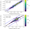 |
Fig. 3. Comparison of the [Fe/H] (top) and [Mg/Fe] (bottom) labels generated by the original Cannon model (x axis) and the m1σ models (y axis). In the top plot, only stars with ARGOS 0.05 < [Fe/H] (dex) < 0.18 are compared (the region in [Fe/H] spanned by the blue crosses in the top plot of Fig. 2). In the bottom plot, only stars with ARGOS 0.47 < [α/Fe] (dex) < 0.57 are compared (the region in [α/Fe] spanned by the red triangles in the plot second from the top in Fig. 2). The points are coloured by the point density. The black lines are one-to-one lines, and blue lines indicate ±1σARG. The bias and rms of each distribution are given in the top left corner of each plot. |
We also compared the labels produced by the original Cannon model to the labels produced by a Cannon model that was trained on a reference set that was simultaneously reduced by 1σARG in [Fe/H] and [Mg/Fe]. The reference set of this model consisted of only 144 stars, shown as the black markers in Fig. 2. We find that fewer than 1% of stars from this model have labels that differ from the original Cannon model by more than 1σARG in [Fe/H] and 2% in [Mg/Fe].
Because we found that we could accurately predict the [Fe/H] and [Mg/Fe] labels of stars in the 1σARG regions of the parameter space removed from the reference set, we made the assumption that we could apply the Cannon model trained on all 204 reference set stars to stars with ARGOS parameters 1σARG beyond the high [Fe/H] and [α/Fe] limits and still get approximately correct labels. Thus, we extended the limits of (7c) and (7d) to be:
![Mathematical equation: $$ \begin{aligned}&-1.4 \le [\mathrm{Fe/H}]\,\,(\mathrm{dex}) \le 0.31 ,\end{aligned} $$](/articles/aa/full_html/2021/09/aa40990-21/aa40990-21-eq11.gif) (8a)
(8a)
![Mathematical equation: $$ \begin{aligned}&-0.062 \le [\alpha /\mathrm{Fe}]\,\,(\mathrm{dex}) \le 0.669. \end{aligned} $$](/articles/aa/full_html/2021/09/aa40990-21/aa40990-21-eq12.gif) (8b)
(8b)
Limits (7a), (7b), (8a), and (8b) enabled us to process 85% of the ARGOS catalogue, or 21 577 stars. This increased the number of stars in the A2A catalogue with [Fe/H] above 0.5 dex by roughly 45%, the number of stars with [Fe/H] between 0 dex and 0.5 dex by roughly 23%, and the stars with [Fe/H] below −1 dex by roughly 10%.
In Sect. 5.1.2 we define our A2A catalogue used for the bulge analysis. This final catalogue has an additional colour cut applied (Eq. (12)), which removes an additional 252 stars, leaving 21 325 stars in the final catalogue. If the same colour cut is applied to the original ARGOS catalogue then the ARGOS catalogue would contain 23 487 stars. The final colour cut A2A catalogue is then 91% complete compared to the colour cut ARGOS catalogue. The parameter and abundance errors of the colour cut A2A catalogue are calculated in Sect. 4.2. For [Fe/H], [Mg/Fe], Teff, and log(g), the rms of the errors, σA2A, are 0.10 dex, 0.07 dex, 74 K, and 0.18 dex, respectively.
4.2. Validation tests
Given a reference set and an application set, The Cannon will always return new labels for the stars in the application set. However, if one is not careful, the returned labels can have large errors. In this section, we describe three validation tests we performed to verify that the labels returned by The Cannon are reasonable.
The first validation test we performed is a common machine learning test called the pick-one-out test. In this test, we created 204 models, each of which was trained on 203 stars from the reference set. The single star that was left out from the reference set changed between each model. Every model was then applied to the spectra of the respective left out star to obtain a new set of labels for it. How similar the new set of labels are to the original APOGEE labels indicates how well The Cannon can learn the APOGEE labels given the reference set. In Fig. 4 we compare the new Cannon labels of these stars to their APOGEE labels. For all four labels, the bias and rms, given in the upper left hand corner of each plot, are much lower than those from the ARGOS − APOGEE comparisons in Fig. 2. The strong agreement indicates that The Cannon can successfully learn the APOGEE labels from the ARGOS spectra using the reference set composed of the 204 common stars. The error on each parameter for each star in the A2A catalogue was calculated by adding in quadrature the rms value from the pick-one-out test and the small error that is output by the optimiser of The Cannon (see Sect. 3).
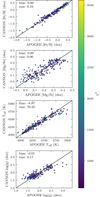 |
Fig. 4. Pick-one-out test. For each plot, each point represents a different reference set star. For a given point in a plot, the x axis value is the APOGEE-derived label and the y axis value is the label prediction from a Cannon model trained on all other (203) reference set stars. Therefore, for each point in each plot, the applied Cannon model is different than that of every other point. The points are coloured by their model χ2 values. The bias and rms of each distribution are given in the top left corner of each plot. |
As a second validation test we compared the model and observational spectra. The shape of the spectrum of a star can be affected by many different stellar parameters and abundances. Ideally, when training a model to describe a stellar spectrum with labels one would like to include all stellar labels that affect the spectrum’s shape. However, this would require a huge number of reference set stars, which we do not have. Instead, we made the approximation that the ARGOS spectra (8400 Å−8800 Å) could be well described by the five labels: [Fe/H], [Mg/Fe], Teff, log(g), and Ak. To test this, we compared the model spectra generated by The Cannon against the true observational spectra. This could be done because The Cannon trained model returns the flux at each pixel when given the labels (Eq. (1)). In Fig. 5 we plot the ARGOS spectra of a few example stars with a range of [Fe/H] values and cumulative χ2 values (sum of the pixel χ2 values) around the ARGOS pixel number (1697, see Fig. 6) versus their model spectra generated by The Cannon. For the model spectra, line thicknesses show the scatter of the fit by The Cannon at each wavelength. Figure 5 shows that the model spectra closely reproduce the true observational spectra. The overall good fit between the model spectra and the true spectra indicates that the spectra of the ARGOS stars can be well described by the variation in the five labels.
 |
Fig. 5. Normalised ARGOS spectra (black) versus the normalised model spectra (blue) generated by The Cannon for A2A stars with [Fe/H] values between −0.5 ≲ [Fe/H] ≲ 0.25. The plotted line thicknesses of the model spectra indicate the scatter of each fit by The Cannon. The residuals between the normalised ARGOS spectra and normalised model spectra are also shown in the panels below the spectra. |
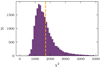 |
Fig. 6. Model χ2 distribution of A2A stars. The dashed orange line gives the number of pixels in each ARGOS spectrum. |
The third test we did was comparing the Teff − log(g) − [Fe/H] distribution of A2A stars to theoretical distributions. In the right hand plot of Fig. 7, we show the Teff − log(g) distribution of A2A stars coloured by mean [Fe/H] on top of 10 Gyr PARSEC isochrones with metallicities ranging from −2 dex to 0.6 dex (Tang et al. 2014; Chen et al. 2014, 2015; Bressan et al. 2012). The A2A stars tightly follow the PARSEC isochrones. Furthermore, even though no isochrone information was input into The Cannon, there are no A2A stars in non-physical regions of the diagram. The close fit of the A2A stars to the PARSEC isochrones supports that the label transfer was successful.
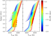 |
Fig. 7. Teff − log(g) distribution of ARGOS (left) and A2A (right) stars coloured by mean [Fe/H]. 10 Gyr PARSEC isochrones with −2 < [Fe/H] (dex) < 0.6 are plotted beneath. We note that the isochrones are plotted at 35% transparency in order to visually differentiate them from the 2D histograms. |
The success of these three tests shows that it is possible to train a Cannon model on a moderate number (204) of common stars and still obtain a set of labels with good precisions (see Sect. 4.1).
4.3. A2A versus ARGOS
In this section we compare the A2A catalogue to the ARGOS catalogue. In Fig. 7 we show the Teff − log(g) − [Fe/H] distributions of ARGOS stars (left) and A2A stars (right) on top of 10 Gyr PARSEC isochrones. The ARGOS stars very roughly follow the PARSEC isochrones. Many ARGOS stars also fall in non-physical regions of the parameter space. As discussed in the previous section, A2A stars have a much tighter alignment with the PARSEC isochrones with no stars falling in non-physical regions.
In Fig. 8 we show the ARGOS and A2A MDFs of all stars (top) and only RC stars (bottom). The most prominent difference between the MDFs of the surveys is that A2A obtains more very [Fe/H]-rich stars than ARGOS for all stars as well as when we restrict to only the RC. ARGOS has more solar to sub-solar stars until ∼ − 0.5 dex where A2A has more stars. Between ∼ − 1 and ∼ − 0.7 dex ARGOS has more stars for all stars and the RC. Below ∼ − 1 dex, the difference between ARGOS and A2A is small.
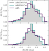 |
Fig. 8. Normalised ARGOS and A2A MDFs of all stars (top) and RC stars (bottom). The grey histogram includes stars from the full ARGOS catalogue, while the teal histogram includes only ARGOS stars that could be processed by The Cannon (same stars as in the A2A catalogue but with their old ARGOS labels). |
4.4. Red clump extraction and A2A distances
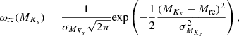
We statistically extracted RC stars from the A2A catalogue using the following probabilistic method: First, we determined the spectroscopic magnitudes, MKs, of each A2A star by fitting their log(g), Teff, and [Fe/H] parameters to theoretical isochrones. Then, using the spectroscopic magnitudes, we calculated a weight for each star that gives the probability that it is part of the RC. The functional form of this weight is a Gaussian:
 (9)
(9)
where Mrc = −1.61 ± 0.22 mag is the intrinsic magnitude of the RC (Alves 2000). We found that for 10 Gyr old PARSEC isochrones (Tang et al. 2014; Chen et al. 2014, 2015; Bressan et al. 2012) the spectroscopic magnitude varies with log(g) as dMKs/d(log g) = 2.33. The average A2A log(g) error is 0.18 dex, giving an average magnitude error of 0.42 mag. We added this in quadrature with the intrinsic width of the RC magnitude to obtain a total magnitude error of 0.47 mag for our RC sample. This is σMKs in Eq. (9). This magnitude-dependent weighing method extracts the RC from A2A by giving higher weights to stars that are likely to be part of the RC and lower weights to stars that are unlikely to be part of the RC.
To obtain distances for the A2A stars, we first treated each star as a RC star and assumed their absolute magnitudes were that of the RC (−1.61 mag). We then compared the RC absolute magnitude to the de-reddened apparent magnitude of each star, which we obtained using the Schlegel et al. (1998) extinction maps re-calibrated by Schlafly & Finkbeiner (2011). This method gave us the distance of each star assuming that it was a RC star. To account for the fact that not every A2A star is a RC star, we weighed the stars by how likely they were to be RC stars using the weight in Eq. (9). By weighing the stars in this manner, we treated all stars as RC stars but effectively removed the stars that were unlikely to be part of the RC by strongly de-weighting them.
The A2A catalogue contains 10 357 RC stars. We obtained this number by summing the RC weights (Eq. (9)).
5. Selection functions
The probability that any given star in the Galaxy is observed by a large survey programme is called the survey selection function (SSF); see Sharma et al. (2011) for a detailed discussion. In order to obtain unbiased parameter and abundance distributions of the Galactic bulge using the A2A and APOGEE surveys we must correct for their SSFs. Otherwise, it would not be clear if the distributions we obtain are the true distributions of the Galactic bulge, or whether they are biased by the selection choices of the surveys. In the next two sections, we discuss the A2A and APOGEE SSFs.
5.1. A2A selection function
The stars composing the A2A catalogue were selected from the ARGOS catalogue, which, in turn, was selected from a high quality (HQ) subset of the Two Micron All Sky Survey ( 2MASS; Skrutskie et al. 2006). In the following subsections we discuss the selection of the ARGOS survey from the HQ 2MASS subset and the selection of the A2A survey from the ARGOS survey.
5.1.1. Selection of ARGOS from HQ 2MASS
The ARGOS stars were selected from a HQ sub-sample of the 2MASS survey, requiring the stars to have high photometric quality flags (see Freeman et al. 2012), magnitudes between 11.5 ≤ Ks(mag)≤14.0, and colours (J − Ks)0 ≥ 0.38 mag. For each 2MASS star that met these requirements, its I0-band magnitude was estimated using the equation:
 (10)
(10)
Then, for each field, the ARGOS team randomly selected approximately 1000 stars roughly evenly distributed among the I0-band bins: 13−14 mag, 14−15 mag, and 15−16 mag. This was done in order to sample a roughly equal number of stars from the front, middle, and back regions of the bulge.
We used the following procedure to correct for the I0-band selection (similar to Portail et al. 2017a, their Sect. 5.1.1). First we took all 2MASS stars in a given field and applied the colour, magnitude, and quality cuts described above. Then, we estimated the I0-band magnitude of each remaining 2MASS star as well as of each ARGOS star using Eq. (10). We could then correct for the I0-band selection by weighing each ARGOS star by the ratio of the number of HQ 2MASS stars to the number of ARGOS stars in each I0-band bin and field:
 (11)
(11)
After the application of the weights in Eq. (11) to the ARGOS luminosity function (LF), we statistically recover the HQ 2MASS LF within the respective colour and magnitude limits. The upper plot of Fig. 9 shows this for the field (l, b) = (−10° , − 10° ).
 |
Fig. 9. Original and weighted Ks0-band LFs of ARGOS (top) and A2A (bottom) stars in the field (l, b) = (−10° , − 10° ). The HQ 2MASS LF is also plotted. The colour limits 0.45 ≤ (J − Ks)0 (mag)≤0.86 are applied to the LFs in the bottom plot. The A2A LF is slightly below the HQ 2MASS LF due to the parametric limits applied during the creation of the A2A catalogue. |
5.1.2. Selection of A2A from ARGOS
As the A2A stars were selected from the ARGOS catalogue, we also similarly corrected the A2A catalogue for the I0-band selection using the weights from Eq. (11). However, the weighted A2A LFs are systematically below the HQ 2MASS LFs because of the A2A selection from the ARGOS catalogue, which removed 4135 stars. These stars were removed because their spectra could not be processed by The Cannon (did not satisfy limits (7a), (7b), (8a), and (8b)). Because of this, we know the label values of these stars on the ARGOS scale but only have approximate knowledge of where they are on the APOGEE scale. To replicate this selection, we examined if the limits that removed these stars could be described using parameters that did not change during the label transfer.
The Teff limits (see (7a)) are simple to approximate as there is a near linear relationship between ARGOSTeff and colour, shown in Fig. 10. However, this substitution is not perfect and the colour limits must be chosen carefully as the Teff-colour distribution has some spread due to variations in the other labels. For example, stars with lower ARGOS [Fe/H] are hotter for constant colour (see the point colour in Fig. 10). If chosen incorrectly, the colour limits can remove many stars that satisfy limits (7a), (7b), (8a), and (8b). We found that the Teff limits are well approximated by the colour limits:
 (12)
(12)
 |
Fig. 10. ARGOSTeff versus de-reddened colour distribution of the full ARGOS catalogue. The point colour indicates the ARGOS [Fe/H]. The blue vertical lines show the reference set Teff limits (7a). The blue horizontal lines show the colour limits (12) used to approximate the Teff limits. |
We show in the lower plot of Fig. 9 the weighted A2A and HQ 2MASS LFs in the field (l, b) = (−10° , − 10° ); both of which have the colour cut in Eq. (12) applied. While the two LFs are close, there is still a slight deviation due to the other parametric limits.
Unfortunately, the other parametric limits are not as easily replaced using alternative parameters that remain constant during the label transfer. We take the final A2A catalogue to include all stars processed by The Cannon that: (i) have model χ2 values below 5000 (see Fig. 6), (ii) satisfy the limits (7a), (7b), (8a), and (8b), and (iii) are within the colour limits in Eq. (12).
Within these conditions, the A2A catalogue contains 21 325 stars. If we apply the colour cut (Eq. (12)) to the ARGOS catalogue then the ARGOS catalogue would contain 23 487 stars. Thus, the colour cut A2A catalogue is 91% complete compared to the colour cut ARGOS catalogue.
In the subsequent analysis of the bulge’s chemodynamical structure, we often select and plot A2A RC stars to obtain good distance estimates (see Sect. 4.4 for a discussion on RC extraction). We make the assumption that the reference set limits affect RC and red giant branch stars equally such that the A2A RC catalogue is also ∼91% complete. We test this assumption in Appendix A.
5.2. APOGEE selection function
The APOGEE sample we used for most of this work’s analysis is the HQSSF APOGEE bulge MSp. It is a sub-sample of the full APOGEE bulge MSp in that we also required the stars to have high quality ASPCAP parameters and abundances (see Sect. 2.2) and good SSF estimates. In this sample, only stars that are part of complete cohorts (i.e. groups of stars observed together during the same visits) have SSF estimates. Estimating the SSF for this sample proceeded in two steps. First, to account for the selection of the APOGEE bulge MSp from the HQ 2MASS subset, we used the publicly available python package APOGEE (Bovy et al. 2014; Bovy 2016; Mackereth & Bovy 2020). For each complete cohort, the program returned the ratio of the number of APOGEE MSp stars to the number of HQ 2MASS stars within the respective colour and magnitude limits of the cohort1. Then, we weighted each star in each cohort, ci, by the inverse of this ratio:
 (13)
(13)
Second, restricting our sample to APOGEE stars with HQ ASPCAP parameters and abundances (Sect. 2.2) removed ∼14% of the APOGEE bulge MSp. To correct for this selection we binned all APOGEE bulge MSp stars (including the stars with poor ASPCAP estimates) and all HQ ASPCAP MSp stars in magnitude, colour, and cohort. Then, we weighted each HQ ASPCAP MSp star by the ratio of the number of MSp stars to the number of HQ ASPCAP MSp stars in the colour and magnitude bin in which it fell:
 (14)
(14)
Figure 11 shows the result of the application of the weights in Eqs. (13) and (14) to the H-band LF of a cohort in the field (l, b) = (−2° ,0° ). We see that after the application of the weights, the LFs of the HQSSF APOGEE bulge MSp and HQ 2MASS subset approximately match.
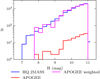 |
Fig. 11. Original and weighted APOGEEH-band LFs of the HQSSF bulge MSp for a cohort in the field (l, b) = (−2° ,0° ). The HQ 2MASS LF is also plotted. |
In Fig. 1, the red crosses indicate APOGEE field locations for which we could not use the APOGEE python package to obtain good SSF estimates of the observed stars. This occurred either because the cohorts composing the fields were not complete or because they did not contain any MSp stars. Removing these fields, as well as a few cohorts for which the weighted LF poorly reproduced the LF of its HQ 2MASS parent sample, leaves 23 512 stars in the HQSSF APOGEE bulge MSp.
In the subsequent analysis we restrict the HQSSF APOGEE bulge MSp further by requiring stars to have AstroNN distance errors of less than 20%. This roughly removes 5% of the HQSSF APOGEE bulge MSp leaving 22 340 APOGEE stars.
5.3. Selection of HQ 2MASS catalogues
So far we have described the A2A and APOGEE SSFs as well as the corresponding weights that were needed to statistically correct each survey to the magnitude and colour distributions of their respective HQ 2MASS parent samples. This is similar to the procedure done by Rojas-Arriagada et al. (2020), who used simple stellar populations to determine the fraction of giants with fixed distance modulus and metallicity that fall with in the APOGEE magnitude and colour ranges. Then using these fractions, they re-weighted the observed stars to the weights they had in the survey input sample. However, the input HQ 2MASS sample of each survey itself has a SSF relative to the real Galaxy (in practice, the current deepest photometric survey, VVV Minniti et al. 2010; Surot et al. 2019) due to photometric criteria, crowding, and extinction. The 2MASS SSF is strongest at low latitudes and is illustrated in Portail et al. (2017a, their Sect. 5.1.1). This SSF would be additionally required when comparing (or weighting by) the relative number densities of stars in different fields, especially those with different latitudes.
In this paper, we confine our analysis to small spatial bins, making use of RC distances for A2A and AstroNN distances for APOGEE. When we do this, the observed stars in a given bin are representative of the stellar population at that distance making further corrections of the HQ 2MASS survey magnitude distribution unnecessary. However, in practice, the bins we use have sizes ∼2 kpc, thus if there is a line-of-sight abundance gradient in a field, the fainter stars in a given bin could have a slightly different abundance distribution than the brighter stars as they trace somewhat larger distance. Figure 12 shows, for example bins, that no such effect is seen within the errors in either survey.
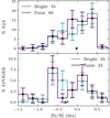 |
Fig. 12. MDFs of bright and faint stars in the same distance bins. Top: A2A RC stars from the field (l, b) = (0° , − 5° ) and the distance bin 6 to 8 kpc with the weights from Eq. (11) applied. Bottom: APOGEE stars from the field (l, b) = (0° , − 2° ) and the distance bin 6 to 8 kpc with the weights from Eqs. (13) and (14) applied. The number of stars in each MDF is given in the legend of each plot. The means of each histogram are given by the triangular markers. |
An additional effect could arise due to fields at different latitudes/heights contributing stars to the same distance bins. Specifically, lower latitude fields are generally more [Fe/H]-rich and have higher crowding than higher latitude fields due to the [Fe/H] and density gradients in the bulge. In such cases, by not correcting for the HQ 2MASS SSF we may introduce a slight bias against the lower latitude, higher [Fe/H] stars in each spatial bin. However, the effects of field mixing would be small in A2A as its fields are well separated and generally located at latitudes with low crowding (|b| ≥ 5°). Whereas for APOGEE, the effects of field mixing would also be small because at low latitudes (|b| < 4°), where the incompleteness of the HQ 2MASS catalogue is largest, the [Fe/H] gradient is nearly flat (Rich et al. 2012; Ness et al. 2016), and at high latitudes (|b| > 4°), where the [Fe/H] gradient is negative, the incompleteness of the HQ 2MASS catalogue is small. When we vary the width of our distance bins in |Z|, we do not find significant changes in the bulge [Fe/H] gradient. Therefore, we neglect field mixing effects in this paper.
5.4. Application of the SSF corrections
Here we illustrate the effect of the different spatial selections of the two surveys in the inner Galaxy, and then compare their SSF-corrected MDFs and [Mg/Fe] distribution functions (Mg-DFs) in regions of spatial overlap.
The first two plots in the top row of Fig. 13 show the APOGEE and A2A MDFs and Mg-DFs of all stars (RC for A2A) in each catalogue. APOGEE observes many stars near the Galactic plane and in the nearby disk that A2A misses, as illustrated in the right two plots of this row. These stars tend to be more [Fe/H]-rich and [Mg/Fe]-poor than stars at larger heights, causing much stronger [Fe/H]-rich and [Mg/Fe]-poor peaks in the APOGEE histograms than in A2A. In the second row of Fig. 13, the samples are restricted to smaller regions of overlap between the surveys, demanding |Z| ≥ 0.5 kpc and distances from the Sun between 4 and 12 kpc, and thereby removing many of the in-plane [Fe/H]-rich [Mg/Fe]-poor stars in the APOGEE catalogue. This causes the [Fe/H]-rich and [Mg/Fe]-poor peaks in the APOGEE MDF and Mg-DF to decrease, leading to better agreement with A2A. Some differences in the MDF and Mg-DF shapes are still expected, due to differences both in detailed coverage and in number density along the line-of-sight, as we did not correct each survey past the HQ 2MASS catalogues they were selected from.
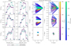 |
Fig. 13. SSF-corrected MDFs (first column), Mg-DFs (second column), and their respective positional information (third and fourth columns) of A2A and APOGEE stars with [Fe/H] > −1 dex. The top row includes all stars in each catalogue, while the stars in the second and third rows are restricted to successively smaller areas. The A2A stars are restricted to RC stars. The mean [Fe/H] and [Mg/Fe] values of each MDF and Mg-DF are shown by the triangular markers in each plot. |
However, if we restrict the sample to a smaller distance bin as shown in the third row of Fig. 13, such effects are significantly weakened. Now the MDFs and Mg-DFs agree within the errors except for the most [Fe/H]-poor bin in the MDF and the most [Mg/Fe]-rich bin (> 0.35 dex) in the Mg-DF where APOGEE observes a larger fraction of stars.
5.5. The high [Mg/Fe] and low [Fe/H] stars
In the following sections we see that the discrepancy seen in Fig. 13 at the high [Mg/Fe] end is widespread in the bulge occurring in both the inner and outer bulge and at various heights from the plane, even after the SSF corrections are applied. We believe that this discrepancy can be at least partially explained by the limited Teff range spanned by the reference set (see Fig. B.2) coupled with systematic trends between the ASPCAP Teff and abundances of the APOGEE stars (Jönsson et al. 2018; Jofré et al. 2019). Figure B.1 shows the trends between ASPCAP Teff and [Mg/Fe] in the APOGEE bulge sample for a range of [Fe/H] bins and roughly fixed stellar distance, height from the plane, and S/N. From this figure, we can see that regardless of [Fe/H], the average [Mg/Fe] of the APOGEE stars generally increases with increasing Teff until ∼4000 K, after which it decreases with increasing Teff. The Teff range of the reference set, shown by the blue shaded region in Fig. B.1, does not reach below ∼4000 K. Because of this, The Cannon cannot learn the trends between Teff and the abundances in ASPCAP that exist below ∼4000 K. Furthermore, this Teff cut means that the A2A catalogue would not contain many of these [Mg/Fe]-rich stars with Teff values just below ∼4000 K. Together, this could explain why the APOGEE and A2A Mg-DFs disagree at the high [Mg/Fe] end. As we will see in Sect. 6.4, [Mg/Fe]-rich stars are typically also [Fe/H]-poor. This could then explain why A2A also observes fewer [Fe/H]-poor stars as compared to APOGEE.
We cannot currently be sure whether the trends we observe between ASPCAP Teff and [Mg/Fe] are physical or systematic and therefore whether the lack of these trends in A2A is problematic or not.
6. Abundance structure of the bulge
We now present how the abundances and kinematics vary over the Galactic bulge using the combined APOGEE and A2A catalogues.
For all figures in this section, we restrict the A2A stars to RC stars and require the APOGEE stars to have AstroNN distance errors less than 20%. Unless mentioned otherwise, we use the HQSSF APOGEE bulge MSp and, correct each survey to the HQ 2MASS catalogue they were selected from, and limit stars to [Fe/H] > −1 dex. Furthermore, when combining stars from different spatial bins, we weight the stars in each distance bin to correct for the SSF effects on the abundance distributions but then in each bin we re-weight both surveys such that the sum of their weights is equal to the number of stars (RC for A2A) contributed by each survey.
6.1. Mean abundance maps
We first examine the overall variation in [Fe/H] and [Mg/Fe] with position in the Galactic bulge. Figure 14 shows the mean [Fe/H] and [Mg/Fe] values in each field of stars with distances from the Sun between 4 and 12 kpc. The APOGEE and A2A surveys generally agree on the overall [Fe/H] and [Mg/Fe] trends with Galactic longitude and latitude. As expected, the high latitude fields are more [Fe/H]-poor and [Mg/Fe]-rich than the low latitude fields. Additionally, at low latitudes, the stars are more [Fe/H]-poor and [Mg/Fe]-rich near the GC than they are in the long bar and disk. Because of this, the vertical abundance gradients at large absolute longitudes are steeper near the plane than at small absolute longitudes. Similar abundance trends with Galactic longitude and latitude were seen by Ness et al. (2016) using APOGEE DR12 data.
 |
Fig. 14. SSF-corrected mean [Fe/H] (left) and [Mg/Fe] (right) in APOGEE (circles) and A2A (squares) fields for stars with [Fe/H] > −1 dex and distances from the Sun between 4 and 12 kpc. |
Figure 15 shows illustrative mean X − Z and X − Y [Fe/H] maps built using A2A and APOGEE stars separately and combined. Here we use a Galactocentric left-handed coordinate system with positive X directed towards the Sun, Y along positive longitude (l), and Z along positive latitude (b). The assumed value of the solar distance is R0 = 8.2 kpc (Bland-Hawthorn & Gerhard 2016). In order to show all our data, we do not restrict the third dimension in each plot. From the X − Z plots in the top row, we see that the stars from both surveys become more [Fe/H]-rich towards the plane. Additionally, both the individual and combined maps show that the more [Fe/H]-rich stars dominate at larger |Z| at small |X| than they do at larger |X|. Lastly, the stars at the GC are more [Fe/H]-poor than their immediate surroundings.
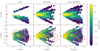 |
Fig. 15. SSF-corrected mean [Fe/H] distributions in the X − Z plane (top row) and X − Y plane (bottom row) of A2A (left column), APOGEE (middle column), and combined (right column) stars with [Fe/H] > −1 dex. The red lines trace the density distribution of the Milky Way’s bar obtained from a Portail et al. (2017a) bulge-bar model. The red star in each plot marks the position of the Sun. |
In the bottom row of Fig. 15, on top of the X − Y [Fe/H] maps, we plot the bulge’s density distribution obtained from one of the Portail et al. (2017a) bulge-bar models. These models were fit to the RC density of VVV, UKIDSS, and 2MASS and to the stellar kinematics of BRAVA, OGLE, and ARGOS. The model we use has a pattern speed of Ωb = 37.5 km s−1 kpc−1 as that was found to give the best visual match to the VIRAC proper motion data (Clarke et al. 2019). In both the separate and combined X − Y maps, the near side of the bulge appears to be more [Fe/H]-rich than the far side. This is an effect of the field viewing angles, which cause the nearer stars to be preferentially sampled closer to the plane than the farther stars.
Because we do not restrict the surveys to small bins in the projection direction in Fig. 15, the relative weighting by number density is incorrect, especially at low heights in the face-on view (see Sect. 5). In the following plots of this section, we restrict the abundance maps to smaller bins in vertical height and distance in order to minimise this effect.
The bar causes an asymmetry in the spatial maps. To remove this asymmetry, we reorient the following plots to the bar reference system taking the bar angle to be 25° (Bovy et al. 2019). The coordinate system is: the bar long axis (Xbar), the bar short axis (Ybar), and the height from the Galactic plane (Z). For these figures we also symmetrise the distribution of stars in order to fill in gaps in our spatial coverage as well as increase the statistics. The symmetrisation is done by reflecting each star into each projected quadrant.
The top row of Fig. 16 shows the symmetrised mean [Fe/H] maps in the |Xbar|−|Z| plane for different slices in |Ybar| using stars from both APOGEE and A2A. On top of the map, we plot the bulge density distribution (white dotted lines) obtained from the Portail et al. (2017a) model. In all |Ybar| slices, the mean [Fe/H] generally increases towards the plane. However, for |Ybar| < 1 kpc and |Xbar| < 1 kpc, the mean [Fe/H] increases rapidly towards the plane, then remains roughly constant between 0.3 ≲ |Z| (kpc) ≲ 0.7, and finally decreases within the inner few 100 pc. This is not the case well outside the boxy-peanut (b/p) bulge lobes (|Xbar| > 3 kpc) where, within 1 kpc from the Galactic plane, the mean [Fe/H] values increase rapidly towards the plane with no large regions of constant mean [Fe/H] or inversions of the [Fe/H] gradient. Furthermore, the [Fe/H] structure in the |Ybar| < 1 kpc slice (top left panel of Fig. 16) is puffed up and X-shaped with the more [Fe/H]-rich stars dominating at large |Z| inside the b/p bulge lobes (|Xbar|∼2 kpc). The X-shape is seen in mean [Fe/H] values between 0 dex and −0.4 dex. For |Ybar| > 1 kpc, the mean [Fe/H] structure becomes increasingly flat with increasing |Ybar| and the difference between large and small |Xbar| decreases. In the 1 ≤ |Ybar| (kpc) < 2 slice (middle panel of Fig. 16), one still sees a slight pinching/X-shape in the [Fe/H] distribution at mean [Fe/H] values of ∼ − 0.25 dex.
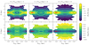 |
Fig. 16. SSF-corrected symmetrised mean [Fe/H] (top row) and [Mg/Fe] (bottom row) distribution in the Xbar − Z plane for combined A2A and APOGEE stars with [Fe/H] > −1 dex in slices of |Ybar|. The dotted white lines trace the density distribution obtained from a Portail et al. (2017a) bulge-bar model. The red arrow points in the direction of the Sun. |
The bottom row of Fig. 16 shows the symmetrised mean [Mg/Fe] distribution for APOGEE and A2A stars in the |Xbar|−|Z| plane in slices of |Ybar|. The [Mg/Fe] maps mirror the [Fe/H] maps. The mean [Mg/Fe] generally decreases towards the plane in all |Ybar| slices. For |Ybar| < 1 kpc (bottom left panel of Fig. 16) and |Xbar| < 1 kpc, the rate of decrease of the mean [Mg/Fe] is slower and the gradient inverts at small |Z| such that the inner bulge is slightly more [Mg/Fe]-rich than its immediate surroundings. A clear X-shape is seen in the mean [Mg/Fe] distribution at roughly [Mg/Fe] ≈ 0.175 dex in the |Ybar| < 1 kpc slice. In the region of the X-shape, the [Mg/Fe]-poor stars dominate at larger |Z| than they do at larger |Xbar| or larger |Ybar|. For larger |Ybar|, the mean [Mg/Fe] distribution becomes increasingly flat.
The [Fe/H] and [Mg/Fe] distributions are more strongly pinched than the density distribution in the |Ybar| < 1 kpc slice (left panels of Fig. 16). At larger |Ybar|, the density contours and the [Fe/H] and [Mg/Fe] contours are in better agreement.
Figure 17 shows the symmetrised mean [Fe/H] maps in the |Xbar|−|Ybar| plane for different slices in |Z|. The stars are restricted to the bar region, which we approximate as an ellipse with a semi-major axis and axis ratio of 5 kpc and 0.4, respectively (see Fig. 15). For |Z| < 0.3 kpc, the centre of the bar is more [Fe/H]-poor than the bar ends. As the distance from the plane increases, this reverses at ∼0.75 kpc. At greater heights, we again see that the centre of the bar is more [Fe/H]-poor than the bar ends.
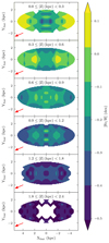 |
Fig. 17. SSF-corrected symmetrised mean [Fe/H] distribution in vertical slices along the Galactic bar for combined A2A and APOGEE stars with [Fe/H] > −1 dex. The red arrow points in the direction of the Sun. |
In near infrared star counts, the Galactic bar has a half length of ∼5 kpc (Wegg et al. 2015). The b/p bulge extends out to ∼2 kpc from the GC. The bar region that extends outside the b/p bulge is known as the long bar. Wegg et al. (2015) shows that the long bar is composed of two bar components, the thin bar with a scale height of 180 pc, extending to ∼4.6 kpc, and the super thin bar with a scale height of 45 pc, reaching ∼5 kpc. We do not have the resolution to detect an [Fe/H] or a [Mg/Fe] signature of the super thin bar; however, the top panel of Fig. 17 extents to roughly 1.7 thin bar scale heights above the plane. From this, we can approximately say that the combined long bar is super solar in [Fe/H] (also seen in the top left panel of Fig. 16). The lower left panel of Fig. 16 also shows that the region occupied by the long bar is nearly solar in [Mg/Fe]. This is in contrast to the inner region of the b/p bulge, which has a mean sub-solar [Fe/H] value and is more [Mg/Fe]-rich.
6.2. Abundance gradients
Having shown how [Fe/H] and [Mg/Fe] vary over the bulge, we now quantify the vertical and horizontal abundance gradients in the various bulge regions. In Fig. 18, we present the mean [Fe/H] and [Mg/Fe] profiles for A2A and APOGEE stars in the inner bulge (left column) and long bar-outer bulge region (right column) as a function of |Z|. We take the inner bulge to be the region within |Xbar| < 2 kpc and |Ybar| < 1 kpc and the long bar-outer bulge region to be the region within 2.5 ≤ |Xbar| (kpc) < 4.5 kpc and |Ybar| < 1 kpc.
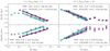 |
Fig. 18. SSF-corrected mean [Fe/H] (top row) and [Mg/Fe] (bottom row) vertical abundance profiles for A2A and APOGEE stars in the inner b/p bulge (|Xbar| < 2 kpc, |Ybar| < 1 kpc; left) and long bar-outer bulge regions (2.5 kpc | ≤ Xbar| < 4.5 kpc, |Ybar| < 1 kpc; right). The A2A and APOGEE gradients of the regions shown by the teal and purple lines are given in the legend of each diagram; error ranges of the linear fits are shown by the shaded regions. For all plots, we require the stars to have [Fe/H] > −1 dex. |
The APOGEE and A2A [Fe/H] and [Mg/Fe] gradients agree within the errors in both regions of the bulge. However, the [Fe/H] and [Mg/Fe] profiles in the inner bulge are offset by roughly 0.1 dex and 0.05 dex, respectively. These offsets are at least partially due to missing [Fe/H]-poor, [Mg/Fe]-rich stars in A2A as discussed in Sect. 5.5.
The inner bulge has a different vertical [Fe/H] profile than the long bar-outer bulge region. For 0.7 ≲ |Z| (kpc) ≲ 2, the inner bulge [Fe/H] gradient is ∼ − 0.41 dex kpc−1; at lower heights, between 0.3 ≲ |Z| (kpc) ≲ 0.7 it flattens at [Fe/H] ≈ −0.12 dex. This flattening of the [Fe/H] gradient is only clear in the APOGEE data (the A2A coverage is too sparse in this area), but was previously seen also by Rich et al. (2012, 2007) and Ness et al. (2016). Below 0.3 kpc the mean [Fe/H] slightly decreases. This inversion of the mean [Fe/H] gradient was also seen in Fig. 16.
The [Fe/H] gradient of the long bar-outer bulge region is roughly flat between 1.25 ≲ |Z| (kpc) ≲ 2.25 at a value of ∼ − 0.44 dex. For |Z| ≲ 1.25 kpc, the gradient is ∼ − 0.44 dex kpc−1 and has no inner flattening.
Using stars with |l| < 11°, Rojas-Arriagada et al. (2020) finds the bulge vertical metallicity gradient to be −0.09 dex kpc−1 for |Z| < 0.7 kpc and −0.44 dex kpc−1 for 0.7 < |Z| (kpc) < 1.2. Beyond |Z| > 1.2 kpc, Rojas-Arriagada et al. (2020) finds a noisy but flat profile. Assuming the bar is at an angle of 25° with respect to the Sun, the 11° limit in Galactic longitude restricts their sample to ≲2.7 kpc along the bar, or roughly the region we refer to as the inner bulge. Thus, their vertical metallicity gradient is consistent with our inner bulge vertical metallicity gradient. However, our increased Galactic longitude range allows us to see that the flattening at small |Z| only occurs in the inner bulge and not in the long bar-outer bulge region.
The [Mg/Fe] profiles mirror the [Fe/H] profiles. For the inner bulge, the [Mg/Fe] profile is roughly flat for |Z| ≲ 0.7 kpc at [Mg/Fe] ≈ 0.19 dex. For |Z| ≳ 0.7 kpc, the [Mg/Fe] gradient is ∼0.11 dex kpc−1. In the long bar-outer bulge region, the [Mg/Fe] gradient is ∼0.17 dex kpc−1 in APOGEE and ∼0.13 dex kpc−1 in A2A between 0 ≲ |Z| (kpc) ≲ 1.25. For |Z| ≳ 1.25 kpc the [Mg/Fe] profile flattens at ∼0.27 dex.
The top row of Fig. 19 shows the horizontal mean [Fe/H] profile of A2A and APOGEE stars along the Galactic bar at different heights above the plane. For |Z| ≲ 0.3 kpc, the radial [Fe/H] gradient is steep and positive. However, the stars at |Xbar| ≳ 2 − 3 kpc from both surveys strongly decrease in [Fe/H] with increasing height from the plane. For stars at |Xbar|≲2 − 3 kpc this effect is less pronounced. For A2A, this decrease in mean [Fe/H] within |Xbar| ≲ 2 − 3 kpc is stronger at smaller |Xbar|. This reflects the transitions between the relatively [Fe/H]-poor central bulge, the [Fe/H]-rich long bar near the Galactic plane, the region of enhanced [Fe/H] in the b/p bulge, and the [Fe/H]-poor region above the long bar in Fig. 16.
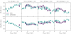 |
Fig. 19. SSF-corrected mean [Fe/H] (top row) and [Mg/Fe] (bottom row) horizontal abundance profiles of A2A and APOGEE stars along the bar and at different heights above the Galactic plane. For all plots, we require the stars to have [Fe/H] > −1 dex and |Ybar| < 1 kpc. |
The [Mg/Fe] horizontal profiles of both surveys are shown in the bottom row of Fig. 19. For |Z| ≲ 0.3 kpc, the mean radial [Mg/Fe] gradient is steep and negative. However, as the distance from the plane increases the stars at large |Xbar| increase in [Mg/Fe], causing the profile to flatten. At large |Z|, a minimum in [Mg/Fe] is seen around |Xbar|≈2 kpc. This profile is due to the lobes of the b/p bulge.
As was the case for the vertical gradients, there are clear offsets between the APOGEE and A2A horizontal profiles in [Fe/H] and [Mg/Fe], especially for |Xbar| < 2 kpc. This could at least in part be due to the limited Teff range of the reference set (see Sect. 5.5).
6.3. Shape of bulge abundance distribution functions
So far we have only examined how the mean [Fe/H] and [Mg/Fe] vary with position in the bulge. In this section, we illustrate how the MDFs and Mg-DFs change with position in the bulge.
In Fig. 20 we plot the generalised MDFs and Mg-DFs of A2A (RC) and APOGEE stars in the inner bulge for 0 < |Z| (kpc) < 1.8 in bins of width 0.3 kpc. The bins are chosen such that they each contain at least 100 distinct stars. The Gaussian smoothing of each stars is 0.1 dex in the MDFs and 0.033 dex in the Mg-DFs. We see that, while there are some deviations, both surveys show similar trends in their MDFs with |Z|. Far from the plane, the MDFs of both surveys are dominated by a strong peak at ∼ − 0.4 to ∼ − 0.5 dex. As the distance from the plane decreases, a solar and super solar peak in [Fe/H] grow and become prominent. The surveys show a stronger difference in their Mg-DFs. In APOGEE, far from the plane the Mg-DF is dominated by a single peak at ∼0.3 dex. As the distance from the plane decreases, a second peak at ∼0.05 dex increases in strength, such that near the Galactic plane, the two peaks are nearly equal in strength. In A2A, the Mg-DF far from the plane is also dominated by a single peak at ∼0.3 dex. However, as the distance from the plane decreases, the strength of the high [Mg/Fe] peak decreases and the stars below ∼0.25 dex increase in strength. The peak at ∼0.3 dex, seen in the APOGEE Mg-DF, is not prominent in the A2A Mg-DFs near the plane.
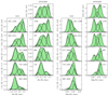 |
Fig. 20. Generalised MDFs (left two columns) and Mg-DFs (right two columns) of A2A (RC) and APOGEE stars at different absolute heights above the plane in the inner bulge, shown as filled distributions in green. The stars are required to have |Xbar| < 2 kpc, |Ybar| < 1 kpc, and [Fe/H] > −1 dex. Gaussian mixture decompositions at each height are also shown, in black (individual Gaussians and sums). The number of distinct stars composing each distribution is given in each plot. The number in brackets in the A2A plots gives the number (total weight) of A2A RC stars. |
Using the affine-invariant Markov chain Monte Carlo sampler emcee (Foreman-Mackey et al. 2013), we fit a four-component Gaussian mixture model (GMM) to each generalised MDF and a three-component GMM to each generalised Mg-DF. The Gaussians and their sums are plotted on top of the generalised MDFs and Mg-DFs in Fig. 20. To see the variation in the MDF and the Mg-DF Gaussian parameters clearly, we plot the Gaussian means, sigmas, and weights against |Z| in Fig. 21. To minimise the effects of noise, we only connect points in Fig. 21 with at least 300 distinct stars.
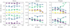 |
Fig. 21. Variation in the Gaussian parameters with height from the Galactic plane (|Z|) for the inner bulge. Top row: parameters from the MDF decompositions. Bottom row: parameters from the Mg-DF decompositions. The lines connect points with at least 300 distinct stars. Triangular markers and solid lines show the A2A decompositions. Circular markers and dashed lines show the APOGEE decompositions. |
The top left plot of Fig. 21 shows the variation in the MDF Gaussian means with |Z|. Both the A2A and APOGEE MDFs are well fit by a super solar [Fe/H] Gaussian (A), an intermediate [Fe/H] Gaussian (B), an [Fe/H]-poor Gaussian (C), and a very [Fe/H]-poor Gaussian (D). The overall variation in the [Fe/H] means with latitude is not substantial. The top middle plot shows the MDF sigma variations with |Z|. Gaussian B generally has the largest sigma closely followed by C, and then A and D, which are nearly equal in sigma. The top right plot shows the MDF weight variations with |Z|. The weights of all Gaussians are roughly constant below |Z|≈0.7 kpc, with B having marginally the largest weight. For |Z| ≳ 0.7 kpc, the most significant metal-poor Gaussian C increases, while the other two decrease such that C becomes the most dominant at large |Z|. Gaussian D is the weakest component at all heights as it never reaches over 10% in weight.
The variation in the Gaussian parameters from the three Gaussians fit to the Mg-DFs in the inner bulge is shown in the bottom row of Fig. 21. The bottom left plot shows the variation in the Gaussian means with |Z|. The Mg-DFs of both surveys are well fit by a [Mg/Fe]-normal Gaussian (Â), an intermediate [Mg/Fe] Gaussian ( ), and a [Mg/Fe]-rich Gaussian (Ĉ). The bottom middle plot shows the sigma variation in the Gaussians with |Z|. The A2A Gaussian
  generally has the highest sigma by ∼0.025 dex. The rest of the Gaussians have nearly equal sigma values. The bottom left plot shows the variations in the weights with |Z|. The Gaussian weights are constant below ∼0.7 kpc and nearly equal in weight. Above ∼0.7 kpc, the weight of Gaussian  decreases with increasing |Z| such that at ∼1.7 kpc its weight is nearly zero. Above ∼0.7 kpc, the behaviours of Gaussians
  and Ĉ strongly differ between the A2A and APOGEE surveys. As |Z| increases, the APOGEE weights of Gaussians Ĉ and
  increase and remain roughly constant, respectively, while the A2A weights of Gaussians Ĉ and
  remain constant and increase, respectively.
In Fig. 22 we perform a similar procedure as in Fig. 20 but on the long bar-outer bulge region. Using both surveys, we obtain generalised MDFs and Mg-DFs with smoothings of ∼0.1 dex and ∼0.033 dex, respectively, and their Gaussian decompositions in |Z| bins of width 0.3 kpc between 0 < |Z| (kpc) < 2.1. As was the case with the inner bulge, the more [Fe/H]-poor [Mg/Fe]-rich stars dominate far from the plane while the more [Fe/H]-rich [Mg/Fe]-poor stars dominate close to the plane.
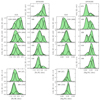 |
Fig. 22. Same as Fig. 20 except for the long bar-outer bulge region. The stars are required to have 2.5 kpc ≤ |Xbar| < 4.5 kpc, |Ybar| < 1 kpc, and [Fe/H] > −1 dex. |
The variations in the MDF Gaussian parameters with |Z| are shown in the top row of Fig. 23. We only connect points with at least 300 distinct stars to minimise noise. Similarly to the inner bulge, the top left plot shows that the long bar-outer bulge region is well fit by a super solar [Fe/H] Gaussian (A), an intermediate [Fe/H] Gaussian (B), an [Fe/H]-poor Gaussian (C), and a very [Fe/H]-poor Gaussian (D). The sigma variations are shown in the top middle plot. Gaussian B has the largest sigma value, sequentially followed by Gaussians C, A and D. The variations of the MDF Gaussian weights are shown in the top right plot. At |Z| ≳ 1 kpc, the weights of the Gaussians are similar to those of the inner bulge, with C dominating over B and A. At low |Z| the weight of the most metal-rich Gaussian A is higher than weight of C, the most significant metal-poor Gaussian. The transition in weight occurs at lower |Z| than in the inner bulge. Furthermore, for |Z| ≲ 0.7 kpc, the weight profiles of A and C are not constant, but continue to increase and decrease towards the Galactic plane, respectively. This is consistent with the profiles in Fig. 18. The weight of Gaussian D is weak at all heights, never rising above 10%.
In the bottom row of Fig. 23 we plot the variation of the Mg-DFs Gaussian parameters. The left most plot shows the variation in the Gaussian means. The Mg-DFs of both surveys are well fit by a [Mg/Fe]-normal Gaussian (Â), an intermediate [Mg/Fe] Gaussian ( ), and a [Mg/Fe]-rich Gaussian (Ĉ). We see a significant offset between the Gaussian
  means from both surveys. Furthermore, at |Z|≈1 kpc the Gaussians  means have a large offset. The bottom right plot shows the Gaussian weight variations with |Z|. For both surveys, the [Mg/Fe]-rich Gaussian Ĉ is strong at high |Z| and decreases in weight with decreasing |Z|, while the [Mg/Fe]-normal Gaussian  is very weak at high |Z| and increases in weight with decreasing |Z|. Because of these trends, close to the plane, Gaussian  dominates and Gaussian Ĉ is near zero in weight. At most heights, the Gaussian
  weight behaviour from both surveys deviates with the weight of Gaussian
  from A2A being much larger than the weight of Gaussian
  from APOGEE. Accordingly, the weight of Gaussian Ĉ from A2A is lower than the weight of the correspondingly [Mg/Fe]-rich Gaussian Ĉ from APOGEE at most heights.
By comparing the APOGEE weight behaviour of the MDF and Mg-DF Gaussians in both regions of the bulge, it is clear that Gaussians A, B, and C from the MDF decomposition roughly correspond to Gaussians Â,  , and Ĉ from the Mg-DF decomposition. However, in the outer bulge, Gaussian  is higher in weight than Gaussian A, while Gaussian B is higher in weight than Gaussian
  . Therefore, there is mixing between the Gaussians with some stars that compose Gaussians A and B in APOGEE being part of Gaussians
  and Â, respectively. For A2A, Gaussian A corresponds to Gaussian Â. However, the behaviours of Gaussians B and C from A2A from the MDF decomposition differ strongly from the behaviours of Gaussians
  and Ĉ from the Mg-DF decomposition. This deviation in Gaussian weight behaviour is much stronger in the inner bulge than in the outer bulge.
Overall, it appears that the A2A stars do not reach as high in [Mg/Fe] as the APOGEE stars do. Because of this, the APOGEE and A2A Mg-DFs deviate in shape at the [Mg/Fe]-rich end. We suspect that this may be due to the limited Teff range of the reference set used to train The Cannon model for the A2A catalogue (see Sect. 5.5 for a more detailed discussion on this).
Multiple other surveys (Rojas-Arriagada et al. 2017; Zoccali et al. 2017; Hill et al. 2011; Schultheis et al. 2017; Uttenthaler et al. 2012) report the bulge MDF to be bi-modal. The [Fe/H]-rich Gaussians in many of these surveys have a mean value of ∼0.3 dex, similar to the mean of our most [Fe/H]-rich Gaussian in both the inner and outer bulge. Recently, Rojas-Arriagada et al. (2020) analysed the bulge MDF using a larger sample from APOGEE DR16 data and reported that the bulge is best represented by the superposition of three Gaussian components with nearly constant means at 0.32 dex, −0.17 dex, and −0.66 dex. While we find that the bulge is best fit by four Gaussians, the fourth most [Fe/H]-poor Gaussian is not very significant and we mainly include it to improve the fit. In the inner bulge, the mean values of Gaussian A are similar to that of the most [Fe/H]-rich Gaussian of Rojas-Arriagada et al. (2020). However, in the inner bulge the means of Gaussians B and C are generally more [Fe/H]-rich than their two most [Fe/H]-poor Gaussians. This is likely due to the inclusion of the fourth [Fe/H]-poor Gaussian. Alternatively, the difference may arise from differing SSF-correcting methods or differing distance criteria. Thus, we do not believe that our results significantly differ from those of Rojas-Arriagada et al. (2020).
6.4. [Mg/Fe]–[Fe/H] distribution
In this section we present how the [Mg/Fe] − [Fe/H] distribution changes along the Galactic bar using a similar method to Hayden et al. (2015) and Queiroz et al. (2020b).
In Fig. 24, using stars from both the A2A and APOGEE, we plot the [Mg/Fe] − [Fe/H] distribution along the bar in bins of |Z| and |Xbar|, requiring |Ybar| < 1 kpc. We colour the points by the Gaussian kernel-density estimation using band-widths that obey Scott’s rule (Scott 1992).
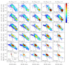 |
Fig. 24. [Mg/Fe] − [Fe/H] distribution of A2A and APOGEE stars in intervals of height from the plane (|Z|, kpc) and distance along the bar (|Xbar|, kpc). The stars are required to have |Ybar| < 1 kpc. The point colour gives the Gaussian kernel density estimate. The dashed lines separate the different regions in the parameter space generally populated by the halo, thin disk, and thick disk (defined in the lower-leftmost plot; see text). The number of stars composing each plot (A2A RC stars + APOGEE stars) is given in the lower left corner of each plot. |
Figure 24 shows that the [Mg/Fe] − [Fe/H] distribution of the bulge and bar has two main maxima, an ‘[Fe/H] rich-[Mg/Fe] poor’ maximum and an ‘[Fe/H] poor-[Mg/Fe] rich’ maximum. These maxima vary in strength with position along the bar. The ‘[Fe/H] poor-[Mg/Fe] rich’ stars dominate away from the plane while the ‘[Fe/H] rich-[Mg/Fe] poor’ stars dominate close to the plane. This trend is weaker at smaller |Xbar|.
Hayden et al. (2015) concluded using data from APOGEE DR12 (Alam et al. 2015) that the [α/Fe] − [Fe/H] distribution of the outer bulge appeared to be a single sequence with ‘high [α/Fe]-low [Fe/H]’ stars dominating far from the plane and ‘low [α/Fe]-high [Fe/H]’ stars dominating close to the plane. Conversely, Rojas-Arriagada et al. (2019) concluded using data from APOGEE DR14 that the inner bulge [Mg/Fe] − [Fe/H] distribution was composed of two sequences, a ‘high [Mg/Fe]-low [Fe/H]’ sequence and a ‘low [Mg/Fe]-high [Fe/H]’ sequence, that merge above [Fe/H] = 0.15 dex. The division of the distribution into two sequences was based on there being relatively few stars around ([Fe/H], [Mg/Fe]) = (0.1 dex, 0.15 dex), which distorted the contours. Most recently, Queiroz et al. (2020b) concluded using data from APOGEE DR16, that the inner bulge [α/Fe] − [Fe/H] distribution consists of two sequences that, unlike what was found by Rojas-Arriagada et al. (2019), do not merge. Both sequences extend towards each other in [Fe/H], but the transition between them is steep and contains very few stars. From Fig. 24 it is not clear if the two maxima compose two separate sequences (as is the case in the solar neighbourhood) or if they are simply the two maxima of a single sequence. Queiroz et al. (2020a) finds, from examining the inner bulge [α/Fe] − [Fe/H] and [Mg/Fe] − [Fe/H] distributions using APOGEE DR16 data that, while a discontinuity is visible in the [Mg/Fe] − [Fe/H] distribution, it is much stronger and steeper in the [α/Fe] − [Fe/H] distribution. Because we use [Mg/Fe], it may be harder for us to differentiate whether our data show two merging sequences or a single sequence with two maxima. While we cannot claim separate sequences, our data are consistent with the suggested bi-modality.
Figure 25 is similar to Fig. 24; however, the distance bins have been expanded. The first two columns give the [Mg/Fe] − [Fe/H] distributions as a function of |Z| in the inner bulge and long bar-outer bulge region. The third column gives the [Mg/Fe] − [Fe/H] distributions of stars with galactocentric radii (Rgc) less than 3.5 kpc. Presenting the distribution in these bins has three advantages: it increases number of stars leading to better statistics, allows us to easily compare the inner bulge and long bar-outer bulge [Mg/Fe] − [Fe/H] distributions, and the bins are comparable to those used in Rojas-Arriagada et al. (2019) and Queiroz et al. (2020b). In the first two columns in Fig. 25, it is only the first panel containing the inner bulge stars closest to the plane that shows a bi-modal distribution with a gap around ([Fe/H], [Mg/Fe]) = (0.1 dex, 0.15 dex). No other panel shows a clear bi-modal distribution. Close to the plane, the [Mg/Fe] − [Fe/H] distribution of the long bar-outer bulge region differs significantly from that of the inner bulge with most stars residing in the ‘[Fe/H] rich-[Mg/Fe] poor’ maximum.
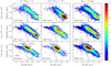 |
Fig. 25. [Mg/Fe] − [Fe/H] distribution for A2A and APOGEE stars in intervals of vertical height (in kpc), for the inner bulge (left column), long bar-outer bulge region (middle column), and within a galactocentric radius of 3.5 kpc (right column). The stars in the first two columns are required to have |Ybar| < 1 kpc. For plot specifics, see the caption of Fig. 24. |
In fact, we see that while the ‘[Fe/H] rich-[Mg/Fe] poor’ stars tend to dominate close to the plane and the ‘[Fe/H] poor-[Mg/Fe] rich’ stars tend to dominate far from the plane, these trends are weaker in the inner bulge than in the long bar-outer bulge region. Instead, in the inner bulge, the ‘[Fe/H] poor-[Mg/Fe] rich’ stars extend lower into the plane and the ‘[Fe/H] rich-[Mg/Fe] poor’ stars extend higher out of the plane than they do in the long bar-outer bulge. This is similar to what we saw in Fig. 24, although now we see it with greater statistics. Many authors take the bulge to be within Rgc < 3.5 kpc. When we apply this distance cut in the third column of Fig. 25 we again see that the ‘[Fe/H] rich-[Mg/Fe] poor’ stars dominate close to the plane while the “[Fe/H] poor-[Mg/Fe] rich” stars dominate far from the plane. Additionally, there is a clear bi-modality for stars with |Z| < 0.5 kpc and 0.5 < |Z| (kpc) < 1. We confirm the clear bi-modality in the [Fe/H] − [Mg/Fe] distribution in the bulge seen by other authors. However, by dividing the bulge into inner bulge and long bar-outer bulge we see that the bi-modal distribution only occurs in the inner bulge. From Fig. 25 we still cannot claim that the two maxima we observe originate from different sequences.
A large fraction of the stars in the inner galaxy are likely contributed by the thin and thick disks. Additionally, a significant fraction of the halo’s stellar mass is thought to reside in the inner galaxy. In Figs. 24 and 25 we draw lines that differentiate regions of the [Mg/Fe] − [Fe/H] space generally populated by the halo, thin disk, and thick disk. These lines are drawn by eye and are similar to those in Adibekyan et al. (2011), Mackereth et al. (2019b), Beraldo e Silva et al. (2021). From examining the stars relative to the lines, we see that stars with abundances similar to the thin disk generally dominate close to the plane while stars with abundances similar to the thick disk generally dominate far from the plane. For small |Xbar|, the ‘[Mg/Fe] poor-[Fe/H] rich’ stars associated with the thin disk dominate at larger |Z| than they do at larger |Xbar|. This could be a result of the thin disk stars being more efficiently mapped to larger |Z| during the buckling episodes that built the b/p bulge. We also see that the stars in the very inner bulge (|Xbar| < 1 kpc and |Z| < 0.3 kpc) are more [Fe/H]-poor and [Mg/Fe]-rich than stars in the neighbouring bins. As these stars reside mainly in the thick disk region, these stars could be thick disk stars. The thick disk is more centrally concentrated than the thin disk and therefore could dominate over the thin disk in the very centre.
Lastly, we want to determine how the Gaussian fits in Sect. 6.3 correspond to the two maxima we see in the [Fe/H] − [Mg/Fe] plane. It is clear from their weight behaviour with position, mean [Fe/H] values, and their correlations to the Mg-DF Gaussians that the MDF Gaussians A and C mainly populate the ‘[Fe/H] rich-[Mg/Fe] poor’ and ‘[Fe/H] poor-[Mg/Fe] rich’ maxima, respectively. Gaussian B from the MDF decomposition appears to be a separate component with strong contamination by the wings of the others.
6.5. Bulge chemo-kinematics
In this section we look at how the radial velocity and dispersion vary with [Fe/H] and field position.
In Fig. 26, we plot the mean velocity (top row) and velocity dispersion (bottom row) of stars against longitude and latitude in different [Fe/H] intervals. In order to increase the number of APOGEE stars at negative longitudes, we use the HQ APOGEE bulge MSp for this analysis, no longer requiring the APOGEE stars to have good SSF estimates. Thus, we include APOGEE stars from fields represented by both the blue ellipses and red crosses in Fig. 1 out to longitudes of ±22°. Because we are including APOGEE stars with no SSF estimates, we do not correct the APOGEE catalogue to the HQ 2MASS catalogue. However, we still correct the A2A catalogue to the HQ 2MASS catalogue it was selected from. Lastly, we restrict the stars to the bulge region by requiring them to have Rgc ≤ 4.5 kpc. The error bars in Fig. 26 were determined using bootstrapping.
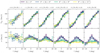 |
Fig. 26. Mean radial velocity (top) and velocity dispersion (bottom) versus longitude and latitude in different [Fe/H] bins. The line colour indicates the latitude range. Dashed lines connect APOGEE fields, and solid lines connect A2A fields. All stars are required to have Rgc < 4.5 kpc. |
We see from Fig. 26 that for stars with [Fe/H] > −1 dex, the mean velocity profiles do not significantly vary with [Fe/H] and that stars in the bulge rotate cylindrically regardless of [Fe/H]. There is a weak trend with latitude where stars located closer to the Galactic plane tend to rotate slightly faster than stars located farther from the Galactic plane. Other studies have observed cylindrical rotation in the bulge (Howard et al. 2009; Kunder et al. 2012; Zoccali et al. 2014) and it is a known property of b/p bulges from N-body simulations (e.g. Athanassoula & Misiriotis 2002; Saha & Gerhard 2013). Below −0.5 dex, the stars rotate more slowly with decreasing [Fe/H]. The stars with [Fe/H] < −1 dex rotate significantly slower than the more [Fe/H]-rich stars.
The velocity dispersion profiles, shown in bottom row of Fig. 26, behave differently with [Fe/H]. Far from the Galactic plane, the shapes of the velocity dispersion profiles are flat for [Fe/H] > −1 dex but the amplitudes increase with decreasing [Fe/H] for −1 < [Fe/H] (dex) < 0. Near the Galactic plane and for [Fe/H] > −0.5 dex, the shapes of the velocity dispersion profiles are high and peaked around |l| = 0°, but the change in amplitude becomes less significant with decreasing [Fe/H]. For stars with [Fe/H] > 0 dex, the dispersion does not change significantly with [Fe/H]. Thus contrary to the velocity profiles, the velocity dispersion profiles of stars with [Fe/H] < 0 dex, do show a clear [Fe/H] dependence.
The dispersion profile of stars with −1 < [Fe/H] (dex) < − 0.5 differs from those with [Fe/H] > −0.5 dex as the separation between latitudes in the inner longitudes is much weaker and the profiles of stars closer to the plane are flatter. However, we see that, as is the case for the more [Fe/H]-rich stars, the increase in dispersion is stronger for the stars at latitudes farther from the plane (|b| > 7.5°). Furthermore, while the dispersion profiles of the stars closer to the plane are flatter than their [Fe/H]-rich counterparts, the distributions of these stars are still peaked around the central longitudes. Therefore, we conclude that the dispersion profiles of stars with −1 < [Fe/H] (dex) < − 0.5 are higher dispersion, slightly flatter versions of the profiles of the stars with [Fe/H] > −0.5 dex.
We find that the stars with −2 < [Fe/H] (dex) < − 1 have different dispersion profiles than the more [Fe/H]-rich stars. Apart from the A2A stars between 3° < |b| < 6°, the dispersion profiles of the low latitude stars are not peaked towards the central longitudes. Furthermore, the dispersion of the stars at large absolute longitudes varies significantly between the different latitudes. The range of [Fe/H], the lower rotation, and higher dispersion is consistent with these stars being part of the halo or very [Fe/H]-poor old thick disk.
We examined the velocity and velocity dispersion profiles of APOGEE stars in the HQSSF APOGEE bulge MSp corrected to the HQ 2MASS catalogue. We find that while the data are noisier due to the lower number of stars and fields, we see similar trends between [Fe/H], kinematics, and positions as in the case when we do not correct for the SSF. Therefore, we believe that the longitude and latitude bins we have chosen are small enough that the effects of the SSF are minimal. As a further check of the effect of the SSF, we compared out results to those of Rojas-Arriagada et al. (2020), who finds using APOGEE DR16 data that the dispersion profiles of the more metal-poor stars with −1.2 < [Fe/H] (dex) < − 0.5 in the bulge (Rgc ≤ 3.5 kpc) are flat even for the stars at latitudes close to the plane. We find that we can reproduce the trends they find, especially those at low metallicities, if we use their metallicity, longitude, and latitude bins. However, using their bins, we find that the dispersion of the very [Fe/H]-rich stars that are close to the plane and near |l| = 0° is lower than what they report. We suspect that this is due to discrepancies on how we correct for the APOGEE SSF. However, this difference is small and we still observe similar trends as Rojas-Arriagada et al. (2020) at the high [Fe/H] end and therefore do not believe the lack of correction for the SSF will significantly affect the main trends we see or the interpretation of our results. Furthermore, the strong agreement we see between the APOGEE and A2A profiles also supports that the effect of the APOGEE SSF is minor.
7. Discussion
Several authors have shown evidence that the presence of a classical bulge in the Milky Way is at most minimal (Shen et al. 2010; Di Matteo et al. 2014; Portail et al. 2017b; Clarke et al. 2019; Queiroz et al. 2020a). Instead, the Milky Way’s bulge is likely to be of mainly disk origin. However, whether the bulge formed from an evolving thin disk, a combination of distinct thin and thick disks, or a disk-continuum is currently debated. N-body models of b/p bulges built from single thin disks with inside-out population gradients have reproduced several characteristics observed in the Milky Way’s b/p bulge, such as cylindrical rotation (Shen et al. 2010) or the vertical metallicity gradient (Martinez-Valpuesta & Gerhard 2011). However, these models also miss many of the finer chemo-kinematic properties seen in the bulge (Di Matteo et al. 2015, 2019; Fragkoudi et al. 2017).
To put further constraints on the formation of the Galactic bulge, we compare the predictions from a number of models exploring different evolutionary scenarios to our principal results.
Bulge iso-[Fe/H] contours. The bulge’s iso-[Fe/H] and iso-[Mg/Fe] contours are X-shaped and exhibit stronger “pinching” than the bulge’s density distribution (see Fig. 16).
Debattista et al. (2017, DB17) presents an evolving single disk model with continuous star formation that evolved to form a bar, which subsequently buckled, forming a b/p bulge. The iso-[Fe/H] contours of the resulting b/p bulge are X-shaped and more pinched than its density distribution. DB17 argues that the stronger pinching of the [Fe/H] distribution in their model is the result of kinematic fractionation, which they define as the separation of stellar populations by the bar due to their different initial radial kinematics. However, Di Matteo et al. (2019, DM19) shows that separation due to differences in vertical dispersion and scale height is similarly important. They created two N-body b/p bulge models using three disks, which either differed in their radial dispersions or in their vertical dispersions and scale heights, but always had the same radial scale lengths. Both models produced b/p bulges with iso-[Fe/H] contours that are X-shaped and more pinched than their density distributions (see their Fig. 5). Lastly, Fragkoudi et al. (2018, F18) built an N-body b/p bulge model initialised from three co-spatial disks each with different kinematics, scale heights, scale lengths, and abundance distributions. The iso-[Fe/H] contours of their final model are also X-shaped and more strongly pinched than the density distribution.
Therefore, we cannot use our result at current resolution to differentiate between the models. However, the stronger pinching of the iso-[Fe/H] contours with respect to the density distribution further verifies that the bulge has a mainly disk origin.
Bulge radial gradient. In the Galactic plane, the Milky Way’s bulge has clear radial gradients in [Fe/H] and [Mg/Fe], such that close to the plane, the inner bulge is more [Fe/H]-poor and [Mg/Fe]-rich than the long bar-outer bulge region; see Figs. 14–17 and 19.
N-body models initialised as a single disk with a strong negative radial metallicity gradient, such as to reproduce the observed vertical gradient in the bulge after bar evolution, inevitably also show a steep radially inward rise in [Fe/H] (Di Matteo et al. 2015; Fragkoudi et al. 2017). Unlike these models, the longitudinal abundance gradient of the multi-disk model of F18 closely matches the gradients we see in Fig. 14 (see their Figs. 9 and 13; already matched to APOGEE DR13 data). This model can reproduce the bulge’s final radial [Fe/H] gradient because the [Fe/H]-poor and [α/Fe]-rich initial disks dominate in the central regions, due to their scale lengths being shorter than that of the [Fe/H]-rich and [α/Fe]-poor disk. On the other hand, the three-disk models of DM19, where all disks were initialised with the same radial scale lengths, show similar or larger final [Fe/H] in their centres than in their in-plane bar regions (see Fig. 5 of DM19). In the star-forming, evolving disk model of DB17, the highest metallicities occur in the centre of the final b/p bulge (see their Figs. 11, 24, and 26). While this model was built from a single disk, before the bar formed the older populations had lower metallicities, as well as larger radial and vertical velocity dispersions and scale heights, than the younger populations, which end up with the largest central concentration.
Thus it appears that the critical ingredient in these models for explaining the radial [Fe/H] gradient in the bulge and bar is the shorter radial scale length of the initial [Fe/H]-poor disk. However, the F18 model assumes a thin disk radial scale length of 4.8 kpc, significantly larger than in current observations (Bland-Hawthorn & Gerhard 2016), and more than twice the thick disk scale length. This suggests other factors are at play as well.
Bovy et al. (2019) and Hasselquist et al. (2020) show age maps for bulge and long bar stars from APOGEE DR16. These maps indicate a significant fraction of younger stars in the long bar and surrounding disk for Rgc > 3.5 kpc and close to the Galactic plane, which are not prominent at smaller radii and at heights above a few 100 pc. This suggests that after the formation of the bulge, the Galactic bar either experienced substantial additional gas inflow and star formation or captured a significant population of disk stars, by slowing its pattern rotation and increasing in size. Capturing disk stars could have happened both intermittently, if indeed the bar regularly changes its pattern speed on dynamical timescales, due to interaction with spiral arms (Hilmi et al. 2020), or secularly by angular momentum transfer to the halo (Chiba & Schönrich 2021). Both mechanisms would be consistent with the dominance of the super-thin bar (Wegg et al. 2015) at these radii. Using the stellar ages from Mackereth et al. (2019a), and restricting the APOGEE sample to ages > 6 Gyr or > 8 Gyr, we still find a horizontal gradient near the disk plane in the remaining bulge sample, but considerably milder. This could be built by a less extreme version of the F18 model, with thin and thick disk scale lengths closer to standard values.
Outer bulge vertical gradient. The vertical [Fe/H] and [Mg/Fe] gradients in the long bar-outer bulge region are ∼ − 0.44 dex kpc−1 and ∼0.13 − 0.17 dex kpc−1, respectively (see Figs. 16 and 18). In this region, there is no inner flattening of the vertical gradient near the plane as is the case in the inner bulge.
For their three-disk models DM19 shows that while both produce b/p bulges, the region beyond the lobes of the b/p bulge in the model formed from the disks with different radial dispersion has no vertical metallicity gradient (see Fig. 6 in DM19). However, in the model built from disks with different vertical scale heights, a vertical gradient remains in the outer bar. The DM19 models are not realistic and are instead designed to represent extreme cases. In reality, the in-plane and vertical dispersions of a disk should be correlated such that a disk with higher (lower) radial dispersion should also have higher (lower) vertical dispersion and therefore a larger (smaller) scale height. The F18 model is more realistic in that the disks with higher dispersions, which are designed to be more [Fe/H]-poor, have larger scale heights. Due to the interplay with the disks’ scale lengths, the F18 model shows a strong vertical gradient in the disk regions.
The single-disk model of Fragkoudi et al. (2017) with an initial radial [Fe/H] gradient does not lead to such a vertical gradient in the outer bar. The evolving disk model, DB17, does show a vertical gradient in the disk. In this model the older populations, which tend to be more metal poor, have larger scale heights than the younger populations, which tend to be metal rich.
This comparison supports a multi-disk formation scenario where the disks that form the bulge must differ in vertical velocity dispersion, and therefore scale height, in order to produce a bulge where the region outside the b/p bulge lobes has strong vertical [Fe/H] and [Mg/Fe] gradients.
The [Fe/H]–[Mg/Fe] distribution. The [Fe/H] − [Mg/Fe] distribution along the bar is roughly linear and composed of two maxima: an ‘[Fe/H] rich-[Mg/Fe] poor’ maximum and an ‘[Fe/H] poor-[Mg/Fe] rich’ maximum. These two maxima vary in strength with position in the bulge such that the [Fe/H]-rich maximum dominates near the plane while the [Fe/H]-poor maximum dominates far from the plane (see Figs. 24 and 25). At small |Xbar|, this trend is also present, although weaker than at larger |Xbar|. There is no clear evidence for two distinct sequences in Figs. 24 and 25 (but see also Queiroz et al. 2020a).
The stronger bi-modality in the [Fe/H] − [α/Fe] distribution is often interpreted as two distinct star formation episodes well separated by a period of quenched star formation (Chiappini et al. 1997; Haywood et al. 2018). The APOGEE DR16 [Fe/H] − [Mg/Fe] distribution of the bulge (Rgc < 3 kpc and |Z| < 0.5 kpc) was recently modelled by Lian et al. (2020) using a chemical evolution model with an early period of high star formation, which formed the high [Mg/Fe] stars, followed by a quick star formation quenching episode and a long lived period of low star formation, which formed the low [Mg/Fe] stars. This model reproduces the [Fe/H] − [Mg/Fe] distribution of the inner bulge (see Fig. 25) and the bi-modal Mg-DFs of the inner bulge seen in APOGEE (Fig. 20) (see also Matteucci et al. 2019).
Kinematics with metallicity along the [Fe/H]–[Mg/Fe] distribution. The stars composing the two maxima in the [Fe/H] − [Mg/Fe] distribution display different kinematics. Specifically, the stars in the [Fe/H]-rich maximum (mainly [Fe/H] > 0 dex) are kinematically colder than the stars in the [Fe/H]-poor maximum (mainly −1 < [Fe/H] (dex) < − 0.25). Furthermore, the stars composing the [Fe/H]-rich maximum have little kinematic-[Fe/H] dependence while the stars composing the [Fe/H]-poor maximum rotate slightly slower and increase in dispersion with decreasing [Fe/H] (see Fig. 26).
Di Matteo et al. (2015) shows using an N-body model that if the origin of a b/p bulge is a single disk with a strong negative radial [Fe/H] gradient, then the [Fe/H]-poor stars should rotate faster than, and have warmer, although similarly shaped, velocity dispersion profiles to the [Fe/H]-rich stars as in this scenario the [Fe/H]-poor stars originate from larger disk radii. The lack of kinematic dependence on [Fe/H] of the stars in the [Fe/H]-rich maximum and the decrease in mean velocity with decreasing [Fe/H] in the [Fe/H]-poor maximum indicates that the origin of the Galactic bulge cannot be a single disk with a strong negative radial [Fe/H] gradient. Instead, kinematic and spatial differences of the maxima support a scenario where the stars composing the maxima originate from at least two separate disks, with the stars composing the [Fe/H]-rich maximum originating from a colder disk with little to no radial [Fe/H] gradient and the stars composing the [Fe/H]-poor maximum originating from a hotter disk.
DB17 finds that in order for the stars with [Fe/H] < −0.5 dex in their model to have the high, flat, and largely latitude-independent dispersion profiles observed in Ness et al. (2013a), they need to add a slowly rotating, low mass (5% central Milky Way mass), high dispersion component to their model. They associated this component with the stellar halo (see their Fig. 21). From our data, the slower rotation and increased dispersion of the stars with −1 < [Fe/H] (dex) < − 0.5 as compared to the stars with −0.5 < [Fe/H] (dex) < − 0.25 may be the result of contamination by the high dispersion component dominating below −1 dex. As the stars in the [Fe/H]-poor tail are slowly rotating, kinematically hot, and [Mg/Fe]-rich, we tentatively associate them with the stellar halo. A contamination by halo stars is further supported by Lucey et al. (2021) who, from examining the chemo-kinematics of metal-poor bulge stars, finds that the fraction of halo interlopers in the bulge increases with decreasing metallicity between −3 < [Fe/H] (dex) < 0.5.
In all, our data paints a consistent picture for the origin of the b/p bulge: at least two initial disks with differing dispersions, scale heights, and scale lengths underwent spatial and kinematic fractionation resulting in the b/p bulge of the Milky Way that we observe today. Due to their kinematics as well as their [Fe/H] − [Mg/Fe] distributions, we associate these disks with the thin and thick disks. We also associate the very [Fe/H]-poor, [Mg/Fe]-rich, kinematically hot tail of the bulge stars with the stellar halo.
8. Summary and conclusions
In this work we used the data-driven method The Cannon to put stars from the ARGOS survey onto the parameter and abundance scales of the APOGEE survey. After doing so, we were able to directly combine the two surveys and gain a deeper and more reliable coverage of the Galactic bulge.
In the first half of the paper, we described how we applied The Cannon to the ARGOS stars to obtain the A2A survey. To show that we have successfully placed the A2A stars on the APOGEE label scales, we performed three validation tests: the pick-one-out test (Fig. 4), spectrum reconstruction (Fig. 5), and stellar Teff − log(g) distribution (Fig. 7). These tests show that it is possible to perform The Cannon label transfer using a moderate number (204) of reference set stars and still obtain labels with good precisions. After performing the validation tests, we accounted for the SSF of each survey such that, after it was corrected for, we statistically obtained the HQ 2MASS catalogues they were selected from. After this, we compared the SSF-corrected MDFs and Mg-DFs of the APOGEE and A2A surveys and found that the different spatial regions probed by each survey cause a clear spatial bias; however, when the distribution functions were compared in fixed distance bins, the MDFs and Mg-DFs agreed except at the high [Mg/Fe] and low [Fe/H] ends, where APOGEE observes more stars. This may be due to trends between Teff and the abundances in APOGEE and the fact that the reference set only covers a limited Teff range on the APOGEE scale.
In the second half of the paper, we used stars from both the A2A and APOGEE surveys to investigate the abundance structure of the bulge. The results we found include:
-
The [Fe/H] and [Mg/Fe] maps built using APOGEE and A2A data show strong X-shapes that are more pinched than the density distribution given by the currently best dynamical model of the Milky Way’s bulge and bar from Portail et al. (2017a). The stronger pinching in the [Fe/H] and [Mg/Fe] maps than in the density map supports a mainly disk origin for the Galactic bulge.
-
The inner bulge and long bar-outer bulge region have different chemical properties. While the inner bulge [Fe/H] and [Mg/Fe] profiles are nearly flat within 0.7 kpc of the Galactic plane and then steepen to ∼ − 0.41 dex kpc−1 and ∼0.11 dex kpc−1, respectively, the vertical [Fe/H] and [Mg/Fe] profiles of the long bar-outer bulge region are steep near the plane at ∼ − 0.44 dex kpc−1 and ∼0.13 − 0.17 dex kpc−1, respectively, with a flat distribution for |Z| > 1.25 kpc. Close to the plane the inner bulge is sub-solar in [Fe/H] and [Mg/Fe]-rich, while the flat bar is nearly solar in [Fe/H] and [Mg/Fe]-normal.
-
The [Fe/H] − [Mg/Fe] distributions in the bulge and long bar have two main maxima, an ‘[Fe/H] rich-[Mg/Fe] poor’ maximum and an ‘[Fe/H] poor-[Mg/Fe] rich’ maximum. The ‘[Fe/H] rich-[Mg/Fe] poor’ maximum dominates close to the plane, has a lower dispersion, and shows no significant mean radial velocity dependence on [Fe/H]. The ‘[Fe/H] poor-[Mg/Fe] rich’ maximum dominates far from the plane, has a higher dispersion, and its [Fe/H]-poorer stars rotate slightly more slowly on average than its [Fe/H]-richer stars.
-
The most [Fe/H]-poor stars ([Fe/H] < −1 dex) rotate slowly and have high flat dispersion profiles. We associate these stars with the stellar halo. This is also supported by the distribution of these [Fe/H]-poor stars in the [Fe/H] − [Mg/Fe] plane in Fig. 24.
The positive horizontal [Fe/H] gradient in the bulge close to the Galactic plane and the negative vertical [Fe/H] gradient in the long bar region favour models in which the bulge and bar formed from initial thin and thick disks with different vertical and radial scale lengths (Fragkoudi et al. 2018). This multi-disk origin is further supported by the higher pinching of the abundance distributions in the bulge as compared to the density distributions and the differing kinematics of the low and high [Fe/H] stars. However, the large thin-disk scale lengths required by these models, together with younger estimated mean ages in the outer bar (Bovy et al. 2019; Hasselquist et al. 2020), suggest that the Galactic bar may have captured younger, more metal-rich stars well after its formation.
Cohort magnitude limits were set depending on the planned number of visits. Most cohorts used in this work have the magnitude limits 7 < H0 (mag) < 11, 7 < H0 (mag) < 12.2, or 7 < H0 (mag) < 12.8, although some have fainter limits. The colour limits of the cohorts are (J − Ks)0 ≥ 0.5 mag in bulge and APOGEE-1 disk fields, and 0.5 ≤ (J − Ks)0 (mag) ≤ 0.8 and (J − Ks)0 > 0.8 mag in APOGEE-2 disk fields; see Zasowski et al. (2017).
Acknowledgments
J. Bland-Hawthorn is funded by an ARC Laureate Fellowship that partially supports the GALAH survey science team. Funding for the Sloan Digital Sky Survey IV has been provided by the Alfred P. Sloan Foundation, the US Department of Energy Office of Science, and the Participating Institutions. SDSS-IV acknowledges support and resources from the Centre for High-Performance Computing at the University of Utah. The SDSS website is www.sdss.org. SDSS-IV is managed by the Astrophysical Research Consortium for the Participating Institutions of the SDSS Collaboration including the Brazilian Participation Group, the Carnegie Institution for Science, Carnegie Mellon University, the Chilean Participation Group, the French Participation Group, Harvard-Smithsonian Centre for Astrophysics, Instituto de Astrofísica de Canarias, The Johns Hopkins University, Kavli Institute for the Physics and Mathematics of the Universe (IPMU)/University of Tokyo, the Korean Participation Group, Lawrence Berkeley National Laboratory, Leibniz Institut für Astrophysik Potsdam (AIP), Max-Planck-Institut für Astronomie (MPIA Heidelberg), Max-Planck-Institut für Astrophysik (MPA Garching), Max-Planck-Institut für Extraterrestrische Physik (MPE), National Astronomical Observatories of China, New Mexico State University, New York University, University of Notre Dame, Observatário Nacional/MCTI, The Ohio State University, Pennsylvania State University, Shanghai Astronomical Observatory, United Kingdom Participation Group, Universidad Nacional Autónoma de México, University of Arizona, University of Colorado Boulder, University of Oxford, University of Portsmouth, University of Utah, University of Virginia, University of Washington, University of Wisconsin, Vanderbilt University, and Yale University.
References
- Adibekyan, V. Z., Santos, N. C., Sousa, S. G., & Israelian, G. 2011, A&A, 535, L11 [NASA ADS] [CrossRef] [EDP Sciences] [Google Scholar]
- Ahumada, R., Prieto, C. A., Almeida, A., et al. 2020, ApJS, 249, 3 [Google Scholar]
- Alam, S., Albareti, F. D., Allende Prieto, C., et al. 2015, ApJS, 219, 12 [NASA ADS] [CrossRef] [Google Scholar]
- Allende Prieto, C., Beers, T. C., Wilhelm, R., et al. 2006, ApJ, 636, 804 [NASA ADS] [CrossRef] [Google Scholar]
- Alves, D. R. 2000, ApJ, 539, 732 [NASA ADS] [CrossRef] [MathSciNet] [Google Scholar]
- Athanassoula, E., & Misiriotis, A. 2002, MNRAS, 330, 35 [NASA ADS] [CrossRef] [Google Scholar]
- Bensby, T., Yee, J. C., Feltzing, S., et al. 2013, A&A, 549, A147 [NASA ADS] [CrossRef] [EDP Sciences] [Google Scholar]
- Bensby, T., Feltzing, S., Gould, A., et al. 2017, A&A, 605, A89 [NASA ADS] [CrossRef] [EDP Sciences] [Google Scholar]
- Beraldo e Silva, L., Debattista, V. P., Nidever, D., Amarante, J. A. S., & Garver, B. 2021, MNRAS, 502, 260 [NASA ADS] [CrossRef] [Google Scholar]
- Bessell, M. S., Castelli, F., & Plez, B. 1998, A&A, 333, 231 [NASA ADS] [Google Scholar]
- Birky, J., Hogg, D. W., Mann, A. W., & Burgasser, A. 2020, ApJ, 892, 31 [Google Scholar]
- Bland-Hawthorn, J., & Gerhard, O. 2016, ARA&A, 54, 529 [NASA ADS] [CrossRef] [EDP Sciences] [Google Scholar]
- Bovy, J. 2016, ApJ, 817, 49 [NASA ADS] [CrossRef] [Google Scholar]
- Bovy, J., Nidever, D. L., Rix, H.-W., et al. 2014, ApJ, 790, 127 [NASA ADS] [CrossRef] [Google Scholar]
- Bovy, J., Leung, H. W., Hunt, J. A. S., et al. 2019, MNRAS, 490, 4740 [Google Scholar]
- Bressan, A., Marigo, P., Girardi, L., et al. 2012, MNRAS, 427, 127 [NASA ADS] [CrossRef] [Google Scholar]
- Casey, A. R., Hawkins, K., Hogg, D. W., et al. 2017, ApJ, 840, 59 [NASA ADS] [CrossRef] [Google Scholar]
- Chen, Y., Girardi, L., Bressan, A., et al. 2014, MNRAS, 444, 2525 [NASA ADS] [CrossRef] [Google Scholar]
- Chen, Y., Bressan, A., Girardi, L., et al. 2015, MNRAS, 452, 1068 [NASA ADS] [CrossRef] [Google Scholar]
- Chiappini, C., Matteucci, F., & Gratton, R. 1997, ApJ, 477, 765 [Google Scholar]
- Chiba, R., & Schönrich, R. 2021, MNRAS, 505, 2412 [NASA ADS] [CrossRef] [Google Scholar]
- Clarke, J. P., Wegg, C., Gerhard, O., et al. 2019, MNRAS, 489, 3519 [NASA ADS] [CrossRef] [Google Scholar]
- Cropper, M., Katz, D., Sartoretti, P., et al. 2018, A&A, 616, A5 [NASA ADS] [CrossRef] [EDP Sciences] [Google Scholar]
- Debattista, V. P., Ness, M., Gonzalez, O. A., et al. 2017, MNRAS, 469, 1587 [NASA ADS] [CrossRef] [Google Scholar]
- Di Matteo, P., Haywood, M., Gómez, A., et al. 2014, A&A, 567, A122 [NASA ADS] [CrossRef] [EDP Sciences] [Google Scholar]
- Di Matteo, P., Gómez, A., Haywood, M., et al. 2015, A&A, 577, A1 [NASA ADS] [CrossRef] [EDP Sciences] [Google Scholar]
- Di Matteo, P., Fragkoudi, F., Khoperskov, S., et al. 2019, A&A, 628, A11 [CrossRef] [EDP Sciences] [Google Scholar]
- Foreman-Mackey, D., Hogg, D. W., Lang, D., & Goodman, J. 2013, PASP, 125, 306 [Google Scholar]
- Fragkoudi, F., Di Matteo, P., Haywood, M., et al. 2017, A&A, 607, L4 [NASA ADS] [CrossRef] [EDP Sciences] [Google Scholar]
- Fragkoudi, F., Di Matteo, P., Haywood, M., et al. 2018, A&A, 616, A180 [NASA ADS] [CrossRef] [EDP Sciences] [Google Scholar]
- Freeman, K., Ness, M., Wylie-de Boer, E., et al. 2012, MNRAS, 428, 3660 [Google Scholar]
- Gaia Collaboration (Brown, A. G. A., et al.) 2018, A&A, 616, A1 [NASA ADS] [CrossRef] [EDP Sciences] [Google Scholar]
- Galgano, B., Stassun, K., & Rojas-Ayala, B. 2020, AJ, 159, 193 [NASA ADS] [CrossRef] [Google Scholar]
- García Pérez, A. E., Prieto, C. A., Holtzman, J. A., et al. 2016, AJ, 151, 144 [NASA ADS] [CrossRef] [Google Scholar]
- Gilmore, G., Randich, S., Asplund, M., et al. 2012, The Messenger, 147, 25 [NASA ADS] [Google Scholar]
- Hasselquist, S., Zasowski, G., Feuillet, D. K., et al. 2020, ApJ, 901, 109 [CrossRef] [Google Scholar]
- Hayden, M. R., Bovy, J., Holtzman, J. A., et al. 2015, ApJ, 808, 132 [Google Scholar]
- Haywood, M., Di Matteo, P., Lehnert, M., et al. 2018, A&A, 618, A78 [NASA ADS] [CrossRef] [EDP Sciences] [Google Scholar]
- Hill, V., Lecureur, A., Gómez, A., et al. 2011, A&A, 534, A80 [NASA ADS] [CrossRef] [EDP Sciences] [Google Scholar]
- Hilmi, T., Minchev, I., Buck, T., et al. 2020, MNRAS, 497, 933 [CrossRef] [Google Scholar]
- Ho, A. Y. Q., Ness, M. K., Hogg, D. W., et al. 2017, ApJ, 836, 5 [NASA ADS] [CrossRef] [Google Scholar]
- Holtzman, J. A., Hasselquist, S., Shetrone, M., et al. 2018, AJ, 156, 125 [Google Scholar]
- Horta, D., Schiavon, R. P., Mackereth, J. T., et al. 2021, MNRAS, 500, 1385 [CrossRef] [Google Scholar]
- Howard, C. D., Rich, R. M., Clarkson, W., et al. 2009, ApJ, 702, L153 [NASA ADS] [CrossRef] [Google Scholar]
- Jofré, P., Heiter, U., & Soubiran, C. 2019, ARA&A, 57, 571 [Google Scholar]
- Jönsson, H., Allende Prieto, C., Holtzman, J. A., et al. 2018, AJ, 156, 126 [Google Scholar]
- Jönsson, H., Holtzman, J. A., Allende Prieto, C., et al. 2020, AJ, 160, 120 [CrossRef] [Google Scholar]
- Kunder, A., Koch, A., Michael Rich, R., et al. 2012, AJ, 143, 57 [NASA ADS] [CrossRef] [Google Scholar]
- Leung, H. W., & Bovy, J. 2019, MNRAS, 489, 2079 [NASA ADS] [CrossRef] [Google Scholar]
- Lian, J., Zasowski, G., Hasselquist, S., et al. 2020, MNRAS, 497, 3557 [NASA ADS] [CrossRef] [Google Scholar]
- Lucey, M., Hawkins, K., Ness, M., et al. 2021, MNRAS, 501, 5981 [NASA ADS] [CrossRef] [Google Scholar]
- Mackereth, J. T., & Bovy, J. 2020, MNRAS, 492, 3631 [CrossRef] [Google Scholar]
- Mackereth, J. T., Bovy, J., Leung, H. W., et al. 2019a, MNRAS, 489, 176 [CrossRef] [Google Scholar]
- Mackereth, J. T., Schiavon, R. P., Pfeffer, J., et al. 2019b, MNRAS, 482, 3426 [NASA ADS] [CrossRef] [Google Scholar]
- Majewski, S. 2016, Astron. Nachr., 337, 863 [Google Scholar]
- Martinez-Valpuesta, I., & Gerhard, O. 2011, ApJ, 734, L20 [NASA ADS] [CrossRef] [Google Scholar]
- Matteucci, F., Grisoni, V., Spitoni, E., et al. 2019, MNRAS, 487, 5363 [Google Scholar]
- Minniti, D., Lucas, P. W., Emerson, J. P., et al. 2010, New Astron., 15, 433 [Google Scholar]
- Ness, M., Freeman, K., Athanassoula, E., et al. 2013a, MNRAS, 432, 2092 [NASA ADS] [CrossRef] [Google Scholar]
- Ness, M., Freeman, K., Athanassoula, E., et al. 2013b, MNRAS, 430, 836 [NASA ADS] [CrossRef] [Google Scholar]
- Ness, M., Hogg, D. W., Rix, H.-W., Ho, A. Y. Q., & Zasowski, G. 2015, ApJ, 808, 16 [NASA ADS] [CrossRef] [Google Scholar]
- Ness, M., Zasowski, G., Johnson, J. A., et al. 2016, ApJ, 819, 2 [NASA ADS] [CrossRef] [Google Scholar]
- Plez, B. 2012, Astrophysics Source Code Library [record ascl:1205.004] [Google Scholar]
- Plez, B., Brett, J. M., & Nordlund, A. 1992, A&A, 256, 551 [NASA ADS] [Google Scholar]
- Portail, M., Gerhard, O., Wegg, C., & Ness, M. 2017a, MNRAS, 465, 1621 [NASA ADS] [CrossRef] [Google Scholar]
- Portail, M., Wegg, C., Gerhard, O., & Ness, M. 2017b, MNRAS, 470, 1233 [NASA ADS] [CrossRef] [Google Scholar]
- Queiroz, A. B. A., Chiappini, C., Perez-Villegas, A., et al. 2020a, A&A, submitted [arXiv:2007.12915] [Google Scholar]
- Queiroz, A. B. A., Anders, F., Chiappini, C., et al. 2020b, A&A, 638, A76 [CrossRef] [EDP Sciences] [Google Scholar]
- Rich, R. M., Origlia, L., & Valenti, E. 2007, ApJ, 665, L119 [NASA ADS] [CrossRef] [Google Scholar]
- Rich, R. M., Origlia, L., & Valenti, E. 2012, ApJ, 746, 59 [NASA ADS] [CrossRef] [Google Scholar]
- Rojas-Arriagada, A., Recio-Blanco, A., Hill, V., et al. 2014, A&A, 569, A103 [NASA ADS] [CrossRef] [EDP Sciences] [Google Scholar]
- Rojas-Arriagada, A., Recio-Blanco, A., de Laverny, P., et al. 2017, A&A, 601, A140 [NASA ADS] [CrossRef] [EDP Sciences] [Google Scholar]
- Rojas-Arriagada, A., Zoccali, M., Schultheis, M., et al. 2019, A&A, 626, A16 [NASA ADS] [CrossRef] [EDP Sciences] [Google Scholar]
- Rojas-Arriagada, A., Zasowski, G., Schultheis, M., et al. 2020, MNRAS, 499, 1037 [CrossRef] [Google Scholar]
- Saha, K., & Gerhard, O. 2013, MNRAS, 430, 2039 [NASA ADS] [CrossRef] [Google Scholar]
- Schlafly, E. F., & Finkbeiner, D. P. 2011, ApJ, 737, 103 [NASA ADS] [CrossRef] [Google Scholar]
- Schlegel, D. J., Finkbeiner, D. P., & Davis, M. 1998, ApJ, 500, 525 [NASA ADS] [CrossRef] [Google Scholar]
- Schultheis, M., Rojas-Arriagada, A., García Pérez, A. E., et al. 2017, A&A, 600, A14 [NASA ADS] [CrossRef] [EDP Sciences] [Google Scholar]
- Scott, D. W. 1992, Multivariate Density Estimation (New York: Wiley) [Google Scholar]
- Sharma, S., Bland-Hawthorn, J., Johnston, K. V., & Binney, J. 2011, ApJ, 730, 3 [NASA ADS] [CrossRef] [Google Scholar]
- Shen, J., Rich, R. M., Kormendy, J., et al. 2010, ApJ, 720, L72 [NASA ADS] [CrossRef] [Google Scholar]
- Skrutskie, M. F., Cutri, R. M., Stiening, R., et al. 2006, AJ, 131, 1163 [NASA ADS] [CrossRef] [Google Scholar]
- Sneden, C., Bean, J., Ivans, I., Lucatello, S., & Sobeck, J. 2012, Astrophysics Source Code Library [record ascl:1202.009] [Google Scholar]
- Surot, F., Valenti, E., Hidalgo, S. L., et al. 2019, A&A, 629, A1 [NASA ADS] [CrossRef] [EDP Sciences] [Google Scholar]
- Tang, J., Bressan, A., Rosenfield, P., et al. 2014, MNRAS, 445, 4287 [NASA ADS] [CrossRef] [Google Scholar]
- Uttenthaler, S., Schultheis, M., Nataf, D. M., et al. 2012, A&A, 546, A57 [NASA ADS] [CrossRef] [EDP Sciences] [Google Scholar]
- Wegg, C., Gerhard, O., & Portail, M. 2015, MNRAS, 450, 4050 [NASA ADS] [CrossRef] [Google Scholar]
- Wheeler, A., Ness, M., Buder, S., et al. 2020, ApJ, 898, 58 [Google Scholar]
- Zasowski, G., Cohen, R. E., Chojnowski, S. D., et al. 2017, AJ, 154, 198 [NASA ADS] [CrossRef] [Google Scholar]
- Zoccali, M., Gonzalez, O. A., Vasquez, S., et al. 2014, A&A, 562, A66 [NASA ADS] [CrossRef] [EDP Sciences] [Google Scholar]
- Zoccali, M., Vasquez, S., Gonzalez, O. A., et al. 2017, A&A, 599, A12 [NASA ADS] [CrossRef] [EDP Sciences] [Google Scholar]
Appendix A: Effect of log(g) limits on the A2A red clump sample completeness
We can approximate the effect of the log(g) limits (8b) on the completeness of the A2A RC stars. In the top plot of Fig. A.1, the cyan histogram shows the number of ARGOS stars as a function of ARGOS log(g). The colour cut in Eq. 12 and reference set limits 7a, 8a, 8b have been applied. The gravity reference set limit 8b has not been applied. The blue histogram in the top plot of Fig. A.1 gives the number of A2A RC stars at each ARGOS log(g). It should be noticed that because the blue histogram is built from A2A stars, the log(g) limits (8b) have been applied and the blue histogram does not extend as far in log(g) as the cyan histogram. In the bottom plot of Fig. A.1, we take the ratio of the two histograms to get the fraction of A2A RC stars at each ARGOS log(g). At log(g) = 2.6 dex, 55.5% of the stars in the cyan histogram are A2A RC stars. The fraction decreases linearly outwards in both directions to 31% at 1.6 dex and 38.0% at 3.2 dex. We ignore the final bins because the log(g) limits fall within these bins causing the number of RC stars to be artificially lower. Assuming the linear trend on both sides continues past the limits, we fit a line to each side and extrapolated beyond the cuts to get the fraction of RC stars at each ARGOS log(g). We then multiplied the number of stars given by the cyan histogram in the outer bins by the fractions we got from extrapolating to get the approximate number of RC stars removed by the log(g) limits. Using this method, we find that approximately 200 RC stars are removed by the log(g) limits. Under the assumption that, to the first order, the other limits (7a, 8a, and 8b) affect the RC and non-RC stars equally, then 92% of the RC stars originally observed by ARGOS are accounted for in the A2A catalogue.
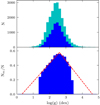 |
Fig. A.1. Effect of the ARGOS log(g) limits on the completness of the RC in A2A. Top: Number of stars as a function of ARGOS log(g). The cyan histogram gives the number of stars after the Teff, [Mg/Fe], [Fe/H], and colour limits (7a, 8a, 8b, and 12) have been applied. The blue histogram gives the number of A2A RC stars per ARGOS log(g) bin. Bottom: Fraction of A2A RC stars as a function of ARGOS gravity (ratio of blue to cyan histogram in the top plot). The red lines are linear fits to the distribution. |
Appendix B: Abundance trends in APOGEE and the effect on A2A
It has been found in APOGEE that the ASPCAP Teff is correlated with some of the ASPCAP abundances due to the physical stellar models (Jönsson et al. 2018; Jofré et al. 2019). We show the correlation between Teff and [Mg/Fe] of stars in bins of [Fe/H] in Fig. B.1. For all plots, the stars are restricted to narrow ranges in distance, S/N, and height from the plane. The reference set we use to train The Cannon model to build the A2A catalogue does not span the entire Teff range covered by the HQSSF APOGEE bulge MSp (see Fig. B.2).
 |
Fig. B.1. ASPCAP Teff-[Mg/Fe] distribution of APOGEE stars in different [Fe/H] bins with 6 < Ds (kpc) < 8, |Z| < 1 kpc, and 100 < S/N < 200. The red line gives the running mean of the distribution, while the blue shaded area gives the Teff range spanned by the reference set on the APOGEE scale. |
 |
Fig. B.2. Teff distributions of the HQSSF APOGEE bulge MSp and of the reference set used to put the A2A survey on the APOGEE parameter scale. |
All Figures
|
Fig. 1. Locations of the APOGEE (blue ellipses and red crosses) and ARGOS (green ellipses) bulge fields. The red crosses indicate APOGEE fields that either have no or poor SSF estimates. The marker size indicates the field size. |
| In the text | |
|
Fig. 2. APOGEE-derived parameters (x axis) versus ARGOS derived parameters (y axis) for the 204 reference set stars observed by both surveys. The bias (mean of the differences) and rms of the distributions are given in the upper left hand corner of each plot. The reference set stars that are within one ARGOS observational error, 0.13 dex (0.1 dex), from the maximum [Fe/H] ([α/Fe]) value reached by the reference set are plotted as blue crosses (red triangles). |
| In the text | |
|
Fig. 3. Comparison of the [Fe/H] (top) and [Mg/Fe] (bottom) labels generated by the original Cannon model (x axis) and the m1σ models (y axis). In the top plot, only stars with ARGOS 0.05 < [Fe/H] (dex) < 0.18 are compared (the region in [Fe/H] spanned by the blue crosses in the top plot of Fig. 2). In the bottom plot, only stars with ARGOS 0.47 < [α/Fe] (dex) < 0.57 are compared (the region in [α/Fe] spanned by the red triangles in the plot second from the top in Fig. 2). The points are coloured by the point density. The black lines are one-to-one lines, and blue lines indicate ±1σARG. The bias and rms of each distribution are given in the top left corner of each plot. |
| In the text | |
|
Fig. 4. Pick-one-out test. For each plot, each point represents a different reference set star. For a given point in a plot, the x axis value is the APOGEE-derived label and the y axis value is the label prediction from a Cannon model trained on all other (203) reference set stars. Therefore, for each point in each plot, the applied Cannon model is different than that of every other point. The points are coloured by their model χ2 values. The bias and rms of each distribution are given in the top left corner of each plot. |
| In the text | |
|
Fig. 5. Normalised ARGOS spectra (black) versus the normalised model spectra (blue) generated by The Cannon for A2A stars with [Fe/H] values between −0.5 ≲ [Fe/H] ≲ 0.25. The plotted line thicknesses of the model spectra indicate the scatter of each fit by The Cannon. The residuals between the normalised ARGOS spectra and normalised model spectra are also shown in the panels below the spectra. |
| In the text | |
|
Fig. 6. Model χ2 distribution of A2A stars. The dashed orange line gives the number of pixels in each ARGOS spectrum. |
| In the text | |
|
Fig. 7. Teff − log(g) distribution of ARGOS (left) and A2A (right) stars coloured by mean [Fe/H]. 10 Gyr PARSEC isochrones with −2 < [Fe/H] (dex) < 0.6 are plotted beneath. We note that the isochrones are plotted at 35% transparency in order to visually differentiate them from the 2D histograms. |
| In the text | |
|
Fig. 8. Normalised ARGOS and A2A MDFs of all stars (top) and RC stars (bottom). The grey histogram includes stars from the full ARGOS catalogue, while the teal histogram includes only ARGOS stars that could be processed by The Cannon (same stars as in the A2A catalogue but with their old ARGOS labels). |
| In the text | |
|
Fig. 9. Original and weighted Ks0-band LFs of ARGOS (top) and A2A (bottom) stars in the field (l, b) = (−10° , − 10° ). The HQ 2MASS LF is also plotted. The colour limits 0.45 ≤ (J − Ks)0 (mag)≤0.86 are applied to the LFs in the bottom plot. The A2A LF is slightly below the HQ 2MASS LF due to the parametric limits applied during the creation of the A2A catalogue. |
| In the text | |
|
Fig. 10. ARGOSTeff versus de-reddened colour distribution of the full ARGOS catalogue. The point colour indicates the ARGOS [Fe/H]. The blue vertical lines show the reference set Teff limits (7a). The blue horizontal lines show the colour limits (12) used to approximate the Teff limits. |
| In the text | |
|
Fig. 11. Original and weighted APOGEEH-band LFs of the HQSSF bulge MSp for a cohort in the field (l, b) = (−2° ,0° ). The HQ 2MASS LF is also plotted. |
| In the text | |
|
Fig. 12. MDFs of bright and faint stars in the same distance bins. Top: A2A RC stars from the field (l, b) = (0° , − 5° ) and the distance bin 6 to 8 kpc with the weights from Eq. (11) applied. Bottom: APOGEE stars from the field (l, b) = (0° , − 2° ) and the distance bin 6 to 8 kpc with the weights from Eqs. (13) and (14) applied. The number of stars in each MDF is given in the legend of each plot. The means of each histogram are given by the triangular markers. |
| In the text | |
|
Fig. 13. SSF-corrected MDFs (first column), Mg-DFs (second column), and their respective positional information (third and fourth columns) of A2A and APOGEE stars with [Fe/H] > −1 dex. The top row includes all stars in each catalogue, while the stars in the second and third rows are restricted to successively smaller areas. The A2A stars are restricted to RC stars. The mean [Fe/H] and [Mg/Fe] values of each MDF and Mg-DF are shown by the triangular markers in each plot. |
| In the text | |
|
Fig. 14. SSF-corrected mean [Fe/H] (left) and [Mg/Fe] (right) in APOGEE (circles) and A2A (squares) fields for stars with [Fe/H] > −1 dex and distances from the Sun between 4 and 12 kpc. |
| In the text | |
|
Fig. 15. SSF-corrected mean [Fe/H] distributions in the X − Z plane (top row) and X − Y plane (bottom row) of A2A (left column), APOGEE (middle column), and combined (right column) stars with [Fe/H] > −1 dex. The red lines trace the density distribution of the Milky Way’s bar obtained from a Portail et al. (2017a) bulge-bar model. The red star in each plot marks the position of the Sun. |
| In the text | |
|
Fig. 16. SSF-corrected symmetrised mean [Fe/H] (top row) and [Mg/Fe] (bottom row) distribution in the Xbar − Z plane for combined A2A and APOGEE stars with [Fe/H] > −1 dex in slices of |Ybar|. The dotted white lines trace the density distribution obtained from a Portail et al. (2017a) bulge-bar model. The red arrow points in the direction of the Sun. |
| In the text | |
|
Fig. 17. SSF-corrected symmetrised mean [Fe/H] distribution in vertical slices along the Galactic bar for combined A2A and APOGEE stars with [Fe/H] > −1 dex. The red arrow points in the direction of the Sun. |
| In the text | |
|
Fig. 18. SSF-corrected mean [Fe/H] (top row) and [Mg/Fe] (bottom row) vertical abundance profiles for A2A and APOGEE stars in the inner b/p bulge (|Xbar| < 2 kpc, |Ybar| < 1 kpc; left) and long bar-outer bulge regions (2.5 kpc | ≤ Xbar| < 4.5 kpc, |Ybar| < 1 kpc; right). The A2A and APOGEE gradients of the regions shown by the teal and purple lines are given in the legend of each diagram; error ranges of the linear fits are shown by the shaded regions. For all plots, we require the stars to have [Fe/H] > −1 dex. |
| In the text | |
|
Fig. 19. SSF-corrected mean [Fe/H] (top row) and [Mg/Fe] (bottom row) horizontal abundance profiles of A2A and APOGEE stars along the bar and at different heights above the Galactic plane. For all plots, we require the stars to have [Fe/H] > −1 dex and |Ybar| < 1 kpc. |
| In the text | |
|
Fig. 20. Generalised MDFs (left two columns) and Mg-DFs (right two columns) of A2A (RC) and APOGEE stars at different absolute heights above the plane in the inner bulge, shown as filled distributions in green. The stars are required to have |Xbar| < 2 kpc, |Ybar| < 1 kpc, and [Fe/H] > −1 dex. Gaussian mixture decompositions at each height are also shown, in black (individual Gaussians and sums). The number of distinct stars composing each distribution is given in each plot. The number in brackets in the A2A plots gives the number (total weight) of A2A RC stars. |
| In the text | |
|
Fig. 21. Variation in the Gaussian parameters with height from the Galactic plane (|Z|) for the inner bulge. Top row: parameters from the MDF decompositions. Bottom row: parameters from the Mg-DF decompositions. The lines connect points with at least 300 distinct stars. Triangular markers and solid lines show the A2A decompositions. Circular markers and dashed lines show the APOGEE decompositions. |
| In the text | |
|
Fig. 22. Same as Fig. 20 except for the long bar-outer bulge region. The stars are required to have 2.5 kpc ≤ |Xbar| < 4.5 kpc, |Ybar| < 1 kpc, and [Fe/H] > −1 dex. |
| In the text | |
 |
Fig. 23. Same as Fig. 21 except for the long bar-outer bulge region. |
| In the text | |
|
Fig. 24. [Mg/Fe] − [Fe/H] distribution of A2A and APOGEE stars in intervals of height from the plane (|Z|, kpc) and distance along the bar (|Xbar|, kpc). The stars are required to have |Ybar| < 1 kpc. The point colour gives the Gaussian kernel density estimate. The dashed lines separate the different regions in the parameter space generally populated by the halo, thin disk, and thick disk (defined in the lower-leftmost plot; see text). The number of stars composing each plot (A2A RC stars + APOGEE stars) is given in the lower left corner of each plot. |
| In the text | |
|
Fig. 25. [Mg/Fe] − [Fe/H] distribution for A2A and APOGEE stars in intervals of vertical height (in kpc), for the inner bulge (left column), long bar-outer bulge region (middle column), and within a galactocentric radius of 3.5 kpc (right column). The stars in the first two columns are required to have |Ybar| < 1 kpc. For plot specifics, see the caption of Fig. 24. |
| In the text | |
|
Fig. 26. Mean radial velocity (top) and velocity dispersion (bottom) versus longitude and latitude in different [Fe/H] bins. The line colour indicates the latitude range. Dashed lines connect APOGEE fields, and solid lines connect A2A fields. All stars are required to have Rgc < 4.5 kpc. |
| In the text | |
|
Fig. A.1. Effect of the ARGOS log(g) limits on the completness of the RC in A2A. Top: Number of stars as a function of ARGOS log(g). The cyan histogram gives the number of stars after the Teff, [Mg/Fe], [Fe/H], and colour limits (7a, 8a, 8b, and 12) have been applied. The blue histogram gives the number of A2A RC stars per ARGOS log(g) bin. Bottom: Fraction of A2A RC stars as a function of ARGOS gravity (ratio of blue to cyan histogram in the top plot). The red lines are linear fits to the distribution. |
| In the text | |
|
Fig. B.1. ASPCAP Teff-[Mg/Fe] distribution of APOGEE stars in different [Fe/H] bins with 6 < Ds (kpc) < 8, |Z| < 1 kpc, and 100 < S/N < 200. The red line gives the running mean of the distribution, while the blue shaded area gives the Teff range spanned by the reference set on the APOGEE scale. |
| In the text | |
|
Fig. B.2. Teff distributions of the HQSSF APOGEE bulge MSp and of the reference set used to put the A2A survey on the APOGEE parameter scale. |
| In the text | |
Current usage metrics show cumulative count of Article Views (full-text article views including HTML views, PDF and ePub downloads, according to the available data) and Abstracts Views on Vision4Press platform.
Data correspond to usage on the plateform after 2015. The current usage metrics is available 48-96 hours after online publication and is updated daily on week days.
Initial download of the metrics may take a while.