| Issue |
A&A
Volume 691, November 2024
|
|
|---|---|---|
| Article Number | A139 | |
| Number of page(s) | 17 | |
| Section | Planets and planetary systems | |
| DOI | https://doi.org/10.1051/0004-6361/202451823 | |
| Published online | 07 November 2024 | |
Effects of the internal temperature on vertical mixing and on cloud structures in ultra-hot Jupiters
1
Center for Space and Habitability, Universität Bern,
Gesellschaftsstrasse 6,
3012
Bern,
Switzerland
2
Physikalisches Institut, Universität Bern,
Sidlerstrasse 5,
3012
Bern,
Switzerland
★ Corresponding author; This email address is being protected from spambots. You need JavaScript enabled to view it.
Received:
7
August
2024
Accepted:
23
September
2024
Abstract
Context. The vertical mixing in hot-Jupiter atmospheres plays a critical role in the formation and spacial distribution of cloud particles in their atmospheres. This affects the observed spectra of a planet through cloud opacity, which can be influenced by the degree of cold trapping of refractory species in the deep atmosphere.
Aims. We aim to isolate the effects of the internal temperature on the mixing efficiency in the atmospheres of ultra-hot Jupiters (UHJs) and the spacial distribution of cloud particles across the planet.
Methods. We combined a simplified tracer-based cloud model, a picket fence radiative-transfer scheme, and a mixing length theory to the Exo-FMS general circulation model. We ran the model for five different internal temperatures at typical UHJ atmosphere system parameters.
Results. Our results show the convective eddy diffusion coefficient remains low throughout the vast majority of the atmosphere, with mixing dominated by advective flows. However, some regions can show convective mixing in the upper atmosphere for colder interior temperatures. The vertical extent of the clouds is reduced as the internal temperature is increased. Additionally, a global cloud layer gets formed below the radiative-convective boundary (RCB) in the cooler cases.
Conclusions. Convection is generally strongly inhibited in UHJ atmospheres above the RCB due to their strong irradiation. Convective mixing plays a minor role compared to advective mixing in keeping cloud particles aloft in UHJs with warm interiors. Higher vertical turbulent heat fluxes and the advection of potential temperature inhibit convection in warmer interiors. Our results suggest that isolated upper atmosphere regions above cold interiors may exhibit strong convective mixing in isolated regions around Rossby gyres, allowing aerosols to be better retained in these areas.
Key words: planets and satellites: atmospheres / planets and satellites: gaseous planets / planets and satellites: interiors
© The Authors 2024
 Open Access article, published by EDP Sciences, under the terms of the Creative Commons Attribution License (https://creativecommons.org/licenses/by/4.0), which permits unrestricted use, distribution, and reproduction in any medium, provided the original work is properly cited.
This article is published in open access under the Subscribe to Open model. This email address is being protected from spambots. You need JavaScript enabled to view it. to support open access publication.
1 Introduction
Our Solar System planets differ from the intensely irradiated hot-Jupiter exoplanets (Guillot et al. 1996; Seager & Sasselov 1998; Marley et al. 1999). The high irradiation in combination with several factors such as chemical compositions, thermochemical pathways, and various cloud species make exoplanets very complex. For instance, clouds lead to changes in the thermal and dynamical state of Solar System giants, such as those the Galileo probe measured while falling into a relatively hot and dry region of the Jovian atmosphere (Showman & Dowling 2000). A similar impact on the thermal and dynamical state by clouds is assumed as well in hot Jupiters (HJs) (Roman et al. 2021; Deitrick et al. 2022; Komacek et al. 2022b). The high irradiation on the dayside leads to a radiative atmosphere to much greater depth (Guillot & Showman 2002; Showman & Guillot 2002; Sudarsky et al. 2003; Thorngren et al. 2019).
The radiative-convective boundary (RCB) plays a crucial role in modelling HJs and ultra-hot Jupiters (UHJs) (Thorngren et al. 2019), which depend on the internal irradiation temperature, Tint. Higher Tint leads to a shallower RCB. A shallower RCB lead to significant changes in the atmospheric structure, dynamics, interpretation of atmospheric spectra, and the effect of deep cold traps on cloud formation (Thorngren et al. 2019). Lower Tint in HJs can cold trap many chemical species and keep them in the deeper atmosphere (Parmentier et al. 2016). The efficiency of the cold trap depends highly on the deep thermal structures and the strength of the vertical mixing in the deep atmosphere (Spiegel et al. 2009; Powell et al. 2018). Therefore, the deep temperature structure plays a crucial role in convection and in the related vertical mixing and cloud formation.
Since Thorngren et al. (2019) and Sarkis et al. (2021) showed that the deep atmospheres of HJs and UHJs likely have higher temperatures than assumed in previous studies, the strength of the vertical mixing might change with higher temperatures in deep atmospheres. Although estimations of the vertical mixing has been formulated (Lewis et al. 2010; Moses et al. 2011; Parmentier et al. 2013), these estimations and the vertical extent of the clouds have already been questioned in recent studies (e.g. Roman et al. 2021; Malsky et al. 2024).
Vertical transport and mixing counter the gravitational settling of condensates and have a crucial influence on the extent of clouds (Powell et al. 2018; Helling 2019). Cloud particles remain suspended in significant abundances only if the diffusion coefficient, Kzz [m2s−1], surpasses a critical value (Parmentier et al. 2013). The critical value depends highly on the particle size of the condensates. The advective (effective) Kzz can be retrieved from averaged vertical flux produced by the dynamics (see Chamberlain & Hunten 1987, p.90) as
![Mathematical equation: $\[K_{z z}=\frac{\langle\rho \chi w\rangle_h}{\left\langle\rho \frac{\partial \chi}{\partial z}\right\rangle_h},\]$](/articles/aa/full_html/2024/11/aa51823-24/aa51823-24-eq1.png) (1)
(1)
where ρ [kgm−3] is the density, χ denotes the mole fraction of the chemical species, w [ms−1] represents the vertical wind speed, and ⟨⟩h is the horizontal average along isobars across the planet.
Several previous studies have estimated the vertical diffusion coefficient for HJ (Cooper & Showman 2006; Showman et al. 2008, 2009, 2013; Lewis et al. 2010; Heng et al. 2011; Moses et al. 2011; Parmentier et al. 2013). In a first approach, Cooper & Showman (2006) made an estimation of Kzz as the product of a root-mean-square vertical velocity. They extracted the vertical velocity from their 3D global circulation models (GCM) and put this product in relation to vertical length scale following the formulation of Smith (1998). Lewis et al. (2010) and Moses et al. (2011) took a similar path for the implementation of an atmospheric scale height instead of the vertical length scale. They defined the vertical advective Kzz as
![Mathematical equation: $\[K_{z z}=H(z) \sqrt{\left\langle w^2\right\rangle_h},\]$](/articles/aa/full_html/2024/11/aa51823-24/aa51823-24-eq2.png) (2)
(2)
where H(z) [m] stands for the scale height calculated with the average of the temperatures at the same pressure. This approach provides rough estimations, although Cooper & Showman (2006) showed how well their estimation of advective Kzz works in 1D models. Later, Heng et al. (2011) developed an approach based on the magnitude of the Eulerian mean stream-function. They used this stream-function to derive the vertical mixing coefficient from the strength of the vertical motions. Their approach leads to Kzz ~ 106 ms−2. Eulerian mean velocities can poorly describe tracer advection, since large-scale eddies mostly dominate over Eulerian mean circulation regarding mixing (Andrews et al. 1987; Parmentier et al. 2013). Estimating the mixing of tracers across isobars relies on the correlations between eddy tracer abundance and eddy vertical velocity (Zhang & Showman 2018a,b). Later, Parmentier et al. (2013) tried another approach with the flux gradient relation. Their 1D fit estimates Kzz values, based on different tracer fields from GCM simulation of HD-209458b. Their specific fit estimates the vertical advective Kzz as
![Mathematical equation: $\[K_{z z}=5 \cdot 10^4 \sqrt{\frac{p}{10^5}},\]$](/articles/aa/full_html/2024/11/aa51823-24/aa51823-24-eq3.png) (3)
(3)
where p [Pa] is the pressure of the gas. Another approach to estimate the vertical mixing is based on the mixing length theory (MLT) (e.g. Joyce & Tayar 2023). The MLT allows the net large-scale effects of convection to be captured in the atmosphere by the convective diffusion coefficient (Marley & Robinson 2015). Only a few cloud related studies (e.g. Lee et al. 2024) have used this recent approach to quantify vertical mixing.
Ultra-hot Jupiters are gas giant planets that orbit very closely their host stars within a few days. Therefore, they receive extremly high stellar irradiation, which leads to full-redistribution equilibrium temperatures beyond 2200 K. The physics on the ultra-hot daysides and cooler nightsides are in transition between late-type stars and the cooler HJ (Tan et al. 2024).
The transition between stellar and HJ atmospheres makes UHJs interesting candidates to study convection, cloud structures, and vertical mixing. Moreover, the strong irradiation on UHJs inhibits convection in upper atmosphere (Parmentier et al. 2013). Additionally, UHJs are expected to have higher Tint than other planets, especially on the dayside. This high temperature suggest low heat flow likely caused by magnetic drag (Maxted et al. 2013). Higher Tint can lead to higher vertical mixing and dispersion of heavier elements.
Ultra-hot Jupiters are the best targets for thermal emission measurements among the hotter planets because their contrast to the host star makes them easier to observe than cooler HJs. The UHJs observed so far have weaker spectral features in the 1–2 μm range than cooler planets. For instance, for WASP-121b, the weaker spectral features are generated by a combination of thermal dissociation, which creates a vertical gradient in molecular abundances, and because of the H- absorption at wavelengths shorter than 1.4 μm. This thermal dissociation changes the abundances of all spectrally important molecules, except CO. The change in the abundances creates large vertical gradients that differ among molecules. This changes the ratio of molecules vertically. For instance, the abundance ratio of Na to H2O increases with decreasing pressure. Consequently, Na absorbs so much stellar light that thermal inversions appear on the dayside, even in absence of TiO and VO, and at solar composition. (Parmentier et al. 2018).
Recent observations of WASP-18b have proved the thermal dissociation. Coulombe et al. (2023) revealed three water emission features and evidence for optical opacity, possibly caused by H-, TiO, and VO. Their model fits to these observations need thermal inversion, thermal dissociation of molecules, a solar heavy-element abundance (metallicity, M/H = 1.03 times solar) and a carbon-to-oxygen ratio of C/O < 1 to explain the observed features.
Altering Tint can lead to significant effects on the thermal structure, vertical mixing, and dispersion of heavier elements. The combination of thermal dissociation, thermal inversion, and different Tint might have further implications for spectral features.
Several UHJs, such as KELT-9b, HAT-P-7b WASP-76b, WASP-18b, and WASP-121b, have been intensively observed in recent years, and future missions are on the horizon (e.g. Christiansen et al. 2010; Doyon et al. 2012; Maxted et al. 2013; Quirrenbach et al. 2014; West et al. 2016; Wong et al. 2016; Mansfield et al. 2018; Arcangeli et al. 2019; Mansfield et al. 2020; Fu et al. 2021; Gandhi et al. 2024; Landman et al. 2021; Brogi et al. 2023; Coulombe et al. 2023; Mansfield 2023; Maxted et al. 2013). Among the most observed UHJs is WASP-121b, which makes this exoplanet an ideal object to study UHJs in general. WASP-121b has an equilibrium temperature of Teq ~2360 K, and orbits an F-type star every 30.6 h (Delrez et al. 2016; Mikal-Evans et al. 2022). Recently, Mikal-Evans et al. (2023) published a phase curve of the UHJ made with the Near-Infrared Spectrograph on the James Webb Space Telescope (JWST). Furthermore, WASP-121b is on the schedule of JWST to measure the full orbit phase curve with the Near-Infrared Imager and Slitless Spectrograph / Single-Object Slitless Spectroscopy (NIRISS/SOSS) mode for cycle 1 (Lafreniere 2017) and for cycle 2 (Lafreniere 2022). The JWST observations from space- and ground-based telescopes line up with observations in the available optical and near-IR data (Evans et al. 2016; Evans et al. 2018; Mikal-Evans et al. 2020; Wilson et al. 2021; Ouyang et al. 2023). Additionally, Bourrier et al. (2020), Daylan et al. (2021), and Mikal-Evans et al. (2022) created photometric phase curves of WASP-121b with the Transiting Exoplanet Survey (TESS) and full phase orbits with the Wide Field Camera 3 (WFC3) on the Hubble Space Telescope (HST). On the ground, several missions observed WASP-121b at high resolution (Gibson et al. 2020; Hoeijmakers et al. 2020; Merritt et al. 2020, 2021). All these observations have turned WASP-121b into one of most observed UHJs across many wavelengths and at high resolutions in recent years. Moreover, Parmentier et al. (2018) and Mikal-Evans et al. (2022) ran simulations for WASP-121b with SPARC/MITgcm 3D GCM.
For this study, our aim was to isolate the effect of internal temperature on the mixing and transport of cloud particles in the atmospheres of UHJs. In order to isolate the effects of the internal temperature, we wanted a simple model. We coupled mixing length theory (MLT) with the Exo-FMS GCM to estimate the extent and strength of convective motions in the atmosphere in order to test if convective motions can play a role in shaping the cloud structure on these exoplanets. We performed a similar study to Parmentier et al. (2016), but included a Kzz diffusive mixing component to mimic mixing by convection. To simulate clouds, we used the tracer-based equilibrium cloud model in Komacek et al. (2022b). For the chemical species, we simulated only Al2O3 clouds for simplicity. For the parametrisation, we simulated an idealised planet close to WASP-121b (see Table 1).
The paper is organised as follows. Section 2 briefly describes the set-up of the GCM simulations, the mixing length theory, the cloud formation model, and the radiative transfer method. In Section 3, we present the GCM outputs and the post-processing. The GCM outputs are made up of the T–p profiles, the Kzz-p profiles, the stream-function in tidally locked coordinates, the heat flow, the Miles stability condition, the vertical turbulent heat flux, the volume mixing fraction of the vapour, the equilibrium saturation of the condensates, and the temperature maps, Kzz maps, and cloud maps. In Section 4, we discuss the results and compare our findings to other studies. We summarise our key findings in Section 5.
Defined parameters for the all GCM simulations using a C32 resolution grid (≈128 × 64 longitude×latitude).
2 Methods
For this study, we used the Exo-FMS GCM (e.g. Lee et al. 2021) with the following physics modules:
Mixing length theory (e.g. Lee et al. 2024),
Vertical diffusive tracer mixing (e.g. Lee et al. 2024),
Tracer-based equilibrium cloud model (Komacek et al. 2022b),
Picket fence opacity radiative-transfer scheme approach (Lee et al. 2021).
For the initial T–p conditions, we used the picket fence analytical T–p profile solution from Parmentier et al. (2015). For simplicity, we did not include the effects of hydrogen dissociation and recombination in our simulations, which can have effects on the dynamical structure of the UHJ exoplanets (e.g. Tan & Komacek 2019). We ran the simulation for 2000 days. Afterwards, we continued for 100 days to take the average as the final result. To stabilise the simulations in the deep atmosphere, we included a linear Rayleigh ‘basal’ drag similar to that used in Tan & Komacek (2019) and Lee et al. (2024), specified in Table 1. Below, we briefly summarise each of the physics modules used in the current study.
2.1 Mixing length theory
Global scale GCMs generally cannot resolve convective motions that occur on scales of kilometres and less. We approximated the sub-grid processes of convection by including mixing length theory (MLT) inside the Exo-FMS model. We followed the simple MLT approach from Joyce & Tayar (2023). The MLT adjusts the vertical temperature structure by an convective temperature tendency (see Equation (7) in Lee et al. 2024). The temperature tendencies on the layers depends on the vertical convective heat fluxes (see Equation (3) in Lee et al. 2024) from the levels. The temperature gets changed where the local lapse rate (vertical temperature gradient) exceeds the adiabatic lapse rate (∇ > ∇ad).
Moreover, MLT can estimate the convective (thermal eddy) diffusion coefficient, Kzz [m2s−1], through the relation (Marley & Robinson 2015)
![Mathematical equation: $\[K_{z z}=w L,\]$](/articles/aa/full_html/2024/11/aa51823-24/aa51823-24-eq4.png) (4)
(4)
where w [m s−1] is the characteristic vertical velocity and L [L] the characteristic mixing length. Additionally, we parametrised the overshooting of convective motions following Woitke & Helling (2004). All tracers diffuse horizontally and vertically through the advective component, and additionally vertically through the new convective component, the eddy diffusion coefficient as in Lee et al. (2024). Similarly, we followed the first-order explicit time-stepping method, as used in Tsai et al. (2017), to compute the vertical diffusion of tracers inside the GCM.
2.2 Cloud formation model
We use a simple tracer-based equilibrium cloud formation model based on Tan & Showman (2021a), Tan & Showman (2021b), and Komacek et al. (2022b) coupled to Exo-FMS. This scheme uses a relaxation timescale method, converting the condensable vapour volume mixing ratio, qv, to the condensed vapour volume mixing fraction, qc, and vice versa depending on the equilibrium saturation volume mixing ratio, qs, and the parametrised condensation timescale, τc (s). Following the results of Parmentier & Crossfield (2018), we assumed an Al2O3 cloud particle composition with a log-normal size distribution with a median particle size of rm = 1 μm and standard deviation of σ = 2, and condensation timescale of τc = 10 s.
2.3 Picket fence radiative-transfer
For the radiative transfer, we use the non-grey picket fence scheme from Lee et al. (2021). The picket fence approach simulates the radiation propagating in three short-wave visible and two long-wave infrared bands vertically through the atmospheric layers. For each long-wave band, the scheme uses two representative opacities: the molecular and atomic line opacity and the general continuum opacity derived from the Rosseland mean opacity (Parmentier & Guillot 2014; Parmentier et al. 2015). In this study, we ignore any effects of cloud opacity or radiative feedback from clouds inside the GCM, but we include radiative clouds later in the post-processing (see Section 3.2).
3 Results
In this section, we detail the results of the GCM simulations with different Tint. Then we post-process the GCM output to produce synthetic spectra of each of the simulations.
3.1 GCM outputs
Figure 1 presents the T–p profiles, the convective and advective Kzz profiles, and the overturning circulation (mass stream-function Ψ′). Looking at the temperature structure first, the temperature follows the near-adiabatic gradient at higher pressures (below the RCB) at higher Tint. An increase in Tint leads to lower pressure of the RCB. Comparing the differences between the T–p profiles, we find that the temperatures deviate significantly in the upper atmosphere (p < 104 Pa) on the nightside, for example at the anti-stellar point, the western and eastern terminator between each simulation, showing how the variation of Tint affects the photospheric temperatures above the RCB. Our results show a temperature variation between 200 and 500 K, due to the difference in Tint in the upper atmosphere, which suggests that Tint has significant effect on the temperature and dynamical structure of the atmosphere. These results are in line with the results of Powell et al. (2018), when they compared the T–p profiles with different entropy values.
Before discussing the convective regions, it is worth looking at the regions where the T–p profiles are at near-adiabatic conditions (within 5%). There are shallow near-adiabatic regions around the anti-stellar point and the western terminator at pressures pa < 105 Pa. These near-adiabatic regions lie on the lower end of the super-rotating jet. At higher pressures, we find deep atmospheric layers with near-adiabatic conditions. We determined the RCB around the upper end of these near-adiabatic layers (following Thorngren et al. 2019). The RCB gets shallower, the higher the Tint is set. Moreover, the pressure of the RCB significantly varies across the globe. We find the lowest pressure of the RCB around the mid and high latitudes, whereas the RCB moves to higher pressures around the poles and along the equator. However, the RCB is nearly homogeneous along the equator. Lower Tint does lead to the sinking of the RCB and to much lower temperatures in the deep atmosphere (p > 106 Pa). The lower temperatures occur in a region where the temperature structure, convective activities, and overturning circulation differ significantly between the cases. Higher convective activities, different advection, and inhomogeneities in the opacities due to different temperature structures can lead to a significant cooling in the deep atmosphere, which we explore below.
Looking at the Kzz profiles, the Tint = 400 K and 500 K simulations are fully statically stable, while variations in the convective Kzz occur in simulations with Tint ≤ 300 K. Furthermore, the convective eddy diffusion coefficient generally remains low in each simulation at the imposed minimum value. The global advective Kzz (shown in purple) in the three colder cases surpasses the convective Kzz throughout most of the atmosphere, except for pressures 104 ≲ p < 105 Pa and in the deep atmosphere p ≳ 106 Pa. The convective Kzz remains negligible in the entire atmosphere in the two warmest cases. Only the colder cases show a few regions with stronger convective mixing below and above the RCB. The low convective regions coincide with low lapse rates above the RCB due to the strong irradiation. Convection is inhibited when the local lapse rate is much higher than the adiabatic lapse rate. The absolute stable condition is mostly met in the atmosphere above the RCB. Below the RCB, lower Tint leads to higher convective mixing than above the RCB in the colder cases. Disturbances like waves and warming effects around the lower boundary may trigger convection in these temporarily less stable layers.
Why convection is inhibited in the warmer cases can be answered by the overturning circulation depicted by the stream-function, Ψ′, in column 3. The stream-functions of the five simulations contain two major overturning cells in the upper atmosphere and several smaller cells in the deep atmosphere. The top major cells transports gas and heat from pressures p < 104 Pa (p < 105 Pa for Tint = 100 K) upwards on the dayside and then at lower pressures to the nightside. The next lower major circulation cell transports gas downwards on the dayside up to pressures between p ~ 104 and ~106 Pa. The lower major cell is larger at the lower extent in the case with Tint = 400 and 500 K. The case with Tint = 300 K is an additional circulation cell within the space where the other cases evolved the lower major cell. The net vertical heat flow by these circulation cells is illustrated in Figure 2.
Figure 2 shows the vertical heat flow ⟨Qr/dt⟩h, the Miles instability condition ⟨Ri < Ric⟩h, and the turbulent heat flux −⟨Feddy⟩h. The horizontally averaged vertical heat flow is directed upwards for all cases at pressures p ≲ 102 Pa. This upward heat transport corresponds to the upper overturning circulation cell. At pressures around p ~ 103 Pa, the overall circulation transports heat downwards in all cases except for the coldest case. The change in the heat transport corresponds to the transition from the upper to the lower overturning circulation cell. The coldest case has the vertically largest and the strongest upper circulation cell. Therefore, the coldest case has a net upward heat flow in the upper atmosphere, at pressures p ≲ 105 Pa. The three warmest cases have evolved a net upward heat flow in the upper half of the lower overturning circulation cell, around p ~ 104 Pa. The second-coldest case has a lower circulation cell which does not transport heat as efficiently upwards as it does downwards. In this way, the second-coldest case shows a net downward heat transport from low pressures to the lower boundary (p ≲ 102 Pa). In the deeper atmosphere (p ≲ 105 Pa), all cases have evolved a net downward heat flow. The downward transport of gas by the lower circulation cells implies the flow of high potential temperature fluid parcels from the lower photosphere deeper into the atmosphere (below the RCB in the hotter cases). This advection of potential temperature contributes to the inhibition of convection, especially for the warmer cases.
Another way convection gets inhibited is the presence of turbulence and the driven heat flux. The Miles instability condition can show whether a fluid flow is turbulent. The horizontally averaged Miles instability condition in row 2 in Fig. 2 is only significantly met at pressures p ≲ 105 Pa if we set Ric = 10. There is a less significant peak at a pressure just below 106 Pa with Ric values of 10 and 1, where lower Tint yields higher values. Even less air masses with the Miles instability condition of Ric = 1 are met at pressures p ≲ 104 Pa. Therefore, turbulence may occur with low likelihood at pressures p ≲ 106 Pa, but at pressures p > 106 Pa, there is not a clear sign of turbulence. However, it does not exclude the presence of turbulence, since it can be present up to Ric = 10 and beyond (Ostrovsky et al. 2024).
In addition to the Miles instability condition, we look at the turbulent heat flux. The horizontally averaged vertical turbulent heat flux −⟨Feddy⟩h in row 3 in Fig. 2 increases from low pressures up to p ~ 103 Pa for all Tint. Deeper into the atmosphere, the −⟨Feddy⟩h of the three coldest cases decrease in waves with higher pressures. The two warmest cases decrease significantly less than the colder cases, but the peaks in the wavy pattern increase with depth. The much higher −⟨Feddy⟩h of the two warmest cases can contribute enough energy to inhibit convection in the deep atmosphere.
The lowering of Tint leads to lower −⟨Feddy⟩h and to higher convection and cooling in the deep atmosphere. The lower Tint also evolves different overturning circulation cells and heat flow patterns. The differences in temperature structures can even become amplified by inhomogeneities in the opacities and can thus alter the fluxes. In combination, these three factors lead to a significant cooling in the deep atmosphere when Tint gets lowered. We examine the consequences in the temperature structure and advection by looking at the vapour and cloud tracers.
Figure 3 shows profiles of the condensable vapour volume mixing ratio, qv; the equilibrium saturation volume mixing ratio, qs; and the condensed vapour volume mixing fraction, qc, for each simulation. The region around the sub-stellar point contains the most vapour above the RCB where cloud particles are vaporised on the dayside. Around the eastern terminator the vapour fraction lowers due to cooling air parcels forming condensates on the way to the nightside. Further downstream in the super-rotating jet, the cooling progresses and condenses more vapour until re-entering the dayside. Right below the RCB, the temperature inversion limits the amount of vapour, which is more pronounced in the colder cases. The coldest cases show a significantly higher vapour fraction in these layers around the polar regions. The polar regions are warmer in the colder cases, which come along with higher convective activity. At higher pressures, the vapour amount increases immensely with higher temperatures in the coldest cases. Contrarily, the warmer cases (Tint ≥ 400 K) are not affected by the significantly weaker temperature inversion. Thus, the vapour amount remains high below the RCB, except for the lower boundary. There, the deep vapour volume mixing ratio, qv,deep, constrains the vapour fraction, except for the coldest case. The constraint leads to higher vapour fraction in the layers above in the warmer cases, since qs is higher than qv or 1.
Comparing the cloud structures, the vertical extent of the clouds increases when the Tint is set to a lower value. Therefore, the cloud base lowers due to lower qs, responding to a lower set Tint. In the super-rotating jet, clouds start to form while entering cooling regions in the east with lowering qs. These clouds get thicker as cooling continues and as qs lowers. Re-entering the dayside, the higher irradiation warms up the gas and increases the qs. Therefore, the higher qs leads to the evaporation of the clouds. In general, the cloud thickness around the poles mostly surpasses those around the equator in all cases. Additionally, the cases with Tint = 300 and with 400 K predict clouds that are less dense along the equator than the other cases in the upper atmosphere (pressures p < 104 Pa). This trend gets stronger below the photospheric zone (at pressures 104 < p < 106 Pa). At higher pressures (p > 106 Pa), low-level clouds cover the entire planet at lower Tint.
Figure 1 shows the convective Kzz to be generally low in the atmosphere compared to the advective mixing. However, clouds are ubiquitous in every simulation. This suggest that convection play a very minor role in setting the cloud coverage in UHJs compared to advection.
Figure 4 shows regional averaged Kzz-profiles. Where convection appears in the upper atmosphere, p < 103 Pa, it is confined to the flanks of the super-rotating jet and inside the nightside Rossby gyres. Although the lapse rate is very low along the equator, the high latitudinal edges have higher lapse rates. In these regions, the layers below tend to be warmer in the colder cases. The combination with strong cooling from above and the warming effect from below leads to situations with a high enough lapse rate to trigger convection. This happens in the eastern region in the colder cases. A similar mechanism applies to the anti-stellar and western region for the colder cases. A wider warmer jet than the warmer cases advects warmer gases to the nighside, for example at pressure p = 103 Pa. The warmer gases lie below the colder and lower latitude gyres, which leads to high enough lapse rates for convection. The cold cases vary in the combination of the temperature of the jet and the extent of the gyres. The case with Tint = 300 K has larger gyres at low pressure, while the colder cases have a warmer jet.
The deepest convective zone extends from the lower boundary to pressures around the RCB and is present only in the colder cases (Tint ≤ 300 K). The colder cases show Kzz values decreasing with height and no effect of the strong convective inhibition due to the inversion in the colder cases. The colder the deep atmosphere becomes, the higher the Kzz in the polar region becomes.
Figure 5 shows maps of the temperature, Kzz, and of qc at 104 Pa with different values of Tint. Looking at the temperature in column 1 of Fig. 5, the size of the hotspot increases as Tint is set higher. Furthermore, higher Tint leads to the advection of warmer gases along the jet, which increases the temperature the higher the Tint goes. The temperatures inside the gyres increase when Tint is increased from 100 to 300 K. Then the gyres cool again at higher set Tint. The cooler gyres come along with more cyclostrophic flow.
The spatial variation in column 3 of Fig. 5 shows that the cloud thickness changes the most on the edge of the hotter day-side and more smoothly from the equator to higher latitudes. These few gradients and mostly uniform cloud cover suggest the advective nature of the clouds rather than the patchy pattern expected from convection. The relatively low Kzz values support this argument.
Going to higher pressures, Figure 6 shows maps of the temperature, Kzz, and of qc at 106 Pa with different values of Tint. Here in the deep atmosphere, the temperatures respond to the set Tint more directly (see column 1 of Fig. 6. Moreover, the low latitudes are warmer than the higher latitudes in all cases. The warmer temperatures come along with less cloud cover over the equator (see column 3 of Fig. 6). The highest cloud cover is reached by the case with Tint = 200 K at this pressure. Except for this case, the higher the Tint is set, the smaller the qc becomes around the equator. The colder cases (Tint ≤ 300 K) already have a deep westward wind direction, whereas the warmer cases evolve equatorial winds with an eastward flow. The difference in the evolved wind patterns derives from the varied temperature structure due to altered Tint, and thereby the changed feedback. In this regard, the vertical extent and magnitude of the inversions become lower when the Tint value is set higher. As such, we probe different spheres with different evolved dynamics, and cloud and temperature structure. These consequences in the deep atmosphere feedback with shallower layers leading to differences higher up.
Considering the convective inhibiting layers at 106 Pa, which extend vertically and get more intense the lower the Tint and the lower the latitudes, we nevertheless see convective activity and mixing (see column 2 of Fig. 6. This higher convective activity comes from the overshooting of the higher convective activity in the inversion.
Although the convective activities surpasses by far those in the upper layers, the cloud structure is more or less uniform with a few gradients similar to those at lower pressures. The cloud structure does not change noticeably if Kzz is locally higher. Once more, the missing patchy patterns in the cloud structure show the advective nature of the clouds, even in the deep atmosphere.
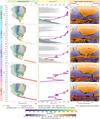 |
Fig. 1 T–p profiles (first column), convective and advective Kzz profiles (second column), and overturning circulation depicted by the mass stream-function Ψ′ (third column) for each simulation. The coloured lines indicate vertical profiles along the equator and the colourbar indicate its coordinates. The dark grey lines show the T–p profiles at latitudes 87°N and 87°S. The bold coloured lines represent profiles at the western and eastern terminators, and sub-stellar and anti-stellar points. The lighter grey lines represent all other vertical profiles. The shaded area indicates the adiabatic regions. The red and magenta shaded area represent the shallowest adiabatic RCB profiles respectively along the equator. The points in column 1 and the horizontal lines in Column 3 show the lowest pressure of the near-adiabatic lines. The purple line in Column 2 shows the absolute advective |Kzz| according Equation (1). The stream-function shows anti-clockwise and clockwise circulations in orange and in purple, respectively. |
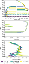 |
Fig. 2 Vertical heat flow ⟨Qr/dt⟩h in the first row (upward heat flow is positive); horizontally averaged Miles instability condition profiles ⟨Ri < Ric⟩h in the second row; and horizontally averaged absolute vertical turbulent heat flux −⟨Feddy⟩h in the third row. The coloured lines indicate the simulations with different Tint. The horizontal lines in the top figure show the lowest pressure of the near-adiabatic lines. The dotted and dash-dotted lines in the top figure respectively indicate the equatorial RCBs and the shallowest RCB for the related Tint. The solid, dashed, and dotted lines indicate Ric with 0.25, 1, and 10, respectively. The dashed and solid lines indicate the −⟨Feddy⟩h calculated with the advective and the total Kzz, respectively. |
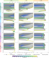 |
Fig. 3 qv (first column), qs (second column), and qc profiles (third column) for each simulation. The coloured lines indicate T–p profiles along the equator and the colourbar indicate its coordinates. The dark grey lines show T–p profiles at the latitudes 87°N and 87°S. The bold coloured lines represent T–p profiles at the western and eastern terminators, and the sub-stellar and anti-stellar points. The lighter grey lines represents all other T–p profiles. |
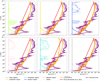 |
Fig. 4 Average Kzz-p profiles of the western region (x > 225° and x < 315°), sub-stellar region (x ≥ −45° and x ≤ 45°), eastern region (x > 45° and x < 135°), global anti-stellar region (x ≥ 45° and x ≤ 135°), and polar region (y ≥ 66.565° or y ≤ 66.565°). For comparison, the common estimate of Kzz in the literature (Lewis et al. 2010; Moses et al. 2011) as |
![Mathematical equation: $\[K_{z z}=H(z) \sqrt{\left\langle w^2\right\rangle_h}\]$](/articles/aa/full_html/2024/11/aa51823-24/aa51823-24-eq5.png)
![Mathematical equation: $\[K_{z z}=5 \cdot 10^4 \sqrt{\frac{p}{10^5}}\]$](/articles/aa/full_html/2024/11/aa51823-24/aa51823-24-eq6.png)
3.2 Post-processing
In this section, we use the 3D spectral radiative transfer model GPU accelerated Cloudy Monte Carlo Radiative Transfer Method (gCMCRT; Lee et al. 2022) on a spherical geometry grid to post-process the GCM results. We examine the effects of changing the internal temperature and cloud structures on the resulting transmission spectra, emission spectra and phase curves of the model output.
Figure 7 presents the transmission spectra of each of the GCM simulations at different Tint. We post-processed the outputs of the simulation with and without the cloud opacities. Higher Tint models lead to a larger transmission (Rp/Rs)2, as previously expected. Additionally, the spectra calculated with cloud opacities lead to larger transmission (Rp/Rs)2 than without cloud opacities. The smaller transmission (Rp/Rs)2 calculated with cloud opacities are due to the high clouds seen on the night-side and in the dusk regions in the GCM simulation. These high clouds extincted stellar flux in layers permeable for stellar light if clouds were absent. The similar offset between all spectra calculated with and without cloud opacities suggest a similar average temperature for the cases with different Tint. The similar temperature on the dayside and the few regions with varying temperatures at low pressure may lead to similar heights.
For the spectrally integrated phase curve, more consequences of the different cloud and temperature structures are revealed in different offsets of the minima in the phase curve (see Fig. 7, top right panel). The absence of cloud opacities lead to a higher emission flux due to the contributions from deeper layers, especially for the emission from the nightside where high clouds could extinct significant more flux of the planetary emission. Interestingly, the most fluxes are extincted in the second-coldest case, which was not expected. However, the coldest case has thinner top clouds and a slightly warmer nightside. A similar feature happens in the warmest cases. The second-warmest case has the least cloud cover on the nightside in the upper atmosphere (pressures p < 104 Pa) based on the GCM simulation. This leads to the highest emissions from the nightside compared to the other cases, although it would radiate less without cloud opacities.
The planetary spectral flux from the dayside does not differ much since the emission comes mostly from cloud-free layers (see Fig. 7, middle left panel). Therefore, the fluxes calculated without cloud opacities do not surpass the other fluxes at most wavelengths. Where they do surpass, the fluxes come from deeper layers. The corresponding brightness temperature at these wavelengths of ~2600 K (see Fig. 7, bottom left panel) linked with the T–p profile (see Figure 1) indicate that some fluxes come from layers with pressures 105 ≲ p ≲ 106 Pa. At these depths, the warmest case has the least cloud cover along the equator. Therefore, the warmest case radiates the most at this wavelength from these layers. Nevertheless, much of these fluxes get extincted by the vapour. At many wavelengths, the coldest case emits the most on the nightside, but the least on the dayside.
On the nightside, clouds reduce significant fluxes at several wavelength ranges (see Fig. 7, middle right panel) compared to the potential fluxes calculated without cloud opacities. The potential fluxes scale hierarchically with Tint throughout the most wavelength ranges with absorption by cloud particles, except for two main wavelength ranges in the near-IR. These two ranges corresponds to a brightness temperature of ~1500 K (see Fig. 7, bottom right panel). This low brightness temperature suggests that emissions from layers lie around the gyres where the two coldest cases are warmer and have top thinner clouds. Inside the gyres (at the lowest brightness temperatures), the potential fluxes are in the warmer cases due to emission from much deeper and warmer layers. Nevertheless, clouds block the emission from the lower layers and only emission from the top layers of the gyres can escape. The gyres of the coldest cases are warmer at the top layers due to a stronger overturning circulation and thereby emit more. Thus, the probed nightside thermal inversion is more pronounced in the colder cases, especially around the gyres. Around the equator’s nightside, the second-warmest case shows the lowest cloud thickness in the upper atmosphere (at pressures p < 104 Pa, see Figure 3). This low cloud thickness allows emissions from deeper layers than in other cases, which we see in the effective fluxes. The corresponding brightness temperatures lie between ~1200 and 1500 K, which matches the temperature in the uppermost equatorial layers on the nightside in the second-warmest case. In the same wavelengths, the warmer cases mostly emit more than the colder cases. Moreover, the warmer cases reduce the emitted fluxes by not very much, as the colder cases do at wavelengths with potentially higher cloud opacities. Thus, the warmer cases smooth the curve of the emission fluxes at the most wavelengths with the most extinction by clouds.
This effect of cloud opacities on the post-processing surpasses the effect of Tint on the nightside. Regarding the wavelength, the effect of cloud opacities on the nightside unfolds mainly in the visible and in some ranges of the near infrared. Therefore, the brightness temperature is higher in these wavelengths. Higher Tint flattens the curves of the planetary spectral flux and brightness temperature for the post-processing with cloud opacities in some ranges in the near-IR bands on the nightside.
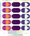 |
Fig. 5 Maps of the temperature in column 1, convective diffusion coefficient Kzz in column 2, and cloud tracer qc in column 3 at pressure surface p = 104 Pa. Each row shows the simulation outputs with different Tint values. The arrows indicate horizontal wind speed and direction. |
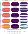 |
Fig. 6 Maps of the temperature in column 1, convective diffusion coefficient Kzz in column 2, and cloud tracer qc in column 3 at pressure surface p = 106 Pa. Each row shows the simulation outputs with different Tint values. The arrows indicate horizontal wind speed and direction. |
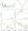 |
Fig. 7 Transmission spectra (top left), phase curves (top right), planetary spectral flux at a longitudinal viewing angle of 15° (center left) and 195° (center right), and brightness temperature at a longitudinal viewing angle of 15° (lower left) and 195° (lower right) based on the post-processing of the GCM simulations. The line styles denote post-processing with (solid) and without (dashed) cloud opacity. |
4 Discussion
In this section, we discuss our results in the context of other studies that investigate vertical mixing and cloud patterns in HJ and UHJ atmospheres.
4.1 Convective inhibition and RCB
As our warmest cases have evolved a near-adiabatic region in the deep atmosphere, convective activities are expected. However, convection seems to be inhibited or the steady-state (warming to the deep adiabat) has not been reached yet. Inhibited convection could be caused by the advection of potential temperature and the turbulent kinetic transport of energy, which we see is significantly stronger in the two warmest cases. Similarly, Guillot & Showman (2002) and Youdin & Mitchell (2010) suggested that convective inhibition can occur by the turbulent kinetic transport of energy (called the mechanical greenhouse effect). All our cases show a burial of heat by a net downward heat advection by atmospheric circulation and waves, as in Showman & Guillot (2002), Guillot & Showman (2002), Tremblin et al. (2017), Sainsbury-Martinez et al. (2019), Mendonça (2020), and Sainsbury-Martinez et al. (2023). We find a global overturning circulation pattern in the upper atmosphere similar to that found in Sainsbury-Martinez et al. (2023), which drives upward vertical and downward transport on the dayside and on the nightside, respectively.
There are other mechanisms of transferring energy to the interior in UHJ such as ohmic heating (Batygin & Stevenson 2010; Perna et al. 2012; Batygin et al. 2011; Huang & Cumming 2012; Rauscher & Menou 2013; Wu & Lithwick 2013; Rogers & Komacek 2014), and atmospheric thermal tides in asynchronous HJ and UHJ (Arras & Socrates 2010; Gu et al. 2019), but these mechanisms are not modelled in the current simulations.
Altering Tint varies the overturning circulation cells and leads to different heat flow and temperature structure. These results are in line with the results in Komacek et al. (2022a). Moreover, these effects couple with opacity inhomogeneities, which alters the temperature structure further, as in Zhang (2023a), Zhang (2023b), and Zhang et al. (2023). They showed that opacity inhomogeneity result in larger cooling of the interior and different pressures of RCB. The combination of the overturning circulation, heat flow, opacity inhomogeneities, and altered Tint lead to large variations in the temperature structure and pressures of RCB in our cases. Consequently, the cloud structure responds to this combined effects. For instance, the pressure of the RCB varies significantly along the latitude and remains homogeneous along the equator, as in Zhang et al. (2023). Their weak drag shows the shallowest RCB in the mid-latitudes, as in our warmest cases. As predicted by Thorngren et al. (2019), higher Tint pushes the RCB to lower pressures in our study.
Our colder cases have not evolved deep or near-adiatbatic thermal profiles. Possible reasons for this lack can be due to a missing steady-state in the deep atmosphere, as in Sainsbury-Martinez et al. (2023), who found a radius inflation up to 50000 simulation days, or that the RCBs of our colder cases actually lie beyond our simulated boundary pressure. The latter is reasonable since the pressure of the RCB increases exponentially the lower the set Tint. As the RCB lies beyond the model boundary, the energy fluxes interact with the lower boundary in the colder cases where the convection in the deep atmosphere is triggered. Additionally, the gradient of the potential temperature in the deep atmosphere gets smaller when the Tint is set lower. Therefore, the deep layers become less stable the lower the Tint is set and more vulnerable to disturbances such as waves and warming. However, longer simulation times may change our results.
4.2 Vertical mixing from convection vs advection
In all our simulations, the global atmosphere generally shows very weak mixing due to convective motions. This is expected from previous theoretical studies (e.g. Parmentier et al. 2013), due to strong irradiation inhibiting convection. However, our simulations show that isolated regions, in particular the nightside Rossby gyres can exhibit strong convective vertical mixing at upper and middle atmospheric regions on par with the advective component.
Modelling and theoretical studies have investigated mixing processes in the atmosphere (e.g. Lewis et al. 2010, Moses et al. 2011, and Parmentier et al. 2013); however, these studies mostly investigated the role of advective mixing, generally ignoring the sub-scale convective component. In Figure 4, we compare commonly used expression of the advective Kzz-profile from the literature to our derived advective and convective Kzz-profile from the GCM simulation. Our simulations produce a partially similar magnitude offset between the Kzz value derived from Equation (2) (Moses et al. 2011; Lewis et al. 2010) and Equation (3) (Parmentier et al. 2013) as noted in Parmentier et al. (2013), but in the upper atmosphere (p ≲ 104 Pa), our advective Kzz exceed the Kzz values derived according to these studies, by up to three magnitudes in some regions. At higher pressures, our advective Kzz lie partially below and above the other Kzz from the literature. This suggests that the Kzz-profiles derived from Equation (2) may be over- or underestimated in Figure 4 for UHJs depending on the pressure. The 1D fit of Kzz in Parmentier et al. (2013) shows that it is made for a specific HJ. Despite this, it is clear from Figure 4 that connvective mixing is magnitudes smaller in the atmosphere. Only very deep regions, p > 107 Pa, show convective mixing that is consistently higher than advective mixing.
The MLT scheme used in our study provides an estimate of the convective strength and estimation of the eddy diffusion coefficient. Our study suggests that there is strong static stability and low convective fluxes in UHJs with warm interiors. Instead, for the colder interior temperatures, convective adjustment is triggered more often and stronger, suggesting that less static stability and higher convective fluxes are required to adjust the atmosphere compared to the hotter interiors. Our results also suggest that warmer interior atmospheres contribute a stabilising effect on the upper atmosphere, reducing the likelihood of upper atmospheric regions undergoing convective adjustment.
Following our results, we suggest that models requiring mixing processes from the deep atmosphere include a convective component when constructing vertical Kzz-profiles. In the upper atmosphere, higher Kzz may appear in isolated regions around and inside the Rossby gyres on the nightside. Rossby gyres play an important role in the non-equilibrium chemical structures of hot Jupiters, where they show strong differences in composition compared to other regions of the atmosphere, such as the equatorial jet (Drummond et al. 2020; Zamyatina et al. 2024). Hence, we suggest including, for GCMs of hot Jupiters, a convective mixing scheme to capture this additional mixing component in the Rossby gyres.
4.3 Cloud structure
Komacek et al. (2022b) performed a tracer-based equilibrium cloud formation model for a UHJ with Tirr = 3348.85 K and Tint = 507 K similar to our study. Their model used the Kzz approach of Parmentier et al. (2013). For the non-radiatively active cloud-case in Komacek et al. (2022b), they predict a cloud base at pressure a bit smaller than 1 · 105 Pa for the equatorial nightside and another cloud base at about 1 · 105 Pa for high latitudinal regions on the nightside. These results disagree with the equatorial cloud base at about 1 · 104 Pa in our simulation and with our cloud base for the high latitudes at around 1 · 106 Pa. The differences in the cloud base may arise from a different temperature structure as our simulations tend to be warmer along the equator and colder at high latitudes in the deep atmosphere. The altered temperature structure is mainly generated by the different radiative transfer scheme (double grey in their model) and the different dynamical core. Additionally, we used other cloud parametrisations (σ = 1 compared to 2, r0 = [2,5] μm compared to rm = 1 μm), which leads to different equilibrium saturation volume mixing ratios, and thereby different cloud structures. Above, their cloud tops lay at pressures of around 1 · 103 Pa for the anti-stellar point and around 1 · 102 Pa for the western terminator; instead, our cloud tops lay beyond the model boundary. The higher cloud fractions around the western terminator and the anti-stellar region in our simulation likely come from lower local temperatures. These lower temperatures are due to the lower set Tirr, the different radiative transfer scheme, and the missing chemical heating effects from hydrogen dissociation and recombination. Moreover, they predict patchy clouds throughout the vertical cloud extent, which in our simulations we only see in the upper cloud layers. Similarly to Komacek et al. (2022b), we see higher emitted nightside flux in a cloud-free atmosphere than in a cloudy atmosphere over a wide range of wavelengths in the gCMCRT post-processing; however, their phase curves show an offset of the hotspot, whereas our phase curves have no offset. The mismatch is likely due to the mentioned warmer temperatures and the resulting shorter radiative timescales in our simulated upper atmospheres.
Roman et al. (2021) and Malsky et al. (2024) studied the impact of vertical mixing through the use of different parametrised vertical cloud extends. They used the RM-GCM with a double-grey two-stream radiative transfer scheme in Roman et al. (2021) and Malsky et al. (2024); a picket fence scheme was also used in Malsky et al. (2024), similar to our study. Additionally, they included radiatively active clouds that condense when the local temperature drops below the condensation temperature of each species. When condensation occurs, they set an immediate change to a condensate with a fraction of 10% in Roman et al. (2021) and Malsky et al. (2024), and to 100% in Roman et al. (2021) of the condensible species. They assumed the abundance of the species to be constant and uniform throughout the atmosphere. For varying strength of the vertical mixing, they implement a pressure-dependent vertical gradient for particle sizes with larger particles at higher pressures. In order to invest different vertical cloud extends, they limit the clouds by force to a smaller vertical extent in the compact case, and set no limit for their extended case. Comparing the vertical cloud extent, our cases with warmer interiors agree more with the extended cases of HD 209458b in Malsky et al. (2024) than to their compact cloud cases. Both of their extended cases show clouds reaching the upper boundary at 1 Pa and a cloud-free day-side, which is in line with our cases. However, the dayside is less cloud-free in both their cases, and their double-grey scheme generates thinner clouds along the equator in the upper atmosphere. Similarly, we see slightly thinner clouds along the upper equator region in our warmer cases. The difference between their RT cases might not only arise from the varied RT schemes, but also from their dual cloud fraction mode (0 or 10% condensed vapour). Comparing the cloud bases, the bases in Malsky et al. (2024) lie globally around 2 · 106 Pa for all their cases of HD 209458b. These pressure heights of the cloud bases agree only with our cases with colder interiors. Moreover, there is a less densely cloudy and cloud-free equator at pressures between ~1 · 104 and ~5 · 105 Pa, respectively, in their picket fence and compact cloud case. This pattern agrees with the cloud structure in our colder and warmer cases at similar pressures. The differences in pressure of cloud bases can arise from from the radiative active clouds, the differently set lower boundary, the multiple cloud species, and the lower temperature in the interior. Compared to Roman et al. (2021), the cloud cover in our study shows similarities to the cloud optical depth (up to 2.8 · 104 Pa) in the 100% condensed-cloud case (for the trend in the simulations between Tirr = 2500 and 3500 K). The densest Al2O3 clouds are at high latitudes on the nightside, and the dayside is cloud-free as in our simulations. The cloud-free dayside is less deformed in their cases, which might be due to weaker winds resulting from a weaker dayside-nightside temperature contrast due to radiatively active clouds and different RT schemes. Equivalent similarities can be seen between the trends in their extended-clouds cases, nucleation-limited-clouds cases, and our cases. However, we see fewer similarities to all their compact cases as the nightside features weaker high latitudinal clouds. As Roman et al. (2021) demonstrated the trend in the offsets of hotspots with increasing Tirr, we show the trend in the eastward offset of the coldspot with increasing Tint (see Figure 7), but the modelled range of Tint leads to no significant offset of the hotspot.
Next, we compared our results to the outcomes of the micro-physical cloud scheme by Powell et al. (2018). They find a similar trend in the increase in the vertical extent of TiO2 and MgSiO3 clouds in HJs when setting a deep cold trap. This cold trap leads to the formation of a second cloud population in the deep atmosphere depending on the cloud particle size. The two cloud populations extend vertically and get connected when they set lower equilibrium temperatures, but at higher equilibrium temperatures the deep cloud population gets vertically smaller and starts to disappear. We also see such a deep cloud population (1 · 106 < p < 1 · 108 Pa) in our colder cases. However, microphysical processes, vertical mixing, and settling change the cloud particle sizes, as shown in their study. They predicted bimodal or irregular shapes in the cloud particle size distribution, which lead to more complex cloud structures. These implications on the cloud particle distribution would probably change our results significantly. For instance, our colder cases may underestimate the efficiency of the deep cold trap due to inappropriate cloud particle distributions, which may lead to too much and too high cloud formation in the upper atmosphere. Nonetheless, our results agree with those of Powell et al. (2018) that deep cold traps still allow significant cloud formation in the upper atmosphere.
4.4 Limitations and future improvements
Our study focuses on and isolates the effect of the Tint and mixing on the cloud structure. Therefore, we do not include radiatively active clouds as Roman et al. (2021), Komacek et al. (2022b), and Malsky et al. (2024) do, although they showed that clouds change the temperature structure and atmospheric dynamics. Firstly, such radiatively active clouds lead to an increase in the scattering at short wavelengths by high-altitude dayside clouds, increases the albedo, and thereby lowers the temperature of the planet (Parmentier et al. 2016). Secondly, radiatively active clouds increase the scattering and absorption in the thermal wavelengths, which results in a greenhouse effect below the clouds. Additionally, including heat exchange from H2 dissociation and recombination lead to a reduced day-night temperature contrast (Tan & Komacek 2019). Further, we implemented a tracer-based equilibrium cloud model, which is simpler than the more sophisticated microphysical cloud scheme with an appropriate cloud particle size distributions by Powell et al. (2018). Implementing a cloud scheme that considers the locally unique cloud particle size distribution in cloud formation processes may change the outcome of our study. Furthermore, longer simulation runs of up to 50000 days, as in Sainsbury-Martinez et al. (2023), may evolve altered temperature structures and altered overturning circulations that affect the cloud structure. Finally, using a different set of hydrodynamic equations may change the jet structure and overturning circulation in our results significantly (Mayne et al. 2019; Deitrick et al. 2020; Noti et al. 2023).
5 Conclusions
Convection is inhibited in hot-Jupiter atmospheres above the radiative-convective boundary due to their strong irradiation. We demonstrated that ultra-hot Jupiters (UHJs) with warm interiors have strong static stability and low convective fluxes. Therefore, the advective component is more dominant in shaping the cloud structure in UHJs with warm interiors than the convective mixing. To the contrary, we see that UHJs with colder interiors show less static stability, which lead to more convective adjustment and higher convective fluxes than those with hotter interiors. Stronger cooling of the interior is expected in the UHJs with colder interiors, due to opacity inhomogeneities and convection. Ultra-hot Jupiters with warmer interiors have higher vertical turbulent heat fluxes. In combination with the vertical advection of potential temperature (altered circulation cells) and weaker cooling due to higher opacities in the deep atmosphere, the turbulent heat fluxes inhibit convection in the deep atmosphere in the warmer cases. As a consequence of the lower temperatures and increased convective mixing, a global cloud layer forms in the deepest inversion in the cooler cases. Therefore, the vertical extent of the cloud structures are increased as the internal temperature is decreased. Our results show that vertical convective mixing becomes consistently higher than advective mixing in cold interiors of highly irradiated gas giants. In addition, strong vertical convective mixing may occur in isolated regions around and inside the Rossby gyres on the nightside. Therefore, we suggest models that include a vertical convective mixing scheme that quantifies additional mixing in the Rossby gyres more adequately. Overall, convective mixing globally plays a minor role in keeping cloud particles aloft in UHJs.
Future investigations may extend this study by adding radiatively active clouds as in Roman et al. (2021), Komacek et al. (2022b), and Malsky et al. (2024). Moreover, this study can be continued by including multiple cloud species, as in (Roman et al. 2021) and Malsky et al. (2024). Alternatively, a microphysical cloud scheme such as CARMA (Gao et al. 2018; Powell et al. 2018) could be coupled to the GCM.
Data availability
The 1D radiative-transfer, gCMCRT and various other source codes are available on GitHub: https://github.com/ELeeAstro. The input of the Exo-FMS GCM and the post-processings with gCMCRT are available on Zenodo, at https://doi.org/10.5281/zenodo.13254749. All other data and code are available from the authors on a collaborative basis. All other data are available upon request to the lead author.
Acknowledgements
P. Noti and E.K.H. Lee are supported by the SNSF Ambizione Fellowship grant (#193448), a scheme of the Swiss National Science Foundation. Calculations were performed on UBELIX (http://www.id.unibe.ch/hpc), the HPC cluster at the University of Bern. We thank the IT Service Office (Ubelix cluster), the Physikalisches Institut and the Center for Space and Habitability at the Universität of Bern for their services. Data and plots were processed and produced using PYTHON version 3.9 (Van Rossum & Drake Jr 1995) and the community open-source PYTHON packages Bokeh (Bokeh Development Team 2022), Matplotlib (Hunter 2007), cartopy (Met Office 2010–2015; Elson et al. 2022), jupyter (Kluyver et al. 2016), NumPy (Harris et al. 2020), pandas (pandas development team 2020), SciPy (Jones et al. 2001), seaborn (Waskom 2021), windspharm (Dawson 2016) and xarray Hoyer & Hamman (2017). Parts of this work have been carried out within the framework of the NCCR PlanetS supported by the Swiss National Science Foundation under grants 51NF40_182901 and 51NF40_205606.
Appendix A Vertical heat flow
For quantifying the advection of potential temperature, we follow a similar approach as in Sainsbury-Martinez et al. (2023). The mean vertical enthalpy advection FHr [Wm−2] can be quantified as in Sainsbury-Martinez et al. (2023) as
![Mathematical equation: $\[F_{\mathcal{H} r}=\rho c_p T w,\]$](/articles/aa/full_html/2024/11/aa51823-24/aa51823-24-eq7.png) (A.1)
(A.1)
where ρ [kgm−3] is the density of the gas, cp [Jkg−1K−1] stands for the specific heat capacity, and w [ms−1] denotes the vertical wind speed. In order to address varying grid point sizes, we take the surface integral of mean vertical enthalpy advection so that Equation A.1 becomes
![Mathematical equation: $\[\frac{Q_r}{\partial t}=\int_0^{2 \pi} \int_0^{2 \pi} \rho c_p T ~w R^2 ~\cos ~\phi~ d \phi ~d \lambda,\]$](/articles/aa/full_html/2024/11/aa51823-24/aa51823-24-eq8.png) (A.2)
(A.2)
where ϕ and λ are the latitudinal and longitudinal angles, and R [m] stands for the distance from the planetary center to the specific pressure surface. R has the relation R = rp + z, where rp [m] is the radius of reference surface and z [m] the height from the reference surface to the specific pressure surface. As most planets have rp ≫ z, we ignore z.
Appendix B The Richardson number
Many studies rely on Miles instability condition if the Richardson number is lower than the critical value Rig < Ric (Miles 1961; Abarbanel et al. 1984, Ric between 0.25 and 1) to estimate the stability of the flow and the presence of turbulence (see Egerer et al. 2023; Ostrovsky et al. 2024). The gradient Richardson number Rig describes the ratio of the buoyancy N [s−1] (the Brunt-Väisälä frequency) to the wind shear S [s−1] as
![Mathematical equation: $\[R i_g=\frac{N^2}{S^2}=\frac{g}{T_v} \frac{\frac{\partial \theta_v}{\partial z}}{\left(\frac{\partial v_h}{\partial z}\right)^2},\]$](/articles/aa/full_html/2024/11/aa51823-24/aa51823-24-eq9.png) (B.1)
(B.1)
where g [1 ms−2] is the gravity, Tv [K] represents the virtual temperature, θν [K] stands for the virtual potential temperature, z [m] denotes the height, and vh [ms−1] is the horizontal velocity. The Ric has been altered in several ocean and atmospheric studies (see Egerer et al. 2023). Recent observations revealed that turbulence even occur at Rig up to 10 and more (Ostrovsky et al. 2024, see). Nevertheless, low Rig still indicates the presence of turbulent flow. In this study, we made use of 3 thresholds for Ric = 0.25, 1 or 10 as different uncertainty thresholds.
Appendix C Turbulent heat flux
For quantifying the turbulent heat transfer, we follow Youdin & Mitchell (2010). They expressed the turbulent heat flux Feddy [Wm−2] as
![Mathematical equation: $\[F_{e d d y}=-K_{z z} \rho g\left(1-\frac{\nabla}{\nabla_{a d}}\right),\]$](/articles/aa/full_html/2024/11/aa51823-24/aa51823-24-eq10.png) (C.1)
(C.1)
where Kzz [m2 s−1] denotes the (thermal) eddy diffusion coefficient, ρ [kgm−3] is the density of the gas, g [1 ms−2] represents the gravity, ∇ [K] is the vertical lapse rate (temperature gradient), and ∇ad [K] denotes the adiabatic lapse rate.
References
- Abarbanel, H. D. I., Holm, D. D., Marsden, J. E., & Ratiu, T. 1984, Phys. Rev. Lett., 52, 2352 [CrossRef] [Google Scholar]
- Ackerman, A. S., & Marley, M. S. 2001, ApJ, 556, 872 [Google Scholar]
- Andrews, D. G., Holton, J. R., & Leovy, C. B. 1987, Middle Atmosphere Dynamics [Google Scholar]
- Arcangeli, J., Désert, J.-M., Parmentier, V., et al. 2019, A&A, 625, A136 [NASA ADS] [CrossRef] [EDP Sciences] [Google Scholar]
- Arras, P., & Socrates, A. 2010, ApJ, 714, 1 [Google Scholar]
- Batygin, K., & Stevenson, D. J. 2010, ApJ, 714, L238 [NASA ADS] [CrossRef] [Google Scholar]
- Batygin, K., Stevenson, D. J., & Bodenheimer, P. H. 2011, ApJ, 738, 1 [NASA ADS] [CrossRef] [Google Scholar]
- Bokeh Development Team. 2022, Bokeh: Python Library for Interactive Visualization [Google Scholar]
- Bourrier, V., Kitzmann, D., Kuntzer, T., et al. 2020, A&A, 637, A36 [NASA ADS] [CrossRef] [EDP Sciences] [Google Scholar]
- Brogi, M., Emeka-Okafor, V., Line, M. R., et al. 2023, AJ, 165, 91 [NASA ADS] [CrossRef] [Google Scholar]
- Chamberlain, J. W., & Hunten, D. M. 1987, Theory of Planetary Atmospheres. An Introduction to their Physics Andchemistry, 36 (Academic Press) [Google Scholar]
- Christiansen, J. L., Ballard, S., Charbonneau, D., et al. 2010, ApJ, 710, 97 [NASA ADS] [CrossRef] [Google Scholar]
- Cooper, C. S., & Showman, A. P. 2006, ApJ, 649, 1048 [CrossRef] [Google Scholar]
- Coulombe, L.-P., Benneke, B., Challener, R., et al. 2023, Nature, 620, 292 [NASA ADS] [CrossRef] [Google Scholar]
- Dawson, A. 2016, J. Open Res. Softw., 4, 1 [CrossRef] [Google Scholar]
- Daylan, T., Günther, M. N., Mikal-Evans, T., et al. 2021, AJ, 161, 131 [NASA ADS] [CrossRef] [Google Scholar]
- Deitrick, R., Mendonça, J. M., Schroffenegger, U., et al. 2020, ApJS, 248, 30 [NASA ADS] [CrossRef] [Google Scholar]
- Deitrick, R., Heng, K., Schroffenegger, U., et al. 2022, MNRAS, 512, 3759 [NASA ADS] [CrossRef] [Google Scholar]
- Delrez, L., Santerne, A., Almenara, J. M., et al. 2016, MNRAS, 458, 4025 [NASA ADS] [CrossRef] [Google Scholar]
- Doyon, R., Hutchings, J. B., Beaulieu, M., et al. 2012, SPIE Conf. Ser., 8442, 84422R [NASA ADS] [Google Scholar]
- Drummond, B., Hébrard, E., Mayne, N. J., et al. 2020, A&A, 636, A68 [NASA ADS] [CrossRef] [EDP Sciences] [Google Scholar]
- Egerer, U., Cassano, J. J., Shupe, M. D., et al. 2023, Atmos. Meas. Tech., 16, 2297 [NASA ADS] [CrossRef] [Google Scholar]
- Elson, P., de Andrade, E. S., Lucas, G., et al. 2022, https://doi.org/10.5281/zenodo.7430317 [Google Scholar]
- Evans, T. M., Sing, D. K., Wakeford, H. R., et al. 2016, ApJ, 822, L4 [NASA ADS] [CrossRef] [Google Scholar]
- Evans, T. M., Sing, D. K., Goyal, J. M., et al. 2018, AJ, 156, 283 [NASA ADS] [CrossRef] [Google Scholar]
- Fu, G., Deming, D., Lothringer, J., et al. 2021, AJ, 162, 108 [NASA ADS] [CrossRef] [Google Scholar]
- Gandhi, S., Landman, R., Snellen, I., et al. 2024, MNRAS, 530, 2885 [NASA ADS] [CrossRef] [Google Scholar]
- Gao, P., Marley, M. S., & Ackerman, A. S. 2018, ApJ, 855, 86 [Google Scholar]
- Gibson, N. P., Merritt, S., Nugroho, S. K., et al. 2020, MNRAS, 493, 2215 [Google Scholar]
- Gu, P.-G., Peng, D.-K., & Yen, C.-C. 2019, ApJ, 887, 228 [NASA ADS] [CrossRef] [Google Scholar]
- Guillot, T., Burrows, A., Hubbard, W. B., Lunine, J. I., & Saumon, D. 1996, ApJ, 459, L35 [Google Scholar]
- Guillot, T., & Showman, A. P. 2002, A&A, 385, 156 [NASA ADS] [CrossRef] [EDP Sciences] [Google Scholar]
- Harris, C. R., Millman, K. J., van der Walt, S. J., et al. 2020, Nature, 585, 357 [NASA ADS] [CrossRef] [Google Scholar]
- Helling, C. 2019, Annu. Rev. Earth Planet. Sci., 47, 583 [CrossRef] [Google Scholar]
- Heng, K., Frierson, D. M. W., & Phillipps, P. J. 2011, MNRAS, 418, 2669 [NASA ADS] [CrossRef] [Google Scholar]
- Hoeijmakers, H. J., Seidel, J. V., Pino, L., et al. 2020, A&A, 641, A123 [NASA ADS] [CrossRef] [EDP Sciences] [Google Scholar]
- Hoyer, S., & Hamman, J. 2017, J. Open Research Softw., 5, 1 [Google Scholar]
- Huang, X., & Cumming, A. 2012, ApJ, 757, 47 [NASA ADS] [CrossRef] [Google Scholar]
- Hunter, J. D. 2007, Comput. Sci. Eng., 9, 90 [NASA ADS] [CrossRef] [Google Scholar]
- Jones, E., Oliphant, T., Peterson, P., et al. 2001, SciPy: Open source scientific tools for Python [Google Scholar]
- Joyce, M., & Tayar, J. 2023, Galaxies, 11, 75 [NASA ADS] [CrossRef] [Google Scholar]
- Kluyver, T., Ragan-Kelley, B., Pérez, F., et al. 2016, in IOS Press (IOS Press Ebooks), 87 [Google Scholar]
- Komacek, T. D., Gao, P., Thorngren, D. P., May, E. M., & Tan, X. 2022a, ApJ, 941, L40 [NASA ADS] [CrossRef] [Google Scholar]
- Komacek, T. D., Tan, X., Gao, P., & Lee, E. K. H. 2022b, ApJ, 934, 79 [NASA ADS] [CrossRef] [Google Scholar]
- Lafreniere, D. 2017, NIRISS Exploration of the Atmospheric diversity of Transiting exoplanets (NEAT), JWST Proposal. Cycle 1, ID #1201 [Google Scholar]
- Lafreniere, D. 2022, NIRISS Exploration of the Atmospheric diversity of Transiting exoplanets (NEAT), JWST Proposal. Cycle 2, ID #2759 [Google Scholar]
- Landman, R., Sánchez-López, A., Mollière, P., et al. 2021, A&A, 656, A119 [NASA ADS] [CrossRef] [EDP Sciences] [Google Scholar]
- Lee, E. K. H., Parmentier, V., Hammond, M., et al. 2021, MNRAS, 506, 2695 [NASA ADS] [CrossRef] [Google Scholar]
- Lee, E. K. H., Prinoth, B., Kitzmann, D., et al. 2022, MNRAS, 517, 240 [NASA ADS] [CrossRef] [Google Scholar]
- Lee, E. K. H., Tan, X., & Tsai, S.-M. 2024, MNRAS, 529, 2686 [NASA ADS] [CrossRef] [Google Scholar]
- Lewis, N. K., Showman, A. P., Fortney, J. J., et al. 2010, ApJ, 720, 344 [NASA ADS] [CrossRef] [Google Scholar]
- Malsky, I., Rauscher, E., Roman, M. T., et al. 2024, ApJ, 961, 66 [NASA ADS] [CrossRef] [Google Scholar]
- Mansfield, M. 2023, Ap&SS, 368, 24 [NASA ADS] [CrossRef] [Google Scholar]
- Mansfield, M., Bean, J. L., Line, M. R., et al. 2018, AJ, 156, 10 [NASA ADS] [CrossRef] [Google Scholar]
- Mansfield, M., Bean, J. L., Stevenson, K. B., et al. 2020, ApJ, 888, L15 [Google Scholar]
- Marley, M. S., & Robinson, T. D. 2015, ARA&A, 53, 279 [Google Scholar]
- Marley, M. S., Gelino, C., Stephens, D., Lunine, J. I., & Freedman, R. 1999, ApJ, 513, 879 [NASA ADS] [CrossRef] [Google Scholar]
- Maxted, P. F. L., Anderson, D. R., Doyle, A. P., et al. 2013, MNRAS, 428, 2645 [NASA ADS] [CrossRef] [Google Scholar]
- Mayne, N. J., Drummond, B., Debras, F., et al. 2019, ApJ, 871, 56 [Google Scholar]
- Mendonça, J. M. 2020, MNRAS, 491, 1456 [CrossRef] [Google Scholar]
- Merritt, S. R., Gibson, N. P., Nugroho, S. K., et al. 2020, A&A, 636, A117 [NASA ADS] [CrossRef] [EDP Sciences] [Google Scholar]
- Merritt, S. R., Gibson, N. P., Nugroho, S. K., et al. 2021, MNRAS, 506, 3853 [NASA ADS] [CrossRef] [Google Scholar]
- Met Office. 2010–2015, Cartopy: a cartographic python library with a Matplotlib interface, Exeter, Devon [Google Scholar]
- Mikal-Evans, T., Sing, D. K., Kataria, T., et al. 2020, MNRAS, 496, 1638 [Google Scholar]
- Mikal-Evans, T., Sing, D. K., Barstow, J. K., et al. 2022, Nat. Astron., 6, 471 [NASA ADS] [CrossRef] [Google Scholar]
- Mikal-Evans, T., Sing, D. K., Dong, J., et al. 2023, ApJ, 943, L17 [CrossRef] [Google Scholar]
- Miles, J. W. 1961, J. Fluid Mech., 10, 496 [Google Scholar]
- Moses, J. I., Visscher, C., Fortney, J. J., et al. 2011, ApJ, 737, 15 [Google Scholar]
- Noti, P. A., Lee, E. K. H., Deitrick, R., & Hammond, M. 2023, MNRAS, 524, 3396 [NASA ADS] [CrossRef] [Google Scholar]
- Ostrovsky, L., Soustova, I., Troitskaya, Y., & Gladskikh, D. 2024, Nonlinear Processes Geophys., 31, 219 [NASA ADS] [CrossRef] [Google Scholar]
- Ouyang, Q., Wang, W., Zhai, M., et al. 2023, Res. Astron. Astrophys., 23, 065010 [CrossRef] [Google Scholar]
- pandas development team, T. 2020, https://doi.org/10.5281/zenodo.3509134 [Google Scholar]
- Parmentier, V., & Guillot, T. 2014, A&A, 562, A133 [NASA ADS] [CrossRef] [EDP Sciences] [Google Scholar]
- Parmentier, V., & Crossfield, I. J. M. 2018, in Handbook of Exoplanets, eds. H. J. Deeg, & J. A. Belmonte (Springer International Publishing AG), 116 [Google Scholar]
- Parmentier, V., Showman, A. P., & Lian, Y. 2013, A&A, 558, A91 [NASA ADS] [CrossRef] [EDP Sciences] [Google Scholar]
- Parmentier, V., Guillot, T., Fortney, J. J., & Marley, M. S. 2015, A&A, 574, A35 [NASA ADS] [CrossRef] [EDP Sciences] [Google Scholar]
- Parmentier, V., Fortney, J. J., Showman, A. P., Morley, C., & Marley, M. S. 2016, ApJ, 828, 22 [Google Scholar]
- Parmentier, V., Line, M. R., Bean, J. L., et al. 2018, A&A, 617, A110 [NASA ADS] [CrossRef] [EDP Sciences] [Google Scholar]
- Perna, R., Heng, K., & Pont, F. 2012, ApJ, 751, 59 [NASA ADS] [CrossRef] [Google Scholar]
- Powell, D., Zhang, X., Gao, P., & Parmentier, V. 2018, ApJ, 860, 18 [Google Scholar]
- Quirrenbach, A., Amado, P. J., Caballero, J. A., et al. 2014, SPIE Conf. Ser., 9147, 91471F [Google Scholar]
- Rauscher, E., & Menou, K. 2013, ApJ, 764, 103 [NASA ADS] [CrossRef] [Google Scholar]
- Rogers, T. M., & Komacek, T. D. 2014, ApJ, 794, 132 [NASA ADS] [CrossRef] [Google Scholar]
- Roman, M. T., Kempton, E. M. R., Rauscher, E., et al. 2021, ApJ, 908, 101 [CrossRef] [Google Scholar]
- Sainsbury-Martinez, F., Wang, P., Fromang, S., et al. 2019, A&A, 632, A114 [NASA ADS] [CrossRef] [EDP Sciences] [Google Scholar]
- Sainsbury-Martinez, F., Tremblin, P., Schneider, A. D., et al. 2023, MNRAS, 524, 1316 [NASA ADS] [CrossRef] [Google Scholar]
- Sarkis, P., Mordasini, C., Henning, T., Marleau, G. D., & Mollière, P. 2021, A&A, 645, A79 [NASA ADS] [CrossRef] [EDP Sciences] [Google Scholar]
- Seager, S., & Sasselov, D. D. 1998, ApJ, 502, L157 [NASA ADS] [CrossRef] [Google Scholar]
- Showman, A. P., & Dowling, T. E. 2000, Science, 289, 1737 [NASA ADS] [Google Scholar]
- Showman, A. P., & Guillot, T. 2002, A&A, 385, 166 [NASA ADS] [CrossRef] [EDP Sciences] [Google Scholar]
- Showman, A. P., Cooper, C. S., Fortney, J. J., & Marley, M. S. 2008, ApJ, 682, 559 [NASA ADS] [CrossRef] [Google Scholar]
- Showman, A. P., Fortney, J. J., Lewis, N. K., & Shabram, M. 2013, ApJ, 762, 24 [Google Scholar]
- Showman, A. P., Fortney, J. J., Lian, Y., et al. 2009, ApJ, 699, 564 [NASA ADS] [CrossRef] [Google Scholar]
- Smith, M. D. 1998, Icarus, 132, 176 [NASA ADS] [CrossRef] [Google Scholar]
- Spiegel, D. S., Silverio, K., & Burrows, A. 2009, ApJ, 699, 1487 [Google Scholar]
- Sudarsky, D., Burrows, A., & Hubeny, I. 2003, ApJ, 588, 1121 [Google Scholar]
- Tan, X., & Komacek, T. D. 2019, ApJ, 886, 26 [Google Scholar]
- Tan, X., & Showman, A. P. 2021a, MNRAS, 502, 678 [NASA ADS] [CrossRef] [Google Scholar]
- Tan, X., & Showman, A. P. 2021b, MNRAS, 502, 2198 [NASA ADS] [CrossRef] [Google Scholar]
- Tan, X., Komacek, T. D., Batalha, N. E., et al. 2024, MNRAS, 528, 1016 [NASA ADS] [CrossRef] [Google Scholar]
- Thorngren, D., Gao, P., & Fortney, J. J. 2019, ApJ, 884, L6 [Google Scholar]
- Tremblin, P., Chabrier, G., Mayne, N. J., et al. 2017, ApJ, 841, 30 [NASA ADS] [CrossRef] [Google Scholar]
- Tsai, S.-M., Lyons, J. R., Grosheintz, L., et al. 2017, ApJS, 228, 20 [NASA ADS] [CrossRef] [Google Scholar]
- Van Rossum, G., & Drake Jr, F. L. 1995, Python Tutorial (The Netherlands: Centrum voor Wiskunde en Informatica Amsterdam) [Google Scholar]
- Waskom, M. 2021, J. Open Source Softw., 6, 3021 [CrossRef] [Google Scholar]
- West, R. G., Hellier, C., Almenara, J. M., et al. 2016, A&A, 585, A126 [NASA ADS] [CrossRef] [EDP Sciences] [Google Scholar]
- Wilson, J., Gibson, N. P., Lothringer, J. D., et al. 2021, MNRAS, 503, 4787 [NASA ADS] [CrossRef] [Google Scholar]
- Woitke, P., & Helling, C. 2004, A&A, 414, 335 [NASA ADS] [CrossRef] [EDP Sciences] [Google Scholar]
- Woitke, P., Helling, C., Hunter, G. H., et al. 2018, A&A, 614, A1 [NASA ADS] [CrossRef] [EDP Sciences] [Google Scholar]
- Wong, I., Knutson, H. A., Kataria, T., et al. 2016, ApJ, 823, 122 [NASA ADS] [CrossRef] [Google Scholar]
- Wu, Y., & Lithwick, Y. 2013, ApJ, 763, 13 [NASA ADS] [CrossRef] [Google Scholar]
- Youdin, A. N., & Mitchell, J. L. 2010, ApJ, 721, 1113 [NASA ADS] [CrossRef] [Google Scholar]
- Zamyatina, M., Christie, D. A., Hébrard, E., et al. 2024, MNRAS, 529, 1776 [NASA ADS] [CrossRef] [Google Scholar]
- Zhang, X. 2023a, ApJ, 957, 20 [NASA ADS] [CrossRef] [Google Scholar]
- Zhang, X. 2023b, ApJ, 957, 21 [CrossRef] [Google Scholar]
- Zhang, X., & Showman, A. P. 2018a, ApJ, 866, 1 [NASA ADS] [CrossRef] [Google Scholar]
- Zhang, X., & Showman, A. P. 2018b, ApJ, 866, 2 [NASA ADS] [CrossRef] [Google Scholar]
- Zhang, X., Li, C., Ge, H., & Le, T. 2023, ApJ, 957, 22 [NASA ADS] [CrossRef] [Google Scholar]
All Tables
Defined parameters for the all GCM simulations using a C32 resolution grid (≈128 × 64 longitude×latitude).
All Figures
|
Fig. 1 T–p profiles (first column), convective and advective Kzz profiles (second column), and overturning circulation depicted by the mass stream-function Ψ′ (third column) for each simulation. The coloured lines indicate vertical profiles along the equator and the colourbar indicate its coordinates. The dark grey lines show the T–p profiles at latitudes 87°N and 87°S. The bold coloured lines represent profiles at the western and eastern terminators, and sub-stellar and anti-stellar points. The lighter grey lines represent all other vertical profiles. The shaded area indicates the adiabatic regions. The red and magenta shaded area represent the shallowest adiabatic RCB profiles respectively along the equator. The points in column 1 and the horizontal lines in Column 3 show the lowest pressure of the near-adiabatic lines. The purple line in Column 2 shows the absolute advective |Kzz| according Equation (1). The stream-function shows anti-clockwise and clockwise circulations in orange and in purple, respectively. |
| In the text | |
|
Fig. 2 Vertical heat flow ⟨Qr/dt⟩h in the first row (upward heat flow is positive); horizontally averaged Miles instability condition profiles ⟨Ri < Ric⟩h in the second row; and horizontally averaged absolute vertical turbulent heat flux −⟨Feddy⟩h in the third row. The coloured lines indicate the simulations with different Tint. The horizontal lines in the top figure show the lowest pressure of the near-adiabatic lines. The dotted and dash-dotted lines in the top figure respectively indicate the equatorial RCBs and the shallowest RCB for the related Tint. The solid, dashed, and dotted lines indicate Ric with 0.25, 1, and 10, respectively. The dashed and solid lines indicate the −⟨Feddy⟩h calculated with the advective and the total Kzz, respectively. |
| In the text | |
|
Fig. 3 qv (first column), qs (second column), and qc profiles (third column) for each simulation. The coloured lines indicate T–p profiles along the equator and the colourbar indicate its coordinates. The dark grey lines show T–p profiles at the latitudes 87°N and 87°S. The bold coloured lines represent T–p profiles at the western and eastern terminators, and the sub-stellar and anti-stellar points. The lighter grey lines represents all other T–p profiles. |
| In the text | |
|
Fig. 4 Average Kzz-p profiles of the western region (x > 225° and x < 315°), sub-stellar region (x ≥ −45° and x ≤ 45°), eastern region (x > 45° and x < 135°), global anti-stellar region (x ≥ 45° and x ≤ 135°), and polar region (y ≥ 66.565° or y ≤ 66.565°). For comparison, the common estimate of Kzz in the literature (Lewis et al. 2010; Moses et al. 2011) as |
| In the text | |
|
Fig. 5 Maps of the temperature in column 1, convective diffusion coefficient Kzz in column 2, and cloud tracer qc in column 3 at pressure surface p = 104 Pa. Each row shows the simulation outputs with different Tint values. The arrows indicate horizontal wind speed and direction. |
| In the text | |
|
Fig. 6 Maps of the temperature in column 1, convective diffusion coefficient Kzz in column 2, and cloud tracer qc in column 3 at pressure surface p = 106 Pa. Each row shows the simulation outputs with different Tint values. The arrows indicate horizontal wind speed and direction. |
| In the text | |
|
Fig. 7 Transmission spectra (top left), phase curves (top right), planetary spectral flux at a longitudinal viewing angle of 15° (center left) and 195° (center right), and brightness temperature at a longitudinal viewing angle of 15° (lower left) and 195° (lower right) based on the post-processing of the GCM simulations. The line styles denote post-processing with (solid) and without (dashed) cloud opacity. |
| In the text | |
Current usage metrics show cumulative count of Article Views (full-text article views including HTML views, PDF and ePub downloads, according to the available data) and Abstracts Views on Vision4Press platform.
Data correspond to usage on the plateform after 2015. The current usage metrics is available 48-96 hours after online publication and is updated daily on week days.
Initial download of the metrics may take a while.