| Issue |
A&A
Volume 691, November 2024
|
|
|---|---|---|
| Article Number | A220 | |
| Number of page(s) | 19 | |
| Section | Stellar atmospheres | |
| DOI | https://doi.org/10.1051/0004-6361/202451173 | |
| Published online | 15 November 2024 | |
Chemical Evolution of R-process Elements in Stars (CERES)
II. The impact of stellar evolution and rotation on light and heavy elements
1
Goethe University Frankfurt, Institute for Applied Physics,
Max-von-Laue-Str. 12,
60438
Frankfurt am Main,
Germany
2
INAF, Osservatorio di Astrofisica e Scienza dello Spazio,
Via Gobetti 93/3,
40129
Bologna,
Italy
3
Department of Astronomy, University of Geneva,
Chemin Pegasi 51,
1290
Versoix,
Switzerland
★ Corresponding author; This email address is being protected from spambots. You need JavaScript enabled to view it.
Received:
19
June
2024
Accepted:
4
September
2024
Abstract
Context. Carbon, nitrogen, and oxygen are the most abundant elements throughout the universe, after hydrogen and helium. Studying these elements in low-metallicity stars can provide crucial information on the chemical composition in the early Galaxy and possible internal mixing processes that can alter the surface composition of the stars.
Aims. This work aims to investigate the chemical abundance patterns for CNO elements and Li in a homogeneously analyzed sample of 52 metal-poor halo giant stars. From these results, we have been able to determine whether internal mixing processes have taken place in these stars.
Methods. We used high-resolution spectra with a high signal-to-noise ratio (S/N) to carry out a spectral synthesis to derive detailed C, N, O, and Li abundances for a sample of stars with metallicities in the range of −3.58 ≤ [Fe/H] ≤ −1.79 dex. Our study was based on the assumption of one-dimensional (1D) local thermodynamic equilibrium (LTE) atmospheres.
Results. Based on carbon and nitrogen abundances, we investigated the deep mixing taking place within stars along the red giant branch (RGB). The individual abundances of carbon decrease towards the upper RGB while nitrogen shows an increasing trend, indicating that carbon has been converted into nitrogen. No signatures of ON-cycle processed material were found for the stars in our sample. We computed a set of galactic chemical evolution (GCE) models, implementing different sets of massive star yields, both with and without including the effects of stellar rotation on nucleosynthesis. We confirm that stellar rotation is necessary to explain the highest [N/Fe] and [N/O] ratios observed in unmixed halo stars. The predicted level of N enhancement varies sensibly in dependence of the specific set of yields that are adopted. For stars with stellar parameters similar to those of our sample, heavy elements such as Sr, Y, and Zr appear to have unchanged abundances despite the stellar evolution mixing processes.
Conclusions. The unmixed RGB stars provide very useful constraints on chemical evolution models of the Galaxy. As they are more luminous than unevolved (main sequence and turnoff) stars, they also allow for stars to be probed at greater distances. The stellar CN-cycle clearly changes the atmospheric abundances of the lighter elements, but no changes were detected with respect to the heavy elements.
Key words: stars: abundances / stars: atmospheres / stars: evolution / stars: Population II / galaxy: halo
© The Authors 2024
 Open Access article, published by EDP Sciences, under the terms of the Creative Commons Attribution License (https://creativecommons.org/licenses/by/4.0), which permits unrestricted use, distribution, and reproduction in any medium, provided the original work is properly cited.
This article is published in open access under the Subscribe to Open model. This email address is being protected from spambots. You need JavaScript enabled to view it. to support open access publication.
1 Introduction
Carbon, nitrogen, and oxygen are among the most abundant elements throughout the Universe. A well-established fact in nuclear astrophysics is that carbon, nitrogen, and oxygen are synthesized through hydrostatic nuclear fusion occurring in different stages of stellar evolution or by explosive burning taking place in the end of the evolution of massive stars (Burbidge et al. 1957; Nomoto et al. 2013; Kobayashi et al. 2020; Romano 2022; Arcones & Thielemann 2023). The nucleosynthetic processes in the stellar interior that lead to the production of these elements are also well known and depend on the mass, metallicity, and rotation of the star, with the role of binary interactions yet to be fully investigated (e.g., Farmer et al. 2021).
The stable isotopes of carbon and oxygen are primarily synthesized by hydrostatic He burning through the triple-α reaction (Hoyle 1954; Woosley et al. 2002). Although carbon is produced in stars of all masses, asymptotic giant branch (AGB) star models estimate a contribution of roughly one third of the 12C found in the Galaxy (Karakas & Lattanzio 2014) This is in agreement with Romano et al. (2020) finding that 60–70% of C being formed by massive stars1. On the other hand, the main contribution to the oxygen abundance comes from massive stars via core-collapse supernovae (CCSNe) (Vincenzo et al. 2016). Oxygen is the most abundant metal in stars. Nitrogen is mainly a secondary element and mostly produced by low- and intermediate-mass stars through the CN-cycle at the expense of the carbon and oxygen initially present in the star. If nuclear burning at the base of the convective envelope is efficient, nitrogen can also be produced as a primary element from the original hydrogen and helium during the third dredge-up (TDU) in AGB stars (Renzini & Voli 1981).
Stellar models have shown that at low metallicities, rotation also has a significant impact on the observed abundance of the CNO elements on the surface of the stars. This is due to the fact that the mixing of chemical elements becomes more efficient for a given initial velocity, implying the production of large quantities of primary nitrogen in the H-burning shell (see e.g., Maeder & Meynet 2001; Meynet & Maeder 2002; Meynet et al. 2006; Chiappini et al. 2006; Hirschi 2007; Limongi & Chieffi 2018; Tsiatsiou et al. 2024).
Elemental abundances for C, N, and O have been derived for stars in the disk and metal-poor halo (e.g., Israelian et al. 2004; Cayrel et al. 2004; Akerman et al. 2004; Spite et al. 2005; Amarsi et al. 2019a). With regard to the metal-poor halo stars, Amarsi et al. (2019a) derived homogeneous carbon and oxygen abundances for a sample of 39 metal-poor turn-off stars with −3.0 < [Fe/H] <−1.0 dex, taking into account three-dimensional (3D) non-local thermodynamic equilibrium (non-LTE) effects, and found flat [C/Fe] ratios relatively to [Fe/H], while [O/Fe] increases linearly with decreasing [Fe/H].
Chemical abundance analyses resting on high-resolution spectroscopy of stars in the Local Group produce reliable CNO element abundances and these are crucial in several astrophysical fields, including stellar astrophysics as they can provide constrains on nucleosynthesis theory and stellar evolution (Nissen & Gustafsson 2018), playing a key role to understand galactic chemical evolution and stellar populations. Additionally, these elements can also be used to investigate internal mixing processes taking place in the stars during the giant branch phase, which are responsible for transporting material from the stellar interior to the outer layers and vice versa, shaping the final surface elemental abundances observed in the stars (Korn et al. 2006, 2007).
However, the explanation for the CNO production in stars is not yet satisfactory and a self-consistent explanation for the CNO abundances measured for diverse populations of stars in the Galaxy is required from galactic chemical evolution models. This paper targets CNO in metal-poor halo stars to assess the impact of internal mixing processes and the chemical evolution of the halo. The paper is organized as follows. The stellar sample and data reduction are described in Sect. 2, the atmospheric parameters in Sect. 3, and the abundances in Sect. 4. Our results and discussion appear in Sects. 5 and 6, respectively. Finally, our conclusions are given in Sect. 7.
2 Sample and data reduction
The sample consists of 52 giant stars of low metallicity ([Fe/H] <−1.5 dex). To avoid contamination from a companion, only stars with no evidence of binarity were considered; thus, stars with clear radial velocity variation were not considered further, as detailed in Lombardo et al. (2022, here after Paper I). The selection criteria also reject stars classified as carbon-enhanced metal-poor (CEMP) stars given the difficulty of measuring accurately heavy element abundances due to the strong CH and CN molecular bands.
Observations were carried out during two runs (November 2019 and March 2020) using the high-resolution Ultraviolet and Visual Echelle Spectrograph (UVES; Dekker et al. 2000) of the ESO Very Large Telescope (VLT) in Cerro Paranal, Chile. The target stars were observed with an 1″ slit, 1 × 1 binning and with the standard UVES setup DIC. Central wavelengths 390 and 564 nm were used for the blue and red arms, respectively, resulting in an average resolving power of R ~ 49 800 in the blue arm and R ~ 47 500 in the red arm. Details of the observations for the individual stars are provided in the appendix of Paper I.
Adopted Solar abundances in this study.
3 Atmospheric parameters
As described in Paper I, the atmospheric parameters were estimated based on GBP − GRP photometry and parallaxes from Gaia Early Data Release 3 (Gaia Collaboration 2016, 2021). For effective temperature (Teff) and surface gravities (log g), the iterative procedure described in Koch-Hansen et al. (2021) was employed. Microturbulent velocities (υturb) were obtained based on the calibration from Mashonkina et al. (2017). Metallicities were derived from Fe I lines using the code MyGIsFOS (Sbordone et al. 2014). The final stellar parameters are in Table B.1. The adopted uncertainties for Teff, log ɡ, υturb, and [Fe/H] are respectively 100 K, 0.04 dex, 0.5 km s−1, and 0.13 dex, as stated in Paper I.
4 Abundances
The abundance analysis for all the stars is carried out using the driver “synth” of the LTE stellar line synthesis program MOOG2 (Sneden 1973, version 2019) combined with ATLAS12 model atmospheres (Kurucz 2005). When fitting the synthetic spectrum to the observed one, the abundances from Paper I were also taken into account. Species studied in Paper I that were not detected in a particular star were treated as absent ([X/Fe] = −9.99 dex). The adopted solar abundances for C, N, and O were taken from Lodders et al. (2009), with their values listed in Table 1. The values for oscillator strengths and lower excitation energies were taken from line lists generated with Linemake3 (Placco et al. 2021). When considering blending, these line lists take into account all molecular species available in Linemake, except for TiO containing isotopes other than 48Ti.
The sensitivities of C, N, and O abundances were determined in the following way. Eight models were calculated for a representative star, CES 0031–1647, changing each of the four atmospheric parameters individually by their uncertainties. CES 0031–1647 was chosen because (among all the targets with measurements for C, N and O) its stellar parameters have the shortest Euclidean distance to the median point of the log(Teff)-log ɡ-[Fe/H] space of our sample. The C, N, and O sensitivities were calculated by fitting the spectra synthesized with these eight models (listed in Table 2). The same procedure has been adopted for computing Li sensitivities using the star CES 0045-0932 instead of CES 0031–1647 because in the latter, Li was not measurable. The uncertainties for the elemental abundance ratios with iron were computed according to the procedure explained in the appendix of McWilliam et al. (1995).
Computed sensitivities for CNO and Li abundances with respect to the uncertainties in the stellar parameters.
Lithium abundances and 3D NLTE corrections obtained for the stars in this work.
4.1 Lithium
For nine stars in the sample, we were able to measure the lithium abundances from the Li resonance line at 6707 Å by fitting the observed line profile with synthetic spectra computed with MOOG. The adopted oscillator strength value as well as the full isotopic and hyperfine substructure of the line were taken from the Kurucz database4. The derived 1D LTE Li abundances are listed in Table 3. In the same table, we also provide Li abundances obtained by applying 3D non-local thermodynamic equilibrium (NLTE) corrections provided by Wang et al. (2021). The 3D NLTE corrections listed in Table 3 are small, varying from −0.01 to +0.04 dex; hence, they are much lower than the typical error associated to our Li abundance determinations.
4.2 Carbon
The carbon abundances were derived by fitting the synthetic spectrum to the CH lines of the band A2Δ – X2 (the G band). We analyzed small regions between 4277–4330 Å, focusing mainly on the regions 4277–4282 Å and 4305–4315 Å. This region was used because it is sensitive to C and there are only a few atomic lines in this range. The adopted excitation potential, log ɡf, and dissociation energies for CH lines were taken from Masseron et al. (2014).
It is worth mentioning that three-dimensional (3D) hydrodynamical corrections for red giant stars may affect the strength of spectral lines and favor a higher concentration of CH, NH, and OH molecules. At [Fe/H] = −3, abundances for C, N, and O derived from these molecules from 3D (LTE) computations are ~0.5 dex to ~ 1.0 dex lower than 1D (LTE) abundances (Collet et al. 2007). Recent non-LTE studies (e.g., Popa et al. 2023) have shown that the corrections to CH increase with decreasing metallicity, reaching +0.21 at [Fe/H] = −4 dex in red giants. A star with T = 4500 K, log ɡ = 2.0 dex and metallicities from 0 down to −4 dex will have corrections from ~0.12 to ~0.21 dex, respectively. This example is representative of our sample stars and we therefore should expect non-LTE corrections of the order of ≤0.2dex for our LTE CH abundances. As we do not have any C-enhanced stars in the sample, we expect the corrections to remain low and positive.
4.3 Nitrogen
Nitrogen abundances were calculated using the A3Π − X3Σ NH band at 3360 Å. We fit the 3357–3363 Å interval, taking into account the abundances from Paper I. The adopted dissociation energy for the NH molecule is 3.47 eV (Huber & Herzberg 1979), which is the same used by Spite et al. (2005).
Figure 1 presents an example of spectral synthesis in the N-poor star CES 1222−1136. The best fit shows agreement in most of the evaluated wavelength range, with notable exceptions in a few lines where the synthetic spectrum with N-enhancement of 0.30 dex has a better agreement; an additional exception is seen at 3360 Å, where the best fit slightly overpredicts the observed spectrum. Interestingly, the spectral fit of the NH band shown in Fig. 2 from Spite et al. (2005) for star BD–18 5550 has similar deviations in the same wavelength range. While our evaluation interval between 3357 and 3363 Å aims to average out these deviations in spectral fitting, the under or overfitting, similar to that shown in Spite et al. (2005), suggests the need to revise the atomic and molecular data of NH and the other species contributing to the blends.
Removing N from the synthetic spectrum in the 3360 Å band suggests that among the least blend-affected lines used to evaluate N (at least in metal-poor stars) are those located at 3358.05 Å, 3359.07 Å, and 3359.28 Å (as seen in Fig. 1). They are not affected by species with the strongest features (after N) in that wavelength region, such as Cr, which lack measurements in a few of our stars. Hence, assuming that their atomic data are accurate, they are reliable to check the validity of the spectral fit, in particular in these stars lacking measurements of elements blending with the N band. We tested the cases when Ca, Sc, Cr, or Zr were entirely removed from the line list in the most metal-rich star under study (CES 0424–1501). The impact in the N abundance is lower than 0.05 dex.
4.4 Oxygen
Oxygen abundances were derived from the [O I] lines at 6300.304 Å and 6363.776 Å. The adopted ɡf-values for these transitions are log ɡf = −9.72 and log ɡf = −10.19, respectively (Storey & Zeippen 2000). These lines are generally considered the most reliable for deriving O abundances, since they are unaffected by NLTE effects. However, it has been shown that these lines are sensitive to 3D effects, which tend to become larger toward lower metallicities (see e.g., Nissen et al. 2002; Amarsi et al. 2016a). The forbidden oxygen lines in metal-poor stars are weak, so we could determine O abundances only in a subsample of our stars (19 of 52). The measurement of the [O I] line at 6300 Å is also complicated by the presence of telluric features in the same spectral region, which can contaminate the oxygen line profile. The obtained abundances are listed in Table A.1.
As there are no recent NLTE corrections for the NH lines and the available corrections for CH do not cover the atmospheric parameters range of most of our stars, in the remainder of this paper, we consider the 1D LTE results we previously derived.
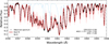 |
Fig. 1 Portion of the spectrum of star CES 1222+1136, showing the NH band at 3360 Å. The solid curves show the best fit with A(N) = 5.48 (thicker red line), and the red shaded areas display A(N) ± 0.30 dex. The dashed blue line represents the synthesis if N is fully removed. The atmospheric parameters Teff (K), log ɡ, [Fe/H], and υturb (km s−1) are shown in the lower right corner. |
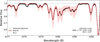 |
Fig. 2 Portion of the spectrum of star CES 1222+1136, showing the G band on the region 4277–4282 Å. The solid curves show the best fit with A(C) = 5.67 (thicker red line), and the red shaded areas display A(C) ± 0.30 dex. The dotted blue line represents the synthesis if C is fully removed. The atmospheric parameters Teff (K), log ɡ, [Fe/H], and υturb (km s−1) are shown in the lower right corner. |
5 Abundance results
The nine stars in our sample for which the Li line is measurable show very similar lithium abundances, with an average A(Li) = 1.04 ± 0.1 dex and low dispersion of σ = 0.06 dex. Our results for lithium at low metallicity are in good agreement with the measurements of Mucciarelli et al. (2022), where an average A(Li) = 1.06 ± 0.01 dex was found for 47 carbon-normal stars on the lower red giant branch (LRGB) in the metallicity range of −3.80 ≤ [Fe/H] ≤ −1.3 dex. It should also be highlighted that seven out of the nine stars for which we derived lithium abundances were also analyzed by Mucciarelli et al. (2022). Their results are in agreement with those found in this study within the errors.
The upper panel of Fig. 3 shows that A(Li) increases with increasing metallicity and the slope for the plot is equal to 0.14. If the star CES 1436–2906, with [Fe/H] = −2.15 dex, is excluded, the mean average for A(Li) does not change significantly while the slope increases to 0.31. The presence of this linear trend for lithium is possibly attributed to the small subsample of stars with Li features in our sample and could be erased by increasing the sample size. Moreover, the changes in the abundance of lithium in the considered metallicity domain do fit inside the error bar indicated in the lower right corner of the figure; therefore, the small linear change with metallicity is also compatible with a constant Li abundance. Adopting the 3D NLTE corrections, we obtained Li abundances slightly higher in comparison with the non-corrected abundances (lower panel in Fig. 3). In fact, the largest correction applied is 0.04 dex in A(Li), and the linear fit that correlates the uncorrected Li abundances with the corrected ones has a slope of ~ 0.91. Therefore, this difference (3D, NLTE correction) does not change the slope for A(Li) versus [Fe/H] and is not significant for our results.
Continuing with the CNO elements, the left panel in Fig. 4 shows the derived abundances for carbon compared to Fe I. The temperature range of the stars in our sample allowed us deriving carbon abundances using the molecular G-band for 42 out of the 52 stars. For the ten remaining stars, carbon measurements are not possible because their spectra do not cover the region between 4277 Å and 4330 Å and the atomic C III line at 5376.19 Å is too weak. The mean value of the ratio [C/Fe] is +0.063 dex with a scatter of σ = 0.366 dex. Our carbon abundances span from ~−0.58 to ~+0.58 dex and therefore there are no CEMP stars5 in the sample. This is, however, justified by the fact that we avoided selecting stars with strong carbon molecular features. The large scatter observed with respect to Fe is comparable to the one found when plotting [C/Mg] versus [Mg/H] (Fig. 5, upper panel).
The middle panel in Fig. 4 shows the relation between nitrogen and Fe I. The mean value <[N/Fe]> is 0.21 dex and the dispersion is 0.658 dex. This value is even greater than that found for C. The same occurs for the ratio [N/Mg] (Fig. 5, lower panel) where the dispersion of 0.630 dex is almost the same as for [N/Fe]. The large scatter found for [C/Fe] and [N/Fe] versus [Fe/H] may indicate that subsequent mixing episodes have altered the initial composition of the atmosphere in some stars.
For the star CES 1245–2425, also known as HE 1243–2408, we found an abundance of A(C) = 5.85 dex. This result is similar to the abundance derived in Shejeelammal & Goswami (2024) for the same star, where they found A(C) = 5.95 dex from spectral synthesis in the CH G-band at 4315Å and before applying evolutionary corrections in order to take into account the extra-mixing. With regards to nitrogen, however, our results show a large discrepancy, which might be due to the different nitrogen lines considered. We obtained an abundance of A(N) = 4.35 dex using the NH band, whereas Shejeelammal & Goswami (2024) obtained an upper limit of A(N)<8.33 by using the 12CN line at 4215Å.
As noted in Section 4.4, the two neutral oxygen lines used in this work are not affected by NLTE effects, in contrast with the predictions that ionized species are less affected by NLTE than the neutral ones (Amarsi et al. 2016b). Therefore, we plotted oxygen compared to Fe II (right panel of Fig. 4). We find that the ratio [O/Fe] declines linearly toward solar metallicities (Fig. 4), with [O/Fe] = 1.01 dex at [Fe/H] = −3.05 dex decreasing to [O/Fe] = 0.63 dex at [Fe/H] = −1.87 dex. The estimated slope is about −0.25. The mean value we found for oxygen is [O/Fe] ~ 0.77 dex and the dispersion of 0.10 dex is the lowest among those calculated for CNO. The average value obtained for oxygen abundances is close to that in Cayrel et al. (2004) for metal-poor halo stars, where they also used the forbidden oxygen line at 6300 Å.
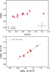 |
Fig. 3 Lithium abundances obtained with our 1D LTE analysis (red symbols) and corrected for 3D NLTE effects (violet open symbols) as a function of [Fe/H] for the stars in our sample (top). A representative error bar is plotted in the lower-right corner of the figure. In the lower panel, we compare both 1D LTE and 3D NLTE lithium abundances. The stars CES 1543+0201 and CES 2231–3238 overlap around log NLi = 1.04 and log NLi 3D NLTE = 1.07. |
6 Discussion
The stars may preserve information on the composition of the gas from which they formed if they have not evolved considerably. Metal-poor stars are of particular interest as these objects are likely a product of the earliest generation of stars formed in the Universe and can thus provide us with archaeological information about the evolution of the early Galaxy. However, the dredge-up events can alter their initial composition bringing material from deep layers to the surface. When the star ascend to RGB, the first dredge-up (FDU) occurs and the abundance of the light elements on the star’s surface is predicted to change (Iben 1964; Iben & Renzini 1984). Although this event is expected to be less efficient at low-metallicities (Charbonnel 1994), a second mixing episode takes place when the star becomes brighter than the RGB bump. This extra-mixing is responsible for destroying the remaining Li, as well as depleting 12C while increasing 14N, resulting in anomalous abundance patterns for these elements (Gratton et al. 2000). Therefore, it is important to know if the stars we are analyzing have gone through extra-mixing.
The location of our program stars along the HR diagram indicates that almost all of them are in the RGB phase (Fig. 6). The exception is the chemically peculiar star CES 2250-4057, which is likely a horizontal branch (HB) star6. In Paper I, we showed that the ratios [Y II/Sr II] and [Zr II/Sr II] for this star have the same pattern as other HB stars studied by Roederer et al. (2014). Interestingly, although these results suggest that the star CES 2250–4057 is a HB star, we found that it shows no sign of extra-mixing. We have used evolutionary tracks from BaSTI and MIST with [Fe/H] = −2.50 dex. Both tracks agree with the phase of the sample stars within the scatter and comparison with evolutionary tracks accounting for rotation does not show any detectable difference compared to those with Vrot = 0 for our low-mass stars. We adopted the models for 0.8-M⊙ stars, however, using the tracks with masses ranging from ~0.6 to ~ 1.2 M⊙ does not significantly change the evolutionary stage of our RGB stars. The color code with regard to carbon-nitrogen ratios shows that the spectroscopically observed [C/N] decreases from the base to the tip of the RGB. It is also important to state that this ratio changes due to both the increasing [N/H] and the decreasing [C/H]. Such abundance changes on the stellar surface have been observed in metal-poor stars and indicate deep mixing taking place in the stars during the RGB phase (Gratton et al. 2000; Martell et al. 2008).
6.1 Carbon and nitrogen
During the CNO cycle, N is produced at the expense of C. The FDU will enrich the surface of the star and turn the atmosphere of the star rich in 14N and poor in 12C, relative to its initial composition. As a result, carbon and nitrogen can be used as mixing indicators (e.g., Gratton et al. 2000; Korn et al. 2006). Abundance changes in N at the expense of O are not expected because the ON-cycle occurs in a region deeper than the CN-cycle and requires higher temperatures than the temperatures involved in our low-mass stars.
rom our results for carbon and nitrogen shown in Table A.1, it is evident that some of the stars exhibit an enrichment of nitrogen and a depletion of carbon. In fact, the mean average abundance found for nitrogen is relatively higher than that found for carbon. This behavior is seen more clearly when plotting [N/Fe] against [C/Fe] (Fig. 7). In spite of this, there is no fully clear separation between the stars that could indicate internal mixing. Although we have considered all the stars in the sample, comprising different metallicities, the plots for given bins of metallicities in the range of ~0.5 dex (Figs. D.2 and D.3) still do not show a clear distinction. By adopting the limits defined by Spite et al. (2005), the distinction between mixed and unmixed stars, however, becomes more clear, especially if we are taking into account the error bars estimated for the stars (σ[C/Fe] = ±0.18 dex and σ[N/Fe] = ±0.22 dex). We have found that only two out of the 35 stars for which we obtained both carbon and nitrogen abundances could not be classified according to the limits from Spite et al. (2005). These stars are CES 0221–2130 with [C/Fe] = −0.35 dex and [N/Fe] = +0.17 dex and CES 0424–1501, with [C/Fe] = −1.94 dex and [N/Fe] = −0.11 dex (blue filled circles in the figures) and are the most metal-rich stars in the sample with carbon and nitrogen measurements. Another four stars are classified as unmixed within the abundance uncertainties (encircled stars). Additionally, we have five more stars with no carbon measurements, which we classified as unmixed due to the presence of Li in their atmospheres.
When plotting [C/Fe] against the effective temperature and log ɡ (upper panels in Fig. 8), it is noticeable that the sample splits in two distinct groups following our classification. The diagram is color-coded according to the mixing, which shows that there is a plateau around [C/Fe] ~0.4dex for the unmixed stars; however, there is an exception for the stars CES 0527–2052, CES 1222−1136, CES 1413–7609, and CES 2254–4209, which are placed along with the mixed stars. These four outliers are the unmixed stars that are the closest to the “mixed region” in Fig. 7 (circled symbols) and two of them could also be classified as mixed stars considering the estimated uncertainties for both carbon and nitrogen. Moreover, they are located after the RGB bump (yellow dashed lines in Fig. 8), where extra-mixing begins due to thermohaline instability (Charbonnel & Zahn 2007). Hence, these stars are likely to have completed the FDU and have begun to experience extra-mixing, even though carbon depletion and nitrogen enrichment are moderate. Regarding the mixed stars, although they are clearly separated from the flat trend displayed by the unmixed stars, they have a more scattered distribution with no tendency to lower [C/Fe] ratios toward lower temperatures – as would be expected from deep mixing.
In contrast, the plots for [N/Fe] versus Teff and log ɡ trends (middle panels in Fig. 8) do not follow the above-mentioned behavior. Instead, they display a single linear trend for both classes of stars regardless of the outliers. As the trends for N are steeper than the ones observed for carbon, this could indicate that maybe the ON-cycle has taken place and converted some O into N. However, the lower panels show that oxygen remains constant with the temperature and log ɡ and the fewer unmixed stars observed in the plot do not allow statistically solid inferences.
By plotting C, N, and O in terms of [X/H] (see Fig. D.1) we obtained a wider spread in the figure, yet the trends with temperature and surface gravity remain. One possible scenario to explain this is that these stars have been formed in clouds with different pre-existing carbon and nitrogen reservoirs and therefore not all nitrogen observed on their surfaces is a product of deep mixing. Another possibility is that this could be evidence of primary N production.
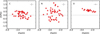 |
Fig. 4 Elemental abundances for C, N, and O plotted as a function of [Fe/H] for the stars in our sample. A representative error bar is plotted in the upper right corner of each panel. |
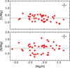 |
Fig. 5 [C/Mg] and [N/Mg] as a function of [Mg/H] for the stars in our sample. A representative error bar is plotted in the upper-right corner of each panel. |
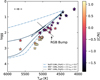 |
Fig. 6 CERES stars in the Teff − log ɡ diagram. The BaSTI evolutionary track (blue dash-dotted line) has an α-enhanced chemical mixture and does not include rotation. Two MIST evolutionary tracks are also included for non-rotating (blue continuous line) and with rotation vcrit = 0.4 (gray dotted line). All the tracks are for M = 0.8 M⊙ and [Fe/H] = −2.50 dex. The RGB Bump for the adopted tracks is at Teff ~ 4880 K and log ɡ ~1.95 dex. The color index on the right side of the figure indicates the [C/N] abundance ratio. The dispersion in Teff and log ɡ measurements is represented by the error bar in the upper left corner of the figure. |
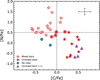 |
Fig. 7 [N/Fe] versus [C/Fe] for our sample. The mixed and unmixed stars are classified based on Spite et al. (2005) and considering the estimated uncertainties for each element. The open red star markers represent the mixed stars, while the filled red star markers represent the unmixed stars; the violet triangles are the unmixed stars for which we also found Li abundances; and the blue hexagons are the stars CES 0221–2130 and CES 0424–1501 outside the adopted limits for mixed and unmixed stars. The encircled red stars marker are unmixed stars classified within the abundance uncertainties and are located after the RGB Bump in the HR diagram. A representative error bar is plotted in the upper-right corner of the figure. |
6.2 Carbon and nitrogen versus oxygen
Different mechanisms taking place in stars of different mass ranges are responsible for producing the CNO elements. As a consequence, the [C/O] and [N/O] ratios measured in low-metallicity stars in the Galaxy exhibit a remarkable deviation from 0 (see e.g., Cayrel et al. 2004; Spite et al. 2005; Nissen et al. 2014; Amarsi et al. 2019a,b). The ratios [C/O] and [N/O] can be of particular interest for studying the chemical evolution of galaxies (see Sect. 6.5).
Figure 9 shows [C/O] ratios as a function of [O/H] for both mixed and unmixed stars in our sample. Oxygen is mainly produced in massive stars on short timescale (Kobayashi et al. 2006; Cescutti et al. 2009), so that the plot for [C/O] against [O/H] depends mainly on the yields and timescale of carbon production and can thus offer clues on carbon evolution. It has been shown that at lower metallicities, the ratio [C/O] increases with decreasing [O/H] (Akerman et al. 2004; Fabbian et al. 2009). However, the 3D non-LTE analysis (Amarsi et al. 2019b) seems to contradict these results. This trend might be connected to the carbon-rich yields from the massive Population III stars (Ishigaki et al. 2014); alternatively, these metal-poor stars could be fast rotators (Meynet et al. 2006; Chiappini et al. 2006). Although these observations disagree with the predictions of some chemical evolution models (Chiappini et al. 2003; Gavilán et al. 2005), slow-rotating stellar models at Z = 10−5 have shown that [C/O] ratios might increase with increasing [O/H] Ekström et al. (2008). It would be interesting also to investigate [C/O] ratios relatively to [O/H] for the unmixed stars; unfortunately, we have managed to measure oxygen only for two of the stars that fall into the unmixed stars group and any further interpretation is not possible. However, the [C/O] ratios for these two stars are in good agreement with results from literature for halo stars.
The behavior of the ratio [N/O] relative to the metallicity is associated to the nature of nitrogen. Stellar studies at low metallicities have found that the abundance of primary nitrogen remains constant with respect to [O/H] (Israelian et al. 2004; Spite et al. 2005) but here we find quite some scatter around the flat trend. However, if the nitrogen production were dominated by secondary mechanisms, one should expect nitrogen abundances proportional to [O/H] ratios (Edmunds & Pagel 1978; Papadopoulos 2010; Roy et al. 2021). In Fig. 10, we compare the [N/O] and [O/H] ratios. Here, again, any statistical analysis is limited by the small number of [N/O] ratios we obtained for the stars in our sample. Additionally taking into account the stars for which we have Li abundances despite the absence of carbon abundances, we have [N/O] ratios for four unmixed stars. In comparison with results from literature, our stars also show a good agreement, although the two unmixed stars classified from Li abundances have lower [N/O] ratios.
6.3 Lithium
Lithium was primordially synthesized in the Big Bang nucleosynthesis and is easily destroyed at temperatures higher than 2.5 × 10⁶ K. This means that Li can be preserved only in the atmosphere of the stellar surface in evolved stars, not in their interiors. After the main sequence, when the star ascends to the RGB and goes through the FDU, mixing processes are responsible for destroying the Li present on the surface of the star, reducing the observed Li abundance of the star. Therefore, it is also possible to probe deep mixing from Li abundances. Measurements of Li abundances were possible for only nine stars in our sample (Fig. 3). All these stars show A(Li) ≤ 0.94 and a mean of 1.02 with low dispersion. We were able to prove mixing for four out of these nine stars. According to the adopted limits, these four stars have Li abundances compatible with unmixed stars, namely, [N/Fe] < 0.5 dex and [C/N] > −0.6 dex. For the other five stars, no measurements of carbon or nitrogen were possible. In contrast, we did not detect lithium in any of the mixed stars ([N/Fe] > 0.5 dex and [C/N] < −0.6 dex).
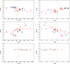 |
Fig. 8 [C/Fe] as a function of the effective temperature (on the left) and the surface gravity (on the right) for all the stars in our sample (top). A clear separation can be seen between the mixed and unmixed stars, except for the four encircled stars. [N/Fe] with respect to Teff and log ɡ are shown in the middle panels. The lower panel shows [O/Fe] as a function of Teff and log g. The yellow dashed line indicates the Teff and log ɡ at the RGB bump. The blue symbols represent the stars for which we could not classify from C and N, therefore, the blue symbols in the [C/Fe] plots not necessarily are the same stars seen in the plot [N/Fe], Symbols are the same as in Fig. 7. |
6.4 Rotation
Rotation has been proven to play a key role in reproducing the evolution of massive stars at very low metallicities (e.g., Meynet et al. 2006; Chiappini et al. 2006). The high rotation rates are responsible for internal mixing, leading to a large production of 14N and 13C (Meynet et al. 2006). As a consequence, higher carbon-to-nitrogen ratios should be expected in non-rotating stars with respect to their counterparts that have gone through rotational mixing. In this sense, if the clouds where the stars in our sample have formed were made up of material enriched by previous rotating models, our unmixed stars (i.e., stars whose surface abundances directly reflect the abundances of the material from which they were formed) would be expected to show lower C/N ratios than stars made from material enriched by slowly or non-rotating models. This behavior is well reproduced by the stars in our sample as shown in the upper panel of Fig. 11. The plot appears to follow a trend to lower [C/N] ratios with decreasing Teff. The stars that fall into the mixed stars group populate the region further down below [C/N] <−0.6 dex, while the ones in the unmixed stars group have [C/N] ratios above this value. These results are in good agreement with the predictions of Lagarde et al. (2017, 2019) using the Besançon Galaxy model, accounting for thermohaline instability effects on the theoretical [C/N] ratios along the RGB. Here, we note two things, namely, that we are neglecting possible differences in initial stellar enrichment (e.g., from massive stars with or without rotation) and there is a region between ~4800 – 5100 K where the mixed and unmixed groups overlap.
Berg et al. (2016, 2019) have found that the C/N ratio shows a flat trend at log(C/N) ~ 0.90 (whatever the metallicity) but with a significant scatter (σ ~ 0.5). This plateau may indicate that carbon and nitrogen are produced by the same nucleosynthetic mechanisms. In plotting log(C/N) versus [Fe/H] for our unmixed stars (lower panel of Fig. 11), we also find that the C/N ratio is almost constant with the metallicity (log(C/N) ~ 0.94) and a scatter of 0.54, close to the observations by Berg et al.
Beyond the contribution to the light element abundances, the mixing induced by rotation also leads to a great enhancement of 22Ne (Meynet et al. 2006). This may, in turn, contribute with neutrons to the weak s-process through the reaction 22Ne(α, n)25Mg, causing an overproduction of light s-process elements as Sr, Y, and Zr (Chiappini et al. 2011; Frischknecht et al. 2012). However, this does not seem to be the case of our stars (Paper I). Moreover, we see no clear trend in Sr, Y, or Zr as a function of [C/H], [N/H], or [C/N] regardless of the mixing or evolutionary stage (see Fig. 12)7.
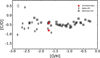 |
Fig. 9 [C/O] ratios versus [O/H] for the stars in our sample. Gray symbols represent [C/O] ratios derived in Spite et al. (2005) (diamond symbols) and Akerman et al. (2004) (square symbols). |
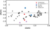 |
Fig. 10 [N/O] ratios versus [O/H] for the stars in our sample. Gray symbols represent [N/O] ratios derived in Spite et al. (2005) (diamond symbols) and Akerman et al. (2004) (square symbols). |
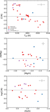 |
Fig. 11 [C/N] ratios as a function of Teff (top). The dashed line at [C/N] = −0.6 dex separates the mixed and unmixed stars. Middle panel: [N/Mg] ratios as a function of [Mg/H]. The horizontal dashed line at [N/Mg] = ~0.43 dex indicates the mean value for the ratio [N/Mg]. Lower panel: log(C/N) as a function of [Fe/H]. Symbols are the same as in Fig. 7. A representative error bar is plotted in the upper-right corner of the panels. |
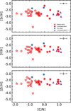 |
Fig. 12 Light s-process elements Sr, Y, and Zr as a function of [C/N] for the stars in our sample. A representative error bar is plotted in the upper-left corner of the figure. Symbols are indicated in the upper panel of this figure and are the same as in Fig. 7. |
6.5 Comparison with chemical evolution model results
Hereafter, we present our comparison of the abundance data given in the previous sections with the predictions of a GCE model. The model assumes that the thick- and thin-disc components of the Milky Way form sequentially, out of two main episodes of gas accretion (two-infall model, Chiappini et al. 1997, 2001; Romano et al. 2010; Spitoni et al. 2019). We adopted the latest version of the model, which includes constraints on stellar ages from asteroseismology (Spitoni et al. 2019, 2021, and references therein). In particular, the delay time for the second infall is fixed to a much higher value (3.25 Gyr) than assumed in the original formulation (1 Gyr). The infalling gas is accreted smoothly, following an exponentially decaying law. In the solar vicinity, the e-folding time scales are 1 and 7 Gyr for the thick-and thin-disc components, respectively. The star formation rate is expressed as a Kennicutt (1998) law,
 (1)
(1)
where σgas(t) is the surface gas density at any time and k = 1.5. The adopted galaxy-wide stellar initial mass function (gwIMF) is that of Kroupa et al. (1993).
The most important ingredients of any GCE model are the stellar yields, though. For the present study, mostly concerned with the chemical composition of metal-poor stars, we fixed the yields of low- and intermediate-mass stars (taken from the FRUITY web-based database, Cristallo et al. 2009, 2011, 2015) and explore different nucleosynthesis prescriptions for massive stars.
First, we considered the recommended yield set (set R) of Limongi & Chieffi (2018). These authors computed the presupernova evolution and explosive nucleosynthesis of massive star models covering the initial mass range 13–120 M⊙ for different initial chemical compositions (corresponding to [Fe/H] = −3, −2, −1, and 0) and rotational velocities of the stars (υrot = 0, 150, and 300 km s−1). In set R, the mixing and fallback scheme (Umeda & Nomoto 2002) was adopted for all stars in the initial mass range 13–25 M⊙. The inner border of the mixed zone was set at the layer where [Ni/Fe] = 0.2 dex, while the outer border was fixed at the base of the O shell. The mass cut is then set by the assumption that each star ejects 0.07 M⊙ of Ni. Stars more massive than 25 M⊙ collapse to black holes; thus, their yields consist of the sole wind contribution. The impact of massive star rotation on the evolution of CNO isotopes predicted by adopting Limongi & Chieffi (2018) yields is extensively discussed in Romano et al. (2019, 2020). The light pink, pink, and violet lines in Fig. 13 show the predictions of the GCE model implementing Limongi & Chieffi (2018) yields for massive stars with υrot = 0, 150, and 300 km s−1, respectively. It is seen that the model that does not include fast rotators predicts abundance trends completely offset from the data, due to the well documented underproduction of N when rotation is not included in the massive stars models (Chiappini et al. 2006; Romano et al. 2010, 2019; Prantzos et al. 2018; Kobayashi et al. 2020).
The yield set R of Limongi & Chieffi (2018) covers homogeneously an extended range of initial masses, metallicities and rotational velocities, and allows studying a number of nuclear species. Other studies in the literature investigate the modifications in stellar nucleosynthesis triggered by rotation, but are limited to the pre-SN stages and/or to a few chemical elements (e.g., Meynet & Maeder 2002; Hirschi et al. 2005; Hirschi 2007; Ekström et al. 2008). Nonetheless, these yields have been included in GCE models, providing interesting clues on the origin of 14N and 13C in the solar vicinity (Chiappini et al. 2006; Romano et al. 2010) and across the whole Galactic disc (Romano et al. 2017). In this work, we tested the latest generation of stellar models by the Geneva group (using the Geneva stellar evolution code or GENEC8), by implementing in the adopted GCE code yields for massive stars, in the mass range of 9 M⊙ ≤slantMini ⩽ 120 M⊙, which are either rotating9 (dark green and dark-blue lines in Fig. 13) or non-rotating models (light-green and light blue lines in Fig. 13). We included stellar grids from extremely metal-poor up to super-solar metallicity (more details in Ekström et al. 2012; Georgy et al. 2013; Groh et al. 2019; Sibony et al. 2024).
To calculate the stellar yields, either during the lifetime or at the end of it, we need to define the mass cut, which is the limit below which everything will be locked in the stellar remnant, while the rest will be ejected to the ISM. We investigate the effects of changing the mass cut location. Thus, we followed two ways of defining the mass cut, either from Patton & Sukhbold (2020), shown as dashed greenish curves in Fig. 13, or from Maeder (1992), shown as dashed blueish curves in Fig. 13. For both cases, it is necessary to calculate the CO core mass (Mco) of the models, which is defined where the mass fraction of helium drops below 0.0110. Having the remnant masses, we obtain the stellar yields by integrating above the mass cut and by subtracting the initial abundance of the isotopes. It is found, again, that stellar rotation boosts the production of N at low metallicities, which improves the agreement between theoretical predictions and observational data. Moreover, it is found that the adopted mass cut location strongly influences primary N production from rotating massive star models otherwise sharing the same initial rotational velocity.
In Fig. 14, we present the stellar yields in M⊙ as calculated in Tsiatsiou et al. (in prep.) and used for the GCE models in Fig. 13. We compare the stellar yields from GENEC models (Georgy et al. 2013) with those from Limongi & Chieffi (2018) for the non-rotating models. The two different prescriptions for calculating the remnant masses in the GENEC models are represented by blue curves (Maeder 1992) and green curves (Patton & Sukhbold 2020). By comparing non-rotating models, we can eliminate differences due to the physics of rotation. We note here that in Limongi & Chieffi (2018), for models with initial masses above 25 M⊙, only the stellar winds are taken into account since these stars are assumed to form black holes that swallow the entire mass of the star at core collapse. The same applies to the GENEC models from Maeder (1992). However, in the GENEC models, when the remnant mass is computed according to Patton & Sukhbold (2020), models with initial masses above 20 M⊙ are assumed to become black holes; however, not all of the final mass of the star is swallowed by the black hole. Significant portions of the star’s mass can be lost through the supernova explosion prior to the black hole formation.
By examining Fig. 13, we observe that the differences in the stellar yields of the CNO elements between the GENEC models and the Limongi & Chieffi (2018) tracks can be attributed to differences in overshooting parameters, mass loss prescriptions, and the final evolutionary stages. For example, the GENEC models are not computed until the pre-supernova stage. Despite these differences, we see that the yields of 12C are similar. However, there is a significant exception for the 20 M⊙ model, which shows a very small 12C yield when the remnant mass is determined using the prescription by Patton & Sukhbold (2020). Similar values were also obtained for the yields of 14N for stars with initial masses below about 60 M⊙. The differences in the mass seen above likely result from variations in the stellar wind prescriptions, especially the metallicity dependence of the stellar winds. The yields of 16O are very similar, with the same remark regarding the differences shown by the 20 M⊙ model computed using the prescription by Patton & Sukhbold (2020) for the determination of the remnant mass.
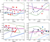 |
Fig. 13 [C/N] ratios as a function of [C/H] (top left panel), [O/H] (top right panel), and [N/H] (bottom left panel) for the unmixed stars in our sample. The bottom right panel shows [N/O] ratios as a function of [O/H] for the unmixed stars in our sample. Abundance ratios from Spite et al. (2005) (gray diamond symbols) and Israelian et al. (2004) (gray square symbols) for low-metallicity stars are also shown in the figures. The continuous lines are the predictions of GCE models using Limongi & Chieffi (2018) yields for massive stars with rotational velocities of vrot = 0 (LCOOO), 150 km s−1 (LC150), and 300 km s−1 (LC300); whereas the dashed lines correspond to GCE model predictions obtained using yields from GENEC stellar models with Patton & Sukhbold (2020) and Maeder (1992) mass cut prescriptions for non-rotating (PS and MAEDER, respectively) and rotating stars (PSrot and MAEDERRot, respectively). The models are color-coded as indicated in the top of the figure. A representative error bar is plotted in the lower right corner of each panel. |
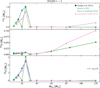 |
Fig. 14 Stellar yields in M⊙ for CNO elements for non-rotating models with [Fe/H] = −1, from GENEC models (diamonds, Georgy et al. 2013) and Limongi & Chieffi (2018) (triangles, pink curves). The models have an initial mass range of 9 M⊙ ≤slant Mini ⩽ 120 M⊙. The blue curves of GENEC models correspond to the Maeder (1992) prescription of calculating the remnant mass, and the green curves to the Patton & Sukhbold (2020). |
7 Conclusions
In this work, we have performed a detailed chemical analysis of the surface abundances of carbon, nitrogen, oxygen, and lithium in a sample of 52 halo stars with metallicities in the range −3.49 ≤[Fe/H] ≤ −1.79 dex. Our individual abundances presented here were computed under the ID LTE assumption. The 3D NLTE corrections for lithium calculated by Wang et al. (2021) did not significantly impact our results.
The star CES 2250–4057 is the only star in our sample lying in the region associated with the horizontal branch. It has been shown in Paper I that this is a striking star with an overabundance of Sr with respect to Y and Zr, while all abundances are low on a relative scale. In addition, we found that this star has mild carbon and nitrogen enrichment with [C/Fe] = 0.18 dex and [N/Fe] = 0.17 dex and, thus, does not show traces of deep mixing according to our classification.
Our RGB stars can be split in three different groups. The group of mixed stars have an overabundance of nitrogen and carbon depletion showing clear signs that the CN-cycle processed material was brought to the surface of these stars. Additionally, we found no signature that could indicate that the ON-cycle took place. According to the temperature and surface gravities of these stars, these stars are on the upper RGB, after the RGB Bump, showing deep mixing and confirming the results on extra-mixing (Gratton et al. 2000).
The stars classified as unmixed (see Spite et al. 2005) show no signature of CNO processed material at their surfaces and exhibit [C/N] ratios lower than −0.50 dex. The presence of lithium on the surface of nine of the unmixed stars was also used to probe the mixing (and the abundance values confirm that they are unmixed). Almost all these stars lie on the lower RGB with temperatures and surface log ɡ above ~4880 K and ~ 1.95 dex, respectively. However, for four unmixed stars, we found that they approach the upper RGB and their [N/Fe] ratios are close to our adopted limits. This may indicate that the signature of mixing due to the CNO burning layers is not yet significant.
The last group consists of stars that we did not manage to classify given the lack of carbon or nitrogen and also lithium. These stars show no particular behavior when plotted along with the other stars of the sample and (according to their position on the HR diagram) it is likely that some of them have experienced deep mixing. When considering heavy elements Sr, Y, and Zr, neither of the three mixing groups show specific trends as a function of [C/N]. This may indicate that these heavy elements do not suffer detectable changes in the stellar surface for stars with our sample stellar parameters. It is important to know that the nucleosynthetic imprints of heavy elements remain unaltered by stellar evolution processes and the abundances can directly be used to trace the underlying neutron capture processes.
We computed homogeneous GCE models to trace the evolution of carbon, nitrogen, and oxygen in our Galaxy. We confirm that models taking stellar rotation into account fit the average runs of abundance ratios for unmixed stars better than models that do not consider the effects of rotation. We also find that the location of the mass cut influences the exact amount of primary N ejected by low-metallicity stars, at a fixed initial rotational velocity.
Acknowledgements
We thank the anonymous referee for the useful comments and suggestions that helped to improve this work. RFM, AAP, LL, and CJH acknowledge the support by the State of Hesse within the Research Cluster ELEMENTS (Project ID 500/10.006). CJH also acknowledges the European Union’s Horizon 2020 research and innovation program under grant agreement No 101008324 (ChETEC-INFRA). ST and GM have received funding from the European Research Council (ERC) under the European Union’s Horizon 2020 research and innovation program (grant agreement No 833925, project STAREX). DR acknowledges the support by the Italian National Institute for Astrophysics (INAF) through Finanziamento della Ricerca Fondamentale, Theory Grant Fu. Ob. 1.05.12.06.08 (Project “An in-depth theoretical study of CNO element evolution in galaxies”).
Appendix A Abundances
Chemical abundances derived in this work.
Appendix B Atmospheric parameters
Stellar parameters from Lombardo et al. (2022) for the stars in our sample.
Appendix C Slopes
Slopes for the s-elements Sr, Y, and Zr with respect to the [C/N] ratios.
Appendix D Supplementary figures
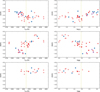 |
Fig. D.1 [C/H] as a function of the effective temperature (on the left) and the surface gravity (on the right) for all the stars in our sample (top). A clear separation can be seen between the mixed and unmixed stars, with the exception of the four encircled stars. [N/H] with respect to Teff and log ɡ are shown in the middle panels. The lower panel shows [O/H] as a function of Teff and log ɡ. The yellow dashed line indicates the Teff and log ɡ at the RGB bump. Symbols are the same as in Fig.7. Using H instead of Fe makes our unmixed stars are spreader, however it does not vanish the separation between mixed and unmixed. |
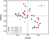 |
Fig. D.2 [N/Fe] versus [C/Fe] for our sample stars divided in metallicity bins (see the legend in the bottom left corner of the figure). We could not find any trends that could indicate a dependence of stellar mixing on metallicity. However, the stars we could not classify following the adopted limits are the most metal-rich ones of our sample. A representative error bar is plotted in the upper right corner of the figure. |
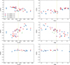 |
Fig. D.3 [C/Fe] as a function of the effective temperature (on the left) and the surface gravity (on the right) for all the stars in our sample (top). [N/Fe] with respect to Teff and log ɡ are shown in the middle panels. The lower panel shows [O/H] as a function of Teff and log ɡ. The yellow dashed line indicates the Teff and log ɡ at the RGB bump. As in Fig. D.2, by plotting for different bins of metallicity, we could not find trends for the mixing and unmixed stars. |
References
- Akerman, C. J., Carigi, L., Nissen, P. E., Pettini, M., & Asplund, M. 2004, A&A, 414, 931 [NASA ADS] [CrossRef] [EDP Sciences] [Google Scholar]
- Amarsi, A. M., Asplund, M., Collet, R., & Leenaarts, J. 2016a, MNRAS, 455, 3735 [NASA ADS] [CrossRef] [Google Scholar]
- Amarsi, A. M., Lind, K., Asplund, M., Barklem, P. S., & Collet, R. 2016b, MNRAS, 463, 1518 [NASA ADS] [CrossRef] [Google Scholar]
- Amarsi, A. M., Nissen, P. E., Asplund, M., Lind, K., & Barklem, P. S. 2019a, A&A, 622, L4 [NASA ADS] [CrossRef] [EDP Sciences] [Google Scholar]
- Amarsi, A. M., Nissen, P. E., & Skúladóttir, Á. 2019b, A&A, 630, A104 [NASA ADS] [CrossRef] [EDP Sciences] [Google Scholar]
- Arcones, A., & Thielemann, F.-K. 2023, A&A Rev., 31, 1 [NASA ADS] [CrossRef] [Google Scholar]
- Bailer-Jones, C. A. L., Rybizki, J., Fouesneau, M., Demleitner, M., & Andrae, R. 2021, AJ, 161, 147 [Google Scholar]
- Berg, D. A., Skillman, E. D., Henry, R. B. C., Erb, D. K., & Carigi, L. 2016, ApJ, 827, 126 [NASA ADS] [CrossRef] [Google Scholar]
- Berg, D. A., Erb, D. K., Henry, R. B. C., Skillman, E. D., & McQuinn, K. B. W. 2019, ApJ, 874, 93 [NASA ADS] [CrossRef] [Google Scholar]
- Burbidge, E. M., Burbidge, G. R., Fowler, W. A., & Hoyle, F. 1957, Rev. Mod. Phys., 29, 547 [NASA ADS] [CrossRef] [Google Scholar]
- Caffau, E., Faraggiana, R., Ludwig, H. G., Bonifacio, P., & Steffen, M. 2011, Astron. Nachr., 332, 128 [NASA ADS] [CrossRef] [Google Scholar]
- Casagrande, L., & VandenBerg, D. A. 2018, MNRAS, 479, L102 [NASA ADS] [CrossRef] [Google Scholar]
- Cayrel, R., Depagne, E., Spite, M., et al. 2004, A&A, 416, 1117 [NASA ADS] [CrossRef] [EDP Sciences] [Google Scholar]
- Cescutti, G., Matteucci, F., McWilliam, A., & Chiappini, C. 2009, A&A, 505, 605 [NASA ADS] [CrossRef] [EDP Sciences] [Google Scholar]
- Charbonnel, C. 1994, A&A, 282, 811 [NASA ADS] [Google Scholar]
- Charbonnel, C., & Zahn, J. P. 2007, A&A, 467, L15 [NASA ADS] [CrossRef] [EDP Sciences] [Google Scholar]
- Chiappini, C., Matteucci, F., & Gratton, R. 1997, ApJ, 477, 765 [Google Scholar]
- Chiappini, C., Matteucci, F., & Romano, D. 2001, ApJ, 554, 1044 [NASA ADS] [CrossRef] [Google Scholar]
- Chiappini, C., Romano, D., & Matteucci, F. 2003, MNRAS, 339, 63 [NASA ADS] [CrossRef] [Google Scholar]
- Chiappini, C., Hirschi, R., Meynet, G., et al. 2006, A&A, 449, L27 [NASA ADS] [CrossRef] [EDP Sciences] [Google Scholar]
- Chiappini, C., Frischknecht, U., Meynet, G., et al. 2011, Nature, 472, 454 [Google Scholar]
- Collet, R., Asplund, M., & Trampedach, R. 2007, A&A, 469, 687 [NASA ADS] [CrossRef] [EDP Sciences] [Google Scholar]
- Cristallo, S., Straniero, O., Gallino, R., et al. 2009, ApJ, 696, 797 [NASA ADS] [CrossRef] [Google Scholar]
- Cristallo, S., Piersanti, L., Straniero, O., et al. 2011, ApJS, 197, 17 [NASA ADS] [CrossRef] [Google Scholar]
- Cristallo, S., Straniero, O., Piersanti, L., & Gobrecht, D. 2015, ApJS, 219, 40 [Google Scholar]
- Dekker, H., D’Odorico, S., Kaufer, A., Delabre, B., & Kotzlowski, H. 2000, SPIE Conf. Ser., 4008, 534 [Google Scholar]
- Edmunds, M. G., & Pagel, B. E. J. 1978, MNRAS, 185, 77P [NASA ADS] [CrossRef] [Google Scholar]
- Eggenberger, P., Meynet, G., Maeder, A., et al. 2008, Ap&SS, 316, 43 [Google Scholar]
- Ekström, S., Meynet, G., Chiappini, C., Hirschi, R., & Maeder, A. 2008, A&A, 489, 685 [NASA ADS] [CrossRef] [EDP Sciences] [Google Scholar]
- Ekström, S., Georgy, C., Eggenberger, P., et al. 2012, A&A, 537, A146 [Google Scholar]
- Fabbian, D., Nissen, P. E., Asplund, M., Pettini, M., & Akerman, C. 2009, A&A, 500, 1143 [NASA ADS] [CrossRef] [EDP Sciences] [Google Scholar]
- Farmer, R., Laplace, E., de Mink, S. E., & Justham, S. 2021, ApJ, 923, 214 [NASA ADS] [CrossRef] [Google Scholar]
- Frischknecht, U., Hirschi, R., & Thielemann, F. K. 2012, A&A, 538, L2 [NASA ADS] [CrossRef] [EDP Sciences] [Google Scholar]
- Gaia Collaboration (Prusti, T., et al.) 2016, A&A, 595, A1 [NASA ADS] [CrossRef] [EDP Sciences] [Google Scholar]
- Gaia Collaboration (Babusiaux, C., et al.) 2018, A&A, 616, A10 [NASA ADS] [CrossRef] [EDP Sciences] [Google Scholar]
- Gaia Collaboration (Brown, A. G. A., et al.) 2021, A&A, 649, A1 [NASA ADS] [CrossRef] [EDP Sciences] [Google Scholar]
- Gavilán, M., Buell, J. F., & Mollá, M. 2005, A&A, 432, 861 [NASA ADS] [CrossRef] [EDP Sciences] [Google Scholar]
- Georgy, C., Ekström, S., Eggenberger, P., et al. 2013, A&A, 558, A103 [NASA ADS] [CrossRef] [EDP Sciences] [Google Scholar]
- Gratton, R. G., Sneden, C., Carretta, E., & Bragaglia, A. 2000, A&A, 354, 169 [NASA ADS] [Google Scholar]
- Groh, J. H., Ekström, S., Georgy, C., et al. 2019, A&A, 627, A24 [NASA ADS] [CrossRef] [EDP Sciences] [Google Scholar]
- Hansen, C. J., Hansen, T. T., Koch, A., et al. 2019, A&A, 623, A128 [NASA ADS] [CrossRef] [EDP Sciences] [Google Scholar]
- Hirschi, R. 2007, A&A, 461, 571 [NASA ADS] [CrossRef] [EDP Sciences] [Google Scholar]
- Hirschi, R., Meynet, G., & Maeder, A. 2005, A&A, 433, 1013 [NASA ADS] [CrossRef] [EDP Sciences] [Google Scholar]
- Hoyle, F. 1954, ApJS, 1, 121 [NASA ADS] [CrossRef] [Google Scholar]
- Huber, K. P. & Herzberg, G. 1979, Constants of Diatomic Molecules (Boston, MA: Springer US), 8 [Google Scholar]
- Iben, I., & Renzini, A. 1984, Phys. Rep., 105, 329 [NASA ADS] [CrossRef] [Google Scholar]
- Iben, Icko, J. 1964, ApJ, 140, 1631 [NASA ADS] [CrossRef] [Google Scholar]
- Israelian, G., Ecuvillon, A., Rebolo, R., et al. 2004, A&A, 421, 649 [NASA ADS] [CrossRef] [EDP Sciences] [Google Scholar]
- Ishigaki, M. N., Aoki, W., Arimoto, N., & Okamoto, S. 2014, A&A, 562, A146 [NASA ADS] [CrossRef] [EDP Sciences] [Google Scholar]
- Karakas, A. I., & Lattanzio, J. C. 2014, PASA, 31, e030 [NASA ADS] [CrossRef] [Google Scholar]
- Kennicutt J., Robert C., 1998, ApJ, 498, 541 [NASA ADS] [CrossRef] [Google Scholar]
- Kobayashi, C., Karakas, A. I., & Lugaro, M. 2020, ApJ, 900, 179 [Google Scholar]
- Kobayashi, C., Umeda, H., Nomoto, K., Tominaga, N., & Ohkubo, T. 2006, ApJ, 653, 1145 [NASA ADS] [CrossRef] [Google Scholar]
- Koch-Hansen, A. J., Hansen, C. J., Lombardo, L., et al. 2021, A&A, 645, A64 [NASA ADS] [CrossRef] [EDP Sciences] [Google Scholar]
- Korn, A. J., Grundahl, F., Richard, O., et al. 2006, Nature, 442, 657 [Google Scholar]
- Korn, A. J., Grundahl, F., Richard, O., et al. 2007, ApJ, 671, 402 [NASA ADS] [CrossRef] [Google Scholar]
- Kroupa, P., Tout, C. A., & Gilmore, G. 1993, MNRAS, 262, 545 [NASA ADS] [CrossRef] [Google Scholar]
- Kurucz, R. L. 2005, Mem. Soc. Astron. Ital. Suppl., 8, 14 [Google Scholar]
- Lagarde, N., Robin, A. C., Reylé, C., & Nasello, G. 2017, A&A, 601, A27 [NASA ADS] [CrossRef] [EDP Sciences] [Google Scholar]
- Lagarde, N., Reylé, C., Robin, A. C., et al. 2019, A&A, 621, A24 [NASA ADS] [CrossRef] [EDP Sciences] [Google Scholar]
- Limongi, M., & Chieffi, A. 2018, ApJS, 237, 13 [NASA ADS] [CrossRef] [Google Scholar]
- Lodders, K., Palme, H., & Gail, H. P. 2009, Landolt-Börnstein, 4B, 712 [Google Scholar]
- Lombardo, L., Bonifacio, P., François, P., et al. 2022, A&A, 665, A10 [NASA ADS] [CrossRef] [EDP Sciences] [Google Scholar]
- Maeder, A. 1992, A&A, 264, 105 [NASA ADS] [Google Scholar]
- Maeder, A., & Meynet, G. 2000, A&A, 361, 159 [NASA ADS] [Google Scholar]
- Maeder, A., & Meynet, G. 2001, A&A, 373, 555 [NASA ADS] [CrossRef] [EDP Sciences] [Google Scholar]
- Martell, S. L., Smith, G. H., & Briley, M. M. 2008, AJ, 136, 2522 [NASA ADS] [CrossRef] [Google Scholar]
- Mashonkina, L., Jablonka, P., Pakhomov, Y., Sitnova, T., & North, P. 2017, A&A, 604, A129 [NASA ADS] [CrossRef] [EDP Sciences] [Google Scholar]
- Masseron, T., Plez, B., Van Eck, S., et al. 2014, A&A, 571, A47 [NASA ADS] [CrossRef] [EDP Sciences] [Google Scholar]
- McWilliam, A., Preston, G. W., Sneden, C., & Searle, L. 1995, AJ, 109, 2757 [Google Scholar]
- Meynet, G., & Maeder, A. 2002, A&A, 390, 561 [NASA ADS] [CrossRef] [EDP Sciences] [Google Scholar]
- Meynet, G., Ekström, S., & Maeder, A. 2006, A&A, 447, 623 [NASA ADS] [CrossRef] [EDP Sciences] [Google Scholar]
- Mucciarelli, A., Monaco, L., Bonifacio, P., et al. 2022, A&A, 661, A153 [NASA ADS] [CrossRef] [EDP Sciences] [Google Scholar]
- Nissen, P. E., & Gustafsson, B. 2018, A&A Rev., 26, 6 [NASA ADS] [CrossRef] [Google Scholar]
- Nissen, P. E., Primas, F., Asplund, M., & Lambert, D. L. 2002, A&A, 390, 235 [NASA ADS] [CrossRef] [EDP Sciences] [Google Scholar]
- Nissen, P. E., Chen, Y. Q., Carigi, L., Schuster, W. J., & Zhao, G. 2014, A&A, 568, A25 [NASA ADS] [CrossRef] [EDP Sciences] [Google Scholar]
- Nomoto, K., Kobayashi, C., & Tominaga, N. 2013, ARA&A, 51, 457 [CrossRef] [Google Scholar]
- Papadopoulos, P. P. 2010, ApJ, 720, 226 [NASA ADS] [CrossRef] [Google Scholar]
- Patton, R. A., & Sukhbold, T. 2020, MNRAS, 499, 2803 [NASA ADS] [CrossRef] [Google Scholar]
- Placco, V. M., Sneden, C., Roederer, I. U., et al. 2021, RNAAS, 5, 92 [NASA ADS] [Google Scholar]
- Popa, S. A., Hoppe, R., Bergemann, M., et al. 2023, A&A, 670, A25 [NASA ADS] [CrossRef] [EDP Sciences] [Google Scholar]
- Prantzos, N., Abia, C., Limongi, M., Chieffi, A., & Cristallo, S. 2018, MNRAS, 476, 3432 [Google Scholar]
- Renzini, A., & Voli, M. 1981, A&A, 94, 175 [NASA ADS] [Google Scholar]
- Roederer, I. U., Preston, G. W., Thompson, I. B., et al. 2014, AJ, 147, 136 [Google Scholar]
- Romano, D. 2022, A&A Rev., 30, 7 [NASA ADS] [CrossRef] [Google Scholar]
- Romano, D., Karakas, A. I., Tosi, M., & Matteucci, F. 2010, A&A, 522, A32 [NASA ADS] [CrossRef] [EDP Sciences] [Google Scholar]
- Romano, D., Matteucci, F., Zhang, Z. Y., Papadopoulos, P. P., & Ivison, R. J. 2017, MNRAS, 470, 401 [NASA ADS] [CrossRef] [Google Scholar]
- Romano, D., Matteucci, F., Zhang, Z.-Y., Ivison, R. J., & Ventura, P. 2019, MNRAS, 490, 2838 [NASA ADS] [CrossRef] [Google Scholar]
- Romano, D., Franchini, M., Grisoni, V., et al. 2020, A&A, 639, A37 [NASA ADS] [CrossRef] [EDP Sciences] [Google Scholar]
- Roy, A., Dopita, M. A., Krumholz, M. R., et al. 2021, MNRAS, 502, 4359 [CrossRef] [Google Scholar]
- Sbordone, L., Caffau, E., Bonifacio, P., & Duffau, S. 2014, A&A, 564, A109 [NASA ADS] [CrossRef] [EDP Sciences] [Google Scholar]
- Schlafly, E. F., & Finkbeiner, D. P. 2011, ApJ, 737, 103 [Google Scholar]
- Shejeelammal, J., & Goswami, A. 2024, MNRAS, 527, 2323 [Google Scholar]
- Sibony, Y., Shepherd, K., Yusof, N., et al. 2024, A&A, 690, A91 [NASA ADS] [CrossRef] [EDP Sciences] [Google Scholar]
- Sneden, C. A. 1973, PhD thesis, University of Texas, Austin, USA [Google Scholar]
- Spite, M., Cayrel, R., Plez, B., et al. 2005, A&A, 430, 655 [NASA ADS] [CrossRef] [EDP Sciences] [Google Scholar]
- Spitoni, E., Silva Aguirre, V., Matteucci, F., Calura, F., & Grisoni, V. 2019, A&A, 623, A60 [NASA ADS] [CrossRef] [EDP Sciences] [Google Scholar]
- Spitoni, E., Verma, K., Silva Aguirre, V., et al. 2021, A&A, 647, A73 [EDP Sciences] [Google Scholar]
- Storey, P. J., & Zeippen, C. J. 2000, MNRAS, 312, 813 [NASA ADS] [CrossRef] [Google Scholar]
- Tsiatsiou, S., Sibony, Y., Nandal, D., et al. 2024, A&A, 687, A307 [NASA ADS] [CrossRef] [EDP Sciences] [Google Scholar]
- Umeda, H., & Nomoto, K. 2002, ApJ, 565, 385 [Google Scholar]
- Vincenzo, F., Belfiore, F., Maiolino, R., Matteucci, F., & Ventura, P. 2016, MNRAS, 458, 3466 [NASA ADS] [CrossRef] [Google Scholar]
- Wang, E. X., Nordlander, T., Asplund, M., et al. 2021, MNRAS, 500, 2159 [Google Scholar]
- Woosley, S. E., Heger, A., & Weaver, T. A. 2002, Rev. Mod. Phys., 74, 1015 [NASA ADS] [CrossRef] [Google Scholar]
The exact fraction depends on the yields adopted but also on the host galaxy.
[C/Fe]>0,7 dex and [Fe/H]< − 2 dex and additionally the Sr/Ba ratio cf. Hansen et al. (2019).
With an absolute G magnitude of 0.28 mag, from its distance modulus of 9.68 mag, and de-reddened GBP − GRP colour of 0.77 mag (Paper I, Bailer-Jones et al. 2021; Gaia Collaboration 2021), using the mean extinction coefficients from Casagrande & VandenBerg (2018) for Gaia passbands and the reddening map from Schlafly & Finkbeiner (2011), CES 2250-4057 lies in the region of the CMD occupied by red horizontal branch stars (see, e.g., Fig. 3 from Gaia Collaboration 2018).
Linear trends have been fit and their slopes confirm this – see Tabled.
A detailed description can be found in Eggenberger et al. (2008).
They have an initial equatorial velocity of 40% of the critical one. The critical limit is defined when the gravitational acceleration is counterbalanced by the centrifugal force at the equator (Maeder & Meynet 2000).
A detailed prescription for the first case can be found in Sibony et al. (2024).
All Tables
Computed sensitivities for CNO and Li abundances with respect to the uncertainties in the stellar parameters.
All Figures
|
Fig. 1 Portion of the spectrum of star CES 1222+1136, showing the NH band at 3360 Å. The solid curves show the best fit with A(N) = 5.48 (thicker red line), and the red shaded areas display A(N) ± 0.30 dex. The dashed blue line represents the synthesis if N is fully removed. The atmospheric parameters Teff (K), log ɡ, [Fe/H], and υturb (km s−1) are shown in the lower right corner. |
| In the text | |
|
Fig. 2 Portion of the spectrum of star CES 1222+1136, showing the G band on the region 4277–4282 Å. The solid curves show the best fit with A(C) = 5.67 (thicker red line), and the red shaded areas display A(C) ± 0.30 dex. The dotted blue line represents the synthesis if C is fully removed. The atmospheric parameters Teff (K), log ɡ, [Fe/H], and υturb (km s−1) are shown in the lower right corner. |
| In the text | |
|
Fig. 3 Lithium abundances obtained with our 1D LTE analysis (red symbols) and corrected for 3D NLTE effects (violet open symbols) as a function of [Fe/H] for the stars in our sample (top). A representative error bar is plotted in the lower-right corner of the figure. In the lower panel, we compare both 1D LTE and 3D NLTE lithium abundances. The stars CES 1543+0201 and CES 2231–3238 overlap around log NLi = 1.04 and log NLi 3D NLTE = 1.07. |
| In the text | |
|
Fig. 4 Elemental abundances for C, N, and O plotted as a function of [Fe/H] for the stars in our sample. A representative error bar is plotted in the upper right corner of each panel. |
| In the text | |
|
Fig. 5 [C/Mg] and [N/Mg] as a function of [Mg/H] for the stars in our sample. A representative error bar is plotted in the upper-right corner of each panel. |
| In the text | |
|
Fig. 6 CERES stars in the Teff − log ɡ diagram. The BaSTI evolutionary track (blue dash-dotted line) has an α-enhanced chemical mixture and does not include rotation. Two MIST evolutionary tracks are also included for non-rotating (blue continuous line) and with rotation vcrit = 0.4 (gray dotted line). All the tracks are for M = 0.8 M⊙ and [Fe/H] = −2.50 dex. The RGB Bump for the adopted tracks is at Teff ~ 4880 K and log ɡ ~1.95 dex. The color index on the right side of the figure indicates the [C/N] abundance ratio. The dispersion in Teff and log ɡ measurements is represented by the error bar in the upper left corner of the figure. |
| In the text | |
|
Fig. 7 [N/Fe] versus [C/Fe] for our sample. The mixed and unmixed stars are classified based on Spite et al. (2005) and considering the estimated uncertainties for each element. The open red star markers represent the mixed stars, while the filled red star markers represent the unmixed stars; the violet triangles are the unmixed stars for which we also found Li abundances; and the blue hexagons are the stars CES 0221–2130 and CES 0424–1501 outside the adopted limits for mixed and unmixed stars. The encircled red stars marker are unmixed stars classified within the abundance uncertainties and are located after the RGB Bump in the HR diagram. A representative error bar is plotted in the upper-right corner of the figure. |
| In the text | |
|
Fig. 8 [C/Fe] as a function of the effective temperature (on the left) and the surface gravity (on the right) for all the stars in our sample (top). A clear separation can be seen between the mixed and unmixed stars, except for the four encircled stars. [N/Fe] with respect to Teff and log ɡ are shown in the middle panels. The lower panel shows [O/Fe] as a function of Teff and log g. The yellow dashed line indicates the Teff and log ɡ at the RGB bump. The blue symbols represent the stars for which we could not classify from C and N, therefore, the blue symbols in the [C/Fe] plots not necessarily are the same stars seen in the plot [N/Fe], Symbols are the same as in Fig. 7. |
| In the text | |
|
Fig. 9 [C/O] ratios versus [O/H] for the stars in our sample. Gray symbols represent [C/O] ratios derived in Spite et al. (2005) (diamond symbols) and Akerman et al. (2004) (square symbols). |
| In the text | |
|
Fig. 10 [N/O] ratios versus [O/H] for the stars in our sample. Gray symbols represent [N/O] ratios derived in Spite et al. (2005) (diamond symbols) and Akerman et al. (2004) (square symbols). |
| In the text | |
|
Fig. 11 [C/N] ratios as a function of Teff (top). The dashed line at [C/N] = −0.6 dex separates the mixed and unmixed stars. Middle panel: [N/Mg] ratios as a function of [Mg/H]. The horizontal dashed line at [N/Mg] = ~0.43 dex indicates the mean value for the ratio [N/Mg]. Lower panel: log(C/N) as a function of [Fe/H]. Symbols are the same as in Fig. 7. A representative error bar is plotted in the upper-right corner of the panels. |
| In the text | |
|
Fig. 12 Light s-process elements Sr, Y, and Zr as a function of [C/N] for the stars in our sample. A representative error bar is plotted in the upper-left corner of the figure. Symbols are indicated in the upper panel of this figure and are the same as in Fig. 7. |
| In the text | |
|
Fig. 13 [C/N] ratios as a function of [C/H] (top left panel), [O/H] (top right panel), and [N/H] (bottom left panel) for the unmixed stars in our sample. The bottom right panel shows [N/O] ratios as a function of [O/H] for the unmixed stars in our sample. Abundance ratios from Spite et al. (2005) (gray diamond symbols) and Israelian et al. (2004) (gray square symbols) for low-metallicity stars are also shown in the figures. The continuous lines are the predictions of GCE models using Limongi & Chieffi (2018) yields for massive stars with rotational velocities of vrot = 0 (LCOOO), 150 km s−1 (LC150), and 300 km s−1 (LC300); whereas the dashed lines correspond to GCE model predictions obtained using yields from GENEC stellar models with Patton & Sukhbold (2020) and Maeder (1992) mass cut prescriptions for non-rotating (PS and MAEDER, respectively) and rotating stars (PSrot and MAEDERRot, respectively). The models are color-coded as indicated in the top of the figure. A representative error bar is plotted in the lower right corner of each panel. |
| In the text | |
|
Fig. 14 Stellar yields in M⊙ for CNO elements for non-rotating models with [Fe/H] = −1, from GENEC models (diamonds, Georgy et al. 2013) and Limongi & Chieffi (2018) (triangles, pink curves). The models have an initial mass range of 9 M⊙ ≤slant Mini ⩽ 120 M⊙. The blue curves of GENEC models correspond to the Maeder (1992) prescription of calculating the remnant mass, and the green curves to the Patton & Sukhbold (2020). |
| In the text | |
|
Fig. D.1 [C/H] as a function of the effective temperature (on the left) and the surface gravity (on the right) for all the stars in our sample (top). A clear separation can be seen between the mixed and unmixed stars, with the exception of the four encircled stars. [N/H] with respect to Teff and log ɡ are shown in the middle panels. The lower panel shows [O/H] as a function of Teff and log ɡ. The yellow dashed line indicates the Teff and log ɡ at the RGB bump. Symbols are the same as in Fig.7. Using H instead of Fe makes our unmixed stars are spreader, however it does not vanish the separation between mixed and unmixed. |
| In the text | |
|
Fig. D.2 [N/Fe] versus [C/Fe] for our sample stars divided in metallicity bins (see the legend in the bottom left corner of the figure). We could not find any trends that could indicate a dependence of stellar mixing on metallicity. However, the stars we could not classify following the adopted limits are the most metal-rich ones of our sample. A representative error bar is plotted in the upper right corner of the figure. |
| In the text | |
|
Fig. D.3 [C/Fe] as a function of the effective temperature (on the left) and the surface gravity (on the right) for all the stars in our sample (top). [N/Fe] with respect to Teff and log ɡ are shown in the middle panels. The lower panel shows [O/H] as a function of Teff and log ɡ. The yellow dashed line indicates the Teff and log ɡ at the RGB bump. As in Fig. D.2, by plotting for different bins of metallicity, we could not find trends for the mixing and unmixed stars. |
| In the text | |
Current usage metrics show cumulative count of Article Views (full-text article views including HTML views, PDF and ePub downloads, according to the available data) and Abstracts Views on Vision4Press platform.
Data correspond to usage on the plateform after 2015. The current usage metrics is available 48-96 hours after online publication and is updated daily on week days.
Initial download of the metrics may take a while.