| Issue |
A&A
Volume 691, November 2024
|
|
|---|---|---|
| Article Number | A50 | |
| Number of page(s) | 16 | |
| Section | Planets and planetary systems | |
| DOI | https://doi.org/10.1051/0004-6361/202449840 | |
| Published online | 29 October 2024 | |
Disc and atmosphere composition of multi-planet systems
1
Department of Astrophysics, University of Zurich,
Winterthurerstrasse 190,
8057
Zurich,
Switzerland
2
Department of Physics, University College Cork,
Cork,
Ireland
3
Max-Planck-Institut für Astronomie,
Königstuhl 17,
69117
Heidelberg,
Germany
★ Corresponding author; This email address is being protected from spambots. You need JavaScript enabled to view it.
Received:
2
March
2024
Accepted:
26
July
2024
Abstract
In protoplanetary discs, small millimetre-centimetre-sized pebbles drift inwards which can aid in planetary growth and influence the chemical composition of their natal discs. Gaps in protoplanetary discs can hinder the effective inward transport of pebbles by trapping the material in pressure bumps. In this work, we explore how multiple planets change the vapour enrichment by gap opening. For this, we extended the chemcomp code to include multiple growing planets and investigated the effect of 1, 2, and 3 planets on the water content and C/O ratio in the gas disc as well as the final composition of the planetary atmosphere. We followed planet migration over evaporation fronts and found that previously trapped pebbles evaporate relatively quickly and enrich the gas. We also found that in a multi-planet system, the atmosphere composition can be reduced in carbon and oxygen compared to the case without other planets, due to the blocking of volatile-rich pebbles by an outer planet. This effect is stronger for lower viscosities because planets migrate further at higher viscosities and eventually cross inner evaporation fronts, releasing previously trapped pebbles. Interestingly, we found that nitrogen remains super-stellar regardless of the number of planets in the system such that super-stellar values in N/H of giant planet atmospheres may be a tracer for the importance of pebble drift and evaporation.
Key words: accretion, accretion disks / planets and satellites: atmospheres / planets and satellites: composition / planets and satellites: formation
© The Authors 2024
 Open Access article, published by EDP Sciences, under the terms of the Creative Commons Attribution License (https://creativecommons.org/licenses/by/4.0), which permits unrestricted use, distribution, and reproduction in any medium, provided the original work is properly cited.
This article is published in open access under the Subscribe to Open model. This email address is being protected from spambots. You need JavaScript enabled to view it. to support open access publication.
1 Introduction
Planets form in discs where multi-planetary systems are formed. Indeed, many of the observed planetary systems consist of more than one planet (Mayor et al. 2011; Rosenthal et al. 2022), and many of the observed discs show substructures (Ansdell et al. 2016; Andrews et al. 2018; Garufi et al. 2024) that might be explained by planets (e.g. Bae et al. 2023), as was confirmed in the case of the disc PDS 70 (Keppler et al. 2018; Müller et al. 2018; Benisty et al. 2021). Therefore, planet formation theory should account for the formation of several planets (Bitsch et al. 2019; Matsumura et al. 2021; Izidoro et al. 2021; Emsenhuber et al. 2021) and explore how their interaction affects the final planetary (and disc) properties. In this study, we consider the formation of a few giant planets, including gap formation, and investigate how this affects the enrichment of the disc and planets while focusing on pebble flux.
The mechanism for giant planet formation is still being investigated, with the two leading models being core accretion (Pollack et al. 1996; Ormel & Klahr 2010; Lambrechts & Johansen 2012) and disc instability (Boss 1997, 1998). While the composition of giant planets is dominated by hydrogen and helium, they are also expected to include heavy elements, which can be accreted as solids or gas. Solid material can be accreted either in the form of small millimetre-centimetre-sized pebbles or in the form of larger planetesimals. Both can change the heavy element enrichment of a growing planet (e.g. Knierim et al. 2022; Schneider & Bitsch 2021a). Pebbles experience a strong gas drag, resulting in inward movement into hotter regions and evaporation (Weidenschilling 1977; Brauer et al. 2008; Birnstiel et al. 2010; Booth & Ilee 2019; Schneider & Bitsch 2021a; Mollière et al. 2022; Mah et al. 2023). This changes the chemical composition of the disc depending on the distance to the star and therefore the composition of the material that a forming planet can accrete. However, planets that open gaps can significantly reduce the pebble flux by blocking them outside their pressure bump. This alters the gas composition of the disc harbouring a planet by reducing the amount of pebbles evaporating at different ice lines (Schneider & Bitsch 2021a; Kalyaan et al. 2023). Previous studies have mostly focused on how a single planet influences the composition of a disc (e.g. Schneider & Bitsch 2021a) or how pebble evaporation influences the composition of planets (e.g. Schneider & Bitsch 2021a,b; Bitsch et al. 2022; Kalyaan et al. 2023), but so far no study has included the effects of multiple planets and investigated the influence on the atmospheric composition.
In this work, we investigate how multiple planets influence the water content of the inner disc and the bulk atmospheric composition depending on whether one, two, or three planets form in the same disc. We used the chemcomp code that models planet formation in a viscous accretion disc first proposed in Schneider & Bitsch (2021a), and present the changes required to extend the code to multiple planets.
The paper is structured as follows. In Sect. 2, we briefly explain the key ideas of the model and explain in detail the changes to the previous code. In Sec. 3, we show the results of our simulations, and in Sec. 4 we discuss the model limitations. We provide a summary and conclude with our main findings in Sec. 5. The appendix discusses the pebble size limits (Appendix A), water vapour transport (Appendix B), and disc nitrogen abundance (Appendix C), and it contains tables on the final planet composition and mass (Appendix D), condensation temperature and volume mixing ratios of molecules (Appendix E), and the disc composition (Appendix F).
2 Method
To model the viscous evolution of a protoplanetary disc and the formation of a gas giant, we adapted the 1D semi-analytic code chemcomp (Schneider & Bitsch 2021a) (made publicly available in Schneider & Bitsch (2023)) to host multiple planets in the same disc. For simplicity, we did not include the direct gravitational force between the planets, but changes in the disc composition affect the accreted material of other planets in the same system. We explored how the growth and gap formation of multiple planets influence their chemical composition and that of their birth disc.
2.1 Disc evolution
The disc evolution is based on the α-prescription (Shakura & Sunyaev 1973) to account for small-scale turbulence by varying the viscosity ν. Given the isothermal sound speed cs and the Kepler orbital period ![Mathematical equation: $\[\Omega_{\mathrm{K}}=\sqrt{G M / r^3}\]$](/articles/aa/full_html/2024/11/aa49840-24/aa49840-24-eq1.png) at distance r from the star the viscosity is given by:
at distance r from the star the viscosity is given by:
![Mathematical equation: $\[\nu=\alpha \frac{c_{\mathrm{S}}^2}{\Omega_{\mathrm{K}}}\]$](/articles/aa/full_html/2024/11/aa49840-24/aa49840-24-eq2.png) (1)
(1)
We varied the numerical parameter α within the range of 10−4 ≤ α ≤ 10−3. Table 1 lists all the relevant input parameters to our model and their values. The viscous gas evolution equation can be derived by considering the conservation of mass and angular momentum throughout the disc (Lynden-Bell & Pringle 1974). We used the equation for every molecular species Y, which can be written as
![Mathematical equation: $\[\frac{\partial \Sigma_{\mathrm{gas}, \mathrm{Y}}}{\partial t}-\frac{3}{r} \frac{\partial}{\partial r}\left[\sqrt{r} \frac{\partial}{\partial r}\left(\sqrt{r} \nu \Sigma_{\mathrm{gas}, \mathrm{Y}}\right)\right]=\dot{\Sigma}_{\mathrm{Y}},\]$](/articles/aa/full_html/2024/11/aa49840-24/aa49840-24-eq3.png) (2)
(2)
where ∑gas, Y is the gas surface density and ![Mathematical equation: $\[\dot{\Sigma}_{\mathrm{Y}}\]$](/articles/aa/full_html/2024/11/aa49840-24/aa49840-24-eq4.png) is a source term.
is a source term.
The equations were solved on a logarithmic grid with time steps of Δt = 10 yr based on the algorithm for the advection-diffusion problem in Birnstiel et al. (2010). All quantities were defined on a grid with Ngrid = 5000 grid points spanning over a range from rin = 0.1 AU to rout = 1000 AU with an inner Neumann boundary condition for the gas and solid surface densities and an outer Dirichlet condition. This grid resolution is sufficiently high to follow the disc’s evolution properly. We also ensured that the disc’s physical properties do not change depending on a planet being close to a cell boundary. The initial profile was set to an analytic solution (Lin & Papaloizou 1986; Lodato et al. 2017).
The disc’s mid-plane temperature was calculated using an iterative approach by considering the stellar flux, the heat generated by viscosity, and the vertical heat diffusion throughout the disc. The initial guess for the temperature profile only considers the irradiation of the central star and is therefore a simple power law depending on the distance to the star. For details see Schneider & Bitsch (2021a, Appendix B). We kept the temperature profile fixed over time. The disc dispersal at the end of its lifetime was modelled by reducing the gas surface density exponentially on a time scale τdecay after tevap years (see Eq. (20) Schneider & Bitsch 2021a).
For dust and pebbles, we used the two-population (Birnstiel et al. 2012) approach, where dust particles are represented by one size and pebbles by another. We considered the growth of pebbles limited by three factors, namely, the drift limit where inward drift due to gas drag prevents bigger particles, the fragmentation limit, where pebbles fragment due to collisions, and the drift-induced fragmentation depending on the relative drift speed of the particles (see Appendix A for more details). The fragmentation velocity was set to vf = 5 m/s for the entire disc, based on the average value of laboratory experiments that gave values between 1 and 10 m/s depending on the pebble’s composition (e.g. Gundlach & Blum 2015).
Depending on the evaporation temperature of a molecular species, the material contained in pebbles can evaporate and be added to the gas or vice versa in the case of condensation. The evaporation timescale was taken to be such that every particle that crosses an evaporation line evaporates exponentially over a region of 1 × 10⁻³ AU. We note that the exact position of evaporation is limited by the cell size. We therefore considered different grid resolutions and found that the disc evolution is similar. We calculated the condensation rate by considering the mass that can stick to already existing pebbles or dust particles. I.e. material crossing an ice line from either inward or outward is not evaporated or condensed instantaneously. To ensure mass conservation within a finite time step the condensation and evaporation per time step was limited to 90% of the local surface density.
We assumed a solar composition for the disc as given by Asplund et al. (2009) (see Table F.1) (in the following, we refer to the composition as stellar rather than solar composition). The volume mixing ratios, defining the ratios of different molecules, are based on the 20% carbon grain model of Schneider & Bitsch (2021a) with evaporation temperatures from Lodders (2003). Table E.1 shows the volume mixing ratios and the evaporation temperatures.
2.2 Planet formation
For our model, we divided planet formation into two phases, following the core accretion model (Pollack et al. 1996). The first phase starts with a planetary embryo with the pebble transition mass (Lambrechts & Johansen 2012), where pebble accretion becomes efficient. Reaching the pebble isolation mass (Lambrechts et al. 2014; Bitsch et al. 2018) marks the start of the second phase.
The pebble accretion rate was calculated depending on the accretion regime either in a 2D or 3D manner (Morbidelli et al. 2015; Johansen & Lambrechts 2017) and accreted pebbles were removed from the disc. We modelled a simple primordial atmosphere formation during this phase by inserting 10% of the accreted solids inside the atmosphere instead of the core following our previous approaches. We note we did not model any atmosphere structure.
If the planet reached the pebble isolation mass, pebble accretion stopped and the planet started accreting gas. Because different processes can govern the accretion of gas, we used the minimum of three accretion rates, namely, the Ikoma accretion rate that happens on the Kelvin-Helmholtz timescale (Ikoma et al. 2000), the Machida accretion rate (Machida et al. 2010) based on 3D hydrodynamical shearing box simulations, and the accretion rate provided by the mass flux through the disc. The Machida accretion rate was scaled by the surface density averaged over the Hill region, which we defined for our purpose as the annulus spanning from r = ap − rH to r = ap + rH, with ap and rH being the planet’s semi-major axis and Hill radius respectively. Contrary to the original code the accreted gas onto the planet was now removed from the disc. The accretion was spread over a continuous profile fred (Bergez-Casalou et al. 2020) that depends on the distance d to the planet relative to its Hill radius. With x = d/rH the profile reads
![Mathematical equation: $\[f_{\text {red }}=\left\{\begin{array}{ll}2 / 3 & x<0.45 \\2 / 3 \times \cos ^4(\pi(x-0.45)) & 0.45<x<0.9\end{array}.\right.\]$](/articles/aa/full_html/2024/11/aa49840-24/aa49840-24-eq5.png) (3)
(3)
The gas surface density ∑acc,Y of a given molecular species Y was then reduced in a cell with a cell centre at a distance ri to the star by using the following equation
![Mathematical equation: $\[\dot{\Sigma}_{\mathrm{gas}, \mathrm{Y}}\left(r_i\right)=-f_{\mathrm{red}}\left(\frac{r_i-a_{\mathrm{p}}}{r_{\mathrm{H}}}\right) \times \frac{\dot{M}_{\mathrm{gas}, \mathrm{p}}}{2 \pi r_i \Delta r_i},\]$](/articles/aa/full_html/2024/11/aa49840-24/aa49840-24-eq6.png) (4)
(4)
where ap is the planet’s semi-major axis, ![Mathematical equation: $\[\dot{M}_{\mathrm{gas}, \mathrm{p}}\]$](/articles/aa/full_html/2024/11/aa49840-24/aa49840-24-eq7.png) the gas accretion rate of the planet, and Δri the size of the respective cell at position ri. To ensure mass conservation on a finite grid the final removal of the mass was again normalised to match
the gas accretion rate of the planet, and Δri the size of the respective cell at position ri. To ensure mass conservation on a finite grid the final removal of the mass was again normalised to match ![Mathematical equation: $\[\dot{M}_{\mathrm{gas}, \mathrm{p}}\]$](/articles/aa/full_html/2024/11/aa49840-24/aa49840-24-eq8.png) .
.
2.3 Gap opening
As the planet grows it exchanges angular momentum with the surrounding gas. Some of the momentum is carried away in the form of spiral waves, some exerts a net torque onto the planet leading to planet migration, and some is deposited locally in the disc opening a gap. The gap opening by gravity can be modelled using the simple empirical model that links a parameter 𝒫 (see Eq. (25) in Schneider & Bitsch 2021a), describing the local gas properties related to the planet, to a gap depth fgap(𝒫) = ∑gap/∑gas ∈ [0, 1], given by Eq. (26) of Schneider & Bitsch (2021a)(Crida et al. 2006; Crida & Morbidelli 2007). Following Schneider & Bitsch (2021a), we used a Gaussian profile ℵ(r; ap, fgap, σ) to modify α. The Gaussian profile height is given by fgap at ap and a standard deviation ![Mathematical equation: $\[\sigma=r_{\mathrm{HS}} /(2 \sqrt{2 \ln (2)})\]$](/articles/aa/full_html/2024/11/aa49840-24/aa49840-24-eq9.png) depending on the horseshoe radius rHS = xHSap with xHS as given by Eq. (48) in the paper by Paardekooper et al. (2011). The modification profile of a single planet is given by
depending on the horseshoe radius rHS = xHSap with xHS as given by Eq. (48) in the paper by Paardekooper et al. (2011). The modification profile of a single planet is given by
![Mathematical equation: $\[\boldsymbol{\aleph}\left(r ; a_{\mathrm{p}}, f_{\mathrm{gap}}, \sigma\right)=1-\left(1-f_{\mathrm{gap}}\right) \exp \left(\frac{\left(r-a_{\mathrm{p}}\right)^2}{2 \sigma^2}\right).\]$](/articles/aa/full_html/2024/11/aa49840-24/aa49840-24-eq10.png) (5)
(5)
The increase of the disc’s viscosity at the planet’s position opens a gap in the gas surface density by accelerating the transport of gas. This approach has also been used in other studies (e.g. Dullemond et al. 2018; Pinilla et al. 2021). Given multiple planets, the total viscosity profile α′(r) including the distortion can be expressed by multiplying the individual profiles ℵi(r).
![Mathematical equation: $\[\alpha^{\prime}(r)=\frac{\alpha}{\prod_{i ~\in \text { planets }} \boldsymbol{\aleph}_i(r)}\]$](/articles/aa/full_html/2024/11/aa49840-24/aa49840-24-eq11.png) (6)
(6)
We used the modified alpha profile α′(r) only for the calculation of the gas dynamics while for other processes α stayed constant across the gap. Fig. 1 shows the result of the gap formation prescription in combination with our orbital resonance prescription. The gas surface density is shown for a simulation with three planets at two times. The early stage has shallow and well-separated gaps because the planets are not massive enough. With more massive planets, the gaps grow to an overlapping gap around the middle and outer planets. In this case, the outer planet migrates in resonance with the middle planet which prevents a too-close encounter.
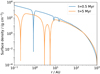 |
Fig. 1 Gas surface density with α = 5 × 10⁻⁴ at time t = 0.5 Myr (blue) and t = 5 Myr (orange) including three planets (setup name V5P123). |
2.4 Migration
The angular momentum exchange with the gas affects the planet’s orbit and can lead to inward or outward migration. The code uses prescriptions for type I and type II migration and interpolates linearly between both cases. Type II is fully reached after opening a deep gap (fgap < 0.1).
For type I migration, the code includes the Lindblad-torque ΓL, corotation-torque ΓC (Paardekooper et al. 2010, 2011), thermal-torque ΓT (Lega et al. 2014; Benítez-Llambay et al. 2015; Masset 2017; Baumann & Bitsch 2020) and the dynamical-torque (Paardekooper 2014; Pierens 2015) for gap opening planets. We calculated the Lindblad-torque and the corotation-torque using Eqs. (3), (52) and (53) of Paardekooper et al. (2011). The thermal-torque is given by Eq. (146) of Masset (2017) and mostly affects small fast accreting planets (Baumann & Bitsch 2020). Their sum yields the total torque without the dynamical scaling.
![Mathematical equation: $\[\Gamma_{\text {tot }}=\Gamma_{\mathrm{L}}+\Gamma_{\mathrm{C}}+\Gamma_{\mathrm{T}}\]$](/articles/aa/full_html/2024/11/aa49840-24/aa49840-24-eq12.png) (7)
(7)
The final Type I torque including the dynamical torque is then given by Eq. (33) of Paardekooper (2014). Those models need the logarithmic gradient of the surface density ![Mathematical equation: $\[\alpha_{\Sigma}=-\frac{\mathrm{d} \ln \Sigma}{\mathrm{~d} \ln r}\]$](/articles/aa/full_html/2024/11/aa49840-24/aa49840-24-eq13.png) . Previously, this value was computed by linear interpolation between gap edges. However, when dealing with multiple gaps, defining the gap edges is less clear. For simplicity, we used the initial disc profile to calculate this gradient. In the beginning, the surface density profile does not change fast, especially at low viscosity. Given that planets open gaps relatively quickly and transition into type II migration, this approximation is adequate.
. Previously, this value was computed by linear interpolation between gap edges. However, when dealing with multiple gaps, defining the gap edges is less clear. For simplicity, we used the initial disc profile to calculate this gradient. In the beginning, the surface density profile does not change fast, especially at low viscosity. Given that planets open gaps relatively quickly and transition into type II migration, this approximation is adequate.
The type II migration occurs on the viscous timescale of the disc ![Mathematical equation: $\[\tau_\nu=a_{\mathrm{p}}^2 / \nu\]$](/articles/aa/full_html/2024/11/aa49840-24/aa49840-24-eq14.png) (Lin & Papaloizou 1986). However, this underestimates the migration time scale for planets, that are more massive than the disc just outside the gap (Baruteau et al. 2014). Therefore the type II migration timescale τII was scaled by a factor relating the planet mass to the disc mass just outside the gap. The full type II migration timescale is given by
(Lin & Papaloizou 1986). However, this underestimates the migration time scale for planets, that are more massive than the disc just outside the gap (Baruteau et al. 2014). Therefore the type II migration timescale τII was scaled by a factor relating the planet mass to the disc mass just outside the gap. The full type II migration timescale is given by
![Mathematical equation: $\[\tau_{\mathrm{II}}=\tau_\nu \times \max \left(1, \frac{M_{\mathrm{p}}}{4 \pi \Sigma_0 a_{\mathrm{p}}^2}\right),\]$](/articles/aa/full_html/2024/11/aa49840-24/aa49840-24-eq15.png) (8)
(8)
with Mp being the planet’s mass and ∑0 and the surface density at the outer gap edge. We determined this value by a vanishing gradient in the surface density. Previously this value was estimated by interpolating the surface density between the gap edges. The previous approach leads to slightly faster migration for very high-mass planets.
Gravitational interaction can lead to orbital resonance between planets resulting in a different migration. For simplicity, we did not use an N-body solver but instead modelled resonance by constraining the migration at certain resonant period ratios. This primarily impacts the relative migration of planets, and we discuss how it influences our results. We only considered the first and most often observed (Winn & Fabrycky 2015) resonance case (2–1). This means the ratio of orbital frequencies is given by Ωin/Ωout = 2 of an inner and outer planet. In addition to the ratio of the frequencies the resonance argument θ which is given by:
![Mathematical equation: $\[\theta=2 ~\Omega_{\text {out }} t+\Omega_{\text {in }} t,\]$](/articles/aa/full_html/2024/11/aa49840-24/aa49840-24-eq16.png) (9)
(9)
needs to stay constant or at least oscillate around a constant angle over time t (Armitage 2013). However, it would require at least 2D calculations to solve this problem exactly. By assuming circular Keplerian orbits and that planets resonate once they reach the 2–1 frequency ratios one can derive a condition for the semi-major axis of two planets. The frequencies are given by the Kepler frequency ΩK at any distance r to a star of mass M* which translates to a semi-major axis ratio of two planets in resonance (θ = 0)
![Mathematical equation: $\[0=2 a_{\mathrm{out}}^{-3 / 2}-a_{\mathrm{in}}^{-3 / 2}\]$](/articles/aa/full_html/2024/11/aa49840-24/aa49840-24-eq17.png) (10)
(10)
![Mathematical equation: $\[\Rightarrow \frac{a_{\text {out }}}{a_{\text {in }}}=2^{2 / 3} \approx 1.58740105\]$](/articles/aa/full_html/2024/11/aa49840-24/aa49840-24-eq18.png) (11)
(11)
We assumed that once a planet crosses the resonant semi-major axis of another planet, both are captured in resonance. They remain in resonance and migrate according to the inner planet’s migration rate. While this approach is a simplification it serves our purpose of studying how multiple planets influence the disc and atmosphere composition.
2.5 Initial conditions
To study the influence of multiple planets on the inner disc’s water abundance we prepared a set of simulations that vary in the number of planetary seeds (from zero to three) and we considered three different disc viscosities with α = 1, 5 and 10 × 10−4, which we call low, mid and high viscosity respectively. The planets started on one out of three initial positions with ap,0 = 3, 20 and 50 AU. We call the planet that starts at 3 AU Planet 1, the planet starting at 20 AU Planet 2, and the planet starting at 50 AU Planet 3. Table 2 gives an overview of the different simulations and Table 1 lists parameters that did not change between the setups.
3 Results
3.1 Disc water content
First, we study the water vapour fraction inside the water ice line. Fig. 2 shows the water surface density in the gas phase relative to the total gas surface density as a function of the radius (x-axis) and the time (y-axis) normalised by the initial fraction. For every viscosity, we show the case of no planet, one, two, and three planets and every combination of two planets. The simulations without planets are consistent with the results of Schneider & Bitsch (2021a). The water content depends on the delivery of icy pebbles and the viscous gas transport.
The evaporation of volatile-rich pebbles causes a density enhancement at evaporation fronts, leading to enhanced inward diffusion of material compared to a purely viscous evolution. Water vapour is transported on a viscous timescale when the water fraction is distributed uniformly. Because we solve Eq. (2) independently for every species, we find the water vapour velocity to be slower than the H & He gas by a factor of ~1/2 at low viscosity after ~1 Myr. Further discussion on the velocity and transport of the water can be found in Appendix B.
At low viscosity, just outside the water ice line, the particle size is limited by fragmentation for ~1 Myr (see Fig. A.1). In this case due to the larger pebble sizes the transport of water-rich solids is very efficient. This increases the pebble flux across the ice line. In comparison, in the case of low viscosity the gas transport is slow. Therefore, the high water fraction in the gas is retained for a longer time.
Increasing the α-viscosity value affects the viscous transport of gas, as well as the drag and size of pebbles. Pebbles are generally smaller and slower at higher viscosity resulting in a lower ice transport towards the ice line. The viscous transport is more efficient and moves water-rich gas faster towards the star. Therefore the excess in the water fraction (compared to the initial fraction) does not persist for more than t ~ 2 Myr in the high viscosity case.
Placing Planet 1 starting at 3 AU (black line in Fig. 2) in the low viscosity disc shows how the water enrichment is lower before the planet crosses the ice line. Especially just before the crossing, the water fraction decreases below the initial value, because the planet blocks water-rich pebbles once it reaches a sufficient mass to open up a deep gap. However, the pebbles pile up outside of the planet-induced gap and as soon as the planet migrates over the water ice line, such that the outer gap edge of the planet is inside the water ice line, all the water-rich pebbles can evaporate relatively quickly. This causes the water fraction to increase to very high values in a relatively short period. After this burst of water vapour, the water vapour is carried away by viscous transport, resulting in a water-poor inner disc a few Myr after the planet has crossed the water ice line. Planet 2 and Planet 3 do not cross the water ice line and block pebbles further outside, lowering the water fraction below the initial value. This effect is smaller when the planet is located further away from the ice line.
For the cases with Planet 1 and at least one other planet the late evolution of the disc from ~8 Myr onwards is sensitive to a second planet that does not cross the ice line. Its presence reduces the water fraction at the end of the disc’s lifetime by an order of magnitude. With a smaller orbit of the second planet (i.e. having Planet 2 instead of Planet 3) the enrichment is more reduced. However, the cases of having only Planet 2 and Planet 2 & Planet 3 are very similar.
As the viscosity increases, the planets can migrate faster. The effect of Planet 1 on the water fraction for the mid and high-viscosity disc is very small. It crosses the ice line early such that it can neither block the pebbles with a gap nor accrete a lot of water-rich pebbles.
However, at mid-viscosity, Planet 2 blocks the pebbles before crossing the ice line around 6 Myr. We thus observe the same pattern as for the innermost planet (Planet 1) in the low viscosity case: the inner disc experiences an outburst of water vapour due to the evaporation of pebbles that are trapped by the migrating planet. Planet 3, in this case, does not cross the water ice line and consequently only blocks the water-rich pebbles, clearly to sub-stellar water abundance in the disc after 2 Myr.
In the case of Planet 1 in combination with Planet 2, we find that the migration of Planet 2 is affected by Planet 1 because the surface density is lower when two planets are present in the disc lowering the value of ∑0 for Planet 2. This increases the migration time scale as given by Eq. (8) compared to the case when only Planet 2 is present. In the setup that includes Planets 2 abd Planet 3 the migration of both planets is slower as they open up an overlapping gap and migrate in resonance (not shown in Fig. 2). In our prescription, this leads to slower migration because the surface density just outside of Planet 2’s gap is significantly lower. Therefore there is no late enrichment with water as Planet 2 never crosses the ice line. With all three planets, the water content in the inner disc rapidly decreases to very low values due to the efficient blocking of water-rich pebbles in the outer disc.
For the high viscosity case, all planets migrate enough to cross the water ice line. This leads to multiple short periods of water enrichment due to the evaporation of blocked pebbles. Except with only Planet 1, the enrichment follows the pattern without a planet because Planet 1 crosses the water ice line during the early pebble enrichment phase. The overall depletion of water inside the water ice line is delayed until the last planet crosses the water ice line. In our setups, this prolongs the time the disc contains high fractions of water to about 3.5 Myr for setups including Planet 3 compared to 2 Myr for the disc-only setup. However, all the setups have similar water fractions after about 4 Myr i.e. after the last planet crossed the ice line and trapped pebbles evaporated.
Fig. 3 shows the total mass fraction of water vapour within the ice line normalised by the initial value. We note the y-axis has different limits for the three different viscosities and the highest enrichment can be observed for the lowest viscosity. The amount of water vapour enrichment depends on the pebble flux, their size, and the gas drift velocity as described above. Again we observe the initial phase of enrichment (within the first 1–4 Myr depending on the viscosity) where planets are relatively small, and the phase of water enrichment every time a planet crosses the water ice line. The disc with no planets shows the largest initial water content because no planets are present that can reduce the inward flux of pebbles. Depending on the distance of a planet to the ice line the enrichment is reduced. The closest planet can reduce the water effect by 50% while the most distant planet has only a small effect.
Focusing on the low viscosity, there is almost no difference between the cases of e.g. Planet 1 alone and Planet 1 & Planet 2. The innermost planet has always the strongest effect. However, for the second peak, which is caused by Planet 1 crossing the ice line there is a clear distinction between no other planet and a second or third planet. The other planets affect the available solid material that can evaporate at this later secondary phase. In the configuration involving only Planet 1, the enrichment is about 70 times above the initial water vapour mass while for the configuration with Planet 1 & Planet 3 it is ~60 and for Planet 1 & Planet 2 ~40. We note the configuration with all planets does not deviate from the configuration with only Planet 1 & Planet 2. Hence a second planet can reduce the ice line crossing-induced water enrichment of the gas by a factor of up to 50%.
For the mid- and high-viscosity, not only the peak amount of water mass is reduced but also the differences between the setups decrease. Nevertheless, the secondary peaks caused by planets crossing the ice line remain more sensitive to the presence of outer planets. Also, Planet 1 migrates relatively quickly inside the water ice line such that its effect on the water mass inside the ice line is small and mostly changes the shape of the initial enrichment peak. In the high-viscosity case, the initial peak of water enrichment is the smallest, as discussed above. Interestingly, once the first planet starts to migrate interior of the water ice line, the peak of water enrichment is similar to the initial peak without any planet.
In principle, the effect of gaps depends on many parameters such as gap location, depth, and viscosity, which in our case depend on the evolving planet properties. Nevertheless, our results in Fig. 3 are similar to previous studies (Kalyaan et al. 2023). Namely, the amount of enrichment strongly depends on the innermost gap (or planet in our case) outside the water ice line. The main difference to the previous study originates from the gap evolution, which in our case depends on the changing planet properties.
Simulation parameters, that don’t change between setups.
Initial setup overview.
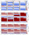 |
Fig. 2 Water fraction in the gas surface density normalised to the initial fraction for α = 1, 5,and 10 × 10−4 from top to bottom. The black lines represent the migration paths of planets. The grey area shades the region exterior to the water ice line. Only some plots show the path of planets because depending on the setup either no planets are present or they remain outside of 2 AU. |
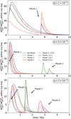 |
Fig. 3 Water mass fraction within the ice line (i.e. integrated over the region with a radius smaller or equal to the position of the water ice line) normalised by the initial value against time. The panels from top to bottom show the three disc viscosities. We note that for α = 1 × 10⁻³ the x-axis only spans to t = 5 Myr, but the late evolution does not deviate from zero which can also be seen in Fig. 2. The colours correspond to different simulation cases, and arrows indicate which planet causes the water vapour to increase by crossing the water ice line. |
3.2 Disc C/O ratio
In this section, we investigate how the disc’s C/O ratio is affected by pebble drift and evaporation in the presence of multiple growing planets. Fig. 4 shows the C/O number ratio normalised to the stellar value. Additionally, the bulk C/O ratio of the atmosphere of the growing planet(s) is shown with a thick line enclosed by two black lines. The colour scale representing the C/O ratio is the same for the disc and the planet.
The most significant oxygen enrichment compared to carbon originates from water, explaining the similarities in the inner region to Fig. 2. The highest ratio of carbon is reached between the evaporation fronts of CO2 and CH4. The available solid material from CH4 is 25% of all carbon species (see Table E.1), which can significantly increase the C/O ratio while CO2 decreases it again. In our chemical model, CO2 only makes up 10% of all carbon species. Planets that accumulate substantial gas from the region between the ice lines of CH4 and CO2 can increase their atmospheric C/O ratio. However, blocking pebbles in this region doesn’t change the C/O ratio in the disc.
The plot shows how the atmosphere C/O changes when a planet crosses an evaporation front. For example, at low viscosity, the atmospheric C/O ratio rapidly decreases after Planet 1 crosses the water ice line. However, for Planet 2 the increase of the C/O ratio in its atmosphere occurs on a much longer timescale despite staying in a high C/O ratio part of the disc. For Planet 1 which ends up having a sub-stellar C/O ratio the effect of an outer planet is observable due to the blockage of water-rich pebbles.
We note that the final C/O ratio in the disc depends on the initial chemical partitioning model. For example, lower methane fractions reduce the C/O ratio between the CO2 and CH4 evaporation fronts and thus also change planetary compositions (e.g. Schneider & Bitsch 2021b).
3.3 Bulk atmosphere composition
Below we investigate if the bulk atmospheric composition of C, O, N and the C/O ratio is altered when multiple planets are present. Fig. 5 shows the final abundances of those elements (relative to hydrogen) normalised by the solar value. Planet 1 is represented by a dot, Planet 2 by a triangle and Planet 3 by a star. To make it comparable with Fig. 3 we used the same colours for the same setups. In the following, we compare the abundances of the multi-planet cases to the single-planet case. The exact numbers can be found in Table D.1.
3.3.1 Low viscosity
In the low-viscosity case, all planets have super-solar carbon abundances. The carbon abundance in the atmosphere of Planet 1 is reduced by ~20% if Planet 2 is present due to the blockage of CO2 and CH4 rich pebbles. Planet 3 decreases the carbon abundance in the atmosphere of Planet 1 by ~10%. If all planets are present, the carbon abundance of the atmosphere of Planet 1 is reduced by ~25%.
The carbon abundance of Planet 3 cannot be explained by the blocking of pebbles because no other planet could alter the chemical composition of the surrounding gas of Planet 3. However, Planet 3 can grow more massive when Planet 2 is present, because of a higher disc accretion rate, which limits the late gas accretion of Planet 3. In addition, the opening of the gap by Planet 2 pushes more gas towards Planet 3. Similar effects have been observed in 2D hydrodynamic simulations (Bergez-Casalou et al. 2023), where an outer planet can accrete gas slightly more efficiently with an inner companion, especially at lower viscosities. Hence Planet 3’s carbon-rich primordial atmosphere is more diluted with low carbon-enriched gas when Planet 2 is present (see Menv/M in Table D.1).
The oxygen abundance in the atmosphere of Planet 1 strongly depends on the amount of accreted water. In the presence of Planet 2 (Planet 3), the abundance of oxygen in Planet 1 is reduced by ~55% (~20%). The oxygen reduction is primarily controlled by Planet 2, and having more planets in the disc has a negligible effect on the carbon abundance. This, unsurprisingly, indicates that the closer planet is more important for the evolution of the final atmospheric abundances than planets further away.
The sub-solar oxygen abundance in the atmosphere of Planet 2 is caused by its position relative to the oxygen-bearing molecules. Planet 2 is far away from the CO evaporation front but also does not cross the CO2 evaporation front. We find that pebble blocking by Planet 3 changes the oxygen abundance in the atmosphere of Planet 2 by ~20%. The difference in the inferred atmospheric composition of Planet 3 is not related to blocked pebbles but to a higher atmosphere mass as explained above.
The abundance of nitrogen in the atmosphere of Planet 1 depends on the blocking of NH3 rich pebbles. Planet 2 and Planet 3 reduce the nitrogen abundance in the atmosphere of Planet 1 by about ~25% and ~10%, respectively. The N2 containing pebbles are located far out in the disc where the viscous timescale is too long to transport N2 enriched gas to planets closer to the star (see Fig. C.1).
The atmosphere of Planet 3 built during the pebble accretion phase has a low nitrogen abundance because only small amounts of NH3-rich pebbles were accreted. As soon as the planet accretes gas, which is heavily enriched by N2, the bulk value for N/H approaches that of the surrounding disc independent of the atmosphere mass. We note that in every simulation N/H is found to be super-stellar due to the very volatile nature of the nitrogen components. Similar to O/H, the N/H ratio of Planet 2 is slightly lower compared to Planet 1 and Planet 3, due to its special position: far interior of the N2 evaporation front, but exterior to the NH3 evaporation front.
The C/O ratio in the atmosphere of Planet 1 is governed by the accretion of water and CO2. These species are blocked by Planet 2 such that the C/O ratio in the atmosphere of Planet 1 is increased by ~75%. Although Planet 3 can block the same species and additionally some methane, Planet 2 dominates the C/O ratio change. The C/O ratio in the atmosphere of Planet 2 is increased by ~10% when Planet 1 or Planet 3 is present, and by ~15% when both planets are included. Some of this change is linked to the difference in the envelope mass fraction. The C/O ratio in the atmosphere of Planet 3 depends on both, the ratio in the solids as well as in the gas. A significant mass of the planet’s envelope is a result of pebble accretion. Our simulations indicate that at low viscosity, super-stellar C/O ratios typically correspond to the middle planet, which is located in a region where water is in icy form, but most carbon-bearing species are already evaporated. This allows the planet to accrete gas with a high C/O ratio, see Fig. 4.
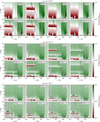 |
Fig. 4 Number ratio of carbon and oxygen (C/O) in the gas phase normalised by the stellar value. The panels from top to bottom show the different disc viscosities α = 1,5, and 10 × 10−4. The coloured line (enclosed between two black lines for visibility reasons) shows the position of the planet and the current bulk C/O number ratio in the atmosphere normalised by the stellar value. |
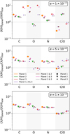 |
Fig. 5 Chemical abundance in the atmosphere at t = 10 Myr and different disc viscosities α = 1, 5 and 10 × 10−4 (top to bottom). The different colours show the different configurations and the different markers show the given planet. The markers for the single planet cases are larger. For the elements C, O, and N the abundances are given in the number ratio to hydrogen normalised by the stellar value while C/O is computed using (C/H)/(O/H) normalised by the stellar value. For the exact numbers see Table D.1. |
3.3.2 Mid viscosity
For the mid-viscosity case, we have similar trends as in the low-viscosity case for the atmosphere of Planet 1. The carbon abundance is reduced by ~30% when Planet 2 is present, by ~15% if Planet 3 is present, and by ~35% when both planets are present. The carbon abundance in the atmosphere of Planet 2 changes slightly because of deviations in the migration. We find that for Planet 3 the carbon abundance in the atmosphere is unchanged.
For Planet 1 the oxygen abundance in the atmosphere strongly depends on the presence of other planets as they can reduce oxygen by ~50% when all the three planets are present. When only one planet is present the reduction is of the order of ~30% (Planet 2) and ~20% (Planet 3). Blocking oxygen-rich ice pebbles depends on both outer planets because the presence of Planet 3 determines whether Planet 2 crosses the water ice line (see Fig. 4). This explains the large difference in the oxygen abundance in the atmosphere of Planet 2 with a reduction of ~65% in the presence of Planet 3. As we discussed earlier, this reduction is not due to blocked pebbles.
Nitrogen is reduced in the atmosphere of Planet 1, Planet 2 and Planet 3 by ~15%, ~25%, and ~10%, respectively. The reduction is most significant in the atmosphere of Planet 2 because Planet 3 can block NH3 rich pebbles. However, in all the cases the atmospheric nitrogen abundance is found to be super-stellar.
The C/O ratio in the atmosphere of Planet 1 is very high with an increase of ~32% if all planets are present. As discussed previously, this can be caused by the blocking of water-rich pebbles. Planet 2 and Planet 3 individually increase the C/O ratio in the atmosphere of Planet 1 by only ~10%. The biggest change in the C/O ratio with an increase by more than 100% can be seen in the atmosphere of Planet 2 because Planet 2 does not cross the water ice line if Planet 3 is present. Unlike in the low viscosity case, Planet 3 can also have a large super-stellar C/O ratio in its atmosphere if it migrates inward without crossing the water ice line. This suggests that the migration history of planets has a crucial effect on the final atmospheric composition.
3.3.3 High viscosity
The migration timescale strongly depends on the viscosity, especially in the late evolution when migration matches the viscous time scale. The migration paths slightly deviate between the setups but all planets migrate relatively fast inwards and line up according to the orbital resonance given by Eq. (10). Therefore the blocking of pebbles is most important for the innermost evaporation lines, namely, of the carbon grains, iron oxides (relatively low abundance), and water. The atmosphere of Planet 1 is less enriched by ~15% in carbon and oxygen. In the atmosphere of Planet 2, the carbon and oxygen abundances are reduced by up to ~10% and ~20%, respectively. The deviations in the atmosphere of Planet 3 are less than ~5% for carbon and less than ~15% for oxygen. The nitrogen abundance in the atmosphere is consistently super-stellar and changes less than ~5% for Planet 1, less than ~20% for Planet 2, and less than ~5% for Planet 3. For the C/O ratio in the atmosphere, the deviations are lower than ~5% for Planet 1, ~15% for Planet 2, and ~10% for Planet 3.
4 Caveats
Our model is rather simple since it is based on modelling disc dynamics using a 1D semi-analytical prescription and a simple two-layer planet model. Therefore, some of our results may change when considering more sophisticated simulations.
First, the planet structure is assumed to be a simple core plus envelope, and therefore claims in our study about the bulk composition may not be observable in planets that have more complex structures such as composition gradients (e.g. Vazan & Helled 2020) or an interplay between the atmosphere and interiors. In addition, in reality, the planetary bulk composition could change after formation via several processes such as atmospheric escape and giant impacts (e.g. Genda & Abe 2004; Guillot et al. 2022). Atmospheric escape is not expected to play an important role during the formation phase. When the planet is small, the atmosphere is coupled to the disc and the upper layers of the atmosphere should have similar composition to the disc gas. Also during the detached phase, when the planet is massive enough to open a gap, atmospheric escape is not very likely. This is because when the planet is still surrounded by the disc, the disc shields the atmosphere from high energy radiation of the star. Furthermore, we assume that 10% of the accreted pebbles contribute to the initial atmosphere rather than the core during core formation. This value affects the chemical abundances in a giant atmosphere and it was shown that this ratio strongly depends on the local formation conditions (Valletta & Helled 2020). However, in our case, this mostly changes the results for Planet 3 when it grows to different masses depending on the presence of Planet 2.
Second, we do not calculate the gravitational forces between planets which would affect the mean-motion resonance. Using an N-body integrator would properly account for such interactions and in addition include other mean-motion-resonance frequencies resulting in different spacing of planet pairs and resonant chains. Also, depending on the migration speed, resonant period ratios can be crossed and scattering could occur (Bitsch et al. 2020; Bitsch & Izidoro 2023). However, this affects our results only in the case of multiple planets because, in the case of a single planet, the migration rate is determined solely by the planet-disc interaction. With multiple planets, the different resonant ratios can lead to different configurations; however, the key trends inferred in this work regarding the enrichment are expected to remain.
Third, our simplified gap formation method naturally extends to overlapping gaps by multiplying the individual Gaussian viscosity perturbation. However, this is not based on simulating the gas-planet interaction in a common gap of two planets (e.g. Masset & Snellgrove 2001; Bergez-Casalou et al. 2023). But it is unlikely to affect our conclusions since the exact shape of the gap does not play a role as long as the gap can block pebbles efficiently. However, a more realistic overlapping of gaps can affect the pebble and gas reservoir between planets and may change their accretion (Weber et al. 2018). This could be investigated further in future studies.
Fourth, the disc chemistry is static and molecules cannot be converted into other species. In principle, chemical reactions can change the composition of ice and gas. Studies show that depending on the level of ionisation of the disc the chemical evolution becomes significant after a few 105 yr and settles into a steady state after 7 Myr (Eistrup et al. 2016, 2018). The chemical evolution of pebbles is found to be slower than their drift (Booth & Ilee 2019; Eistrup & Henning 2022), but can become important if the presence of a pressure gap slows down the inward drift. The latter effect is most likely to influence the results of this study. Especially at low viscosity, we see that large amounts of pebbles are blocked outside the planet’s gap and evaporate when the planet crosses an ice line. We suggest that future studies investigate the change in the chemical composition of blocked pebbles. We note that even if chemical reactions take place, the overall abundance is unchanged. If the planet migrates into hotter regions these molecules could be accreted by the planet in the gaseous form. It is therefore critical to determine the physical state of the different elements and the associated chemistry in various conditions as well as determining the accretion rates of gas and solids during planet formation.
Fifth, we assume a fixed starting time of 5 × 10⁴ years for the planetary embryos. Different starting times affect the growth of planets and change the amount of pebbles that pass the planet before a deep gap is formed. Starting at later times leaves more time for pebbles to drift inwards. In this case, the reduction of the initial water enrichment we see in Fig. 3 would be smaller. Also, the late enrichment that occurs after a planet crosses an ice line would be smaller because most pebbles drift away early. However, our choice of the early starting times can be justified due to the following reasons. First, a planetary embryo starting later than ~0.5 Myr is less likely to form a giant (Savvidou & Bitsch 2023). Second, disc substructures indicate an early planet formation (Delussu et al. 2024), although not all gaps are caused by planets (e.g. Tzouvanou et al. 2023). Clearly, it would be interesting to investigate the sensitivity of the results when considering different starting times and we hope to explore this in future research.
Sixth, solving Eq. (2) independently for every gas species assumes there is no angular momentum exchange between the species. This changes gas velocities compared to a case where the gas is fully interacting. A comparison between different disc models that include multiple molecular species and how to correctly model the diffusion of the species can be found in Desch et al. (2017). To justify our model, we show the gas velocity of water vapour relative to the gas velocity of the H & He gas in the Appendix B. For a short time, the water vapour spreads very fast throughout the disc. We can therefore expect that water spreads faster than the viscous time scale because a high composition gradient should lead to fast diffusion through the disc. On the other hand, the water gas velocity is lower than the H & He gas when the water fraction is uniform within the ice line. In that case, we should expect it to be similar to the velocity of the H & He. As shown in Desch et al. (2017) the methods used here tend to overestimate the diffusion through the disc. However, this effect is only relevant during the early disc evolution (t ≲ 1 Myr) and for discs with a low viscosity. Within our model, the change in the atmospheric abundances is significant and qualitative trends should be independent of the exact mechanism of gas transport. However, when trying to explain the chemical composition and formation scenario of a specific planetary system rather than general trends, a self-consistent treatment of the interactions between different species and their angular momentum exchange would be necessary.
Finally, this study did not include planetesimals although planetesimals are expected to exist. For example, planet gaps with pressure bumps can increase planetesimal formation (Eriksson et al. 2021; Sándor et al. 2024) and reduce the inward pebble flux (Danti et al. 2023). In the case of our model, this would reduce the effect of an outer planet, decreasing volatiles in an inner planet’s atmosphere by blocking pebbles although gaps blocking pebbles may be more important than planetesimals locking material in place (Kalyaan et al. 2023). On the other hand, planetesimals can be swept up by an inward-migrating planet (Shibata et al. 2020, 2022) and evaporate at ice lines. Additionally, an inward-migrating planet raises the eccentricities of planetesimals potentially increasing the density of pebbles and dust by ablation and fragmentation (Batygin & Laughlin 2015; Eriksson et al. 2021). Furthermore, planetesimals that form in the pressure bump of a planet can be scattered inwards and ablate due to high eccentricities and gas drag (Eriksson et al. 2021). This would decrease the effect of pebble blocking. Accounting for the effect of planetesimals in future research is clearly desirable.
5 Summary and conclusions
Planetary systems often harbour multiple planets; hence formation models should include planet formation in the context of other companions rather than focusing on a single planet. We used our planet formation model to investigate the influence of multiple planets on the inner disc and planets by blocking pebbles and preventing enrichment of the disc due to pebble evaporation. Therefore we extended the chemcomp code, first presented in Schneider & Bitsch (2021a), to the formation of multiple planets simultaneously.
We showed that gap-opening planets can reduce the water vapour enrichment in the disc. Similar to the study of Kalyaan et al. (2023), we found that the most important effect originates from the innermost planet outside an ice line. A planet close to the water ice line can grow quickly to block water-rich pebbles and decrease the water vapour content of the inner disc. However, the planet is likely to cross the evaporation front, so all the trapped pebbles can evaporate after all resulting in multiple phases of enrichment. The amount of these late enrichment phases depends then on the next planet further out. The amount of this later enrichment phase depends on the next planet outside the evaporation front.
The effect of blocked pebbles is more important at lower viscosities because pebble evaporation-induced enrichment is stronger, gas transport is slower (e.g. Schneider & Bitsch 2021b; Mah et al. 2023) and planet migration is reduced. If planets remain longer in outer regions of the disc they can block more pebbles that otherwise would evaporate. Also, we find that in every simulation there is always an initial phase where enough pebbles drift inwards to alter the chemical composition of the inner disc region before planets grow enough to block pebbles.
The C/O ratio in the disc is mostly affected by the relatively abundant water vapour. We also find, that trapping carbon rich pebbles affects the C/O ratio less than blocking water rich pebbles. In particular, due to the delayed gap opening (caused by the growth of a giant planet), water-rich pebbles can drift inwards and evaporate in all simulations. Therefore, the discs in all our simulations show a phase with a sub-solar C/O ratio inside the water ice line. This implies that young discs (≲1 Myr) with super-solar C/O ratios need to harbour initial pressure perturbations that are not caused by growing planets.
The presence of a gap-opening planet outside the water ice line can reduce the volatile enrichment in the bulk composition of a giant planet’s atmosphere inside the water ice line. In our study, we show that the atmospheric C/H and O/H can be reduced by ~30% and ~50%, respectively, when other planets exist farther out and block volatile-rich pebbles. However, the importance of blocked pebbles depends on the exact scenario, i.e. how planets migrate relative to each other and how they cross the evaporation fronts. Therefore, the viscosity is a key property in our simulations. Yet, the presence of an outer planet generally does not imply that the inner planet has sub-solar C/H or O/H. Overall this effect is less important than expected because large amounts of pebbles can drift inwards relatively early before planets can carve a pebble-blocking gap. Additionally, when planets migrate over evaporation fronts the trapped material evaporates and enriches the gas again, which can be accreted by an inner planet.
In all our simulations the bulk atmospheric abundance of nitrogen was found to be super-solar. We assume that 10% of nitrogen is contained in NH3 and the rest in N2. Because the N2 evaporation front is far out we need to distinguish between two cases. First, the viscous evolution is fast enough to transport N2 gas into the inner disc region. Second, the evolution is too slow. In the first case blocking NH3 rich pebbles can reduce the nitrogen abundance in the atmosphere of close-in planets by ~25%. In contrast, in the second case this reduction is only ~15% because N2 enriched gas can be accreted instead. However, if the outermost planet is initially located beyond the N2 evaporation front, this enrichment can be reduced as well. In both cases, our model implies that exoplanetary atmospheres should have super-stellar nitrogen abundances if pebble drift and evaporation are significant. We note that studies that focused on nitrogen enrichment in Jupiter’s atmosphere suggested that this enrichment could also be a result of core formation near or beyond the N2 ice line (Bosman et al. 2019; Öberg & Wordsworth 2019). However, in our case nitrogen enrichment is not necessarily a result of formation near the N2 ice line making it a more common outcome of planet formation. In any case, we can conclude that nitrogen is an important element in constraining the planetary formation history and hope to address this topic in future research.
Our study suggests that the number of planets can affect the formation scenario of individual planets and plays a crucial role. However, there are improvements to enhance the model that should be made. Additionally, a broader parameter space will give more insight into the complex interplay between multiple growing planets. Further investigations of these topics are required in order to link the atmospheric composition of exoplanets with their formation location.
Acknowledgements
We thank Sho Shibata for the helpful discussion on the effects of planetesimals and Christoph Mordasini for a helpful discussion. ME and RH acknowledge support from SNSF grant 200020_215634. We also thank the referee for the comments that improved the quality of our manuscript.
Appendix A Pebble size limits
We follow the two-population model of Birnstiel et al. (2012) to determine the pebble sizes. The Stokes number St in the Epstein drag regime is given by
![Mathematical equation: $\[\mathrm{St}=\Omega_{\mathrm{K}} \tau_f=\frac{\pi a \rho_{\bullet}}{2 \Sigma_{\mathrm{gas}}},\]$](/articles/aa/full_html/2024/11/aa49840-24/aa49840-24-eq19.png) (A.1)
(A.1)
with τf, a, and ρ• being the friction time, particle size, and density respectively. The pebble size limits can be reformulated in terms of a maximum Stokes number. The drift limit Stdritf, the fragmentation limit Stfrag and the relative drift-induced fragmentation limit Stdf, are given by the equations:
![Mathematical equation: $\[\mathrm{St}_{\mathrm{drift}}=f_{\mathrm{d}} \frac{v_{\mathrm{K}}^2}{\gamma c_{\mathrm{s}}^2} \frac{\Sigma_{\text {dust }}}{\Sigma_{\mathrm{gas}}},\]$](/articles/aa/full_html/2024/11/aa49840-24/aa49840-24-eq20.png) (A.2)
(A.2)
![Mathematical equation: $\[\mathrm{St}_{\mathrm{frag}}=f_{\mathrm{f}} \frac{v_{\mathrm{f}}^2}{3 \alpha c_{\mathrm{s}}^2},\]$](/articles/aa/full_html/2024/11/aa49840-24/aa49840-24-eq21.png) (A.3)
(A.3)
![Mathematical equation: $\[\mathrm{St}_{\mathrm{df}}=\frac{v_{\mathrm{f}} v_{\mathrm{K}}^2}{\gamma c_{\mathrm{s}}^2(1-N)},\]$](/articles/aa/full_html/2024/11/aa49840-24/aa49840-24-eq22.png) (A.4)
(A.4)
with vK = rΩK being the Kepler velocity, ![Mathematical equation: $\[\gamma=\left|\frac{\mathrm{d} \ln P}{\mathrm{~d} \ln r}\right|\]$](/articles/aa/full_html/2024/11/aa49840-24/aa49840-24-eq23.png) the logarithmic pressure gradient, ∑solid the dust surface density, fd = 0.55 and ff = 0.37 fit factors, and N = 0.5 a factor that expresses the size differences of particles that collide due to different drift speeds. In Fig. (A.1) we show the Stokes number of pebbles and the limiting Stokes numbers at different times in the disc. We exclude the drift-induced fragmentation limit from the plot because it’s always higher than the other two limiting processes.
the logarithmic pressure gradient, ∑solid the dust surface density, fd = 0.55 and ff = 0.37 fit factors, and N = 0.5 a factor that expresses the size differences of particles that collide due to different drift speeds. In Fig. (A.1) we show the Stokes number of pebbles and the limiting Stokes numbers at different times in the disc. We exclude the drift-induced fragmentation limit from the plot because it’s always higher than the other two limiting processes.
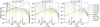 |
Fig. A.1 Stokes Number of pebbles (solid lines), the drift limit (dotted lines) and fragmentation limit (grey dashed line) at different times (colours) for the unperturbed disc. The different viscosities are shown from left to right (setups: V1noP, V5noP & V10noP). Vertical lines show the position of various ice lines. The fragmentation limit is only shown for t = 0.5 Myr because it is almost constant over time. |
The fragmentation limit is almost constant in time because the only changing quantity is cs. We assume a time-independent temperature profile but the mean molecular weight of the gas can change cs. However, the mean molecular weight is dominated by hydrogen and helium and therefore almost constant over time.
For the low viscosity, pebbles just outside the water ice line are limited by fragmentation for t ≲ 1 Myr. So early on, pebbles can grow exponentially to large sizes and enrich the inner disc with high amounts of water. After t ~ 1 Myr pebbles outside the water ice-line become fully drift-limited and smaller over time. For the high viscosity case, fragmentation dominates from the inner disc edge to r ~ 5 AU for as long as t ≲ 4 Myr, resulting in smaller pebbles because the fragmentation limit is inversely proportional to α. The drift limit is only important further out.
Appendix B Water transport
We show the water gas velocity relative to the H & He gas velocity in Fig. (B.1). In our model, each molecular species can have different velocities because we solve Eq. (2) for each species individually. When pebbles evaporate they create a density enhancement in the gas leading to a diffusion of water faster than the viscous time scale of the disc. Hence, the water is very fast initially and quickly increases the water fraction towards the inner edge of the gas disc. The water velocity becomes slower than the velocity of the H & He gas when the water fraction becomes uniform across the inner region of the disc (around t ~ 1 Myr for the low viscosity). Close to the water ice line (within ≲ 0.1 AU from its location) the velocity decreases and gets negative to ensure the conservation of angular momentum within the water vapour. Water vapour is transported outward, where it re-condensates after crossing the ice line. As discussed in the caveats the diffusion of water vapour is overestimated early in the disc. For a comparison between different viscous evolution equations that treat the transport of individual molecular species correctly see Desch et al. (2017).
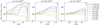 |
Fig. B.1 Velocity of the water vapour relative to the velocity of H & He at different times (colours) for the unperturbed disc. The different viscosities are shown from left to right (setups: V1noP, V5noP & V10noP). The vertical line shows the position of the water ice lines. A positive velocity ratio indicates an inward flow of gas. |
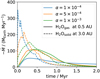 |
Fig. B.2 Disc accretion rate |
![Mathematical equation: $\[\dot{M}\]$](/articles/aa/full_html/2024/11/aa49840-24/aa49840-24-eq24.png)
Fig. (B.2) shows the disc accretion rate ![Mathematical equation: $\[\dot{M}\]$](/articles/aa/full_html/2024/11/aa49840-24/aa49840-24-eq25.png) of water vapour at 0.5 AU (inside the water ice line) and the disc accretion rate of solids at 3 AU (outside the water ice line). Initially, pebble drift carries more water towards the ice line than water vapour is transported away by viscosity. This increases the water fraction of the gas inside the water ice line. With higher viscosity, gas transport is more efficient, quickly reducing this excess water. At low viscosity, the gas transport is slow and the solid accretion rate is high because pebbles are larger. This leads to a high water fraction in the gas disc that persists for a long time. In contrast, at high viscosity, the solid accretion rate increases slower and reaches only ~50% of the low viscosity maximum value. However, gas transport is more efficient, resulting in a lower and shorter-lived increase in the water fraction of the gas disc (see Sec. 3 & Fig. (2)).
of water vapour at 0.5 AU (inside the water ice line) and the disc accretion rate of solids at 3 AU (outside the water ice line). Initially, pebble drift carries more water towards the ice line than water vapour is transported away by viscosity. This increases the water fraction of the gas inside the water ice line. With higher viscosity, gas transport is more efficient, quickly reducing this excess water. At low viscosity, the gas transport is slow and the solid accretion rate is high because pebbles are larger. This leads to a high water fraction in the gas disc that persists for a long time. In contrast, at high viscosity, the solid accretion rate increases slower and reaches only ~50% of the low viscosity maximum value. However, gas transport is more efficient, resulting in a lower and shorter-lived increase in the water fraction of the gas disc (see Sec. 3 & Fig. (2)).
Appendix C Disc nitrogen abundance
We show the N/H ratio normalised by the stellar value of the unperturbed disc in Fig. (C.1). At low viscosity, the nitrogen contained in NH3 rich pebbles increases the abundance to super stellar values in the inner disc regions. The ratio stays high for the entire disc lifetime. Gas enriched by N2 containing pebbles is too slow to reach radii of r ≲ 3 AU within the 10 Myr, making the region outside the methane ice line less enriched for most of the disc’s lifetime. At higher viscosity, N2 enriched gas can reach the inner region within the disc lifetime, similar to methane. Consequently, the whole disc has a super stellar nitrogen abundance for most of the disc’s lifetime.
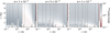 |
Fig. C.1 Gas N/H number ratio normalised to the solar value as a function of time and radius. The three viscosities are shown from left to right (setups: V1noP, V5noP & V10noP). |
Appendix D Final planet composition and mass
Final planet composition and mass.
Appendix E Condensation temperatures and volume mixing ratios
Condensation temperatures and volume mixing ratios (by number).
Appendix F Initial disc composition
Initial disc composition based on solar elemental abundances (Asplund et al. 2009).
References
- Andrews, S. M., Huang, J., Pérez, L. M., et al. 2018, ApJ, 869, L41 [NASA ADS] [CrossRef] [Google Scholar]
- Ansdell, M., Williams, J. P., van der Marel, N., et al. 2016, ApJ, 828, 46 [Google Scholar]
- Armitage, P. J. 2013, Astrophysics of Planet Formation (Cambridge, UK: Cambridge University Press) [Google Scholar]
- Asplund, M., Grevesse, N., Sauval, A. J., & Scott, P. 2009, ARA&A, 47, 481 [NASA ADS] [CrossRef] [Google Scholar]
- Bae, J., Isella, A., Zhu, Z., et al. 2023, Protostars and Planets VII, 534, 423 [NASA ADS] [Google Scholar]
- Baruteau, C., Crida, A., Paardekooper, S. J., et al. 2014, Planet-Disk Interactions and Early Evolution of Planetary Systems, 667 [Google Scholar]
- Batygin, K., & Laughlin, G. 2015, PNAS, 112, 4214 [NASA ADS] [CrossRef] [Google Scholar]
- Baumann, T., & Bitsch, B. 2020, A&A, 637, A11 [NASA ADS] [CrossRef] [EDP Sciences] [Google Scholar]
- Benisty, M., Bae, J., Facchini, S., et al. 2021, ApJ, 916, L2 [NASA ADS] [CrossRef] [Google Scholar]
- Benítez-Llambay, P., Masset, F., Koenigsberger, G., & Szulágyi, J. 2015, Nature, 520, 63 [Google Scholar]
- Bergez-Casalou, C., Bitsch, B., Pierens, A., Crida, A., & Raymond, S. N. 2020, A&A, 643, A133 [NASA ADS] [CrossRef] [EDP Sciences] [Google Scholar]
- Bergez-Casalou, C., Bitsch, B., & Raymond, S. N. 2023, A&A, 669, A129 [NASA ADS] [CrossRef] [EDP Sciences] [Google Scholar]
- Birnstiel, T., Dullemond, C. P., & Brauer, F. 2010, A&A, 513, A79 [NASA ADS] [CrossRef] [EDP Sciences] [Google Scholar]
- Birnstiel, T., Klahr, H., & Ercolano, B. 2012, A&A, 539, A148 [NASA ADS] [CrossRef] [EDP Sciences] [Google Scholar]
- Bitsch, B., & Izidoro, A. 2023, A&A, 674, A178 [NASA ADS] [CrossRef] [EDP Sciences] [Google Scholar]
- Bitsch, B., Morbidelli, A., Johansen, A., et al. 2018, A&A, 612, A30 [NASA ADS] [CrossRef] [EDP Sciences] [Google Scholar]
- Bitsch, B., Izidoro, A., Johansen, A., et al. 2019, A&A, 623, A88 [NASA ADS] [CrossRef] [EDP Sciences] [Google Scholar]
- Bitsch, B., Trifonov, T., & Izidoro, A. 2020, A&A, 643, A66 [EDP Sciences] [Google Scholar]
- Bitsch, B., Schneider, A. D., & Kreidberg, L. 2022, A&A, 665, A138 [NASA ADS] [CrossRef] [EDP Sciences] [Google Scholar]
- Booth, R. A., & Ilee, J. D. 2019, MNRAS, 487, 3998 [CrossRef] [Google Scholar]
- Bosman, A. D., Cridland, A. J., & Miguel, Y. 2019, A&A, 632, L11 [NASA ADS] [CrossRef] [EDP Sciences] [Google Scholar]
- Boss, A. P. 1997, Science, 276, 1836 [Google Scholar]
- Boss, A. P. 1998, ApJ, 503, 923 [Google Scholar]
- Brauer, F., Dullemond, C. P., & Henning, T. 2008, A&A, 480, 859 [NASA ADS] [CrossRef] [EDP Sciences] [Google Scholar]
- Crida, A., & Morbidelli, A. 2007, MNRAS, 377, 1324 [Google Scholar]
- Crida, A., Morbidelli, A., & Masset, F. 2006, Icarus, 181, 587 [Google Scholar]
- Danti, C., Bitsch, B., & Mah, J. 2023, A&A, 679, A7 [CrossRef] [EDP Sciences] [Google Scholar]
- Delussu, L., Birnstiel, T., Miotello, A., et al. 2024, A&A, 688, A81 [NASA ADS] [CrossRef] [EDP Sciences] [Google Scholar]
- Desch, S. J., Estrada, P. R., Kalyaan, A., & Cuzzi, J. N. 2017, ApJ, 840, 86 [NASA ADS] [CrossRef] [Google Scholar]
- Dullemond, C. P., Birnstiel, T., Huang, J., et al. 2018, ApJ, 869, L46 [NASA ADS] [CrossRef] [Google Scholar]
- Eistrup, C., & Henning, T. 2022, A&A, 667, A160 [NASA ADS] [CrossRef] [EDP Sciences] [Google Scholar]
- Eistrup, C., Walsh, C., & van Dishoeck, E. F. 2016, A&A, 595, A83 [NASA ADS] [CrossRef] [EDP Sciences] [Google Scholar]
- Eistrup, C., Walsh, C., & van Dishoeck, E. F. 2018, A&A, 613, A14 [NASA ADS] [CrossRef] [EDP Sciences] [Google Scholar]
- Emsenhuber, A., Mordasini, C., Burn, R., et al. 2021, A&A, 656, A69 [NASA ADS] [CrossRef] [EDP Sciences] [Google Scholar]
- Eriksson, L. E. J., Ronnet, T., & Johansen, A. 2021, A&A, 648, A112 [NASA ADS] [CrossRef] [EDP Sciences] [Google Scholar]
- Garufi, A., Ginski, C., van Holstein, R. G., et al. 2024, A&A, 685, A53 [NASA ADS] [CrossRef] [EDP Sciences] [Google Scholar]
- Genda, H., & Abe, Y. 2004, Lunar and Planetary Science Conference, 1518 [Google Scholar]
- Guillot, T., Fletcher, L. N., Helled, R., et al. 2022, arXiv e-prints [arXiv:2205.04100] [Google Scholar]
- Gundlach, B., & Blum, J. 2015, ApJ, 798, 34 [Google Scholar]
- Ikoma, M., Nakazawa, K., & Emori, H. 2000, ApJ, 537, 1013 [NASA ADS] [CrossRef] [Google Scholar]
- Izidoro, A., Bitsch, B., Raymond, S. N., et al. 2021, A&A, 650, A152 [EDP Sciences] [Google Scholar]
- Johansen, A., & Lambrechts, M. 2017, Annu. Rev. Earth Planet. Sci., 45, 359 [Google Scholar]
- Kalyaan, A., Pinilla, P., Krijt, S., et al. 2023, ApJ, 954, 66 [NASA ADS] [CrossRef] [Google Scholar]
- Keppler, M., Benisty, M., Müller, A., et al. 2018, A&A, 617, A44 [NASA ADS] [CrossRef] [EDP Sciences] [Google Scholar]
- Knierim, H., Shibata, S., & Helled, R. 2022, A&A, 665, A5 [Google Scholar]
- Lambrechts, M., & Johansen, A. 2012, A&A, 544, A32 [NASA ADS] [CrossRef] [EDP Sciences] [Google Scholar]
- Lambrechts, M., Johansen, A., & Morbidelli, A. 2014, A&A, 572, A35 [NASA ADS] [CrossRef] [EDP Sciences] [Google Scholar]
- Lega, E., Crida, A., Bitsch, B., & Morbidelli, A. 2014, MNRAS, 440, 683 [Google Scholar]
- Lin, D. N. C., & Papaloizou, J. 1986, ApJ, 309, 846 [Google Scholar]
- Lodato, G., Scardoni, C. E., Manara, C. F., & Testi, L. 2017, MNRAS, 472, 4700 [NASA ADS] [CrossRef] [Google Scholar]
- Lodders, K. 2003, ApJ, 591, 1220 [Google Scholar]
- Lynden-Bell, D., & Pringle, J. E. 1974, MNRAS, 168, 603 [Google Scholar]
- Machida, M. N., Kokubo, E., Inutsuka, S.-I., & Matsumoto, T. 2010, MNRAS, 405, 1227 [Google Scholar]
- Mah, J., Bitsch, B., Pascucci, I., & Henning, T. 2023, A&A, 677, A7 [Google Scholar]
- Masset, F. S. 2017, MNRAS, 472, 4204 [NASA ADS] [CrossRef] [Google Scholar]
- Masset, F., & Snellgrove, M. 2001, MNRAS, 320, L55 [Google Scholar]
- Matsumura, S., Brasser, R., & Ida, S. 2021, A&A, 650, A116 [NASA ADS] [CrossRef] [EDP Sciences] [Google Scholar]
- Mayor, M., Marmier, M., Lovis, C., et al. 2011, arXiv e-prints [arXiv:1109.2497] [Google Scholar]
- Morbidelli, A., Lambrechts, M., Jacobson, S., & Bitsch, B. 2015, Icarus, 258, 418 [NASA ADS] [CrossRef] [Google Scholar]
- Mollière, P., Molyarova, T., Bitsch, B., et al. 2022, ApJ, 934, 74 [CrossRef] [Google Scholar]
- Müller, A., Keppler, M., Henning, T., et al. 2018, A&A, 617, A2 [Google Scholar]
- Öberg, K. I., & Wordsworth, R. 2019, AJ, 158, 194 [Google Scholar]
- Ormel, C. W., & Klahr, H. H. 2010, A&A, 520, A43 [NASA ADS] [CrossRef] [EDP Sciences] [Google Scholar]
- Paardekooper, S. J. 2014, MNRAS, 444, 2031 [NASA ADS] [CrossRef] [Google Scholar]
- Paardekooper, S. J., Baruteau, C., Crida, A., & Kley, W. 2010, MNRAS, 401, 1950 [NASA ADS] [CrossRef] [Google Scholar]
- Paardekooper, S.-J., Baruteau, C., & Kley, W. 2011, MNRAS, 410, 293 [NASA ADS] [CrossRef] [Google Scholar]
- Pierens, A. 2015, MNRAS, 454, 2003 [NASA ADS] [CrossRef] [Google Scholar]
- Pinilla, P., Lenz, C. T., & Stammler, S. M. 2021, A&A, 645, A70 [NASA ADS] [CrossRef] [EDP Sciences] [Google Scholar]
- Pollack, J. B., Hubickyj, O., Bodenheimer, P., et al. 1996, Icarus, 124, 62 [NASA ADS] [CrossRef] [Google Scholar]
- Rosenthal, L. J., Knutson, H. A., Chachan, Y., et al. 2022, ApJS, 262, 1 [Google Scholar]
- Sándor, Z., Guilera, O. M., Regály, Z., & Lyra, W. 2024, A&A, 686, A78 [NASA ADS] [CrossRef] [EDP Sciences] [Google Scholar]
- Savvidou, S., & Bitsch, B. 2023, A&A, 679, A42 [NASA ADS] [CrossRef] [EDP Sciences] [Google Scholar]
- Schneider, A. D., & Bitsch, B. 2021a, A&A, 654, A71 [Google Scholar]
- Schneider, A. D., & Bitsch, B. 2021b, A&A, 654, A72 [NASA ADS] [CrossRef] [EDP Sciences] [Google Scholar]
- Schneider, A. D., & Bitsch, B. 2023, arXiv e-prints [arXiv:2401.15686] [Google Scholar]
- Shakura, N. I., & Sunyaev, R. A. 1973, A&A, 24, 337 [NASA ADS] [Google Scholar]
- Shibata, S., Helled, R., & Ikoma, M. 2020, A&A, 633, A33 [NASA ADS] [CrossRef] [EDP Sciences] [Google Scholar]
- Shibata, S., Helled, R., & Ikoma, M. 2022, A&A, 659, A28 [NASA ADS] [CrossRef] [EDP Sciences] [Google Scholar]
- Tzouvanou, A., Bitsch, B., & Pichierri, G. 2023, A&A, 677, A82 [NASA ADS] [CrossRef] [EDP Sciences] [Google Scholar]
- Valletta, C., & Helled, R. 2020, ApJ, 900, 133 [NASA ADS] [CrossRef] [Google Scholar]
- Vazan, A., & Helled, R. 2020, A&A, 633, A50 [NASA ADS] [CrossRef] [EDP Sciences] [Google Scholar]
- Weber, P., Benítez-Llambay, P., Gressel, O., Krapp, L., & Pessah, M. E. 2018, ApJ, 854, 153 [NASA ADS] [CrossRef] [Google Scholar]
- Weidenschilling, S. J. 1977, MNRAS, 180, 57 [Google Scholar]
- Winn, J. N., & Fabrycky, D. C. 2015, ARA&A, 53, 409 [Google Scholar]
All Tables
Initial disc composition based on solar elemental abundances (Asplund et al. 2009).
All Figures
|
Fig. 1 Gas surface density with α = 5 × 10⁻⁴ at time t = 0.5 Myr (blue) and t = 5 Myr (orange) including three planets (setup name V5P123). |
| In the text | |
|
Fig. 2 Water fraction in the gas surface density normalised to the initial fraction for α = 1, 5,and 10 × 10−4 from top to bottom. The black lines represent the migration paths of planets. The grey area shades the region exterior to the water ice line. Only some plots show the path of planets because depending on the setup either no planets are present or they remain outside of 2 AU. |
| In the text | |
|
Fig. 3 Water mass fraction within the ice line (i.e. integrated over the region with a radius smaller or equal to the position of the water ice line) normalised by the initial value against time. The panels from top to bottom show the three disc viscosities. We note that for α = 1 × 10⁻³ the x-axis only spans to t = 5 Myr, but the late evolution does not deviate from zero which can also be seen in Fig. 2. The colours correspond to different simulation cases, and arrows indicate which planet causes the water vapour to increase by crossing the water ice line. |
| In the text | |
|
Fig. 4 Number ratio of carbon and oxygen (C/O) in the gas phase normalised by the stellar value. The panels from top to bottom show the different disc viscosities α = 1,5, and 10 × 10−4. The coloured line (enclosed between two black lines for visibility reasons) shows the position of the planet and the current bulk C/O number ratio in the atmosphere normalised by the stellar value. |
| In the text | |
|
Fig. 5 Chemical abundance in the atmosphere at t = 10 Myr and different disc viscosities α = 1, 5 and 10 × 10−4 (top to bottom). The different colours show the different configurations and the different markers show the given planet. The markers for the single planet cases are larger. For the elements C, O, and N the abundances are given in the number ratio to hydrogen normalised by the stellar value while C/O is computed using (C/H)/(O/H) normalised by the stellar value. For the exact numbers see Table D.1. |
| In the text | |
|
Fig. A.1 Stokes Number of pebbles (solid lines), the drift limit (dotted lines) and fragmentation limit (grey dashed line) at different times (colours) for the unperturbed disc. The different viscosities are shown from left to right (setups: V1noP, V5noP & V10noP). Vertical lines show the position of various ice lines. The fragmentation limit is only shown for t = 0.5 Myr because it is almost constant over time. |
| In the text | |
|
Fig. B.1 Velocity of the water vapour relative to the velocity of H & He at different times (colours) for the unperturbed disc. The different viscosities are shown from left to right (setups: V1noP, V5noP & V10noP). The vertical line shows the position of the water ice lines. A positive velocity ratio indicates an inward flow of gas. |
| In the text | |
|
Fig. B.2 Disc accretion rate |
| In the text | |
|
Fig. C.1 Gas N/H number ratio normalised to the solar value as a function of time and radius. The three viscosities are shown from left to right (setups: V1noP, V5noP & V10noP). |
| In the text | |
Current usage metrics show cumulative count of Article Views (full-text article views including HTML views, PDF and ePub downloads, according to the available data) and Abstracts Views on Vision4Press platform.
Data correspond to usage on the plateform after 2015. The current usage metrics is available 48-96 hours after online publication and is updated daily on week days.
Initial download of the metrics may take a while.