| Issue |
A&A
Volume 691, November 2024
|
|
|---|---|---|
| Article Number | A357 | |
| Number of page(s) | 19 | |
| Section | Extragalactic astronomy | |
| DOI | https://doi.org/10.1051/0004-6361/202449244 | |
| Published online | 26 November 2024 | |
Modelling absorption and emission profiles from accretion disc winds with WINE
1
INAF – Istituto di Astrofisica e Planetologia Spaziali, Via del Fosso del Caveliere 100, I-00133 Roma, Italy
2
INAF – Osservatorio Astronomico di Roma, Via Frascati 33, 00078 Monteporzio, Italy
3
Dept. of Physics, University of Rome “Tor Vergata”, Via della Ricerca Scientifica 1, 00133 Rome, Italy
4
INFN – Roma Tor Vergata, Via Della Ricerca Scientifica 1, 00133 Rome, Italy
5
INAF – Osservatorio Astronomico di Trieste, Via G. B. Tiepolo 11, 34143 Trieste, Italy
6
IFPU – Institute for Fundamental Physics of the Universe, Via Beirut 2, 34014 Trieste, Italy
⋆ Corresponding author; This email address is being protected from spambots. You need JavaScript enabled to view it.
Received:
16
January
2024
Accepted:
10
October
2024
Abstract
Context. Fast and massive winds are ubiquitously observed in the UV and X-ray spectra of active galactic nuclei (AGNs) and other accretion-powered sources. Several theoretical and observational pieces of evidence suggest they are launched at accretion disc scales, carrying significant mass and angular momentum. Thanks to such high-energy output, they may play an important role in transferring the energy released by accretion to the surrounding environment. In the case of AGNs, this process can help to set the so-called co-evolution between an AGN and its host galaxy, which mutually regulates their growth across cosmic time. To precisely assess the effective role of UV and X-ray winds at accretion disc scales, it is necessary to accurately measure their properties, including mass and energy rates. However, this is a challenging task, due to both the limited signal-to-noise ratio of available observations and the limitations of the models currently used in the spectral analysis.
Aims. We aim to maximise the scientific return of current and future observations by improving the theoretical modelling of these winds through our Winds in the Ionised Nuclear Environment (WINE) model. WINE is a spectroscopic model specifically designed for disc winds in AGNs and compact accreting sources, which couples photoionisation and radiative transfer with special relativistic effects and a three-dimensional model of the emission profiles.
Methods. We explore with WINE the main spectral features associated with the disc winds in AGNs, with a particular emphasis on the detectability of the wind emission in the total transmitted spectrum. We explore the impact of the wind ionisation, column density, velocity field, and geometry in shaping the emission profiles. We simulated observations with the X-ray microcalorimeter Resolve on board the recently launched XRISM satellite and the X-IFU on board the future Athena mission. This allows us to assess the capabilities of these telescopes in the study of disc winds in X-ray spectra of AGNs for the typical physical properties and exposure times of the sources included in the XRISM performance verification phase.
Results. The wind kinematic and geometry (together with the ionisation and column density) deeply affect both shape and strength of the wind spectral features. Thanks to this, both Resolve and, on a longer timescale, X-IFU will be able to accurately constrain the main properties of disc winds over a broad range of ionisation, column densities, and covering factors. We also investigate the impact of the spectral energy distribution (SED) on the resulting appearance of the wind. Our findings reveal a dramatic difference in the gas opacity when using a soft, Narrow Line Seyfert 1-like SED compared to a canonical powerlaw SED with a spectral index of Γ ≈ 2.
Key words: accretion / accretion disks / line: profiles / galaxies: active / quasars: absorption lines / quasars: emission lines / quasars: supermassive black holes
© The Authors 2024
 Open Access article, published by EDP Sciences, under the terms of the Creative Commons Attribution License (https://creativecommons.org/licenses/by/4.0), which permits unrestricted use, distribution, and reproduction in any medium, provided the original work is properly cited.
This article is published in open access under the Subscribe to Open model. This email address is being protected from spambots. You need JavaScript enabled to view it. to support open access publication.
1. Introduction
Disc winds are ubiquitously observed in many accreting sources, from compact sources to stellar and super massive black holes at the centre of Active Galactic Nuclei (AGNs). AGN-driven winds are considered to be one of the fundamental mechanisms in shaping the accretion process itself and the interaction with the surrounding host environment. Indeed, for AGNs, winds are regarded as one of the key players in the feedback towards the host galaxy (see e.g. Faucher-Giguère & Quataert 2012; King & Pounds 2015; Fiore et al. 2017; Torrey et al. 2020 and references therein).
Given the high degree of ionisation displayed by the gas, most of the observable transitions fall in the UV and X-ray bands. By comparing the observed spectra with simulated ones, it is possible to constrain the wind properties, first of all NH, vout, ξ; that is, the column density, outflow velocity, and ionisation degree. The latter quantity is defined as the ratio between the ionising luminosity, Lion (i.e. the luminosity above the ionisation threshold of hydrogen, E = 13.6 eV) and the product between the gas density and distance: ξ = Lion/nr2 Tarter et al. (1969). In the UV range, most of the observed features are classified as Broad Absorption Lines (BALs), traced by mildly ionised lines such as CIV, NV, and Si IV with velocities from a thousand km s−1 up to 0.3 c, being c the speed of light (see e.g. Murray et al. 1995; Arav et al. 2001; Bruni et al. 2019; Bischetti et al. 2022; Vietri et al. 2022). In the X-ray band, the two broad classes into which winds are commonly classified are Warm Absorbers (WAs, observed in ∼50% of AGNs, Blustin et al. 2005; Piconcelli et al. 2005), in which the ionisation status is roughly consistent with the ions giving rise to BALs, i.e. −1 ≲ log(ξ/erg cm s−1)≲3 and NH ≲ 1023 cm−2, and higher-ionisation, mildly relativistic Ultra-Fast Outflows (UFOs), with log(ξ/erg cm s−1)≳3, NH > 1023 cm−2 and vout around 0.1 c, with a high-velocity tail until 0.3 c (see e.g. Pounds et al. 2003; Cappi et al. 2009; Fiore et al. 2017; Laha et al. 2021; Luminari et al. 2021; Chartas et al. 2021; Matzeu et al. 2023 and refs. therein). It is important to note that, most of these winds being spatially unresolved, line-of-sight integrated spectroscopy is the prime tool to study them.
From the above spectral quantities, estimates of the wind energetics, namely the mass and energy fluxes, are usually estimated under the assumption of spherical symmetry and classic (i.e. non-relativistic) dynamics as (see e.g. Crenshaw & Kraemer 2012; Tombesi et al. 2012)
 (1)
(1)
where r0, Cf are the wind launching radius and covering factor, respectively, and μ, mp are the mean atomic mass per proton and the proton mass (see Krongold et al. 2007; Fiore et al. 2024 for alternative formulations).
Several photoionisation codes are available to fit the observed spectra, such as Cloudy (Ferland et al. 2017), XSTAR (Kallman et al. 2021), and SPEX (Kaastra et al. 1996). For a given incident’s Spectral Energy Distribution (SED), NH, ξ, they allow one to compute the ionisation balance of the gas and obtain both the transmitted and emitted spectra, which can then be fitted to the observations. These codes allow for an extensive exploration of the parameter space of disc winds and robust estimates of their energetics, and thus readily allow one to assess the wind role and dynamics. However, it must be noted that such codes are designed to be as universal as possible, allowing them to reproduce virtually any astrophysical setting, from the atmospheres of stars to diffuse Lyα nebulae. Their physical picture is therefore not able to account for the full complexity of the disc wind phenomenon, which shows peculiar properties, such as strong velocity gradients, mildly relativistic velocities, and a non-spherical geometry, strongly deviating from the spherical symmetry. Such features can largely affect the gas spectroscopic appearance, and thus must be properly accounted for to obtain reliable synthetic wind spectra and to constrain the wind properties meaningfully. Specifically, we note three major assumptions of present photoionisation codes that are not met by disc winds:
-
The gas is at rest with respect to the luminosity source (i.e. zero net velocity).
-
The thermal motion of the gas regulates the line broadening (i.e. gas velocity shearing is negligible).
-
The gas cloud is spherically symmetric around the radiation source, resulting in emission profiles with Gaussian shapes1.
Together with the signal-to-noise and resolving power limitations of current X-ray spectra, such theoretical assumptions often prevent a reliable estimate of both the wind covering fraction, Cf (which is usually assumed by looking at the statistical recurrence of outflows in large samples), and r0, which is estimated through indirect arguments; that is, by equating vout with the escape velocity or through the definition of ξ and assuming a constant wind density and a plane-parallel geometry (see e.g. Tombesi et al. 2011 and discussion in Laurenti et al. 2021). As a result, the derived ̇Mout, ̇Eout usually have order-of-magnitude uncertainties, which prevent a detailed assessment of the feedback of such outflows on both the accretion process and the host environment (see e.g. Figs. 2 and 3 in Tombesi et al. 2012 and Fig. 8 in Smith et al. 2019).
Of particular interest are the so-called P-Cygni profiles, where, in analogy with the stellar atmospheres (Castor & Lamers 1979), a line transition is detected both in emission and absorption, with the latter at slightly blueshifted (i.e. higher) energies due to the bulk motion of the absorbing gas along the line of sight (LOS). Under the hypothesis that these spectral components are produced in the same expanding gas, such a remarkable spectral feature allows one to probe both the outflowing gas along our LOS and its distribution over the solid angle. This clearly represents a great advantage for measuring physical and dynamical properties of the gas with respect to spectra where only absorption lines are detected. Notable examples of P-Cygni profiles associated with UFOs in AGNs have been discovered in the X-ray spectra of PDS 456 (Nardini et al. 2015; Luminari et al. 2018), 1H 0707-495 (Hagino et al. 2016), PG1448+273 (Kosec et al. 2020; Laurenti et al. 2021) and I Zwicky 1 (Reeves & Braito 2019). However, in most of the observations it is difficult to statistically rule out a non-negligible contribution by the accretion disc reflection to the emission profile (see e.g. Parker et al. 2017; Middei et al. 2023), as is discussed in detail by Parker et al. (2022) through sets of dedicated X-ray simulations. Updated, more accurate disc wind models are therefore needed to shed light on this intriguing aspect of disc winds and the interplay of their spectroscopy imprint with further emission components not related to the wind, especially given the unprecedented resolving power offered by the microcalorimeter Resolve onboard XRISM (Tashiro et al. 2020) and Athena’s X-IFU (Barret & Cappi 2019; Barret et al. 2023).
To address the limitations discussed above and get a more accurate description of disc winds, we developed the Wind in the Ionised Nuclear Environment (WINE) spectroscopic model. WINE features accurate photoionisation balance and radiative transfer through the XSTAR code and a detailed modelling of the dynamics and geometry of disc winds from compact sources and accreting black holes. Its main features are the inclusion of special relativity in both gas absorption and emission, a detailed treatment of the wind density and velocity profiles, and a proper representation of the wind geometry, in order to deal with the assumptions listed above. The result is a physically motivated modelling of the wind emission and absorption profiles, which allows one to self-consistently constrain the main wind properties and energetics. A description of the Monte Carlo approach is outlined in Luminari et al. (2018) (where it is also applied to the X-ray UFO in the quasar PDS 456), while special relativity effects are discussed in Luminari et al. (2020), Marzi et al. (2023) and applications of WINE to the UFOs in the AGNs PG1448+273 and NGC 2992 are presented in Laurenti et al. (2021); Luminari et al. (2023a), respectively.
The structure of this paper is as follows. In Sect. 2, we illustrate the structure of WINE and its free parameters, and we show characteristic WINE-generated spectra in Sect. 3. Then, we investigate the detectability of the emission profiles for typical UFO parameters, both through an algorithm that scans the wind spectra (Sect. 4) and through simulated observations with the Resolve microcalorimeter on board XRISM (Sect. 5) and the AthenaX-IFU (Sect. 6). Finally, we discuss and summarise our results in Sect. 7.
We note that in the following we focus on the typical parameter range of WAs and UFOs in AGNs, but WINE is perfectly suitable for the study of any kind of disc wind arising from compact sources. Hereafter, ξ, NH will be expressed in units of erg cm s−1 and cm−2, respectively, and we shall omit them for ease of reading.
2. The working scheme of WINE
We designed WINE as a self-consistent model for disc winds, able to directly probe the main properties of the intervening gas – ionisation, velocity, column density, radial location, and geometry – and thus to reliably estimate its energetics. We tuned the number of free parameters to the (expected) constraining power of the microcalorimeter Resolve on board the XRISM satellite, but we shall also discuss possible avenues for further improvements.
For a given geometry and dynamics of the wind (which are set by the input parameters), the gas column density is sliced into a series of geometrically thin shells. Photoionisation computation starts from the innermost shell and is then propagated outwards. The resulting quantities – the transmitted spectrum and gas emissivity – are processed to compute the wind absorption and emission profiles as a function of the physical properties of the wind (velocity, opening angles, LOS, etc.). As we shall discuss in detail below, a number of input parameters regulate the ionisation structure of the gas, while others regulate the kinematics and the geometry, and thus the observational appearance of the gas spectral features.
2.1. Wind geometry and dynamics
We assume a biconical geometry for the wind (see Fig. 1), centred on the accreting source (represented as a black dot) and with the same symmetry axis as the accretion disc (assumed to be planar). We assume that the wind is directed radially outwards (but see Appendix A for further discussion on this) and we consider the rear cone to be obscured by the disc (in yellow). The luminosity source is point-like and located at the centre (blue region in Fig. 1). The wind is enclosed by an initial and final radius, r0, r1, and has an inner and outer opening angle, θin and θout, respectively (shown in red and green in Fig. 1), while the inclination of the LOS, i, is shown in light grey. The geometry is in line with most of the observations and models of accretion disc wind in the literature (Proga et al. 2000; Proga & Kallman 2004; Krongold et al. 2007; Ohsuga et al. 2009; Fukumura et al. 2010; Hagino et al. 2015; Matthews et al. 2016; Maksym et al. 2023). Moreover, galactic-scale outflows also show quasi-spherical or biconical morphologies (Rupke & Veilleux 2013; Feruglio et al. 2015; Venturi et al. 2018; Mingozzi et al. 2019; Menci et al. 2019, 2023).
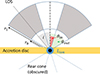 |
Fig. 1. Geometry of the WINE model. The shaded grey area indicates the wind volume. θin, θout represents the wind inner and outer opening angle with respect to the symmetry axis (vertical dotted line). The LOS has an inclination angle, i, with respect to the axis. The accretion disc is represented with a yellow bar, and the black and blue dots indicate, respectively, the accreting and the luminosity sources, which are assumed to be point-like. Finally, r0, r1 indicate the wind’s initial and final radius, respectively. |
According to this geometry, the wind covering factor, Cf, is
 (2)
(2)
The inner cavity, specified by θin, can also be interpreted as a first-order parametrisation for (possible) density variations along the polar angle. Such variations are indeed expected for both radiative and magnetohydrodynamic (MHD) accelerations, which produce variable wind distributions in the equatorial and poloidal directions. As an example, for magnetically driven winds, the interplay between poloidal and toroidal magnetic fields may lead to a collimated, relativistic jet-like outflow around the rotation axis and a smooth, mildly relativistic outflow outside the jet region (Fukumura et al. 2010, 2014; Yuan et al. 2015; Cui & Yuan 2020). In this case, we expect the jet region to lie in the 0 < θ < θin interval, and the wind in the θin < θ < θout one. Simulations of radiatively driven winds instead suggest that most of the wind develops closer to the equatorial region, while the polar one is associated with failed winds due to overionisation by the central luminosity source (Proga & Kallman 2004; Higginbottom et al. 2014). Moreover, a configuration with θin ≈ θout is able to reproduce a funnel-shaped wind; such a structure is foreseen by several theoretical models (see e.g. Elvis 2000; Matthews 2016; Matthews et al. 2020; Sim et al. 2008, 2010a,b) with the aim of unifying most of the outflowing structures observed in the optical/UV and X-ray bands; that is, from the broad- and narrow-line regions up to UFOs.
The gas density and velocity are parametrised as powerlaw functions of the radial coordinate of the cone, r, as follows:
 (3)
(3)
 (4)
(4)
where n0 ≡ n(r = r0),v0 ≡ v(r = r0). Several analytical calculations point towards such powerlaw trends (see e.g. Faucher-Giguère & Quataert 2012; Menci et al. 2019) in the case of a fast wind expanding in a perturbation-free environment. Specifically, in the case of momentum- and energy-conserving flows, the following relations hold (Faucher-Giguère & Quataert 2012):
 (5)
(5)
so it is possible to link the velocity profile to the density one. We have focussed on an ‘ideal’ (perturbation-free) outflow, since we expect strong inhomogeneities to be suppressed at typical disc wind scales. Even though an intrinsic degree of anisotropy in the gas properties – density, temperature – is naturally expected at the outflow launching point, the strong acceleration gradients and the extreme velocities, which make the gas trans- to super-sonic (see e.g. Proga et al. 2000; Cui & Yuan 2020; Yamamoto & Fukue 2021), are expected to quench the growth of physical gradients and the setting of multi-phase flows. The development of a fully inhomogeneus flow – that is, δρ/⟨ρ⟩≳1, δT/⟨T⟩≳1 (where δρ = |ρ − ⟨ρ⟩| and ⟨ρ⟩ is the average density and the same holds for the temperature, T) – is typically expected at WA and BLR scales. The theoretical picture, however, is not yet fully established, and we refer to Dannen et al. (2020), Waters et al. (2021, 2022) and references therein for further discussions.
We performed a first-order radiative transfer to account for the absorption of the gas emission spectrum by the gas column itself. As is discussed in Sect. 3.3, such absorption is negligible for typical UFO ionisation degrees and velocities, but it becomes appreciable for a higher gas opacity; that is, low ionisation and higher column densities, log(ξ)≤3, NH ≥ 1023.
2.2. Input parameters
The parameters regulating photoionisation and radiative transfer (via the XSTAR code) are the following:
-
Lion, SI, the incident luminosity and spectrum, respectively (either tabulated or analytic).
-
ξ0, the ionisation parameter at the inner face of the gas cloud.
-
v0, αv, the starting velocity and the index in Eq. (4). αv can also be linked to α using the relations of Eq. (5).
-
NHmax, the total column density of the wind, and the linear or logarithmic stepping pace.
-
r0, the initial radius of the wind.
-
α, the index of the density profile in Eq. (3).
-
vturb, the gas turbulent velocity. This can be either set by the user directly or computed self-consistently by the code following Eq. (8) below.
Metallicity is a free parameter and hereafter we adopt the standard solar values of Sanders et al. (1968); in other words, the default XSTAR ones. Once photoionisation computation is performed, the transmitted spectrum and the line emissivities are used to obtain the wind absorption and emission spectrum. The line profiles are a function of the wind geometry and dynamics, which is set by the following free parameters (see Fig. 1):
-
v0, αv, the velocity profile (see above).
-
r0, the launching radius (see above).
-
θout, the opening angle of the wind cone.
-
i, the inclination of the LOS with respect to the symmetry axis of the cone.
-
θin, the opening angle of the inner wind cavity.
For practical purposes, when computing tables of absorption and emission spectra it is possible to let WINE iterate over ranges of input values.
2.3. Ionisation and radiative transfer
The wind ionisation and radiative transfer is computed in WINE through a multi-layer approach with repeated calls to an ionisation code, similarly to what has already been done in previous works, such as Schurch & Done (2007), Fukumura et al. (2010), Saez & Chartas (2011). For a given NH, the wind is divided into M linear(or log)-spaced slabs, each one with a column density, δNHm. For a given set of input parameters, photoionisation computation is started from the first shell using XSTAR and then propagated outwards up to the M-th shell. This slicing allows one to implement the wind velocity and density profiles of Eqs. (3), (4) and to build absorption and emission templates for increasing NH. The shell thickness, δNHm (or, equivalently, M), is a free parameter and has to be tuned so that the variation in n, r, log(ξ) within each shell is negligible. In all of the cases presented in this paper, we find that δNHm = 1023cm−2 allows one to optimally sample the wind column.
For a given ξ0, r0, the initial density of the wind, n0, is determined by inverting the definition of ξ0:
 (6)
(6)
and the final radius of the wind, r1, is computed as a function of NHmax:
 (7)
(7)
For each m-th slab, the program analytically calculates all the input quantities needed to perform a relativistically corrected photoionisation run. In the following, we first describe the procedure for m = 1 and then we generalise it for m > 1 slabs. WINE sets NH = δNH1 and Lion, SI, ξ0, n0, α according to the values provided by the user. The slab’s initial radius is r1i = r0, while the final radius, r1f, is a function of δNH1 through Eq. (7). We define a column density-averaged slab velocity, vavg, as  , where ravg is the radius enclosing half of the slab column density, δNH/2 = ∫r1ir1avgn(r)dr. The procedure described in Luminari et al. (2020) is implemented to account for the special relativity effects in radiative transfer due to the bulk motion of the gas. Finally, vturb is defined as
 (8)
(8)
where δv = |v(r1i)−v(r1avg)| represents the variation in v(r) within the slab, while σint = 0.1 ⋅ v(ravg) and accounts for the intrinsic turbulence of the outflow. Given that here we focus on the study of the fastest wind components, we set a lower limit to σint equal to 3000 km s−1, in order to match the typical turbulence detected in the more distant (and perhaps less turbulent) broad-line region clouds (Kollatschny et al. 2012). Moreover, such a lower limit is also consistent with what is observed for UFOs (see e.g. Tombesi et al. 2011; Gofford et al. 2013. However, σint is a free parameter in WINE and can be changed by the user. The r0 run returns the (relativistic-corrected) transmitted spectrum from the first slab, corresponding to a column density of NH = δNH and, separately, the wind line emissivities (see below for more details).
To calculate the radiative transfer for the second slab, the transmitted spectrum from the first slab, ST, 1, is given as the input incident spectrum. Accordingly, the initial radius of the slab corresponds to the final radius of the previous slab – r2i = r1f – and the final radius, r2f, is calculated in the same way as r1f. r0 is run using  , where LT, 1 is the luminosity of ST, 1. vavg and vturb are updated accordingly. This procedure is iterated over the M slabs, up to NHmax, and the absorption spectra up to NHmax are computed.
2.4. Wind emission
In r0 and in most of the current codes (see Sect. 1), the gas emission is computed assuming null outflow velocity and a spherically symmetric geometry around the central luminosity source. In order to go beyond such assumptions, WINE models the emission profile via a Monte Carlo approach as a function of the wind kinematics and the geometry, adopting the same multi-layer structure used to compute the transmitted spectrum.
For each slab, the code uses the r0-computed line emissivities, ζ, which are in units of erg s−1 cm−3 and represent a ‘luminosity density’ for a given transition within the slab. The emission spectrum of the m-th slab is calculated according to the following steps:
-
The volume of the slab, Vs, is determined as a function of its geometry; that is, rmi, rmf, θout, θin.
-
The slab is populated with a high number, K, of points, whose coordinates are randomly assigned with a Monte Carlo method inside Vs2.
-
For each k-th point (where k ∈ [1, K]):
-
An average volume δV = Vs/K is assigned, and the luminosity, Zi, of the i − th transition is calculated as Zi = ζi ⋅ δV, where i ∈ [0, I].
-
Using special relativity formulae, the line energy, Ei, and luminosity, Zi, are projected along the LOS according to so-called ‘relativistic beaming’, which is described as (Luminari et al. 2020)
 (9)
(9)where
 , vavg represents the column density-averaged slab velocity and θ is the angle between the LOS and the coordinates of the k-th point.
-
-
The combination of EiLOS, ZiLOS from all the lines (i.e. from i = 0 to =I) gives the emitted spectrum of the k-th point.
-
The sum of the spectra from k = 0 to K produces the slab emission spectrum.
Finally, the composition of the slab emission spectra for increasing m gives the wind emission spectrum for increasing column density, up to NHmax. To account for the self-absorption of such an emission spectrum by the gas, at each m-th slab the radiation emitted by the inner slabs is absorbed according to the opacity, τ, of the present slab. Such an opacity is computed as the ratio between the transmitted and the incident spectrum of that slab, accounting for relativistic effects as in Sect. 2.3. Moreover, we introduce a volume filling factor, Cv, so that only a fraction, 0 ≤ Cv ≤ 1, of the incoming emission is absorbed. We illustrate some examples in Sect. 3.3. The physical scenario of WINE is that of a single-phase gas column, and thus Cv = 1 would be expected. However, we allow for lower values to account for possible inhomogeneities, including clumpiness, which would allow part of the emitted spectrum to escape the wind unattenuated. In the highest signal-to-noise spectra, Cv could be directly fitted through to the spectroscopic imprint of the self-absorption on the emission profiles (see Figs. 5 and 6). More generally, hints as to the degree of inhomogeneity of the gas can also be obtained indirectly; for example, if the best-fit values of the wind absorption and emission are different, suggesting different properties along the LOS with respect to the whole emitting region, or in case of temporary obscuring winds (such as those seen in NGC 5548 or MR 2251, Kaastra et al. 2014; Mao et al. 2022) due to denser clumps embedded in the intervening gas.
3. Wind spectra
3.1. Input spectral energy distribution and wind parameter space
In this section, we show some results obtained with WINE regarding the absorption and emission features emerging from an ionised gas with a range of physical properties. We consider the UV-to-X-ray SED of a well-studied Narrow-Line Seyfert 1 galaxy (NLSy1, Komossa 2008; Tarchi et al. 2011; Rakshit et al. 2017), I Zwicky 1, which can be considered to be a representative highly accreting AGN showing a UFO-related P-Cygni feature in its X-ray spectrum (Reeves & Braito 2019; hereafter RB19). As is reported in RB19 and shown in Fig. 2 for clarity, the UV-to-X-ray spectrum is parametrised as a series of broken powerlaws with a peak in the far-UV regime and is built from previous FUSE (Moos et al. 2000; Sahnow et al. 2000) observations and the 2015 datasets from OM and EPIC instruments on board XMM–Newton (Jansen et al. 2001; Mason et al. 2001; Strüder et al. 2001; Turner et al. 2001). It consists of a powerlaw with a photon index of Γ = 1.75 below 12.5 eV and a second one with Γ = 2.2 up to 300 eV. Between 300 eV and 1.2 keV, Γ = 3.3 to approximate the strong observed soft excess, while Γ = 2.2 above 1.2 keV. The black hole mass and the 2–10 keV luminosity reported in RB19 are MBH = 2.8 ⋅ 107 M⊙, L2 − 10 = 5 ⋅ 1043ergs−1, implying λEdd ≈ 0.85. For simplicity, we set a flat gas density profile (i.e. α = 0 in Eq. (3)). We set the launching radius to a fiducial value of r0 = 50rG (see discussion in Luminari et al. 2021) and vturb according to Eq. (8). Here and in the following section, we span the typical parameter space of X-ray UFOs; that is, NH ∈ [1022, 1024],v0 ∈ [0, 0.3]c, log(ξ0)∈[3, 5]. We consider a momentum-conserving wind and, consequently, we set the velocity index, αv = (2 − α)/2. We set vturb to the (fiducial) lower limit of 3000 km/s to reduce the smearing and to better investigate the wind absorption and emission lines. Finally, we fixed θin = 0 for simplicity.
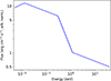 |
Fig. 2. UV-to-X-ray SED of the NLSy1 I Zwicky 1. |
According to these initial conditions, the wind is in a geometrically thin configuration and the scaling of v, ξ with r is limited, so it is possible to clearly appreciate the role of the different parameters. A useful quantity to characterise the wind geometrical thickness as a function of NH is  ; that is, the difference between the radius enclosing a column density, NH, and the initial radius, r0, normalised by r0. According to the density profile, α, Δr can be expressed as
 (10)
(10)
where r0, g ≡ r0/rG is the launching radius in gravitational units. For α = 0, Δr can be written as
 (11)
(11)
where we put λion ≡ Lion/LEdd = 0.85, as for I Zwicky 1. In this formula, we omitted special relativity effects for simplicity (see Luminari et al. 2023a for more details). The variation in ionisation and velocity along the wind column can be expressed as
 (12)
(12)
 (13)
(13)
so that ξ(r)≈ξ0, v(r)≈v0 in the whole parameter space probed in this paper, confirming the negligible variation in the wind properties along the LOS.
3.2. Absorption profiles
The top panel of Fig. 3 shows the absorption spectrum for v0 = 0.05, 0.10, 0.30c and NH = 1023, log(ξ0) = 4. The strongest absorption profiles are due to the Lyα, Lyβ lines of Fe XXIV and XXV, which are the most abundant Fe ions at such ionisation (Kallman et al. 2004). Due to special relativity effects, for increasing outflow velocities, absorption lines are both blueshifted and have lower equivalent widths, as is discussed in Luminari et al. (2020). Moreover, the turbulent velocity, vturb, increases for increasing v0 (following Eq. (8)) and strongly modifies the absorption profiles, blending together the Lyα lines of Fe XXV and XXVI for v0 = 0.30 c at energies around 9 keV.
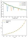 |
Fig. 3. Impact of the relativistic effects on the asorption features. Top: Absorption profiles for v0 = 0.00, 0.10, 0.30c (colour coding, see legend) and NH = 1023, log(ξ0) = 4 in the rest-frame spectrum between 6–10 keV. For increasing v0, absorption lines are increasingly blueshifted and show lower EWs, as was expected from special relativity effects. Bottom: Ratio, Ψrel, between intrinsic and observed gas opacity as a function of the gas velocity, v (in units of c). |
Due to the relativistic effects, when inferring the column density of the gas from its measured opacity in observed spectra, it is necessary to include a correction to get the intrinsic gas opacity and then the intrinsic NH. The bottom panel of Figure 3 shows the ratio, Ψrel, between intrinsic and observed opacity as a function of the gas velocity, v (in units of c), computed with WINE (blue diamonds), assuming v is parallel to r for simplicity. This relation is found to be well described by the following equation:
 (14)
(14)
which can be used to derive the intrinsic NH from the NH obtained from the measured (i.e. apparent) opacity.
3.3. Emission profiles
Fig. 4 shows the emission profiles for log(ξ0) = 3, v0 = 0.1c, NH = 1023 for different wind geometries. According to Eq. (9), the projected velocity, vproj, can be expressed as  , where θ is the angle between the LOS and the gas velocity (which depends on θout, θin, i, see Fig. 1). When θ = 0 deg – that is, when the gas is directed radially outwards and vout is parallel to the LOS – vproj is the highest,
  , while when the velocity is opposed to the LOS – that is, θ = 180 deg – vproj is the lowest,
  .
.
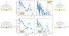 |
Fig. 4. Emission profiles for different wind geometries, assuming log(ξ0) = 3, v0 = 0.10c, NH = 1023. Top row: Wind seen ‘face on’ (i = 0) and θout = 90, 30 deg (left and right panel, respectively). Bottom row: ‘Edge-on’ winds (i = 90 deg) and θout = 90, 30 (left and right panel, respectively). For comparison, the i = 0, θout = 90 deg case is reported with light grey lines in all the panels. |
In the top left panel, we show the case for θout = 90 deg, i = 0: the transmitted flux is maximised, since the emitting volume is the largest possible, as is shown in the cartoon (i.e. a hemisphere filling the solid angle above the accretion disc) and the LOS coincides with the symmetry axis, resulting in a beamed emission towards the observer (see Eq. (9)). The accretion disc is thus seen ‘face on’ and θ ranges from 0 to 90 deg.
The emission profile is the combination of the lines due to several ions, with the strongest ones originating from the transitions with the highest oscillator strengths for the most abundant ions. We highlight with vertical dashed lines the rest-frame wavelength of some of them; from left to right, they are due to Mg XXII, Si XIII, Si XIII, Si XIV, S XV, Ar XVII, Ca XIX, Fe XXII, and Ni XXIV. The emission lines extend bluewards of their rest-frame energies, spanning a range of projected velocities from  (for the gas at θ = 90deg) to
  (θ = 0deg).
In the top right panel of Fig. 4, we have set the cone opening angle θout = 30 deg and we have kept the inclination i = 0. The emitted luminosity is lower than that found in the previous case (plotted again with grey lines for comparison) and the low-energy (low-velocity) side of each emission peak is reduced, since there is no gas at 30deg < θout < 90 deg. In the θout = 90, i = 90 deg case (bottom left panel of Fig. 4), the accretion disc is instead seen ‘edge on’, and then θ ranges from 0 to 180 deg. As a consequence, the spectral features are broadened over a larger energy interval than in the ‘face on’ case, since they are projected over an increased velocity space. Finally, for θout = 30, i = 90 deg (bottom right panel), the emission region is outside the LOS and θ ranges from 60 to 120 deg. This explains the lower vproj and the overall decrease in the transmitted flux, since the relativistic beaming reduces the radiation projected along the LOS.
Wind emission spectra for log(ξ0) = 3 and 4 are shown in Figs. 5 and 6, respectively. In both figures, the top and bottom panels are for v0 = 0.0 and 0.1 c, while in all cases θout = 90, i = 0 deg, NH = 1024. Orange(red) lines indicate the emission profiles for Cv = 0( = 1) and pink(purple) lines the composition of such spectrum with the absorption one. For reference, absorption spectra are reported with dashed black lines. For increasing v0, the gas cross section decreases due to relativistic effects and emission features are spread over a larger observed energy interval. As a consequence of both these effects, the emitted flux per unit energy is lower for increasing v0. As we shall show in Sect. 4, this will have important implications for the detectability of emission features in the total (i.e. emission+absorption) wind spectrum. By comparing Figs. 5 and 6, it can be seen that the higher gas ionisation directly translates into lower gas opacity. For log(ξ0) = 4, the strongest transitions in the hard X-ray band (E > 5 keV) are those of Fe XXV Kα and Kβ (E = 6.7, 7.8 keV, respectively) and Fe XXVI Kα (E = 6.9 keV). The attenuation of the emitted radiation by the gas self-absorption is mostly effective, both for high gas opacity and for low velocity. The latter effect is due to the fact that absorption and emission lines are closer in the velocity space, and thus the weakening of the emerging emission is maximised. The narrow absorption features at rest-frame energies of E = 7–8 keV and, for log(ξ) = 3, also between E = 3–5 keV, are due to resonances of the photoelectric cross-section of several abundant elements, most notably iron (Kallman et al. 2004), which are not convolved for the gas turbulent velocity in XSTAR (T. Kallman, priv. comm.). The high gas opacity for log(ξ) = 3, NH = 5 ⋅ 1023 leads to strong absorption and emission in the soft band (E < 5 keV), virtually leading to a complete absorption of the incident continuum.
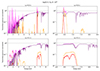 |
Fig. 5. WINE spectrum for log(ξ0) = 3, NH = 5 ⋅ 1023 and v0 = 0.0, 0.1 c (top and bottom row, respectively). The left panels show the E = 1–8.5 keV spectrum, while the right panels zoom in above E = 6 keV. Orange(red) lines represent the emission spectrum and pink(purple) the total (absorption + emission) spectrum for Cv = 0(1). The absorption spectrum is shown with dashed black lines. For ease of visualisation, the spectra are divided by the incident continuum. |
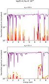 |
Fig. 6. WINE spectrum for log(ξ0) = 4, NH = 5 ⋅ 1023 and v0 = 0.0, 0.1 c (top and bottom panel, respectively). The colour coding is as in Fig. 5. |
4. Wind emission detectability
We explored the disc wind parameter space to evaluate the strength of the emission features in the wind spectrum. Starting from the input parameters presented in Sect. 3, we simulated with WINE a range of column densities, NH ∈ [5, 20]⋅1023, for log(ξ0)≥3, in order to optimally sample the properties of the P-Cygni profiles observed in UFOs (see Sect. 1). We set θout = 90 deg, θin = 0, i = 0deg in order to maximise the wind emission, and CV = 1, as is suggested by such high-covering factor geometry. We set an energy resolution of 5 eV as a fiducial reference value for the Resolve microcalorimeter on board XRISM.
We defined the emission as detectable if the flux of the emission spectrum were higher than the absorption one in at least two adjacent energy bins. We selected two energy bands of interest, a soft band from 0.5 to 2.5 keV and a hard band between 5 and 10 keV. Figure 7 shows the median equivalent width (mEW) of the emission features, derived by the following procedure. We scanned the soft and hard energy bands looking for intervals of two or more bins satisfying the detectability requirement. For each interval, we computed the EW of the emitted spectrum with respect to the transmitted one. Finally, we calculated the median value of the distribution of EWs for all the intervals. We have focussed on mEW, rather than the total EW, since we are primarily interested in the detectability of such features. Although an emission spectrum whose flux is slightly higher than the absorption one in a large energy range will have a non-negligible EW, it would be difficult to detect due to the low contrast with respect to the underlying absorbed continuum spectrum. Conversely, emission features that are much stronger than the absorbed continuum, even if concentrated in a few energy bins, will lead to an easily detectable spectral feature. Finally, null mEW values indicate that the detectability condition has not been matched in the whole energy band. The mEWs are reported as a function of NH for both the soft and the hard bands (dashed and solid lines, respectively). For log(ξ0) = 3 (top panel), emission is detectable in the soft band in winds with v0 up to 0.3 c. As was expected, the emission features are stronger for lower velocities, since the relativistic effects are lower (i.e. the overall interaction rate between radiation and gas is higher) and the emission profiles are neither smeared nor blueshifted. In the hard band, the detectability threshold is not met for any v0, except for v0 = 0 and 4 ⋅ 1023 ≤ NH ≤ 5 ⋅ 1023. This is due to two Fe XIX and Fe XXIII emission lines at E = 6.4 keV that, however, get re-absorbed for higher gas column densities. Finally, for log(ξ0) = 4 (bottom panel), most of the opacity of the highly ionised gas falls in the hard band. Therefore, emission is more detectable in this band than in the soft one. For v0 = 0.3c, the detectability requirement is never met, due to strong suppression of the emission profiles by the relativistic effects, as was discussed above. Finally, we have not plotted the results for ξ ≥ 5, since for such high ionisation the detectability threshold is never met.
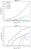 |
Fig. 7. Logarithm of the mEW of the wind emission as a function of NH, plotted for increasing v0 (colour coding, see legend). The soft and hard X-ray bands, corresponding to 0.5–2.5 and 5–15 keV, respectively, are shown with dashed and solid lines. The top and bottom panels correspond to log(ξ0) = 3, 4, respectively. |
5. XRISM Resolve simulations
5.1. Narrow-line Seyfert 1 galaxy spectral energy distribution
In this section, we probe the capability of the Resolve microcalorimeter on board XRISM to constrain the wind emission properties. To do so, we have built a table of WINE spectral templates that are provided as inputs to the xspec fitting software (Arnaud 1996) as table models. We focussed on the following UFO parameter space:
-
log(ξ0)∈[3.0, 5.5], 0.25 step
-
v0 ∈ [0.00, 0.40]c, 0.025 step
-
NH ∈ [0, 2 ⋅ 1024], 1023 step
-
θout ∈ [0, 90deg], 10deg step
-
i ∈ [0, 90deg], 10deg step
and we set all the other properties as in Sect. 3 We note that θout = 0 implies a null volume of the wind cone (see Fig. 1), and therefore corresponds to a null emission spectrum. Since for a given ξ0, NH, the flux of the emitted radiation is proportional to Cf, the strongest emission spectra will be associated with wide-angle winds. To better approximate the attenuation of the emitted radiation in these cases, we set a constant Cv = 1 throughout the parameter space.
Through xspec, we simulated Resolve spectra with the following input model:
 (15)
(15)
where WINEabs and WINEem represent the WINE absorption and emission spectrum, respectively. We note that the gas self-absorption is accounted for during the creation of the emission spectra, and thus it is already implemented in the WINEem component. The powerlaw normalisation was tuned to give a 2–10 flux of 10−11 erg cm−2 s−1, which is representative of the bright targets of the performance verification (PV) phase of XRISM3.
Using this model, we simulated sets of 1000 spectra of 100 ks with several input values for both the ionisation, log(ξ) = 3.5, 4.0,4.5,5.0, and the column density, NH(1023) = 1.0, 2.5, 5.0, 7.5, 10.0, and with v0 = 0.1c. For each observation, we randomly assigned a value for θout, the opening angle of the cone, while for simplicity we fixed i = 0, θin = 0. The spectra were fitted using a two-step approach:
-
First, we fitted the spectrum only with an absorption component (WINEabs ⋅ powerlaw), accurately scanning the parameter space by computing the error and the contour plots associated with each free parameter; that is, log(ξ0),NH, v0.
-
Once a best-fit model was obtained, we included an emission component for which the values of log(ξ0),NH, v0 were tied to those of the absorption component (since emission and absorption are generated by the same medium), and with θout free to vary. Then, we fitted, leaving all the parameters free to vary, and we scanned the parameter space as above.
We used up-to-date response and background files for point source observations for a closed gate valve configuration, available through the XRISM mission website4. Simulated spectra were binned to a minimum of 50 counts per bin and χ2 statistics was adopted. The energy range between 2.0 and 10.0 keV was considered. We verified that the results are the same if a binning with a fixed energy width of 10 eV and C-statistic (Cash 1976) are adopted.
Figure 8 shows the distributions of the 1000 best-fit solutions for an input of log(ξ) = 4. For simplicity, we report only the results for inputs of NH = 1023, 5 ⋅ 1023, 1024 (left, centre, and right columns, respectively). The top, centre, and bottom panels report the best-fit values of NH, ξ, v0, respectively. Hatched and filled histograms represent the distributions before and after the inclusion of the emission component in the fitting model. The last panel shows the best-fit values for θout as a function of their input values. The diagonal black line shows a 1:1 correspondence. Increasing the input for NH (left to right) leads to narrower best-fit distributions, since the wind opacity is higher, and thus tighter constraints can be achieved. The values before and after the inclusion of the emission component basically overlap for NH = 1023, suggesting that the emission component is subdominant in these fits. This is confirmed by the distribution of the values of θout, which is spread over a broad range of the parameter space. We note that the clustering of the output values in steps of 10 deg is simply due to the resolution of the table model. The impact of the emission component grows with an increase in the input NH, as is demonstrated by the increasing distance between the hatched and filled histograms and the tighter correspondence between input and output θout. To provide a more quantitative evaluation of the ability to recover the input parameters, we computed the average Δ as
 (16)
(16)
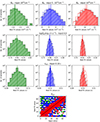 |
Fig. 8. Distribution of the best-fit values of 1000 XRISM Resolve simulations, using as input values log(ξ) = 4.0, v0 = 0.10c and three different NH = 1023, 5 ⋅ 1023, 1024 (left, centre, and right column, respectively). The top, centre, and bottom rows report the best-fit values for NH, log(ξ),v0, respectively. Hatched and filled histograms correspond to the distributions before and after the inclusion of the emission component, respectively. Dashed and solid lines are the median values of the two distributions. Finally, the last panel reports the best-fit values of θout as a function of the input ones. |
that is, the ratio between the best-fit and the input values,  respectively, re-scaled to 0. Figure 9 shows Δ for input log(ξ) = 3.5, 4.0, 4.5, 5.0 as a function of the input NH. The spread corresponds to the standard deviation of the distributions of the best-fit values. For plotting purposes, we only report the values after the inclusion of the emission component. As was expected, Δ is smaller for increasing NH and decreasing ξ; in other words, when the opacity of the wind increases, and thus the fitting results are more constrained. Since we are mainly interested in the characterisation of wide-angle outflows, which are the ones most likely to produce P-Cygni profiles, in the computation of Δ for θout we include only the simulations with input θout ≥ 45deg (≈50% of the total; see Appendix C for the computations with the full dataset).
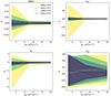 |
Fig. 9. Ratio, Δ (re-scaled to 0; see Eq. 16), between input and best-fit values for XRISM Resolve simulations, as a function of the input, NH. The shaded areas show the corresponding standard deviation. The colour coding corresponds to the different input log(ξ0) (see legend). From left to right and top to bottom, the different panels correspond to the best-fit distributions of log(ξ),v0, NH, θout, respectively. For ease of visualisation, we only report the results after the inclusion of the emission component. Note that, in the last panel, only those simulations with inputs of θout > 45deg are included. |
To give an idea of the capabilities of Resolve with the gate valve open, Fig. 10 shows a simulated 100 ks Resolve spectrum with input parameters of log(ξ) = 4, v0 = 0.10c, NH = 5 ⋅ 1023, θout = 72deg (blue points), together with the fitted model (red line), with best-fit values of  .
.
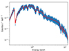 |
Fig. 10. Simulated 100ks XRISMResolve spectrum (blue points) for a wind with log(ξ) = 4, v0 = 0.10c, NH = 5 ⋅ 1023, θout = 72deg and with the gate valve open. The best-fit model is indicated as a red line. The spectrum has been re-binned for plotting purposes. |
5.2. Powerlaw spectral energy distribution
In this section, we adopt a powerlaw function as the input SED and run new simulations to assess its impact on the simulated spectra. We do so to better compare our results with several X-ray observations reported in the literature, in which UFOs have been analysed through photoionisation models assuming such an SED (see e.g. Tombesi et al. 2010; Gofford et al. 2015; Reeves et al. 2023).
We set as reference values a 2–10 keV luminosity of L2 − 10 = 1043 erg s−1 and a black hole mass of MBH = 107 M⊙, implying a value of  for an X-ray bolometric correction of ≈30 (Lusso et al. 2012), a typical value for the bulk of the AGN population in the local Universe (z ≲ 0.1, see e.g. Véron-Cetty & Véron 2006). We set a powerlaw spectral photon index of Γ = 1.8, again to be representative of the local population (see e.g. Piconcelli et al. 2005; Tombesi et al. 2011 and references therein). As above, we assumed an initial radius of r0 = 50rG and a flat density profile (α = 0). The parameter space and the fitting strategy were as above.
We compared this SED and the NLSy1 one in the top panel of Fig. 11, in units of photons s−1 keV−1. Their relative ratio was set as to give the same Lion. The vertical black line corresponds to 13.6 eV; that is, the lower bound of Lion. As was expected, for a given Lion, the NLSy1 SED shows more photons below 0.3 keV. For given ξ, this leads to a higher ionised gas for the powerlaw SED, as can be seen in the second panel, in which we compare the distributions of the iron ionic fractional abundances for ξ = 103, NH = 5 ⋅ 1023, v0 = 0.1c using the two SEDs. While with the NLSy1 SED the most abundant ion is Fe XVII, with the powerlaw SED it is Fe XXVI, and 20% of iron is totally ionised (Fe XXVII). This can also be seen in the spectra of Fig. 11, shown for both cases. We refer to Nicastro et al. (1999a) for a further discussion of the difference between the NLSy1-like and powerlaw SEDs for the gas ionisation.
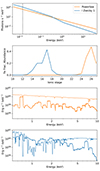 |
Fig. 11. Impact of the SED on the photoionised gas. First panel: Comparison between the powerlaw SED (orange) and the NLSy1 one (blue), in units of photons, s−1 keV−1 (arbitrary normalisation). Second panel: Iron ionic fractional distribution for log(ξ) = 3, NH = 5 ⋅ 1023, v0 = 0.1c and the two different SEDs (colour coding as above). Third and fourth panels: Absorption and emission spectra (thin and thick lines, respectively; units of Erg s−1 keV−1) assuming the powerlaw and the NLSy1 SED, respectively, and the same log(ξ),NH, v0 as in the second panel. |
We simulated sets of 1000 observations with Resolve, following the same procedure as above. Unsurprisingly, we found that the gas emission is totally unconstrained for log(ξ)≥4, the emission being much weaker.
6. Athena X-IFU simulations
To assess the capabilities of the planned X-IFU microcalorimeter on board the Athena satellite, we repeated the same procedure as in Sect. 5.1 using the updated response matrices following the 2023 mission reformulation5. We used the same input model and fitting strategy as in Sect. 5.1. Again, we verified that adopting a 5 eV energy binning and the C-statistic does not change the results. As is shown in Fig. D.1, thanks to its higher effective area and resolution, X-IFU will be able to constrain log(ξ0),vout, NH with uncertainties smaller by a factor of 2, 20, and 5, respectively, and θout with half the uncertainty for input log(ξ0)≤4.0.
Figure 12 shows a simulated spectrum with input log(ξ) = 4, NH = 1023, v0 = 0.10, and the best fit obtained by replacing the NLSy1-SED wind components with those assuming the powerlaw SED. As is shown in Fig. 13 (see also Nicastro et al. 1999a), the different incident SEDs lead to different ionic populations as a function of log(ξ). As a result, the best-fit model is unable to correctly reproduce the Fe L-shell features at E ≈ 1 keV, which are due to a mixture of different ions. Thanks to this, X-IFU will be able to discriminate the incident SED through the absorption (and, eventually, emission) features in the soft band.
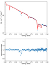 |
Fig. 12. 100 ks simulated X-IFU spectrum for a wind with log(ξ) = 4, NH = 1023, v0 = 0.10c and an NLSy1 incident SED (blue points), best-fitted with a powerlaw-SED WINE table (red line). The bottom panel reports the data for the best-fit model ratio. |
Conversely, it can be seen that the relative abundance of Fe XXV, XXVI, XXVII is similar for the two SEDs, albeit with a shift in the value of log(ξ). Therefore, fitting a spectrum simulated with an NLSy1 SED with a higher log(ξ) = 5, for which these ions are dominant, with a powerlaw SED table yields an acceptable fit with log(ξ) = 3.1. As is shown in Fig. 13 (vertical dashed lines), these values of log(ξ) lead to the same abundance of Fe XXV, XXVI, XXVII with both SEDs.
 |
Fig. 13. Iron ion abundances (computed with XSTAR) as a function of log(ξ) for an optically thin slab and assuming either an NLSy1 (top) or a powerlaw (bottom) incident SED. Dark to light colours correspond to the increasing ionic charge, with the lightest (and rightmost) line being Fe XXVII. Dashed vertical lines in the top and bottom panels correspond, respectively, to the input and best-fit values (see text). |
7. Discussion and conclusions
7.1. Comparison with other wind models
WINE is built on XSTAR, which is a one-dimensional photoionisation code. Such a limitation is addressed by post-processing the gas emissivity and convolving it with three-dimensional line profiles. Therefore, its underlying structure is intrinsically different from three-dimensional Monte-Carlo radiative transfer codes such as DISKWIND (Sim et al. 2008, 2010a,b; Matzeu et al. 2022) and MONACO (Odaka et al. 2011; Hagino et al. 2017) (see Noebauer & Sim 2019 for a review on the models available in the literature). Such codes are able to reproduce with great accuracy the scattering of the radiation by the wind as a function of its geometry and velocity field. However, to cope with the huge computing time required for such simulations, they are based on a number of assumptions concerning the kinematics and the geometry of the wind. Moreover, their photoionisation computation is optimised for a highly ionised gas and focusses mainly on transitions from the K, L, M atomic shells. Due to their fundamental differences, a direct comparison between these models and WINE is not straightforward, but we expect WINE to be more accurate for relatively low Cf and/or low NH; that is, in all those cases in which the reflected spectrum is subdominant with respect to the transmitted one.
The higher degree of freedom in modelling the radial density and velocity profiles in WINE also allows one to better constrain the radial thickness of the wind, Δr (see Eqs. (10)–(13)), which, in turn, can probe r0, n0 (i.e. the launching radius and the wind number density), as was done for the UFO detected in the X-ray spectrum of the AGN PG1448+273 (Laurenti et al. 2021). Together with the covering factor, Cf (which can be derived through WINE once the emission geometry is constrained), such quantities are crucial to accurately compute ̇Mout, ̇Eout. In turn, ̇Mout, ̇Eout are fundamental to probe the impact of the wind on the surrounding environment. By comparing them with the energetics of galaxy-scale outflows, which are typically observed at millimetre to optical wavelengths, it is possible to determine the efficiency of the propagation from the nuclear to the host galaxy scales, and thus to assess the impact on the galaxy life cycle and on the AGN fuelling (so-called ‘AGN feedback’; see e.g. Fiore et al. 2017; Cicone et al. 2018; Marasco et al. 2020; Tozzi et al. 2021).
We finally note that the column density slicing performed in WINE for the ionisation and radiative transfer is the same as for the MHD wind model of Fukumura et al. 2010, 2018, 2022. We aim to extend their analysis of magnetic disc winds through absorption features with the inclusion of the emission spectrum. Moreover, the velocity, density, and thus ionisation profiles predicted for radiatively driven winds, such as in DISKWIND or in Luminari et al. (2021), can be reproduced in WINE, and therefore allow for the comparison of different launching mechanisms within the same code.
7.2. Summary of the results
In this paper, we have outlined the design, initial conditions, and physical picture of the WINE model. We have illustrated some of its main results by simulating the disc winds frequently observed in the X-ray spectra of AGNs. More precisely, we focussed on NLSy1-like galaxies – highly accreting AGNs – where most of the UFOs for which both emission and absorption lines have been detected so far are. Their combination gives rise to the so-called P-Cygni profiles, which are valuable spectroscopic signatures for investigating some of the most elusive wind properties (first of all, the covering factor, Cf) and shedding light on the wind launching, which is hard to constrain by relying on absorption spectroscopy alone. Our main results are the following:
-
The gas opacity, kinematics, and geometry all play a pivotal role in shaping the emission spectrum. The gas opacity depends on the ionisation and on the total (hydrogen-equivalent) column density, which together dictate the ionic column giving rise to the different atomic transitions. Kinematics – that is, the outflow and turbulent velocities, and the geometry – regulate the broadening of the emission profiles via special relativistic Doppler effects. All of these properties must be accounted for to correctly model the emission profiles and, in turn, to derive meaningful physical constraints on the outflowing gas.
-
The incident SED has a strong impact on the gas ionisation. For a given ξ, the gas is much more ionised in the case of a powerlaw SED than in the case of a softer NLSy1- like SED. The gas opacity, and thus the strength of the wind absorption and emission features, are considerably reduced, as is shown in Fig. 11. This may be one of the reason why P-Cygni profiles are more frequently detected in NLSy1-like sources. A similar trend has been observed for UV winds as well. Specifically, the velocity of winds traced by both blueshifted CIV emission and broad, blueshifted CIV absorption correlates with the steepness of the ionising spectrum, usually parametrised through the αOX ratio6 (Nardini et al. 2019; Rankine et al. 2020; Vietri et al. 2020, 2022; Saccheo et al. 2023).
-
We assessed the power of the Resolve microcalorimeter on board XRISM in constraining the UFO parameters – including the emission – of a source with an X-ray flux typical of the targets of the science PV phase (F2 − 10 keV = 10−11 erg cm−2 s−1, see Sect. 5 for details). Assuming an input of vout = 0.1c, we find that, as is shown in Fig. 9, Resolve will be able to constrain log(ξ0),vout with < 5% accuracy and NH with < 40% accuracy for a wind with an input of log(ξ0)≤4.0. For a wind with inputs of log(ξ0)≥4.5 and NH ≥ 5 ⋅ 1023, the accuracy of the best-fit values is within 6% for log(ξ0),vout and 40% for NH. The opening angle of the emitting region, θout, can be determined within a ≈60% accuracy, provided that the input θout is ≥45deg. When considering any input θout, the accuracy reduces to a factor of 2.5 for an input of log(ξ0)≤4.0, NH ≥ 5 ⋅ 1023 (see Appendix C for further details). Figure 14 reports, as a function of input NH, the fraction of simulations in which the absorption and the emission components (left and right panels, respectively) are detected with a significance higher than 2, 3, or 4 σ. For the absorption, the significance was computed as the difference between the best-fit χ2 obtained by fitting the simulated data with a simple powerlaw continuum and with a powerlaw modified by the WINE absorption (WINEabs ⋅ powerlaw). For the emission, the significance was estimated from the difference between the previous absorption-only model and the full model including the wind emission (WINEabs ⋅ powerlaw + WINEem). While the absorption is detected with ≥4σ significance for any input ξ0 and NH ≥ 2.5 ⋅ 1023, the significance of the emission strongly depends on the wind opacity (i.e. it increases for increasing NH and decreasing ξ0). The constraining power is the same for different velocities, provided that the observed opacity is the same; in other words, provided that the intrinsic NH is increased(decreased) for increasing(decreasing) velocity, to compensate for the special relativistic reduction of the opacity according to Eq. (14). The same trend also holds for the X-IFU simulations discussed below.
-
Thanks to its higher effective area and resolution, the X-IFU microcalorimeter on board Athena will allow one to constrain the wind properties with significantly higher accuracy. The absorption is significantly detected in 100% of the simulations, for every input log(ξ0) and NH. As is shown in Fig. 15, the emission is detected with much higher significance than with XRISMResolve (see Fig. 14). For input log(ξ0) = 3.5, 4.0 and NH ≥ 5 ⋅ 1023 cm−2, in > 75% of the simulations the emission is detected at 4σ significance, while for input log(ξ0) = 4.5, NH ≥ 5 ⋅ 1023 cm−2, 50% of the simulations are above the 3σ threshold. Moreover, the Fe L-shell features around 1 keV, which are due to a mixture of different ions, will also allow one to discriminate between a soft and a steep incident ionising SED. While this is not currently possible with Resolve on board XRISM, since the gate valve limits the sensitivity to E ≳ 2 keV, most of its targets will likely be already known, allowing one to reconstruct their SED through data from other observatories.
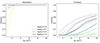 |
Fig. 14. Fraction of the XRISM Resolve simulations in which the WINE absorption (left) and emission (right) components are detected above a given statistical significance, as a function of the input NH. Dotted, dashed, and solid lines correspond to 2, 3, and 4 σ, respectively. |
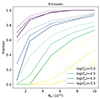 |
Fig. 15. Fraction of the Athena X-IFU simulations in which the WINE emission is detected above a given statistical significance, as a function of the input NH. Dotted, dashed, and solid lines correspond to 2, 3, and 4 σ, respectively. |
7.3. Future upgrades
We plan three main areas of improvement for WINE. First, the computing time needed to build large table models (currently of the order of tens of days for a 50 CPU server) can be dramatically reduced by adopting neural network emulators, such as that presented in Matzeu et al. (2022). Then, we shall increase the modularity of WINE by giving the user the possibility to compute the ionisation balance and radiative transfer with other publicly available codes, such as Cloudy (Ferland et al. 2017). This will allow one to test the impact of the assumptions, limitations, and atomic databases of the different codes on the resulting spectra and to take advantage of the most recent updates of the different codes.
Finally, we aim to implement in WINE an updated version of the Time Evolving PhotoIonisation Device (TEPID; Luminari et al. 2023b), which will be able to model both the time-variable gas absorption and emission spectra, thanks to the inclusion of a detailed electron level population treatment. TEPID will allow one to extend wind modelling beyond the assumption of the photoionisation equilibrium limit. Indeed, time-evolving ionisation is particularly relevant in AGNs, where the ionising luminosity is observed to vary dramatically. The gas equilibration timescale (i.e. the typical time needed by the gas to adjust to luminosity variations) is inversely proportional to its number density, n (Nicastro et al. 1999b), and, for the typical values of X-ray disc winds (especially for WAs), it can be longer than the luminosity variation timescale, leading to a non-equilibrium ionisation dynamic (Rogantini et al. 2022; Sadaula et al. 2023; Luminari et al. 2023b; Gu et al. 2023).
We also note that the perturbation-free assumption in WINE can be relaxed in two main ways. First, it is possible to modify the density and velocity profiles, Eqs. (3), (4), introducing a stochastic fluctuation pattern at perturbation length scales on top of the ‘ideal’ powerlaw trend. Secondly, the synthetic spectra of a multi-phase wind can be represented through the superposition of the absorption or emission features due to the different outflow phases. We shall also consider introducing further degrees of freedom in WINE to account for the wind anisotropy; for example, through the density contrast, δρ/⟨ρ⟩.
7.4. Public release of WINE table models
We make publicly available the WINE table models presented in Sect. 5 at https://baltig.infn.it/ionisation/wine. They can be implemented within the most popular fitting tools, such as xspec, sherpa (Freeman et al. 2001), and spex (Kaastra et al. 1996). The two tables, one with the soft, NLSy1-like SED and one with the powerlaw SEDs, cover a parameter range suited for X-ray disc winds in AGNs, as well as in compact accreting sources, such as X-ray binaries (Fukumura et al. 2017; Tominaga et al. 2023) and ultra-luminous X-ray sources (Pinto et al. 2016; Kosec et al. 2021).
We note that the above codes account, to different extents, for the covering factor of the gas and the presence of velocity gradients. However, such properties only affect the ionisation balance and the radiative transfer but do not affect the profile of the spectral lines.
We find that K = 104 allows one to optimally sample the slab volume, while still being computationally efficient.
The list can be found at: https://xrism.isas.jaxa.jp/research/proposer/approved/pv/index.html
Resolve files can be found at https://xrism.isas.jaxa.jp/research/proposer/obsplan/response/index.html
X-IFU files are available at https://x-ifu.irap.omp.eu/resources/for-the-community
The αOX is defined as the slope connecting the monochromatic luminosities at 2500 Angstrom and 2 keV.
Acknowledgments
AL thanks Massimo Cappi for useful discussions. All the authors thank the IT office from the Roma2 INFN section, particularly Federico Zani, and the rmlab infrastructure for providing computing power for the WINE simulations and for assisting in the creation of the website. We also thank Diego Paris, Elena De Rossi and Federico Fiordoliva from the Astronmical Observatory of Rome (INAF) for computational support and Giustina Vietri for discussions on UV outflows. AL, EP, FN acknowledge support from the HORIZON-2020 grant “Integrated Activities for the High Energy Astrophysics Domain” (AHEAD-2020), G.A. 871158). EP, FT acknowledges funding from the European Union – Next Generation EU, PRIN/MUR 2022 2022K9N5B4. We used ASTROPY (http://www.astropy.org), a community-developed core PYTHON package for Astronomy (Astropy Collaboration 2018), NUMPY (Harris et al. 2020) and MATPLOTLIB (Hunter 2007).
References
- Arav, N., de Kool, M., Korista, K. T., et al. 2001, ApJ, 561, 118 [NASA ADS] [CrossRef] [Google Scholar]
- Arnaud, K. A. 1996, ASP Conf. Ser., 101, 17 [Google Scholar]
- Astropy Collaboration (Price-Whelan, A. M., et al.) 2018, AJ, 156, 123 [Google Scholar]
- Barret, D., & Cappi, M. 2019, A&A, 628, A5 [NASA ADS] [CrossRef] [EDP Sciences] [Google Scholar]
- Barret, D., Albouys, V., den Herder, J.-W., et al. 2023, Exp. Astron., 55, 373 [NASA ADS] [CrossRef] [Google Scholar]
- Bischetti, M., Feruglio, C., D’Odorico, V., et al. 2022, Nature, 605, 244 [NASA ADS] [CrossRef] [Google Scholar]
- Blustin, A. J., Page, M. J., Fuerst, S. V., Branduardi-Raymont, G., & Ashton, C. E. 2005, A&A, 431, 111 [CrossRef] [EDP Sciences] [Google Scholar]
- Braito, V., Reeves, J. N., Matzeu, G. A., et al. 2018, MNRAS, 479, 3592 [Google Scholar]
- Bruni, G., Piconcelli, E., Misawa, T., et al. 2019, A&A, 630, A111 [NASA ADS] [CrossRef] [EDP Sciences] [Google Scholar]
- Cappi, M., Tombesi, F., Bianchi, S., et al. 2009, A&A, 504, 401 [NASA ADS] [CrossRef] [EDP Sciences] [Google Scholar]
- Cash, W. 1976, A&A, 52, 307 [NASA ADS] [Google Scholar]
- Castor, J. I., & Lamers, H. J. G. L. M. 1979, ApJS, 39, 481 [NASA ADS] [CrossRef] [Google Scholar]
- Chartas, G., Cappi, M., Vignali, C., et al. 2021, ApJ, 920, 24 [NASA ADS] [CrossRef] [Google Scholar]
- Cicone, C., Brusa, M., Ramos Almeida, C., et al. 2018, Nat. Astron., 2, 176 [Google Scholar]
- Crenshaw, D. M., & Kraemer, S. B. 2012, ApJ, 753, 75 [NASA ADS] [CrossRef] [Google Scholar]
- Cui, C., & Yuan, F. 2020, ApJ, 890, 81 [NASA ADS] [CrossRef] [Google Scholar]
- Dannen, R. C., Proga, D., Waters, T., & Dyda, S. 2020, ApJ, 893, L34 [Google Scholar]
- Elvis, M. 2000, ApJ, 545, 63 [NASA ADS] [CrossRef] [Google Scholar]
- Faucher-Giguère, C.-A., & Quataert, E. 2012, MNRAS, 425, 605 [Google Scholar]
- Ferland, G. J., Chatzikos, M., Guzmán, F., et al. 2017, Rev. Mex. Astron. Astrofis., 53, 385 [NASA ADS] [Google Scholar]
- Feruglio, C., Fiore, F., Carniani, S., et al. 2015, A&A, 583, A99 [NASA ADS] [CrossRef] [EDP Sciences] [Google Scholar]
- Fiore, F., Feruglio, C., Shankar, F., et al. 2017, A&A, 601, A143 [NASA ADS] [CrossRef] [EDP Sciences] [Google Scholar]
- Fiore, F., Gaspari, M., Luminari, A., Tozzi, P., & de Arcangelis, L. 2024, A&A, 686, A36 [NASA ADS] [CrossRef] [EDP Sciences] [Google Scholar]
- Freeman, P., Doe, S., & Siemiginowska, A. 2001, SPIE Conf. Ser., 4477, 76 [NASA ADS] [Google Scholar]
- Fukumura, K., Kazanas, D., Contopoulos, I., & Behar, E. 2010, ApJ, 715, 636 [NASA ADS] [CrossRef] [Google Scholar]
- Fukumura, K., Tombesi, F., Kazanas, D., et al. 2014, ApJ, 780, 120 [Google Scholar]
- Fukumura, K., Kazanas, D., Shrader, C., et al. 2017, Nat. Astron., 1, 0062 [NASA ADS] [CrossRef] [Google Scholar]
- Fukumura, K., Kazanas, D., Shrader, C., et al. 2018, ApJ, 864, L27 [NASA ADS] [CrossRef] [Google Scholar]
- Fukumura, K., Dadina, M., Matzeu, G., et al. 2022, ApJ, 940, 6 [NASA ADS] [CrossRef] [Google Scholar]
- Gofford, J., Reeves, J. N., Tombesi, F., et al. 2013, MNRAS, 430, 60 [Google Scholar]
- Gofford, J., Reeves, J. N., McLaughlin, D. E., et al. 2015, MNRAS, 451, 4169 [Google Scholar]
- Gu, L., Kaastra, J., Rogantini, D., et al. 2023, A&A, 679, A43 [NASA ADS] [CrossRef] [EDP Sciences] [Google Scholar]
- Hagino, K., Odaka, H., Done, C., et al. 2015, MNRAS, 446, 663 [NASA ADS] [CrossRef] [Google Scholar]
- Hagino, K., Odaka, H., Done, C., et al. 2016, MNRAS, 461, 3954 [Google Scholar]
- Hagino, K., Done, C., Odaka, H., Watanabe, S., & Takahashi, T. 2017, MNRAS, 468, 1442 [NASA ADS] [CrossRef] [Google Scholar]
- Harris, C. R., Millman, K. J., van der Walt, S. J., et al. 2020, Nature, 585, 357 [NASA ADS] [CrossRef] [Google Scholar]
- Higginbottom, N., Proga, D., Knigge, C., et al. 2014, ApJ, 789, 19 [NASA ADS] [CrossRef] [Google Scholar]
- Hunter, J. D. 2007, Comput. Sci. Eng., 9, 90 [NASA ADS] [CrossRef] [Google Scholar]
- Jansen, F., Lumb, D., Altieri, B., et al. 2001, A&A, 365, L1 [NASA ADS] [CrossRef] [EDP Sciences] [Google Scholar]
- Kaastra, J. S., Mewe, R., & Nieuwenhuijzen, H. 1996, UV and X-ray Spectroscopy of Astrophysical and Laboratory Plasmas, 411 [Google Scholar]
- Kaastra, J. S., Kriss, G. A., Cappi, M., et al. 2014, Science, 345, 64 [Google Scholar]
- Kallman, T. R., Palmeri, P., Bautista, M. A., Mendoza, C., & Krolik, J. H. 2004, ApJS, 155, 675 [Google Scholar]
- Kallman, T., Bautista, M., Deprince, J., et al. 2021, ApJ, 908, 94 [NASA ADS] [CrossRef] [Google Scholar]
- King, A., & Pounds, K. 2015, ARA&A, 53, 115 [NASA ADS] [CrossRef] [Google Scholar]
- Kollatschny, W., Reichstein, A., & Zetzl, M. 2012, A&A, 548, A37 [NASA ADS] [CrossRef] [EDP Sciences] [Google Scholar]
- Komossa, S. 2008, Rev. Mex. Astron. Astrofis. Conf. Ser., 32, 86 [Google Scholar]
- Kosec, P., Zoghbi, A., Walton, D. J., et al. 2020, MNRAS, 495, 4769 [CrossRef] [Google Scholar]
- Kosec, P., Pinto, C., Reynolds, C. S., et al. 2021, MNRAS, 508, 3569 [NASA ADS] [CrossRef] [Google Scholar]
- Krongold, Y., Nicastro, F., Elvis, M., et al. 2007, ApJ, 659, 1022 [NASA ADS] [CrossRef] [Google Scholar]
- Laha, S., Reynolds, C. S., Reeves, J., et al. 2021, Nat. Astron., 5, 13 [NASA ADS] [CrossRef] [Google Scholar]
- Laurenti, M., Luminari, A., Tombesi, F., et al. 2021, A&A, 645, A118 [NASA ADS] [CrossRef] [EDP Sciences] [Google Scholar]
- Luminari, A., Piconcelli, E., Tombesi, F., et al. 2018, A&A, 619, A149 [NASA ADS] [CrossRef] [EDP Sciences] [Google Scholar]
- Luminari, A., Tombesi, F., Piconcelli, E., et al. 2020, A&A, 633, A55 [NASA ADS] [CrossRef] [EDP Sciences] [Google Scholar]
- Luminari, A., Nicastro, F., Elvis, M., et al. 2021, A&A, 646, A111 [NASA ADS] [CrossRef] [EDP Sciences] [Google Scholar]
- Luminari, A., Marinucci, A., Bianchi, S., et al. 2023a, ApJ, 950, 160 [NASA ADS] [CrossRef] [Google Scholar]
- Luminari, A., Nicastro, F., Krongold, Y., Piro, L., & Thakur, A. L. 2023b, A&A, 679, A141 [NASA ADS] [CrossRef] [EDP Sciences] [Google Scholar]
- Lusso, E., Comastri, A., Simmons, B. D., et al. 2012, MNRAS, 425, 623 [Google Scholar]
- Maksym, W. P., Elvis, M., Fabbiano, G., et al. 2023, ApJ, 951, 146 [NASA ADS] [CrossRef] [Google Scholar]
- Mao, J., Kriss, G. A., Landt, H., et al. 2022, ApJ, 940, 41 [NASA ADS] [CrossRef] [Google Scholar]
- Marasco, A., Cresci, G., Nardini, E., et al. 2020, A&A, 644, A15 [EDP Sciences] [Google Scholar]
- Marzi, M., Tombesi, F., Luminari, A., Fukumura, K., & Kazanas, D. 2023, A&A, 670, A122 [NASA ADS] [CrossRef] [EDP Sciences] [Google Scholar]
- Mason, K. O., Breeveld, A., Much, R., et al. 2001, A&A, 365, L36 [NASA ADS] [CrossRef] [EDP Sciences] [Google Scholar]
- Matthews, J. H. 2016, Ph.D. Thesis, University of Southampton, UK [Google Scholar]
- Matthews, J. H., Knigge, C., Long, K. S., et al. 2016, MNRAS, 458, 293 [NASA ADS] [CrossRef] [Google Scholar]
- Matthews, J. H., Knigge, C., Higginbottom, N., et al. 2020, MNRAS, 492, 5540 [NASA ADS] [CrossRef] [Google Scholar]
- Matzeu, G. A., Braito, V., Reeves, J. N., et al. 2019, MNRAS, 483, 2836 [Google Scholar]
- Matzeu, G. A., Lieu, M., Costa, M. T., et al. 2022, MNRAS, 515, 6172 [NASA ADS] [CrossRef] [Google Scholar]
- Matzeu, G. A., Brusa, M., Lanzuisi, G., et al. 2023, A&A, 670, A182 [Google Scholar]
- Menci, N., Fiore, F., Feruglio, C., et al. 2019, ApJ, 877, 74 [NASA ADS] [CrossRef] [Google Scholar]
- Menci, N., Fiore, F., Shankar, F., Zanisi, L., & Feruglio, C. 2023, A&A, 674, A181 [NASA ADS] [CrossRef] [EDP Sciences] [Google Scholar]
- Middei, R., Nardini, E., Matzeu, G. A., et al. 2023, A&A, 680, A50 [NASA ADS] [CrossRef] [EDP Sciences] [Google Scholar]
- Mingozzi, M., Cresci, G., Venturi, G., et al. 2019, A&A, 622, A146 [NASA ADS] [CrossRef] [EDP Sciences] [Google Scholar]
- Moos, H. W., Cash, W. C., Cowie, L. L., et al. 2000, ApJ, 538, L1 [NASA ADS] [CrossRef] [Google Scholar]
- Murray, N., Chiang, J., Grossman, S. A., & Voit, G. M. 1995, ApJ, 451, 498 [NASA ADS] [CrossRef] [Google Scholar]
- Nardini, E., Reeves, J. N., Gofford, J., et al. 2015, Science, 347, 860 [Google Scholar]
- Nardini, E., Lusso, E., Risaliti, G., et al. 2019, A&A, 632, A109 [NASA ADS] [CrossRef] [EDP Sciences] [Google Scholar]
- Nicastro, F., Fiore, F., & Matt, G. 1999a, ApJ, 517, 108 [NASA ADS] [CrossRef] [Google Scholar]
- Nicastro, F., Fiore, F., Perola, G. C., & Elvis, M. 1999b, ApJ, 512, 184 [NASA ADS] [CrossRef] [Google Scholar]
- Noebauer, U. M., & Sim, S. A. 2019, Liv. Rev. Comput. Astrophys., 5, 1 [CrossRef] [Google Scholar]
- Odaka, H., Aharonian, F., Watanabe, S., et al. 2011, ApJ, 740, 103 [NASA ADS] [CrossRef] [Google Scholar]
- Ohsuga, K., Mineshige, S., Mori, M., & Kato, Y. 2009, PASJ, 61, L7 [NASA ADS] [Google Scholar]
- Parker, M. L., Pinto, C., Fabian, A. C., et al. 2017, Nature, 543, 83 [Google Scholar]
- Parker, M. L., Matzeu, G. A., Matthews, J. H., et al. 2022, MNRAS, 513, 551 [NASA ADS] [CrossRef] [Google Scholar]
- Piconcelli, E., Jimenez-Bailón, E., Guainazzi, M., et al. 2005, A&A, 432, 15 [NASA ADS] [CrossRef] [EDP Sciences] [Google Scholar]
- Pinto, C., Middleton, M. J., & Fabian, A. C. 2016, Nature, 533, 64 [Google Scholar]
- Pounds, K. A., Reeves, J. N., King, A. R., et al. 2003, MNRAS, 345, 705 [Google Scholar]
- Proga, D., & Kallman, T. R. 2004, ApJ, 616, 688 [Google Scholar]
- Proga, D., Stone, J. M., & Kallman, T. R. 2000, ApJ, 543, 686 [Google Scholar]
- Rakshit, S., Stalin, C. S., Chand, H., & Zhang, X.-G. 2017, ApJS, 229, 39 [Google Scholar]
- Rankine, A. L., Hewett, P. C., Banerji, M., & Richards, G. T. 2020, MNRAS, 492, 4553 [CrossRef] [Google Scholar]
- Reeves, J. N., & Braito, V. 2019, ApJ, 884, 80 [NASA ADS] [CrossRef] [Google Scholar]
- Reeves, J. N., Braito, V., Porquet, D., et al. 2023, ApJ, 952, 52 [NASA ADS] [CrossRef] [Google Scholar]
- Rogantini, D., Mehdipour, M., Kaastra, J., et al. 2022, ApJ, 940, 122 [NASA ADS] [CrossRef] [Google Scholar]
- Rupke, D. S. N., & Veilleux, S. 2013, ApJ, 768, 75 [Google Scholar]
- Saccheo, I., Bongiorno, A., Piconcelli, E., et al. 2023, A&A, 671, A34 [NASA ADS] [CrossRef] [EDP Sciences] [Google Scholar]
- Sadaula, D. R., Bautista, M. A., García, J. A., & Kallman, T. R. 2023, ApJ, 946, 93 [NASA ADS] [CrossRef] [Google Scholar]
- Saez, C., & Chartas, G. 2011, ApJ, 737, 91 [NASA ADS] [CrossRef] [Google Scholar]
- Sahnow, D. J., Moos, H. W., Ake, T. B., et al. 2000, ApJ, 538, L7 [NASA ADS] [CrossRef] [Google Scholar]
- Schurch, N. J., & Done, C. 2007, MNRAS, 381, 1413 [NASA ADS] [CrossRef] [Google Scholar]
- Sim, S. A., Long, K. S., Miller, L., & Turner, T. J. 2008, MNRAS, 388, 611 [CrossRef] [Google Scholar]
- Sim, S. A., Miller, L., Long, K. S., Turner, T. J., & Reeves, J. N. 2010a, MNRAS, 404, 1369 [NASA ADS] [Google Scholar]
- Sim, S. A., Proga, D., Miller, L., Long, K. S., & Turner, T. J. 2010b, MNRAS, 408, 1396 [NASA ADS] [CrossRef] [Google Scholar]
- Smith, R. N., Tombesi, F., Veilleux, S., Lohfink, A. M., & Luminari, A. 2019, ApJ, 887, 69 [NASA ADS] [CrossRef] [Google Scholar]
- Strüder, L., Briel, U., Dennerl, K., et al. 2001, A&A, 365, L18 [Google Scholar]
- Tarchi, A., Castangia, P., Columbano, A., Panessa, F., & Braatz, J. A. 2011, A&A, 532, A125 [NASA ADS] [CrossRef] [EDP Sciences] [Google Scholar]
- Tarter, C. B., Tucker, W. H., & Salpeter, E. E. 1969, ApJ, 156, 943 [Google Scholar]
- Tashiro, M., Maejima, H., Toda, K., et al. 2020, SPIE Conf. Ser., 11444, 1144422 [Google Scholar]
- Tombesi, F., Cappi, M., Reeves, J. N., et al. 2010, A&A, 521, A57 [NASA ADS] [CrossRef] [EDP Sciences] [Google Scholar]
- Tombesi, F., Cappi, M., Reeves, J. N., et al. 2011, ApJ, 742, 44 [Google Scholar]
- Tombesi, F., Cappi, M., Reeves, J. N., & Braito, V. 2012, MNRAS, 422, L1 [Google Scholar]
- Tominaga, M., Tsujimoto, M., Ebisawa, K., Enoto, T., & Hayasaki, K. 2023, ApJ, 958, 52 [NASA ADS] [CrossRef] [Google Scholar]
- Torrey, P., Hopkins, P. F., Faucher-Giguère, C.-A., et al. 2020, MNRAS, 497, 5292 [NASA ADS] [CrossRef] [Google Scholar]
- Tozzi, G., Cresci, G., Marasco, A., et al. 2021, A&A, 648, A99 [NASA ADS] [CrossRef] [EDP Sciences] [Google Scholar]
- Turner, M. J. L., Abbey, A., Arnaud, M., et al. 2001, A&A, 365, L27 [CrossRef] [EDP Sciences] [Google Scholar]
- Venturi, G., Nardini, E., Marconi, A., et al. 2018, A&A, 619, A74 [NASA ADS] [CrossRef] [EDP Sciences] [Google Scholar]
- Véron-Cetty, M. P., & Véron, P. 2006, A&A, 455, 773 [Google Scholar]
- Vietri, G., Mainieri, V., Kakkad, D., et al. 2020, A&A, 644, A175 [NASA ADS] [CrossRef] [EDP Sciences] [Google Scholar]
- Vietri, G., Misawa, T., Piconcelli, E., et al. 2022, A&A, 668, A87 [NASA ADS] [CrossRef] [EDP Sciences] [Google Scholar]
- Waters, T., Proga, D., & Dannen, R. 2021, ApJ, 914, 62 [NASA ADS] [CrossRef] [Google Scholar]
- Waters, T., Proga, D., Dannen, R., & Dyda, S. 2022, ApJ, 931, 134 [NASA ADS] [CrossRef] [Google Scholar]
- Yamamoto, R., & Fukue, J. 2021, MNRAS, 502, 5797 [NASA ADS] [CrossRef] [Google Scholar]
- Yuan, F., Gan, Z., Narayan, R., et al. 2015, ApJ, 804, 101 [NASA ADS] [CrossRef] [Google Scholar]
Appendix A: Perpendicular velocity components
The main effect of an eventual velocity component perpendicular to the LOS, such as that due to Keplerian rotation, will be to increase the angle θ between the total wind velocity and the LOS (which for a pure outward radial motion is = 0) and, thus, to modify the relativistic factors ψ, ψ3 of Eq. 9, regulating respectively the wavelength shift and the beaming in the wind reference frame. To assess the impact of this on the wind interaction with the radiation field, we compared ψ, ψ3 for a pure outward motion (as assumed in WINE) with vout = 0.1, 0.3 c and adding a transverse rotational component corresponding to the Keplerian rotational velocity v  for different launching radii r0, i.e. ψrot, ψrot3.
Figure A.1. top panel, shows vrot as a function of r0. Middle panels report, as a function of r0, θ (left) and ψrot, ψrot3 (right) including vrot and vout = 0.1, 0.3 c. For comparison, ψ, ψ3 are plotted with dashed lines. Within ∼ 10 RS, the inclusion of vrot leads to a strong increase of θ, i.e. the motion is almost perpendicular to the LOS. Consequently, both ψrot, ψrot3 are very small, resulting in spectroscopic signatures with small blueshift and limited interaction between the gas and the radiation field, respectively. For increasing r0, vrot decreases and, accordingly, θ is closer to 0 and ψrot, ψrot3 tend to ψ, ψ3. The bottom panel reports the ratios ψrot/ψ and ψrot3/ψ3. For r0 = 10 RS, ψrot/ψ = 0.93 and ψrot3/ψ3 = 0.85, while for r0 = 100 RS they are both > 0.999. The blueshift and the opacity of the observed absorption features as measured by WINE (and, thus, the derived v and NH) can be corrected by multiplying them by ψrot/ψ and ψrot3/ψ3, provided that the radial location of the wind (or, equivalently, the ratio between outflow and rotational velocity components) can be estimated. Such a-posteriori correction cannot be performed for the emission profiles which, unlike the absorption, are integrated over the outflow solid angle. However, the ratios above provide an overview of the expected variation of the velocity broadening and equivalent width of the profiles, respectively.
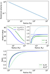 |
Fig. A.1. Impact of a velocity component perpendicular to the LOS. Top: rotational velocity vrot (in units of c) as a function of the disc radius (in units of RS). Middle, both as a function of the radius; left: angle θ between the LOS and the total velocity for vrad = 0.1, 0.3 c (colour coding; see legend); right: relativistic factors ψrot, ψrot3 for the same total velocity (dark and light colours, respectively). For comparison, dashed lines report ψ, ψ3, i.e. the same factors computed neglecting vrot. Bottom: ratio between the relativistic factors: dark ad light colours correspond to ψrot/ψ and ψrot3/ψ3, respectively. Colour coding as above. |
Appendix B: Comparison between WINE and XSTAR
Figure B.1 shows the comparison between the absorption spectra computed with WINE and XSTAR (green and blue lines, respectively) for ξ = 103 and NH = 5 ⋅ 1023, 1024 (top and bottom panel, respectively). As discussed in Sect. 2, WINE spectra are built by dividing the wind column in a series of thin slabs (with a linear thickness of 5 ⋅ 1022 in this example) and computing photoionisation and radiative transfer iteratively, from the innermost to the outermost. Wind emission is computed in post-processing, therefore the emitted radiation does not affect radiative transfer and the resulting absorption spectrum. Conversely, XSTAR spectra are computed giving as input the whole column density and, thus, the emitted radiation is accounted for automatically by the code during the radiative transfer. This leads to slightly smaller opacities in the XSTAR spectra. However, as can be seen in the figure, the differences in terms of fluxes per unit keV are very small, of the order of 10−5 and 10−16 with respect to the incident continuum for NH = 5 ⋅ 1023 and 1024, respectively, showing that the WINE slicing does not lead to dramatic changes in the absorption spectra even for such high wind opacities.
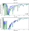 |
Fig. B.1. Comparison between WINE- and XSTAR-generated absorption spectra for log(ξ)3 and NH = 5 ⋅ 1023, 1024 (top and bottom panel, respectively). Blue lines correspond to the XSTAR results, green to the WINE ones. For ease of visualisation, the spectra are divided by the incident continuum. |
Appendix C: XRISM Resolve simulations
Figure C.1 shows the ratio, Δ, between input and best fit values for θout, including all the simulations.
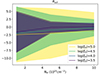 |
Fig. C.1. Ratio Δ and corresponding standard deviations for XRISM Resolve simulations, relative to θout, as a function of input NH and for different input log(ξ0) (see legend). |
Appendix D: Athena X-IFU simulations
Figure D.1 shows the ratio Δ for the Athena X-IFU simulations. For ease of comparison with the XRISM results in Fig. 9, bottom right panel reports only the cases with input θout > 45deg.
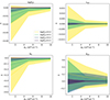 |
Fig. D.1. Ratio Δ and corresponding standard deviations for Athena X-IFU, as a function of input NH and for different input log(ξ0) (see legend). |
All Figures
|
Fig. 1. Geometry of the WINE model. The shaded grey area indicates the wind volume. θin, θout represents the wind inner and outer opening angle with respect to the symmetry axis (vertical dotted line). The LOS has an inclination angle, i, with respect to the axis. The accretion disc is represented with a yellow bar, and the black and blue dots indicate, respectively, the accreting and the luminosity sources, which are assumed to be point-like. Finally, r0, r1 indicate the wind’s initial and final radius, respectively. |
| In the text | |
|
Fig. 2. UV-to-X-ray SED of the NLSy1 I Zwicky 1. |
| In the text | |
|
Fig. 3. Impact of the relativistic effects on the asorption features. Top: Absorption profiles for v0 = 0.00, 0.10, 0.30c (colour coding, see legend) and NH = 1023, log(ξ0) = 4 in the rest-frame spectrum between 6–10 keV. For increasing v0, absorption lines are increasingly blueshifted and show lower EWs, as was expected from special relativity effects. Bottom: Ratio, Ψrel, between intrinsic and observed gas opacity as a function of the gas velocity, v (in units of c). |
| In the text | |
|
Fig. 4. Emission profiles for different wind geometries, assuming log(ξ0) = 3, v0 = 0.10c, NH = 1023. Top row: Wind seen ‘face on’ (i = 0) and θout = 90, 30 deg (left and right panel, respectively). Bottom row: ‘Edge-on’ winds (i = 90 deg) and θout = 90, 30 (left and right panel, respectively). For comparison, the i = 0, θout = 90 deg case is reported with light grey lines in all the panels. |
| In the text | |
|
Fig. 5. WINE spectrum for log(ξ0) = 3, NH = 5 ⋅ 1023 and v0 = 0.0, 0.1 c (top and bottom row, respectively). The left panels show the E = 1–8.5 keV spectrum, while the right panels zoom in above E = 6 keV. Orange(red) lines represent the emission spectrum and pink(purple) the total (absorption + emission) spectrum for Cv = 0(1). The absorption spectrum is shown with dashed black lines. For ease of visualisation, the spectra are divided by the incident continuum. |
| In the text | |
|
Fig. 6. WINE spectrum for log(ξ0) = 4, NH = 5 ⋅ 1023 and v0 = 0.0, 0.1 c (top and bottom panel, respectively). The colour coding is as in Fig. 5. |
| In the text | |
|
Fig. 7. Logarithm of the mEW of the wind emission as a function of NH, plotted for increasing v0 (colour coding, see legend). The soft and hard X-ray bands, corresponding to 0.5–2.5 and 5–15 keV, respectively, are shown with dashed and solid lines. The top and bottom panels correspond to log(ξ0) = 3, 4, respectively. |
| In the text | |
|
Fig. 8. Distribution of the best-fit values of 1000 XRISM Resolve simulations, using as input values log(ξ) = 4.0, v0 = 0.10c and three different NH = 1023, 5 ⋅ 1023, 1024 (left, centre, and right column, respectively). The top, centre, and bottom rows report the best-fit values for NH, log(ξ),v0, respectively. Hatched and filled histograms correspond to the distributions before and after the inclusion of the emission component, respectively. Dashed and solid lines are the median values of the two distributions. Finally, the last panel reports the best-fit values of θout as a function of the input ones. |
| In the text | |
|
Fig. 9. Ratio, Δ (re-scaled to 0; see Eq. 16), between input and best-fit values for XRISM Resolve simulations, as a function of the input, NH. The shaded areas show the corresponding standard deviation. The colour coding corresponds to the different input log(ξ0) (see legend). From left to right and top to bottom, the different panels correspond to the best-fit distributions of log(ξ),v0, NH, θout, respectively. For ease of visualisation, we only report the results after the inclusion of the emission component. Note that, in the last panel, only those simulations with inputs of θout > 45deg are included. |
| In the text | |
|
Fig. 10. Simulated 100ks XRISMResolve spectrum (blue points) for a wind with log(ξ) = 4, v0 = 0.10c, NH = 5 ⋅ 1023, θout = 72deg and with the gate valve open. The best-fit model is indicated as a red line. The spectrum has been re-binned for plotting purposes. |
| In the text | |
|
Fig. 11. Impact of the SED on the photoionised gas. First panel: Comparison between the powerlaw SED (orange) and the NLSy1 one (blue), in units of photons, s−1 keV−1 (arbitrary normalisation). Second panel: Iron ionic fractional distribution for log(ξ) = 3, NH = 5 ⋅ 1023, v0 = 0.1c and the two different SEDs (colour coding as above). Third and fourth panels: Absorption and emission spectra (thin and thick lines, respectively; units of Erg s−1 keV−1) assuming the powerlaw and the NLSy1 SED, respectively, and the same log(ξ),NH, v0 as in the second panel. |
| In the text | |
|
Fig. 12. 100 ks simulated X-IFU spectrum for a wind with log(ξ) = 4, NH = 1023, v0 = 0.10c and an NLSy1 incident SED (blue points), best-fitted with a powerlaw-SED WINE table (red line). The bottom panel reports the data for the best-fit model ratio. |
| In the text | |
|
Fig. 13. Iron ion abundances (computed with XSTAR) as a function of log(ξ) for an optically thin slab and assuming either an NLSy1 (top) or a powerlaw (bottom) incident SED. Dark to light colours correspond to the increasing ionic charge, with the lightest (and rightmost) line being Fe XXVII. Dashed vertical lines in the top and bottom panels correspond, respectively, to the input and best-fit values (see text). |
| In the text | |
|
Fig. 14. Fraction of the XRISM Resolve simulations in which the WINE absorption (left) and emission (right) components are detected above a given statistical significance, as a function of the input NH. Dotted, dashed, and solid lines correspond to 2, 3, and 4 σ, respectively. |
| In the text | |
|
Fig. 15. Fraction of the Athena X-IFU simulations in which the WINE emission is detected above a given statistical significance, as a function of the input NH. Dotted, dashed, and solid lines correspond to 2, 3, and 4 σ, respectively. |
| In the text | |
|
Fig. A.1. Impact of a velocity component perpendicular to the LOS. Top: rotational velocity vrot (in units of c) as a function of the disc radius (in units of RS). Middle, both as a function of the radius; left: angle θ between the LOS and the total velocity for vrad = 0.1, 0.3 c (colour coding; see legend); right: relativistic factors ψrot, ψrot3 for the same total velocity (dark and light colours, respectively). For comparison, dashed lines report ψ, ψ3, i.e. the same factors computed neglecting vrot. Bottom: ratio between the relativistic factors: dark ad light colours correspond to ψrot/ψ and ψrot3/ψ3, respectively. Colour coding as above. |
| In the text | |
|
Fig. B.1. Comparison between WINE- and XSTAR-generated absorption spectra for log(ξ)3 and NH = 5 ⋅ 1023, 1024 (top and bottom panel, respectively). Blue lines correspond to the XSTAR results, green to the WINE ones. For ease of visualisation, the spectra are divided by the incident continuum. |
| In the text | |
|
Fig. C.1. Ratio Δ and corresponding standard deviations for XRISM Resolve simulations, relative to θout, as a function of input NH and for different input log(ξ0) (see legend). |
| In the text | |
|
Fig. D.1. Ratio Δ and corresponding standard deviations for Athena X-IFU, as a function of input NH and for different input log(ξ0) (see legend). |
| In the text | |
Current usage metrics show cumulative count of Article Views (full-text article views including HTML views, PDF and ePub downloads, according to the available data) and Abstracts Views on Vision4Press platform.
Data correspond to usage on the plateform after 2015. The current usage metrics is available 48-96 hours after online publication and is updated daily on week days.
Initial download of the metrics may take a while.