| Issue |
A&A
Volume 691, November 2024
|
|
|---|---|---|
| Article Number | A267 | |
| Number of page(s) | 13 | |
| Section | Planets and planetary systems | |
| DOI | https://doi.org/10.1051/0004-6361/202346361 | |
| Published online | 18 November 2024 | |
Multiple reference star differential imaging with VLT/SPHERE
Influence of the reference frame selection and library★
1
Univ. Grenoble Alpes, CNRS, IPAG,
38000
Grenoble,
France
2
European Southern Observatory,
Alonso de Córdova 3107, Vitacura, Casilla
19001,
Santiago de Chile,
Chile
3
LESIA, Observatoire de Paris, PSL Research University, CNRS, Sorbonne Universités,
UPMC Univ. Paris 06, Univ. Paris Diderot,
Sorbonne Paris Cité,
France
4
Department of Astronomy and Steward Observatory, University of Arizona,
933 N. Cherry Avenue,
Tucson,
AZ
85721-0065,
USA
5
Large Binocular Telescope Observatory, University of Arizona,
933 N. Cherry Avenue,
Tucson,
AZ
85721-0065,
USA
6
Instituto de Astrofísica de Canarias,
Calle Vía Láctea S/N,
38205
La Laguna,
Tenerife,
Spain
7
Instituto Nacional de Astrofésica, Optica y Electrónica,
Luis Enrique Erro 1, Sta. Ma. Tonantzintla,
Puebla,
Mexico
★★ Corresponding author; This email address is being protected from spambots. You need JavaScript enabled to view it.
Received:
9
March
2023
Accepted:
30
August
2024
Abstract
Context. High-contrast imaging observations mostly rely on angular differential imaging, a successful technique for detecting point-sources, such as planets. However, in the vicinity of the star (typically below 300 mas), this technique suffers from signal self-subtraction when there is not enough field rotation. Building large libraries of reference stars from archival data later used to optimally subtract the stellar halo is a powerful technique known as reference star differential imaging (RSDI) that can overcome this limitation.
Aims. We aim at investigating new methods for creating reference libraries composed of multiple stars when applying reference star differential imaging to VLT/SPHERE data. We used for that purpose a data set from the SPHERE High Angular Resolution Debris Disk Survey (SHARDDS), composed of 55 targets observed in broad-band H with the InfraRed Dual-band Imager and Spectrograph (IRDIS) during 2015-2016, with a total of ~20 000 frames. We consider HD 206893, known to host a close-in bound substellar companion HD 206893 B, as a benchmark science target to demonstrate the improved sensitivity provided by this method.
Methods. We created libraries of reference frames based on different image similarity metrics: the cosine distance between descriptors created by a convolutional neural network, the Pearson correlation coefficient, the Structural Similarity Index, the Strehl ratio, and raw contrast criteria. We used principal component analysis (PCA) to subtract the stellar halo and tested various normalization options.
Results. We obtained the best signal-to-noise ratio (S/N) on HD 206893 B by using the Pearson correlation coefficient (PCC) applied to an annulus between 245 and 612 mas to select reference frames. The ten reference libraries with the highest S/N on the substellar companion HD 206893 B were all based on the PCC method, outperforming other similarity metrics. While the Strehl ratio is the environment variable most correlated to the contrast, it is insufficient to select similar images. We also show that having multiple reference stars in the reference library produces better results than using a single well-chosen reference star.
Conclusions. Using the Pearson correlation computed on a specific area of interest to select reference frames is a promising alternative to improve the detectability of faint point-sources when applying reference star differential imaging. In the future, reducing all the data available in the SPHERE archive using this technique might offer interesting results in the search for previously undetected planets.
Key words: instrumentation: high angular resolution / methods: data analysis / methods: statistical / techniques: image processing
Based on observations collected at the European Southern Observatory under ESO programmes 096.C-0388(A) and 097.C-0394(A).
© The Authors 2024
 Open Access article, published by EDP Sciences, under the terms of the Creative Commons Attribution License (https://creativecommons.org/licenses/by/4.0), which permits unrestricted use, distribution, and reproduction in any medium, provided the original work is properly cited.
This article is published in open access under the Subscribe to Open model. This email address is being protected from spambots. You need JavaScript enabled to view it. to support open access publication.
1 Introduction
High-contrast imaging represents a dynamic and rapidly advancing field that is pivotal in the detection and characterization of faint celestial bodies such as protoplanetary and debris disks. Ground-based high-contrast imaging for exoplanets primarily employs angular differential imaging (ADI; Marois et al. 2006) (ADI; Marois et al. 2006), frequently incorporating the principal component analysis ((PCA; Soummer et al. 2012; Amara & Quanz 2012); ADI-PCA) to mitigate the stellar halo. This methodology excels in detecting discrete celestial sources such as exoplanets; however, it faces significant limitations for planets situated close to their host stars (typically below 300 mas), due to self-subtraction issues arising when field rotation is insufficient during observations. The recent adoption of extensive reference star libraries compiled from archival data, known as Reference Star Differential Imaging (RSDI; Gerard & Marois 2016), has proven effective in mitigating these challenges. For instance, reanalyzing HST/NICMOS data with RSDI under the ALICE project (ALICE project; Choquet et al. 2015, 2016, 2017, 2018) uncovered approximately ten previously undetected debris disks. Moreover, recent applications of RSDI to the VLT/SPHERE instrument, employing the star-hopping technique, have doubled sensitivity at the coronagraph’s inner working angle of 100 mas (Wahhaj et al. 2021). This technique has facilitated the accurate characterization of both planets and disks without the typical self-subtraction artifacts associated with ADI observations of the PDS 70 system (Wahhaj et al. 2024). Additionally, research by Xie et al. (2022) has demonstrated RSDI’s superiority over ADI at small angular separations, showcasing an improvement of approximately 0.8 magnitudes over ADI at separations of 150 mas.
Recent studies by Ren et al. (2023) and Lawson et al. (2022) have utilized RSDI to achieve high-fidelity imaging of protoplanetary disks, enabling more detailed observation and characterization of these systems. (Hunziker et al. 2021) achieved precise measurements of photometry and polarimetry for the protoplanetary disk around HD 142527 using SPHERE with RSDI.
An illustrative example of RSDI’s efficacy is provided by the Young Suns Exoplanet Survey (YSES), which innovatively employs SPHERE-IRDIS Ks- and H-band data. The survey includes 269 individual reference frames in the H band and 164 in the Ks band, utilizing brief exposure sequences of approximately five minutes per star per filter. This strategy is enhanced by a PSF subtraction method that integrates RSDI with PCA, performed using PynPoint as detailed by Stolker et al. (2019). By utilizing other targets within the survey that exhibit similar colors and magnitudes as reference points for stellar PSF subtraction, this methodology has effectively facilitated the discovery of planetary-mass companions orbiting solar-type stars such as YSES 2b (Bohn et al. 2021) and two wide-orbit, gas-giant companions around TYC 8998-760-1 (Bohn et al. 2020). While this method shares similarities with our study, which also employs a survey and targets from the same data set for conducting RSDI, there are several key distinctions. Firstly, our approach utilizes a larger number of reference images, approximately 20 000 in the broad-band H mode, and explores different methods for selecting frames. Secondly, our survey is designed to allocate one-hour observations for each target, in contrast with the YSES approach, which allocates only five minutes per target. This difference significantly influences sensitivity; longer exposures, as employed in our survey, allow for greater light collection from distant or faint objects, thereby enhancing the signal-to-noise ratio (S/N). Conversely, snapshot programs such as YSES may exhibit lower sensitivity, potentially observing more targets in a given amount of telescope time.
The primary focus of this research is identifying the most effective techniques for assembling reference libraries specifically for applying RSDI to the SPHERE High Angular Resolution Debris Disk Survey data set (SHARDDS, PI: Milli, J.; Wahhaj et al. 2016; Milli et al. 2017; Dahlqvist et al. 2022). We aim to develop an extensive master reference library and assess the contrast and S/N it produces compared to what is achieved using ADI. The reference libraries are then created from subsets of the master reference library, selected according to different criteria based on their similarity to the given science target, to subtract the stellar halo from the individual science image.
Our primary science target is HD 206893, given that a low-mass companion, HD 206893 B, is already known and characterized. HD 206893 B orbits at a projected separation of ~10 au (Milli et al. 2017), with an orbital period of around 27 years and a mass between 12 and 50 MJup (Delorme et al. 2017); its age is in the range of 155 ± 15 Myr (Hinkley et al. 2023). This system serves as a benchmark for comparison in our study.
In terms of image comparison techniques, Ruane et al. (2019) conducted a study concerning the creation of reference libraries for RSDI based on image similarity calculated using the mean square error, the Pearson correlation, and the structural similarity image index. Their study demonstrated that the latter was the most effective selection method when applied to Keck/NIRC2 data in the L band. Our study, however, introduces additional image comparison methods, as detailed in Section 3.
Furthermore, since our observations were conducted at a different wavelength, the resulting outcomes may differ from those reported by Ruane et al. (2019).
Details on the SPHERE observations are presented in Section 2. Section 3 describes the construction of the reference libraries, including the data, the different image comparison methods, and the criteria used for selecting the most similar frames. In Section 4, we specify the metrics for evaluating the performance of each reference library, including S/N and contrast curves. Finally, our results are presented in Section 5, with concluding remarks and perspectives given in Section 6.
2 Observations and definition
Following the terminology introduced by Xie et al. (2022), we define a master reference library as one encompassing all the images available in a common configuration of the instrument. In our study, the master reference library comprises 55 targets observed with the VLT SPHERE instrument (Beuzit et al. 2019) between 2015 and 2016, as part of the SHARDDS program. These observations utilized the InfraRed Dual-band Imager and Spectrograph (IRDIS; Dohlen et al. 2008) in classical imaging (CI; also referred to as broadband imaging mode) mode with the H-band filter (central wavelength 1625 nm). Given that some objects were observed across multiple epochs due to initial observations not meeting atmospheric constraints (set to 1″ seeing) or sidereal constraints to maximize field rotation, our data set effectively contains 73 observations. This results in a total of 19,695 frames, which form the basis of our reference libraries. Dahlqvist et al. (2022) provide a detailed overview of the survey, its sensitivity to exoplanets based on ADI algorithms, and its implications for understanding planet formation in debris disks.
The SHARDDS targets were selected because they were known to host a debris disk that was undetected in scattered light at the time of the survey design in 2015. The survey detected the disk scattered light of 49 Ceti (also known as HD 9672, Choquet et al. 2017) and HD 114082 (Wahhaj et al. 2016), and it marginally resolved the disk around HD 105 (Marshall et al. 2018) and HD 16743 (Marshall et al. 2023). However, we carefully checked that objects such as HD 114082 and HD 16743 are not in the reference libraries where we obtained the best S/N results.
The data frames, originally 1024 x 1024 pixels (12.5 × 12.5 arcsec), were cropped to 199 × 199 pixels (2.43 × 2.43 arc-sec) and reduced using a dedicated Python pipeline following the procedure described in Dahlqvist et al. (2022). Based on this medium-size master library, we built various reference libraries, defined as a subset of this larger ensemble, made of frames selected according to different criteria explained in the following section.
3 Building the reference library
To create an optimal reference library for a given science target, we considered various image comparison methods, based either on image similarities or ambient and environmental metadata such as telescope and atmospheric parameters. These metrics are described in Section 3.1. We then computed a pairwise comparison between each of our science frames and every other frame according to those methods. Following these results, we then selected a subset of the images most similar to our science target to be included in its reference library. In addition, we also tried a random selection from the master reference library (see 3.2). For each image comparison method, we either considered the full 199 × 199 pixels image or a specific area of interest (see Section 3.3).
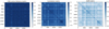 |
Fig. 1 Matrices showing pairwise comparison between frames, computed using different image comparison methods, where the x and y axes correspond to the index of a single frame from the master reference library. |
3.1 Image comparison methods
The image comparison methods we studied were the cosine distance, using a convolutional neural network (CNN), the Pearson correlation coefficient, and the structural similarity index measure (SSIM). Using each of these methods, we computed a comparison matrix of dimensions N × N, where N = 19 695 = total number of science frames in our master reference library, and where each row and corresponding column with the same index represents a specific frame of a science cube. Each cell in the matrix will then contain the result of a given method applied between the two frames it represents.
3.1.1 Convolutional neural network
Thanks to technological progress and the ability to performtime-consuming calculations, artificial intelligence (AI) has seen great advances in recent years. Besides its numerous applications in industry, it is becoming increasingly used in astronomy, namely to simulate, identify, and classify objects (Yip et al. 2019; Jia et al. 2020; Ethiraj & Bolla 2022; Guo et al. 2022).
Acknowledging the established efficacy of wavelet techniques (Starck & Murtagh 1993), our study adopts a deliberate pivot toward investigating the utility of a CNN. This exploration is motivated by a scientific inquiry into the potential advantages that CNNs, known for their deep learning capabilities, may offer.
We chose a CNN called Resnet 50 (He et al. 2015), which is a deep-learning algorithm that is 50 layers deep and pre-trained with the ImageNet1 data set. This data set comprises more than 1.2 million images, allowing us to identify patterns, classify up to 1000 different classes, and extract the main characteristics of the images.
Throughout the learning process, multiple convolutions culminate in the penultimate layer of our Convolutional Neural Network, which produces a one-dimensional descriptor for each image, encapsulated in a 2048-element vector. While these vectors may not be traditional basis vectors, they fulfill a comparable role, offering a compact yet richly expressive representation of the image data.
The physical significance of these basis vectors lies in their capacity to represent the complex, high-dimensional data in a form amenable to comparison and analysis. They capture the essential information that differentiates one image from another while discarding noise and redundant data.
In our methodology, we consciously bypass the network’s final, fully connected layer – typically responsible for classifying images into predetermined categories – as our focus diverges from classification. Instead, our interest lies in the nuanced feature extraction applicable to the entire SHARDDS data set, resulting in the generation of 19 695 unique descriptors. These descriptors form the basis of our reference library, established through the computation of cosine distances between each descriptor pair. This computation hinges on the measurement of the angular difference between vectors, as delineated in Eq. (1). The culmination of this process is a similarity matrix, depicted in Fig. 1, where a cosine value of 1 denotes the highest degree of similarity (the closest match) between images and a value of −1 indicates the least similarity (the farthest match) to the reference image:
 (1)
(1)
where A and B represent two image descriptors, while ‖A‖ and ‖B‖ represent the L2-norm of vectors A and B, respectively.
3.1.2 Pearson correlation coefficient
For the correlation method, we flattened the pixels of each image from our master reference library (199 × 199 pixels) into a single column of 39 601 elements for a total of 19 695 frames. With this resulting matrix, we were able to compute the Pearson correlation coefficient (PCC) showing the linear dependency between the frames, with values from 1 to −1, where 1 is the most correlated, according to Eq. (2):
 (2)
(2)
here, Xi and Yi are the reference frames and  and
and  are the means of those frames. The resulting correlation matrix is shown in Fig. 1 (middle image).
3.1.3 Structural similarity image index
Another image comparison method is the structural similarity image index (SSIM) (Wang et al. 2004), specifically the implementation provided by the skimage.metrics.structural_ similarity Python library (van der Walt et al. 2014), which returns the mean structural similarity index over the image calculated using Eq. (3). This method was also used in the study of Ruane et al. (2019). Similarly to the previous methods, we considered each science image and computed the SSIM index against all other images in the master reference library, creating a matrix with the results:
 (3)
(3)
where Npix is the number of pixels in the comparison region (in our case, 199×199 pixels for a full-frame image); L, C, and S are the luminance, contrast, and structural terms, respectively; and i [1, Npix] is the pixel index. Luminance comparison involves assessing the average brightness between images. Contrast comparison examines the variability in pixel intensities, reflecting the texture and depth. Structure comparison examines pattern similarities, ensuring that the spatial relationships among pixels are preserved.
As shown in Fig. 1, the three matrices have different values depending on the metrics used. A comparison between them to study their level of sensitivity is done in Appendix A.1 (the complete appendix is available at Zenodo; see link in Section 6).
3.1.4 Environmental variables and Strehl ratio
To identify the environmental variables that describe image quality and enable frame selection without additional calculations, we analyzed their effects using metadata information (e.g., adaptive optics telemetry information, wind speed at 30 me, coherence time, seeing…). Understanding the impact of these variables on contrast will help to determine the most effective metric for this purpose. Further details are provided in Appendix B.
The environmental variables are read from sensors located in the meteorological tower at the Paranal Observatory, as well as from the data obtained from the SPHERE Standard Platform for Adaptive Optics Real Time Applications (SPARTA, Suárez Valles et al. 2012). These values are stored every 20 seconds in a file that is available in the European Southern Observatory (ESO) archive. Appendix B.1. shows a histogram of the most relevant environmental variables in the master reference library. Table 1 lists the environmental variable values for HD 206893 and the three best targets with the best S/Ns.
The Strehl ratio (SR), which is the ratio of the peak intensity of a measured point spread function (PSF) to the peak intensity of a perfect diffraction-limited PSF for the same optical system, is widely used to measure the performance of an adaptive optics system (Roberts et al. 2004). The SPARTA real-time computer system estimates the Strehl from closed-loop slope measurements (Fedrigo et al. 2010), which is particularly useful when the observed star is masked by a coronagraph.
This calculation process begins with the projection of the residual slopes, denoted as sn, onto the Karhunen–Loève (KL) mode basis (Fukunaga & Koontz 1970). This projection is analogous to the method used for estimating turbulence parameters and results in the KL coefficients of the residual slopes, denoted as  and computed as
  , where S2M is the projection matrix on a KL basis. Following this, the temporal variance of these coefficients,
  , is computed. The noise variance for each mode,
  , is then deducted from the corresponding temporal variance:
 (4)
(4)
The total residual variance is calculated by summing the residual variances  for each KL mode, which are weighted by the square of the ratio of the imaging wavelength (λim) to the wavefront sensor wavelength (λwfs). This process can be mathematically expressed as follows:
 (5)
(5)
The fitting error, denoted  , is calculated using Fried’s r0, and follows the following formula:
 (6)
(6)
where D is the telescope’s diameter and λim is the imaging wavelength.
Finally, SR is computed as the exponential of the negative sum of the total residual variance and fitting error:
 (7)
(7)
According to Serabyn et al. (2007), SR directly impacts the raw contrast level C through the rule of thumb C ∝ (1-SR)/N2 with N2; this is the number of AO correcting elements (~ 1300 in SAXO). Raw contrast refers to the ratio between the peak brightness of the central star and the brightness of the faintest point in the image that can still be discerned. It represents the primary level of contrast discernible by the imaging system before any post-processing techniques such as RSDI or ADI are applied. To explore this relationship further, we systematically collected the values of environmental variables for each science image and computed their raw contrast at a separation of 245 mas. This approach enables us to use contrast as a comparable metric and thus verify whether there is a linear relationship between the environmental variables and the raw contrast at the given separation.
Because our master reference library includes several frames from the same object, many of the contrast values are very similar. Therefore, we grouped these values into percentiles of 25, 50, and 75 to calculate the Pearson correlation between contrast and each of the environmental variables. Organizing data into percentiles does not involve assigning different weights to individual data points. Instead, it serves to pinpoint specific values at predetermined positions within the data set, effectively dividing it into segments. Our analysis confirmed that the SR was the most correlated variable. As the SR increases, the value of the contrast improves, and there is an inverse correlation with the Pearson correlation coefficient of −0.73 (see Appendix B.2).
To corroborate these results, we used a machine learning decision-tree-classifier algorithm (Pedregosa et al. 2011), separating 70% of our environmental variables and contrast data for the training of the algorithm and 30% for validation. Considering that we wanted to obtain values within the percentiles explained previously, applying our algorithm gave us an acceptable precision of 0.86. A precision of 0.86 means that when the model predicts a certain outcome, it is correct 86% of the time. This level of precision is generally considered good and suggests that the model is a reliable tool for evaluating the relationship between the contrast of an image and the measured environmental variables Hastie et al. (2009). By calculating the feature importance (Appendix B.3), we established that the SR is the environmental variable with the greatest significance in predicting contrast outcomes.
Based on these findings, we created a comparison matrix containing the absolute difference between the SR from each frame and the rest of the data set.
Environment variable values for HD 206893 (our science target); HD 3003, HD 105, and HD 9672; the three targets with the best S/N using single full-frame RSDI-PCA; and HD 82943, the target with the worst result.
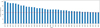 |
Fig. 2 X-axis shows ID of frames included in the reference library of HD 206893 using the PCC metric. The Y-axis shows the number of times a given reference frame is among the top R=25 most similar frames when considering all the 576 scientific frames of HD 206893. A threshold N=50 (red line) was used to build the reference library; we therefore only show the reference frames present more than 50 times in the top 25 most similar frames here. This criteria (R=25, N=50) is relatively restrictive in this example, as we end up with only 36 frames in the reference library. |
3.1.5 Raw-contrast criteria
Because the raw contrast (RC) is related to (1-SR), the idea is to identify or corroborate whether there is any difference by using this metric instead of the SR itself. Typically, a 1% decrease in the Strehl ratio does not make much of a difference; however, it has a significant impact when (1-SR) increases from 1% to 2%. Moreover, the actual intensity in the stellar residual halo is usually not the biggest problem for detecting faint objects, the temporal/spatial variations are. (Gladysz et al. 2008).
To address this, we created a comparison matrix containing the absolute difference between the raw contrast from each frame and the rest of the data set, similarly to the SR analysis. Specifically, we used raw contrast at a separation of 245 mas as a metric.
3.2 Selection of a reference library for a given science target
For a given similarity metrics, two different strategies can be implemented. We can optimize the reference library per scientific frame or per scientific target, meaning there will be a unique reference library valid for all the scientific frames of this observation. The former was implemented by Xie et al. (2022) and Ruane et al. (2019) and is more computationally intensive because there are as many reference libraries as scientific frames. We tested both techniques and showed that the latter yielded a higher signal-to-noise ratio on HD 206893 B. This technique is therefore considered as our baseline. The comparison of the two strategies is discussed in Section 5.
With a unique library per scientific observation, we now explain the selection criteria to determine whether or not a given frame from the master reference library belongs to the optimized reference library for a given target, in our case HD 206893.
3.2.1 Definition of the selection criteria (R,N)
After obtaining a comparison matrix for each image comparison method (Fig. 1), the next step was to find a suitable subset of frames, similar to the set of science frames, to be included in the reference library. For this purpose, we applied the following criteria: a frame would be selected for the reference library if it appeared at least R times among the N “closest” frames to our science frames, where R is an integer with a maximum range between 1 and the number of science frames, and N is an integer with a maximum range between 1 and the total number of frames from the master reference library after excluding our science target.
For each frame of our science target, we wanted to explore N ranging from 25 to 100, which was selected because the reference cubes that can be formed depending on the combination of R and N can vary between 1169 and 4221 frames as maximum values. Taking values greater than 100 would create very large reference cubes, and it would consume considerable computational power to apply RSDI-PCA and be capable of considering all the numbers of components for the reduction algorithm.
From the resulting set of “closest” frames, we iteratively explored a range of R from 1 to 50, incremented in steps of 5. This should allow us to achieve a more balanced distribution, selecting frames that were not only strongly similar to one of the science frames, but also to several of them. Fig. 2 shows the total number of occurrences within the top 25 for each of the selected frames of an example reference library created with N=25 and R=50. Table 2 shows a summary of the different methods with criteria R and N versus the number of components and the size of the images.
Parameter space explored.
3.2.2 Specific case for (R,N)=(1,1)
Additionally, we created a reference library by selecting the closest frame to each frame of our science target; that is, N=1 and R=1. This leads to a relatively small reference library, consisting of a maximum number of frames equal to the number of science frames (if every single frame is best correlated to a distinct reference frame), but it is usually smaller than this number.
3.2.3 Random selection
To corroborate that our methods deliver meaningful results, we created reference libraries by selecting 250, 500, and 750 random frames from our master reference library, and we repeated this process 100 times for each of these library sizes. As explained in Section 3.2, we did not consider frames belonging to our science target.
In a set of 19 695 frames, the number of 750-combinations is  , therefore testing all those possibilities to find the best library out of all possible libraries of 750 frames is not computationally tractable. Instead, we restricted ourselves to 100 random draws; this allowed us to determine the best possible performance if one could afford 100 draws of random libraries, noting that the probability of obtaining the best library by chance in these 100 draws is 100 : 10723 261.
3.2.4 No selection: Using the complete master reference library
As another benchmark to observe the impact of frame selection, we also considered the complete master reference library without any filtering (e.g., the 19 119 images).
3.3 Limiting to an area of interest of 6–15λ/D
The area we want to consider to understand how RSDI performs ranges from 6λ/D to 15λ/D, or from 245 to 612 mas. Because ADI has some limitations under 300 mas, we chose an inner radius slightly below to verify if our method is a good alternative. More importantly, HD 206893 B has been detected at separations of 270.4 mas (Romero et al. 2021). The outer radius was chosen such that our area of interest would remain within the correction zone of SPHERE’s adaptive optics system, 20λ/D.
To verify whether there is any difference between executing the aforementioned procedures on the full-frame (199 × 199 px) image and restricting them to this specific zone, we limited each of our science frames to an annulus covering the same area, corresponding to 20–50 pixels as the inner and outer radii, respectively. We then created new reference libraries (see Fig. 3), which we used to perform a PCA and compare the results with the full-frame image libraries in terms of S/N on the companion HD 206893 B.
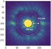 |
Fig. 3 Science image of HD 206893. Our area of interest is delimited by the dashed circles; it ranges from 20 to 50 pixels, corresponding to 245 to 612 mas and 6λ/D to 15λ/D, which is within the correction zone of the SPHERE adaptive optics system, 20λ/D. |
3.4 Detector integration time influence
To determine if there is any relation between detector integration time (DIT) and image similarity, thereby contributing to the selection of frames for the creation of the reference library, we first looked at the initial distribution within the master reference library. The most frequent DIT was 4s for 38% of the data, followed by 8s for 25%, 16s for 20%, 2s for 12%, and 32s for 4% of the data. Fig. 4 shows a histogram of the DIT distributions.
Our science target has a DIT of 4s. However, our similarity-based libraries are not only composed of 4s DIT frames, they also follow a distribution similar to that of the master reference library. Therefore, we expect that most libraries are composed of frames taken with DITs of 4s that do not necessarily present any relation to the DIT of the science frames.
3.5 Spectral type distribution and relevance
The SHARDDS survey examines a broad spectrum of spectral types and ages from A to M and has ages ranging from 10 Myr to 6 Gyr (Dahlqvist et al. 2022), noting the potential effects of spectral type on diffractive halos, a concept referenced by Gray & Corbally (2009). However, this study prioritizes the enhancement of the detection sensitivity for companions close to bright stars. It employs a reference image library, chosen through various similarity metrics, aiming for a comprehensive assessment across the survey without any specific pre-selection based on spectral types.
To understand if there is any strong relation with our science target, the F5V star HD 206893, we first analyzed the distribution of frames across different spectral types. Spectral type F was the most prevalent, comprising 7,599 frames (38.58% of the total). This was followed by spectral type A with 5,810 frames (29.50%) and spectral type G with 4124 frames (20.94%). Spectral type K accounted for 1778 frames (9.03%), whereas spectral type B had 240 frames (1.22%). Spectral type M had the least representation, with 144 frames (0.73%). This distribution highlights the dominance of F-type stars in the data set, followed by A- and G-type stars, indicating a preference for these types. If there is a strong influence, we can expect most libraries yielding the best results to be created with F-type stars. The distribution is shown in Fig. 5.
 |
Fig. 4 Histogram showing number of frames per DIT of master reference library (orange) and reference library created using the correlation method with N = 50 and R = 10 (blue). This reference library contains 601 frames, with 50.3% having a DIT of 4s, 28.7% having a DIT of 16s, and 15.8% having a DIT of 8s. Despite the science target’s DIT being 4s, the reference library was created with a broader range of DITs. |
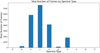 |
Fig. 5 In the histogram showcasing spectral types, type F stands out with the highest frequency, constituting 7599 out of the 19 695 frames; this represents approximately 38% of the entire program. |
4 Data reduction and metrics for performance assessment
To evaluate if the introduction of our reference libraries effectively improves the robustness of planet detection, we used the S/N and contrast curves measured on our reduced images as metrics. Our images were reduced following different techniques to have a point of comparison for our methodologies, as detailed in the following subsections.
4.1 Data reduction
Our data were reduced in classical ADI (cADI), ADI-PCA, and RSDI-PCA. The RSDI was first applied to our science image, HD 206893, considering as reference cube each of the other targets in our master reference library, which we have defined as single RSDI-PCA, and then each of our reference libraries. When applying the PCA, the number of principal components we considered for ADI ranged from 10 to 40, incrementing in steps of ten; and for RSDI from ten up to the total number of frames of the reference cube, incrementing in steps of 20.
For this purpose, we used the Vortex Image Processing package (VIP; Gomez Gonzalez et al. 2017). VIP is a Python package for angular, reference star, and spectral differential imaging for exoplanet and disk high-contrast imaging. The normalization methods offered by this package that we applied to our PCA and during this procedure are applied to both the science cube and the reference library were “none”, “temp-mean” and “spat-mean”. With “none”, no scaling is performed on the input data; with “temp-mean”, the temporal mean subtraction is done; and with “spat-mean”, the spatial mean is subtracted. Using the temp-mean normalization is equivalent to performing a cADI reduction prior to applying the RSDI reduction; therefore, it is subject to self-subtraction as in any ADI algorithm.
4.2 Signal-to-noise ratio and contrast curve
One of the metrics that we considered to measure the performance of our libraries is the S/N, calculated using VIP, which uses the definition given in Mawet et al. (2014):
 (8)
(8)
where  is the flux measured at the potential companion;
  is the mean of the flux measured in the resolution elements used (excluding the potential companion), which are located at the same radial distance as
  is the standard deviation of these elements; and n2 is the number of apertures used at that particular separation. Each of these resolution elements, or apertures, has a radius of FWHM/2, and their number depends on the distance from the center of the image and the full width at half maximum (FWHM) used.
In addition, we considered the contrast curves as a metric, since they are widely adopted as a measure to determine the star-planet ratio. Even though contrast curves have some limitations (Jensen-Clem et al. 2018), we consider them sufficient, together with the S/N, to perform a relative comparison between algorithms.
The contrast was calculated according to Eq. (9):
 (9)
(9)
where F is a multiplicative number, in our case with the value five in order to generate a 5σ contrast curve, N is the standard deviation of the annulus with an aperture of FWHM, Tr is the ratio between the flux of the injected fake companion recovered after the post processing algorithm was applied and the flux of the fake planet initially injected, and Sp is the total flux measured on the point spread function (Jensen-Clem et al. 2018; Gomez Gonzalez et al. 2017). Given the separations at which HD 206893 B was detected, the values presented in Section 5 correspond to the mean contrast between 245 and 275 mas.
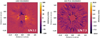 |
Fig. 6 Science images after performing cADI on the left and ADI-PCA on the right. The S/N measured in cADI is 2.2, and in ADI-PCA it is 7.3, with 40 principal components removed. Such a low value in cADI is considered as a non-detection. |
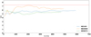 |
Fig. 7 Graph shows evolution of S/N of three best performing objects vs. the number of principal components (ncomp). The best value is observed when RSDI-PCA is performed with HD 3003 as reference star using 210 principal components. The dashed line represents the S/N obtained with ADI-PCA, 7.3. |
5 Results
The S/N obtained for HD 206893 using the cADI was 2.2. For ADI-PCA, the best full-frame result is an S/N of 7.3 with a contrast of 3.74 × 10⁻⁵, considering 40 principal components (see Fig. 6). With the optimization zone described in 3.3, the best S/N value is 8.0 with a contrast of 2.77 × 10⁻⁵, using 10 principal components.
When performing a single RSDI-PCA between all SHARDDS objects and our science target HD 206893, there was no improvement in terms of S/N with respect to ADI-PCA. Fig. 7 shows the evolution of the S/N with respect to the number of principal components for the three best references. The best and worst results are presented in Table 1. The best S/N (full frame) is 7.2 with a contrast of 3.93 × 10⁻⁵; we used HD 3003 as a reference target and 210 principal components. This object was observed the night before our science cube, and the closest object in terms of time was HD377, which was observed on the same night and immediately after. However, it has an S/N of 5.3, which indicates that an object on the same observing night will not necessarily show the best performance. The second best result we obtained was using HD 105 as the reference target and 400 principal components, offering an S/N of 5.9 and a contrast of 3.80 × 10⁻⁵ (see Fig. 8). With the optimized zone, the maximum S/N was 6.8 with a contrast of 4.22 × 10⁻⁵; we used HD 15257 as the reference and 410 principal components.
All of these results, including those obtained with our reference libraries, use temp-mean when applying PCA. From the different normalization (or scaling) methods offered by VIP that we tested (Section 4), we find that temp-mean produces the best results (see Figs. D.1 and D.2 in the appendix), which is equivalent to performing a cADI reduction prior to applying RSDI reduction.
When evaluating the performance of our reference libraries, we calculated the average value of the ten best libraries built according to each method to cope with possible outliers and acquire a better perspective of their overall behavior. We grouped our results using an image comparison method; we made selections according to our criteria (with R>1, N>1 and R=1, N=1) and random selection, with and without the optimized zone (full-frame).
For CNN, the average of the ten best libraries results in an S/N of  , with a corresponding average contrast of 3.73 × 10⁻⁵. With the optimized zone, the values are an S/N of
  with a contrast of 3.96 × 10⁻⁵, which is the average of the ten best results.
According to our findings, PCC is the image comparison method with the best overall performance. The average S/N value of this method within the top ten results is  , with an average contrast of 2.61 × 10⁻⁵, which is better than all the results using a single RSDI-PCA with the SHARDDS data set and also better than cADI and ADI-PCA. The reference library with the best (full-frame) result,was created using 70 principal components (N=50 and R=10) with a total of 601 frames (Fig. 9).
When applying the optimized zone, we obtained an average S/N of  , with a corresponding average contrast of 2.58 × 10⁻⁵, and the maximum S/N value was obtained with N=50 and R=40, using a total of 233 frames and 150 principal components. This is our absolute best result amongst all the reference libraries we created (Fig. 10), with a contrast value of 2.48 × 10⁻⁵.
Figure 11 shows the S/N achieved with all the reference libraries created using the PCC method with the optimized zone. We can see that 11 libraries generate better results than ADI-PCA and RSDI-PCA in full-frame, and seven libraries were above eight, which is the best S/N obtained with ADI-PCA with an optimized zone.
Using SSIM, the average S/N value of the ten best libraries created with SSIM was  , with an average contrast of 3.21 × 10⁻⁵. When applying the optimized zone, we have an average S/N of
  , with an average contrast of 2.62 × 10⁻⁵. The maximum value was delivered by the library created with N=75, R=45, and 70 principal components, with a total of 317 frames. Therefore, there is a performance improvement of 23% as a result of this optimization zone.
With Strehl, the average of the ten best libraries is  , with an average contrast of 2.90 × 10⁻⁵. With the optimized zone, the average S/N of the ten best libraries is
  , with an average contrast of 3.02 × 10⁻⁵.
As confirmed in Section 3.1.4, Strehl is an important variable in relation to contrast. Nevertheless, Table 1 shows both the three targets offering the best S/N when used as reference in a single RSDI-PCA and HD 82943 (Figs. 12 and 13), the target with the worst S/N (0.8); they share a Strehl value quite similar to our science target, HD 206893.
Figure 14 shows the S/N as a function of the Strehl ratio for the entire master reference library. Most of the points within ± 10% of the Strehl ratio of HD 206893, 0.84, are above the average S/N. However, seven objects did not follow this trend, representing 28% of our results within these tolerance limits. This means that, while in most cases a good S/N is associated with a corresponding good Strehl ratio value, there are cases where the S/N result is even below the mean at a similar Strehl ratio.
Therefore, although the Strehl ratio can be used to select similar images, it is not a sufficient metric that can be used on its own, as seen in Appendix B.4. There are other effects that produce a bad reference image quality in comparison to our science image that are not detected by strictly analyzing the Strehl, such as bad coronagraph centering, the low-wind effect (LWE; Milli et al. 2018), or the wind-driven halo effect (Cantalloube et al. 2018, 2020).
Using the raw contrast as a metric, the average of the ten best libraries was  . With the optimized zone, the average S/N of the ten best libraries was
  , with an average contrast of 3.45 × 10⁻⁵. These results suggest that raw contrast alone is not sufficient for selecting reference images due to potential asymmetries, such as the wind-driven halo effect, which can impact image quality. Similarly, the Strehl ratio cannot be used as the sole metric for similar reasons.
When selecting the specific case (N=1, R=1), the best result was obtained using the correlation method; the average of ten the best libraries delivered an S/N of  , with an average contrast of 3.06 × 10⁻⁵. Moreover, the best value using 50 principal components and a total of 134 frames were used. With the optimized zone, the average of the ten best libraries is an S/N of
  , with an average contrast of 2.57 × 10⁻⁵.
Using random selection, the average S/N of the ten best libraries was  , with an average contrast of 2.67 × 10⁻⁵. When applying the optimized zone, we also obtained an average S/N of
  and an average contrast of 2.80 × 10⁻⁵. 5.1% of the S/N values from the random selection results were above the best values of ADI-PCA and the single RSDI-PCA, which highlights the efficacy of conventional algorithms (see Fig. 15). However, if we analyze the total histogram of single RSDI-PCA and random selection (Fig. 16), we see that the latter performs much better, which shows us that the diversity of images in the reference cube makes our S/N better than choosing the single RSDI strategy.
A summary of these results is presented in Table 3.
As described in Section 3.2.4, we used the SHARDDS master reference library for comparison, with both the full frame and an optimized zone constituting our reference cube. However, this method did not yield significant results, with the highest S/N reaching only 4.1 using 100 principal components, and an average top ten S/N value of 2.4. The progression of these calculations is detailed in Appendix C.2.
Now, when comparing the results obtained with our method versus the method used in Ruane et al. (2019), with respect to the selection by frame, the best result was obtained as a full-frame S/N of 5.6; with an optimized area, it was S/N 4.0. The best results are obtained by making a reference library by cube and then making a grid search with the respective numbers of principal components as explained in Section 3.2.1
Concerning the variation of the number of principal components when applying PCA, we did not observe a well-defined trend. However, we verified that the S/N varies according to the number of principal components considered. Therefore, in order to optimize this value and find the optimum number of components, we must start with a low number and progressively increase it until a maximum equal to the size of the library is reached.
The efficacy of our reference libraries was evaluated in relation to the spectral type of the stars. We analyzed the distribution and relevance of these spectral types, as illustrated in Appendix E. Analysis of the top ten libraries using PCC indicates that G-type stars are more frequently represented than F-type stars. Additionally, a cube made up of frames exclusively from F-type stars within the optimized area, comprising 5, 727 frames, achieved an S/N of 5.2 with 250 principal components, which is lower than the results obtained using PCC. Despite SHARDDS being predominantly based on F-type spectral data, the libraries yielding the highest S/Ns exhibited a more significant contribution from G-type stellar frames (54%) compared to F-type frames (25%). This suggests that the data set performs better in RSDI when encompassing a broader array of spectral types rather than being overly concentrated on F-type stars, such as the spectral type associated with HD 206893.
 |
Fig. 8 Images offering best results after performing RSDI-PCA on HD 206893 with all the SHARDDS library. On the left, the reference target is HD 3003 and on the right HD 105, with an S/N of 7.2 and 5.9, respectively. |
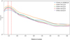 |
Fig. 9 5-σ contrast curve. RSDI-PCA with correlation library (blue line) shows a better behavior than with ADI (red, green, and yellow lines); this corresponds to the components we used within this method. The library has 601 frames and it was created with N=50 and R=10, considering 70 principal components when applying the PCA. The contrast achieved with this library is 2.48 × 10⁻⁵ between 245 and 275 mas. |
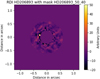 |
Fig. 10 Final image reduced with RSDI-PCA offering best S/N results. It was obtained from images with an optimized zone using the correlation method with N = 50, R = 40, and 150 principal components. |
 |
Fig. 11 Box plot shows S/N obtained with all the reference libraries created with the correlation method using the optimized zone, identified in the x-axis by the respective N and R values (in the format N_R). The horizontal lines indicate the best S/N achieved with the ADI-PCA full-frame (red dashed line) and optimized zones (orange line), and the single RSDI (green dashed line) and optimized zones (blue line). The maximum S/N value is 9.1, achieved with N=40 and R=50. |
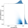 |
Fig. 12 Strehl difference matrix as a function of correlation matrix, showing that the highest density of points is found when there is a low difference between the Strehl values and a high correlation of the images. However, there are also cases where the Strehl difference is low, but the correlation value is decreasing. This means that for this data set, Strehl is not a good comparison metric. |
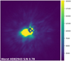 |
Fig. 13 Image of HD 82943 delivering the worst S/N when performing RSDI-PCA with HD 206893, even though their Strehl values are similar. Therefore, Strehl cannot be used as a reliable representative of the image quality encompassing all its parameters. |
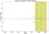 |
Fig. 14 S/N as function of Stгehl ratio for the entire master reference library. The black line along the x-axis indicates the mean Strehl ratio value of 0.78. Along the y-axis, the black line represents the mean S/N obtained with single RSDI-PCA on all SHARDDS objects. The blue segmented line is the Strehl ratio value of HD 206893, 0.84, and the yellow area marks ± 10% tolerance limits with respect to this value. |
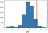 |
Fig. 15 Histogram of S/N from random selection (full-frame). The red line indicates the best S/N obtained when performing single RSDI, and the black line shows the best S/N in ADI-PCA. We note 5.1% of the S/N values are above the results obtained with these two methods. The blue line is the best S/N value obtained with the correlation method with an optimized region. |
Summary of best S/N results for each of the different image comparison and selection methods: full-frame and with the optimized zone.
6 Concluding remarks and perspectives
In this study, we used the IRDIS data from the SHARDDS survey to investigate the performance of the RSDI depending on the frame selection strategy. Our performance indicator was the S/N obtained on the low-mass companion HD 206893B, detected at 270 mas with a contrast of 11.1 mag. As a benchmark for comparison against our RSDI-PCA methods, the ADI-PCA yields an S/N of 7.3. After investigating the various RSDI normalization options offered by VIP, we find that temp-mean performs the best.
Reducing HD 206893 with a single RSDI-PCA, using each target of our data set as a reference, showed the best S/N value of 7.2 with the target HD 3003. Thus, ADI-PCA delivers better results than RSDI-PCA using SHARDDS objects without library optimization.
The best frame selection technique is the PCC applied to an annulus between 245 and 610 mas, yielding a, S/N of  . With the optimized zone, we verified that 11 of those libraries achieved an S/N above ADI-PCA and RSDI-PCA with each target as the reference full frame, and seven libraries above 8.0, which is the best S/N obtained with ADI-PCA with the optimized zone.
The adopted CNN does not deliver better values than traditional methods. One reason for this may be that it is a pre-trained CNN, without astronomical images similar to SPHERE’s for training. Despite these results, the possibility of improving the performance of RSDI using artificial intelligence should not be excluded. A possible approach might be to train a CNN specifically with SPHERE data to determine if this improves image selection, thereby delivering a better S/N than the PCC or SSIM.
Our research has shown that both the Strehl ratio and raw contrast are important metrics for evaluating the performance of instruments utilizing adaptive optics (AO) systems. These metrics are used to assess image quality and contrast. However, our findings suggest that relying solely on the Strehl ratio to select reference images is insufficient. The Strehl ratio does not account for certain asymmetries and artifacts in the raw images, such as poor centering of the coronagraph, background emissions, aberrations, low wind effect, and wind-driven halo effect. Similarly, raw contrast is not the best metric because its calculation can be influenced by these asymmetries. These limitations are not unique to the SHARDDS data set; rather, they are inherent characteristics of the SPHERE AO system, irrespective of the specific observational circumstances. Therefore, these considerations must be taken into account when selecting reference images, as using only these two metrics as the primary criteria for image selection is insufficient.
Our evaluation of reference libraries in relation to spectral types revealed that G-type stars are more prevalent in top-performing libraries than F-type stars. A reference cube solely from F-type stars achieved a lower S/N (5.2 with 250 principal components) compared to PCC results. Despite SHARDDS’s dominance of F-type stars, the highest S/Ns were from libraries with more G-type (54%) than F-type (25%) frames. This suggests that, in this particular case, varied spectral types improve RSDI performance rather than focusing solely on F-type stars.
Using random images, we were able to find that image diversity in the reference cube generates a better result than using a single RSDI-PCA. This is very important as it indicates that, in this particular case, it is better to generate a library of different frames belonging to different objects than to use an individual target as a reference frame. Furthermore, the random selection method performs very well compared to our other methods, being outperformed by the PCC method, which performs better considering both the S/N and the computation time required to arrive at the results.
Among all our methods, we found that the version with an optimized zone provides a similar or better result than using the full frame. This is because it allows us to evaluate the image similarity strictly within the area of interest where we might expect planet detection, while discarding areas of the image that do not contribute to our investigation. We also verified that the number of principal components we use when computing the PCA affects the S/N, although we cannot identify a well-defined pattern.
As a future perspective, we intend to apply the PCC method in an optimized area as a selection strategy to reprocess all data available in the SPHERE Data Center. This approach is aimed at searching for faint planets that may previously have been undetected by less sensitive techniques. However, we acknowledge the need for further testing on additional targets before generalizing our findings. Stasevic et al. (in prep.) will assess these results using a broader data set and a different filter (narrowband H23) to provide further validation.
 |
Fig. 16 RSDI – PCA S/N density curve after having used the whole data set of SHARDDS per object; the Sthгel variable and the image similarity methods; and comparing it with the S/N values provided by the random selection (in green). The black curve corresponds to the full-frame method, the blue one to the optimization-zone method, and the green one to the random distribution; the dotted line corresponds to the maximum values per curve. The best performance is provided by the correlation with a median of 6.2 and a maximum S/N value of 9.1. |
Data availability
The complete appendix is available at https://doi.org/10.5281/zenodo.13647358
References
- Amara, A., & Quanz, S. P. 2012, MNRAS, 427, 948 [Google Scholar]
- Beuzit, J.-L., Vigan, A., Mouillet, D., et al. 2019, A&A, 631, A155 [NASA ADS] [CrossRef] [EDP Sciences] [Google Scholar]
- Bohn, A. J., Kenworthy, M. A., Ginski, C., et al. 2020, ApJ, 898, L16 [Google Scholar]
- Bohn, A. J., Ginski, C., Kenworthy, M. A., et al. 2021, A&A, 648, A73 [NASA ADS] [CrossRef] [EDP Sciences] [Google Scholar]
- Cantalloube, F., Por, E. H., Dohlen, K., et al. 2018, A&A, 620, L10 [NASA ADS] [CrossRef] [EDP Sciences] [Google Scholar]
- Cantalloube, F., Farley, O. J. D., Milli, J., et al. 2020, A&A, 638, A98 [NASA ADS] [CrossRef] [EDP Sciences] [Google Scholar]
- Choquet, É., Pueyo, L., Soummer, R., et al. 2015, SPIE Conf. Ser., 9605, 96051P [NASA ADS] [Google Scholar]
- Choquet, É., Perrin, M. D., Chen, C. H., et al. 2016, ApJ, 817, L2 [NASA ADS] [CrossRef] [Google Scholar]
- Choquet, É., Milli, J., Wahhaj, Z., et al. 2017, ApJ, 834, L12 [NASA ADS] [CrossRef] [Google Scholar]
- Choquet, É., Bryden, G., Perrin, M. D., et al. 2018, ApJ, 854, 53 [Google Scholar]
- Dahlqvist, C.-H., Milli, J., Absil, O., & Cantalloube, F. 2022, A&A, 666, A33 [NASA ADS] [CrossRef] [EDP Sciences] [Google Scholar]
- Delorme, P., Schmidt, T., Bonnefoy, M., et al. 2017, A&A, 608, A79 [NASA ADS] [CrossRef] [EDP Sciences] [Google Scholar]
- Dohlen, K., Langlois, M., Saisse, M., et al. 2008, Proc. SPIE, 7014, 851 [Google Scholar]
- Ethiraj, S., & Bolla, B. K. 2022, arXiv e-prints [arXiv:2205.07124] [Google Scholar]
- Fedrigo, E., Bourtembourg, R., Donaldson, R., et al. 2010, in Adaptive Optics Systems II, 7736, eds. B. L. Ellerbroek, M. Hart, N. Hubin, & P. L. Wizinowich, International Society for Optics and Photonics (SPIE), 77362I [NASA ADS] [CrossRef] [Google Scholar]
- Fukunaga, K., & Koontz, W. 1970, Inform. Control, 16, 85 [CrossRef] [Google Scholar]
- Gerard, B. L., & Marois, C. 2016, SPIE Conf. Ser., 9909, 990958 [Google Scholar]
- Gladysz, S., Christou, J. C., Bradford, L. W., & Roberts, L. C. Jr. 2008, PASP, 120, 1132 [NASA ADS] [CrossRef] [Google Scholar]
- Gomez Gonzalez, C. A., Wertz, O., Absil, O., et al. 2017, AJ, 154, 7 [Google Scholar]
- Gray, R. O., & Corbally, C. J. 2009, Stellar Spectral Classification, Princeton Series in Astrophysics (Princeton University Press) [CrossRef] [Google Scholar]
- Guo, Z.-X., Yang, J.-Y., Dunlop, M., et al. 2022, J. Atmo. Solar-Terrestrial Phys., 235, 105906 [NASA ADS] [CrossRef] [Google Scholar]
- Hastie, T., Tibshirani, R., & Friedman, J. 2009, The Elements of Statistical Learning: Data Mining, Inference, and Prediction, 2nd edn. (Springer) [Google Scholar]
- He, K., Zhang, X., Ren, S., & Sun, J. 2015, arXiv e-prints [arXiv:1512.03385] [Google Scholar]
- Hinkley, S., Lacour, S., Marleau, G. D., et al. 2023, A&A, 671, L5 [NASA ADS] [CrossRef] [EDP Sciences] [Google Scholar]
- Hunziker, S., Schmid, H. M., Ma, J., et al. 2021, A&A, 648, A110 [NASA ADS] [CrossRef] [EDP Sciences] [Google Scholar]
- Jensen-Clem, R., Mawet, D., Gomez Gonzalez, C. A., et al. 2018, AJ, 155, 19 [Google Scholar]
- Jia, P., Liu, Q., & Sun, Y. 2020, AJ, 159, 212 [NASA ADS] [CrossRef] [Google Scholar]
- Lawson, K., Currie, T., Wisniewski, J. P., et al. 2022, ApJ, 935, L25 [NASA ADS] [CrossRef] [Google Scholar]
- Marois, C., Lafrenière, D., Doyon, R., Macintosh, B., & Nadeau, D. 2006, ApJ, 641, 556 [Google Scholar]
- Marshall, J. P., Milli, J., Choquet, É., et al. 2018, ApJ, 869, 12 [Google Scholar]
- Marshall, J. P., Milli, J., Choquet, E., et al. 2023, MNRAS, 521, 5940 [CrossRef] [Google Scholar]
- Mawet, D., Milli, J., Wahhaj, Z., et al. 2014, ApJ, 792, 97 [Google Scholar]
- Milli, J., Hibon, P., Christiaens, V., et al. 2017, A&A, 597, L2 [NASA ADS] [CrossRef] [EDP Sciences] [Google Scholar]
- Milli, J., Kasper, M., Bourget, P., et al. 2018, Proc. SPIE, 10703, 752 [Google Scholar]
- Pedregosa, F., Varoquaux, G., Gramfort, A., et al. 2011, J. Mach. Learn. Res., 12, 2825 [Google Scholar]
- Ren, B. , Benisty, M., Ginski, C., et al. 2023, A&A, 680, A114 [NASA ADS] [CrossRef] [EDP Sciences] [Google Scholar]
- Roberts, L. C. Jr. Perrin, M. D., Marchis, F., et al. 2004, in Advancements in Adaptive Optics, eds. D. B. Calia, B. L. Ellerbroek, & R. Ragazzoni, 5490, International Society for Optics and Photonics (SPIE), 504 [NASA ADS] [CrossRef] [Google Scholar]
- Romero, C., Milli, J., Lagrange, A. M., et al. 2021, A&A, 651, A34 [NASA ADS] [CrossRef] [EDP Sciences] [Google Scholar]
- Ruane, G., Ngo, H., Mawet, D., et al. 2019, AJ, 157, 118 [NASA ADS] [CrossRef] [Google Scholar]
- Serabyn, E., Wallace, K., Troy, M., et al. 2007, ApJ, 658, 1386 [NASA ADS] [CrossRef] [Google Scholar]
- Soummer, R., Pueyo, L., & Larkin, J. 2012, ApJ, 755, L28 [Google Scholar]
- Starck, J.-L., & Murtagh, F. 1993, ESO-MIDAS Courier, 3, 11 [Google Scholar]
- Stolker, T., Bonse, M. J., Quanz, S. P., et al. 2019, A&A, 621, A59 [NASA ADS] [CrossRef] [EDP Sciences] [Google Scholar]
- Suárez Valles, M., Fedrigo, E., Donaldson, R. H., et al. 2012, SPIE Conf. Ser., 8447, 84472Q [Google Scholar]
- van der Walt, S., Schönberger, J. L., Nunez-Iglesias, J., et al. 2014, PeerJ, 2, e453 [NASA ADS] [CrossRef] [Google Scholar]
- Wahhaj, Z., Milli, J., Kennedy, G., et al. 2016, A&A, 596, L4 [NASA ADS] [CrossRef] [EDP Sciences] [Google Scholar]
- Wahhaj, Z., Milli, J., Romero, C., et al. 2021, A&A, 648, A26 [EDP Sciences] [Google Scholar]
- Wahhaj, Z., Benisty, M., Ginski, C., et al. 2024, A&A, 687, A257 [NASA ADS] [CrossRef] [EDP Sciences] [Google Scholar]
- Wang, Z., Bovik, A., Sheikh, H., & Simoncelli, E. 2004, IEEE Trans. Image Process., 13, 600 [CrossRef] [Google Scholar]
- Xie, C., Choquet, E., Vigan, A., et al. 2022, A&A, 666, A32 [NASA ADS] [CrossRef] [EDP Sciences] [Google Scholar]
- Yip, K. H., Nikolaou, N., Coronica, P., et al. 2019, in AAS/Division for Extreme Solar Systems Abstracts, 51, 305.04 [NASA ADS] [Google Scholar]
All Tables
Environment variable values for HD 206893 (our science target); HD 3003, HD 105, and HD 9672; the three targets with the best S/N using single full-frame RSDI-PCA; and HD 82943, the target with the worst result.
Summary of best S/N results for each of the different image comparison and selection methods: full-frame and with the optimized zone.
All Figures
|
Fig. 1 Matrices showing pairwise comparison between frames, computed using different image comparison methods, where the x and y axes correspond to the index of a single frame from the master reference library. |
| In the text | |
|
Fig. 2 X-axis shows ID of frames included in the reference library of HD 206893 using the PCC metric. The Y-axis shows the number of times a given reference frame is among the top R=25 most similar frames when considering all the 576 scientific frames of HD 206893. A threshold N=50 (red line) was used to build the reference library; we therefore only show the reference frames present more than 50 times in the top 25 most similar frames here. This criteria (R=25, N=50) is relatively restrictive in this example, as we end up with only 36 frames in the reference library. |
| In the text | |
|
Fig. 3 Science image of HD 206893. Our area of interest is delimited by the dashed circles; it ranges from 20 to 50 pixels, corresponding to 245 to 612 mas and 6λ/D to 15λ/D, which is within the correction zone of the SPHERE adaptive optics system, 20λ/D. |
| In the text | |
|
Fig. 4 Histogram showing number of frames per DIT of master reference library (orange) and reference library created using the correlation method with N = 50 and R = 10 (blue). This reference library contains 601 frames, with 50.3% having a DIT of 4s, 28.7% having a DIT of 16s, and 15.8% having a DIT of 8s. Despite the science target’s DIT being 4s, the reference library was created with a broader range of DITs. |
| In the text | |
|
Fig. 5 In the histogram showcasing spectral types, type F stands out with the highest frequency, constituting 7599 out of the 19 695 frames; this represents approximately 38% of the entire program. |
| In the text | |
|
Fig. 6 Science images after performing cADI on the left and ADI-PCA on the right. The S/N measured in cADI is 2.2, and in ADI-PCA it is 7.3, with 40 principal components removed. Such a low value in cADI is considered as a non-detection. |
| In the text | |
|
Fig. 7 Graph shows evolution of S/N of three best performing objects vs. the number of principal components (ncomp). The best value is observed when RSDI-PCA is performed with HD 3003 as reference star using 210 principal components. The dashed line represents the S/N obtained with ADI-PCA, 7.3. |
| In the text | |
|
Fig. 8 Images offering best results after performing RSDI-PCA on HD 206893 with all the SHARDDS library. On the left, the reference target is HD 3003 and on the right HD 105, with an S/N of 7.2 and 5.9, respectively. |
| In the text | |
|
Fig. 9 5-σ contrast curve. RSDI-PCA with correlation library (blue line) shows a better behavior than with ADI (red, green, and yellow lines); this corresponds to the components we used within this method. The library has 601 frames and it was created with N=50 and R=10, considering 70 principal components when applying the PCA. The contrast achieved with this library is 2.48 × 10⁻⁵ between 245 and 275 mas. |
| In the text | |
|
Fig. 10 Final image reduced with RSDI-PCA offering best S/N results. It was obtained from images with an optimized zone using the correlation method with N = 50, R = 40, and 150 principal components. |
| In the text | |
|
Fig. 11 Box plot shows S/N obtained with all the reference libraries created with the correlation method using the optimized zone, identified in the x-axis by the respective N and R values (in the format N_R). The horizontal lines indicate the best S/N achieved with the ADI-PCA full-frame (red dashed line) and optimized zones (orange line), and the single RSDI (green dashed line) and optimized zones (blue line). The maximum S/N value is 9.1, achieved with N=40 and R=50. |
| In the text | |
|
Fig. 12 Strehl difference matrix as a function of correlation matrix, showing that the highest density of points is found when there is a low difference between the Strehl values and a high correlation of the images. However, there are also cases where the Strehl difference is low, but the correlation value is decreasing. This means that for this data set, Strehl is not a good comparison metric. |
| In the text | |
|
Fig. 13 Image of HD 82943 delivering the worst S/N when performing RSDI-PCA with HD 206893, even though their Strehl values are similar. Therefore, Strehl cannot be used as a reliable representative of the image quality encompassing all its parameters. |
| In the text | |
|
Fig. 14 S/N as function of Stгehl ratio for the entire master reference library. The black line along the x-axis indicates the mean Strehl ratio value of 0.78. Along the y-axis, the black line represents the mean S/N obtained with single RSDI-PCA on all SHARDDS objects. The blue segmented line is the Strehl ratio value of HD 206893, 0.84, and the yellow area marks ± 10% tolerance limits with respect to this value. |
| In the text | |
|
Fig. 15 Histogram of S/N from random selection (full-frame). The red line indicates the best S/N obtained when performing single RSDI, and the black line shows the best S/N in ADI-PCA. We note 5.1% of the S/N values are above the results obtained with these two methods. The blue line is the best S/N value obtained with the correlation method with an optimized region. |
| In the text | |
|
Fig. 16 RSDI – PCA S/N density curve after having used the whole data set of SHARDDS per object; the Sthгel variable and the image similarity methods; and comparing it with the S/N values provided by the random selection (in green). The black curve corresponds to the full-frame method, the blue one to the optimization-zone method, and the green one to the random distribution; the dotted line corresponds to the maximum values per curve. The best performance is provided by the correlation with a median of 6.2 and a maximum S/N value of 9.1. |
| In the text | |
Current usage metrics show cumulative count of Article Views (full-text article views including HTML views, PDF and ePub downloads, according to the available data) and Abstracts Views on Vision4Press platform.
Data correspond to usage on the plateform after 2015. The current usage metrics is available 48-96 hours after online publication and is updated daily on week days.
Initial download of the metrics may take a while.