| Issue |
A&A
Volume 690, October 2024
|
|
|---|---|---|
| Article Number | A261 | |
| Number of page(s) | 14 | |
| Section | Extragalactic astronomy | |
| DOI | https://doi.org/10.1051/0004-6361/202451401 | |
| Published online | 15 October 2024 | |
New results on the gamma-ray burst variability–luminosity relation
1
Department of Physics and Earth Science, University of Ferrara, Via Saragat 1, 44122 Ferrara, Italy
2
INFN – Sezione di Ferrara, Via Saragat 1, 44122 Ferrara, Italy
3
INAF – Osservatorio di Astrofisica e Scienza dello Spazio di Bologna, Via Piero Gobetti 101, 40129 Bologna, Italy
4
Department of Physics, University of Cagliari, SP Monserrato-Sestu, km 0.7, 09042 Monserrato, Italy
5
Ioffe Institute, Politekhnicheskaya 26, 194021 St. Petersburg, Russia
6
Astrophysics Research Institute, Liverpool John Moores University, Liverpool Science Park IC2, 146 Brownlow Hill, Liverpool L3 5RF, UK
7
INAF, Osservatorio Astronomico d’Abruzzo, Via Mentore Maggini snc, 64100 Teramo, Italy
8
Astronomical Observatory of the Autonomous Region of the Aosta Valley (OAVdA), Loc. Lignan 39, 11020 Nus (Aosta Valley), Italy
Received:
5
July
2024
Accepted:
30
August
2024
Abstract
Context. At the dawn of the gamma–ray burst (GRB) afterglow era, a Cepheid-like correlation was discovered between the time variability V and the isotropic-equivalent peak luminosity Liso of the prompt emission of about a dozen long GRBs with measured redshift available at that time. Soon afterwards, the correlation was confirmed in a sample of about 30 GRBs, even though it was affected by significant scatter. Unlike the minimum variability timescale (MVT), V measures the relative power of short-to-intermediate timescales.
Aims. We aim to test the correlation using about 200 long GRBs with spectroscopically measured redshift, detected by Swift, Fermi, and Konus/WIND, for which both observables can be accurately estimated.
Methods. The variability for all selected GRBs was calculated according to the original definition using the 64 ms background-subtracted light curves of Swift/BAT (Fermi/GBM) in the 15–150 (8–900) keV energy passband. Peak luminosities were either taken from the literature or derived from modelling broad-band spectra acquired with either Konus/WIND or Fermi/GBM.
Results.The statistical significance of the correlation has weakened to ≲2%, mostly due to the appearance of a number of smooth and luminous GRBs that are characterised by a relatively small V. At odds with most long GRBs, three out of four long-duration merger candidates have high V and low Liso.
Conclusions. The luminosity is more tightly connected with shortest timescales measured by MVT than the short to intermediate timescales measured by V. We discuss the implications for internal dissipation models and the role of the e± photosphere. We identified a few smooth GRBs with a single broad pulse and low V that might have an external shock origin, in contrast with most GRBs. The combination of high variability (V ≳ 0.1), low luminosity Liso ≲ 1051 erg s−1, and short MVT (≲0.1 s) could be a good indicator for a compact binary merger origin.
Key words: methods: data analysis / methods: statistical / gamma-ray burst: general
Corresponding author; This email address is being protected from spambots. You need JavaScript enabled to view it.
© The Authors 2024
 Open Access article, published by EDP Sciences, under the terms of the Creative Commons Attribution License (https://creativecommons.org/licenses/by/4.0), which permits unrestricted use, distribution, and reproduction in any medium, provided the original work is properly cited.
This article is published in open access under the Subscribe to Open model. This email address is being protected from spambots. You need JavaScript enabled to view it. to support open access publication.
1. Introduction
In the early days of multi-messenger and time-domain astrophysics and large surveys, the number and diversity of explosive transients increased rapidly, and they are expected to continue doing so in the coming years. In this context, gamma-ray bursts (GRBs) remain central to the field through the expanding sample of electromagnetic detections at TeV energies (see Nava 2021; Noda & Parsons 2022 for reviews), their association with gravitational waves (GWs; Abbott et al. 2017), and their potential as sources of high-energy neutrinos (see Mészáros 2017; Murase & Bartos 2019; Kimura 2023 for reviews).
Since their first discovery, the wealth of information encoded in GRB prompt emission light curves (LCs) has provided valuable insights that range from the classification of progenitors to constraints on the dissipation mechanism and radii. Regarding the progenitors, short GRBs signal the merger of a compact object binary system (Blinnikov et al. 1984; Eichler et al. 1989; Paczynski 1991; Narayan et al. 1992; Abbott et al. 2017), while long GRBs indicate the core collapse of certain massive stars also known as “collapsars” (Woosley 1993; Paczyński 1998; MacFadyen & Woosley 1999; Yoon & Langer 2005). Although recent cases have shown that duration alone can be misleading, other indicators related to the temporal properties of the prompt emission may aid in their identification (Camisasca et al. 2023a; Veres et al. 2023).
At the dawn of the afterglow era, the diversity and complexity of long GRB LCs led to the development of various metrics to quantify their variability. The common goal was to evaluate how a given LC fluctuates around a smoothed version of itself, emphasising the relative power of short to intermediate timescales compared to long ones (Fenimore & Ramirez-Ruiz 2000; Reichart et al. 2001, hereafter R01). The rationale was that the power associated with shortest timescales (down to a few dozen milliseconds and only rarely to milliseconds; Golkhou et al. 2015), which modulates the profiles of long and very long GRBs without apparent evolution, supports an internal dissipation mechanism rather than external shocks, which dominate the afterglow emission (Fenimore et al. 1999).
After the redshifts of the first long GRBs were determined, R01 identified a correlation between the variability V and the peak isotropic-equivalent luminosity Liso for a dozen GRBs with measurable quantities: Liso ∝ Vα with  . A similar result, based on a slightly different definition of V, was reported by Fenimore & Ramirez-Ruiz (2000), who used a smaller sample. With the R01 definition of V, this correlation was confirmed a few years later in a sample of about 30 GRBs, despite considerable scatter (Guidorzi et al. 2005, hereafter G05) and an ongoing debate about the exact value of α (Guidorzi et al. 2006).
During the Neil Gehrels Swift Observatory (Gehrels et al. 2004) and Fermi era, research shifted to a different temporal metric, known as the minimum variability timescale (MVT; MacLachlan et al. 2012, 2013; Golkhou & Butler 2014; Golkhou et al. 2015). The MVT identifies the shortest timescale over which a significant flux change occurs in an uncorrelated way, indicating a different temporal structure from the surrounding bins. It was found that the MVT is anti-correlated with the bulk Lorentz factor Γ that is measured from the afterglow onset time, following a relation MVT ∝ Γ−β, with β values ranging from 2 to 4, depending on the exact definition of MVT and the GRB sample (Sonbas et al. 2015; Camisasca et al. 2023a). Additionally, the MVT was observed to be anti-correlated with Liso when the selection effects were accounted for Camisasca et al. (2023a).
When we interpret the observed variability as a result of internal dissipation processes, the e± photosphere would smooth out all dissipation events that occur below its radius, thereby determining the observed MVT (Kobayashi et al. 2002; Mészáros et al. 2002). In a model involving a wind of shells with varying emission times and Lorentz factors Γ, lower values of Γ would correspond to smaller dissipation radii and would thus potentially experience stronger smoothing effects from the e± photosphere. This implies that slower shells would result in longer MVT. The V − Liso correlation was interpreted as arising from a correlation between the jet opening angle and the mass of the relativistic ejecta (Kobayashi et al. 2002), under the assumption that the collimation-corrected gamma-ray released energy was narrowly clustered, although it was later found to be more broadly distributed than initially thought (Liang et al. 2008).
Twenty years have passed since the last tests of the V − Liso correlation. Today, with nearly ten times more GRBs available with suitable data for measuring both V and Liso through catalogues such as Swift, Fermi, and Konus/WIND, we can re-examine this relation with greater statistical sensitivity. The goals of the present work are twofold: (i) to conduct an updated and more statistically sensitive test of the V − Liso relation using these extensive GRB catalogues, and (ii) to explore the relation between V and MVT for the first time. These metrics are often vaguely interpreted as similar measures for the variability or are assumed to be strongly correlated.
Section 2 describes the data sets, and their analysis is detailed in Section 3. The results are presented in Section 4 and are discussed in Section 5, followed by the conclusions in Section 6. Throughout this paper, we assume the latest Planck cosmological parameters: H0 = 67.4 km s−1 Mpc−1, Ωm = 0.315, and ΩΛ = 0.685 (Planck Collaboration VI 2020).
2. Data sets
2.1. Swift/BAT sample
We selected all the long GRBs detected by the Swift Burst Alert Telescope (BAT) in burst mode from January 2005 to February 2024 with measured spectroscopic redshift and rejected all the events that were classified as either short or short with extended emission (Norris & Bonnell 2006), whereas the long-lasting merger candidates GRB 060614, GRB 191019A1, and GRB 211211A (Gehrels et al. 2006; Levan et al. 2023; Yang et al. 2022) were treated separately. The information on the classification of each GRB was taken either from the BAT3 catalogue (Lien et al. 2016), when available, or from the Swift/BAT team circulars. We also rejected the bursts whose LCs had not entirely been covered in burst mode or that were affected by data gaps during the GRB. All the bursts for which no information was accessible on the time-integrated broad-band spectrum except for the one in the 15–150 keV band obtained by BAT itself, were discarded: being interested in a reliable estimate of the bolometric peak luminosity, we considered the BAT spectrum alone inadequate because of its narrow passband, which in most cases cannot constrain the peak energy of the νFν spectrum and/or the high-energy index2.
For each burst with redshift z, following the guidelines of the BAT team3, we extracted the mask-weighted LCs in the 15–150 keV passband with six different bin times, Δt = 64 (1 + z)β ms, with β ranging from 0 to 1 and evenly spaced by 0.2 increments. As we clarify below, this is a way to obtain all the LCs with a common bin time in the comoving frame, accounting for both cosmological time dilation and the dependence of GRB time profiles on the photon energy. As a result, we ended up with a sample of 278 GRBs from Swift/BAT.
2.2. Fermi/GBM sample
From the catalogue of long GRBs provided by the Fermi team, we selected all the long (T90 > 2 s) GRBs from July 14, 2008, to February 4, 2024, with a spectroscopically measured redshift. The long-duration merger candidates GRB 211211A and GRB 230307A (Troja et al. 2022; Gompertz et al. 2023; Dichiara et al. 2023; Levan et al. 2024) were treated separately, as for the BAT sample. We also ignored the few very bright GRBs that saturated the Gamma-ray Burst Monitor (GBM) detectors, such as GRB 130427A and GRB 221009A (Preece et al. 2014; Lesage et al. 2023). We rejected the GRBs that were affected by the simultaneous occurrence of a solar flare or whose profile was not entirely covered by the time-tagged event (TTE) mode of GBM.
For each GRB, the LCs of the most illuminated NaI detectors were extracted in the energy ranges 8–150, 150–900, and 8–900 keV. We adopted the same strategy as for the BAT data for the LC bin times: six different values, Δt = 64(1 + z)β ms, where z is the redshift, and β varied from 0 and 1. The background was interpolated and subtracted using the GBM data tools4 (Goldstein et al. 2022) following standard prescriptions (see Maccary et al. 2024a for details). For each burst, we chose the GBM detectors based on the scat detector mask entry on the HEASARC catalogue5. We used the TTE data from the start of its T90 interval to the end.
Charged-particle spikes were identified and removed from the LCs as follows: whenever counts in a bin exceeded by ≥9σ the adjacent bins, they were tagged as due to a potential spike. When visual inspection of different GBM units confirmed the spurious nature of a possible spike by exhibiting completely different intensities and was therefore incompatible with being caused by a plane electromagnetic wave, its counts were replaced with the mean of the adjacent bins.
In this way, we assembled a sample of 136 GRBs from Fermi/GBM.
3. Data analysis
3.1. Estimate of variability
For each GRB, we preliminarily determined the time window including the GRB signal that was to be used for calculating the variability Vf; f is the fraction of the total net counts, upon which the definition of variability depends in the way that is explained below. After a few attempts to find the best compromise between the need of covering the whole GRB profile and limiting the impact of noise, we opted for the following criterion: we determined the 7σ interval, whose boundaries correspond to the first and the last time bin in which the net count rate exceeds zero by ≥7σ, where σ is the count rate error. This window was determined through the analysis of any given LC considering a range of bin times from the original one to its multiples 2n (n = 1, 2, …7)6. Hereafter, all the following steps refer to the data within the 7σ window of each GRB. To limit the impact of low signal-to-noise ratio (S/N) GRBs, we rejected all the bursts whose total net counts had an S/N < 30.
Let (ri, σi) be the net count rate and its Gaussian error relative to the i-th time bin. The Gaussian limit is ensured in the case of BAT mask-weighted profiles by the central limit theorem, being the result of linear combinations of numerous independent counters, whereas the typical counts in the bin times of GBM profiles adopted in this work are always enough.
Following R01, we calculated the variability Vf as
![Mathematical equation: $$ \begin{aligned} V_f = \frac{\sum _{i = 1}^{n} [(r_i - s_{f,i})^2 - k_f\,\sigma _i^2]}{\sum _{i = 1}^{n} (r_i^2 - \sigma _i^2)}, \end{aligned} $$](/articles/aa/full_html/2024/10/aa51401-24/aa51401-24-eq2.gif) (1)
(1)
where n is the number of bins. {sf, i} is the smoothed version of the original LC {ri}, obtained as the convolution of {ri} with a boxcar window with duration Tf. This is in turn defined as the shortest cumulative time collecting a fraction f of the total net counts. The interval defining Tf is not necessarily contiguous, as may be the case in the presence of quiescent times (see Figures 1 and 2 of R01); f was initially treated as a free parameter in the interval [0.1, 0.9]. The factor kf corrects for the weight of the noise variance that is to be subtracted and was calculated as (1 − 1/nf), where nf is the number of bins within the smoothing boxcar window of duration Tf, that is, equal to the rounded integer of Tf/Δt, where Δt is the bin time of the original LC. This factor comes from the fact that in the numerator of Eq. (1), ri and sf, i are not independent. The subscript f in the definition of V in Eq. (1) reminds us that it depends on f through the dependence of the smoothed version of the LC on f.
By construction, Vf ranges between 0 and 1. Both variance terms in the numerator and in the denominator of Eq. (1) were removed from the contribution due to statistical noise (σi2).
The essence of the definition of Vf can be summarised in three main steps:
-
We determined the characteristic smoothing time Tf as a function of f.
-
We determined the smoothed version {sf, i} of the original LC {ri}; the subscript f reminds us that the smoothed profile depends on Tf, which in turn depends on f.
-
We estimated the fluctuation of the original LC around the smoothed version obtained in step 2 by removing the contribution of the noise due to counting statistics.
To calculate Tf we had to preliminarily determine the optimal bin time for any given LC: a too fine value would underestimate Tf because it would be dominated by statistical fluctuations, whereas a rough resolution would cause a loss of sensitivity to the GRB temporal structures with a consequent overestimate of Tf. The detection timescale of the narrowest ≥5σ significant peak as determined with MEPSA (Guidorzi 2015) was found to be the best bin time for estimating Tf in an unbiased way for all GRBs. Consequently, each LC was rebinned accordingly and was then used only for the task of calculating Tf.
Equation (1) is a simplified version of the original equation of R01: the time tagged event (TTE) data that allowed us to accumulate LCs with the desired bin time meant that we did not need to smooth the original light curve, as was the case for the binned profiles used by R01 and G05. We tested Equation (1) by carrying out a suite of simulations for which we assumed light curves with negligible statistical uncertainties and for which Vf could therefore be calculated with a negligible uncertainty. We then applied Equation (1) to a set of random noisy realisations of the same synthetic profiles and verified that we obtained unbiased and consistent values within the uncertainties.
The error on Vf was calculated as follows: we assumed the original LC as the set of expected rates, and we generated 1000 synthetic profiles, where each simulated rate was rsim, i ∼ N(ri, σi2). In this way, we ended up with second-order realisations of the true (error-free and unknown) profile, so that the corresponding variance of rsim, i was 2σi2, not just σi2. Each synthetic profile went through the same three steps above and was treated like the real LC. From the distribution of the simulated values of Vsim, f we obtained the 90% confidence interval, given by the 5% and 95% quantiles.
Figure 1 shows the example of the famous GRB 080319B LC (Racusin et al. 2008) measured by BAT along with its smoothed profile, which for this GRB, assuming f = 0.45, is found to be Tf = 18.43 ± 0.13 s.
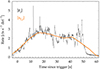 |
Fig. 1. Calculation of the variability. We show the 15–150-keV light curve {ri} of GRB 080319B as observed with BAT. The orange line shows the smoothed profile {sf, i} obtained with a smoothing timescale of Tf = 18.43 s, which collects a fraction f = 0.45 of the total fluence of the GRB. |
3.2. Estimate of the peak luminosity
Firstly, we used the estimates of Liso derived from broad-band modelling for all BAT GRBs, for which they were already available in the literature. For BAT GRBs with both KW and GBM estimates, we systematically preferred KW (Tsvetkova et al. 2017, 2021) after ensuring that they were consistent within the uncertainties. KW was preferred because it constrains the high-energy power-law index better, whereas GBM (NaI) is mainly limited by its smaller effective area above 100 keV (Tsvetkova et al. 2022). For the remaining BAT GRBs detected by KW, we adopted the same approach as in the KW catalogues: the isotropic luminosities were computed from the peak energy fluxes and k-corrected to the energy range 1/(1 + z) keV–10 MeV7. The peak spectrum was accumulated over a time interval Tp around the peak, which lasted longer than 64 ms so that enough photons could be collected. Under the assumption of negligible spectral evolution during Tp, we then rescaled the average flux resulted from fitting the spectrum by the ratio r64/rTp, where r64 and rTp are the peak count rate evaluated over 64 ms and the average count rate evaluated over Tp. Both count rates refer to the KW net counts in the ∼20–1200 keV light curves.
For the Fermi GRBs observed from the August 4, 2008, to June 20, 2018, we used the peak luminosity provided in the Fermi spectral catalogue (Poolakkil et al. 2021). For the remaining 40 more recent GBM bursts, the peak luminosity was computed as
 (2)
(2)
where dL is the luminosity distance, k is the k-correction and ϕp, 8 − 900 is the peak flux in the 8–900 keV energy range. The peak flux was computed from the best-fitting Band function of the spectrum accumulated over a 1.024 s window centred on the peak time and modelled with the GBM data tools. We ensured that our procedure yielded results consistent with those published in Poolakkil et al. (2021) with an accuracy of 30% by independently analysing a few common GRBs. For 22 of the 40 cases, we fixed it to the typical value of −2.3 because the high-energy spectral index of the Band function was poorly constrained (Preece et al. 2000; Kaneko et al. 2006; Guidorzi et al. 2011; Tsvetkova et al. 2017). The k-correction was obtained by renormalising the peak flux in the 1/(1 + z)–104/(1 + z) keV observer-frame energy band. For the final merged sample, we opted for the KW Liso estimate for each GRB in common between KW and GBM.
Lastly, for the long-duration merger candidate GRB 191019A (Levan et al. 2023), only BAT data were available. We extracted the 15–150 keV spectrum at peak centred at 0.272 s after the trigger time with an exposure of 0.128 s, as given by the detection timescale of MEPSA. Although a simple power-law yields an acceptable fit, the photon index of Γ = 1.78 ± 0.22 is suggestive of the presence of the peak energy of the νFν spectrum, Ep, within the BAT passband (Sakamoto et al. 2009). We therefore modelled it with the Band function (Band et al. 1993), fixing the low- and the high-energy indices to the typical values of −1 and −2.3, respectively. We found  keV. When we calculated the fluence in the 1 − 104 keV rest-frame band, the peak flux was (1.2 ± 0.2)×10−6 erg cm−2 s−1, corresponding to Liso = (2.6 ± 0.5)×1050 erg s−1.
4. Results
From the analysis of a common sample of BAT-GBM GRBs, for which significant measures of Vf were available for each of the three energy passbands (15–150, 8–150, and 150–900 keV), we found a weak dependence of Vf on the energy passband and on the used detector in most cases. In practice, taking the two sets of Vf estimates obtained from the full passbands of each detector (15–150 vs. 8–900 keV, respectively), which conveniently have the best S/N, 85–90% of them differ by ≲20%. Figure 2 shows the comparison between the two estimates of Vf for the specific case of f = 0.45 and β = 0.6. A more comprehensive comparison and analysis is reported in Appendix A.
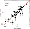 |
Fig. 2. Comparison between variability estimates obtained with BAT in the 15–150 keV band vs. the GBM estimates in the 8–900 keV band, obtained for a common sample and assuming f = 0.45 and β = 0.6. Equality is shown by the solid line. |
For the aim of this investigation, a ≲20% mismatch in Vf can be neglected, as shown by the dynamic range of Vf as well as the scatter observed in the Vf–L plane. Consequently, for the majority of GRBs we may neglect the dependence of Vf on the energy passbands, in agreement with what was found by R01.
For a common sample of 97 GRBs detected by Konus/WIND and Fermi/GBM, for which it was thus possible to independently estimate the 1–104 keV rest-frame Liso, we compared the two sets of values. The two sets are consistent overall over more than three decades. The distribution of the ratio Liso, KW/Liso, GBM presents a median value of 1.3 with [1.0, 1.6] as interquartile range8. The KW estimate is (30 ± 30)% higher because it can constrain the high-energy PL index better, as already discussed in Section 3.2. KW estimates are therefore preferable and were used for the sample of common GRBs. Overall, for the GRBs detected by GBM alone, a 30% discrepancy has a negligible impact on the Vf–L correlation, as we show below.
4.1. Variability versus peak luminosity
It was originally found by R01 that the most significant correlation between Vf and Liso is obtained for f = 0.45. β was fixed to 0.6 because of the contrasting effects of cosmic dilation, which would demand β = 1, and of the narrowing of pulses with energy, which would instead imply β = −0.4 (see R01).
In the evaluation of the statistical significance of the Vf–Liso correlation that follows, we first of all ignored the four long-duration merger candidates, and we show them only for comparison at the end.
We systematically calculated the correlation coefficients (Pearson r, Spearman ρ, and Kendall τ) between log Vf and log Liso for the entire grid of (f, β) values (Section 3). We explored β ≠ 0.6 values for the sake of completeness. For any values of (f, β) we considered only the pairs (Vf, Liso) with a Vf > 0 at 90% confidence; the remaining GRBs were simply ignored because their 90% upper limits on Vf did not turn out to be usefully constraining in the Vf–Liso plane. Consequently, the number of selected GRBs varies for different (f, β) values. Overall, the joint sample includes 216 GRBs with significant estimates for both observables: hereafter, this is referred to as the merged sample.
We first restricted ourselves to the β = 0.6 cases for the reasons explained above. The highest degree of correlation using Pearson’s r coefficient is found for f = 0.8 from a sample of 212 GRBs: the p-values associated with r, ρ, and τ are 3.1 × 10⁻⁴, 4.9 × 10⁻³, and 5.7 × 10⁻³, respectively. The result is shown in Figure 3, whose values are reported in Table 1. Alternatively, using non-parametric ρ and τ, the most significant case is obtained for f = 0.9 and 215 GRBs, with p-values that are comparable with the f = 0.8 case: 8.5 × 10⁻⁴, 4.0 × 10⁻³, and 3.9 × 10⁻³ for r, ρ, and τ, respectively. Consequently, we may consider the f = 0.8 and f = 0.9 statistically equivalent in essence.
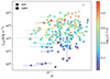 |
Fig. 3. Variability–luminosity correlation obtained for f = 0.8 and β = 0.6. This value of f gives the highest degrees of correlation. Different symbols refer to the different detectors used to measure Vf. For BAT-GBM shared GRBs, we used BAT values. Pentagons represent long-duration merger candidates. The redshift information is also available through the colour-coded scale. |
When we relaxed the constraint β = 0.6, the improvement in the correlation was rather small: the lowest p-value for r decreases to 1.6 × 10⁻⁴ obtained for (f = 0.75, β = 1.0), whereas the lowest p-values of ρ and τ become 2.2 × 10⁻³ for (f = 0.9, β = 0.4). Therefore, admitting the possibility that β differs from the physically grounded value of 0.6 does not significantly improve the degree of correlation between Vf and Liso. Consequently, hereafter we limit the discussion to the β = 0.6 case. Table 2 reports the correlation coefficients and p-values for all values of f, along with the number of GRBs with significant measures that were considered in each case.
Correlation coefficients of the Vf–Liso relation for the joint BAT-GBM sample, assuming β = 0.6.
The selection of f = 0.8 (or f = 0.9) as the best-correlation case is the result of a multi-trial process, where the optimal value was selected out of 17 trial values for f in the range 0.1–0.9. On the one hand, these are not completely independent because they are due to different ways of processing the same LCs. On the other hand, they are still the results of an optimal selection from multiple attempts.
To determine the effective p-value, that is, the probability that the observed degree of correlation is compatible with null hypothesis of no correlation, we carried out 104 simulations, each of which consisted of shuffling the array of peak luminosities and determining the best-correlation case for each synthetic sample of (Vf, Liso) pairs in the very same way as we did for the real sample. p-values equal to or lower than the corresponding lowest real values of (r, ρ, τ) were obtained in 26, 251, and 232 cases: the effective p-values therefore are 2.6 × 10⁻³, 2.5%, and 2.3%, respectively. We conclude that the effective probability to obtain by accident an equally or more correlated sample in Vf–Liso space than what was shown in Fig. 3, under the null hypothesis of no correlation, is ≲2%, which is equivalent to the range 2.2–3.0σ (Gaussian).
4.2. Comparison with previous results
To compare the results with what was previously obtained by G05, we had to the use the values obtained for f = 0.45, which was considered at the time. The resulting Vf–Liso distribution is shown in Figure 4. Using this value for f, the sample of significant pairs (Vf, Liso) decreases to 184 and the p-values of the linear and non-parametric correlation tests increase to 3.6% and 25%, respectively, so that the previously found and very marginal evidence for a correlation essentially vanishes. Table 3 reports all the values of Vf and Liso for this sample.
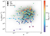 |
Fig. 4. Variability–luminosity correlation obtained for f = 0.45 and β = 0.6. In addition to the 184 GRBs analysed in the present work, we also show (stars) GRBs from G05. The redshift is colour-coded. The shaded region shows a density map, obtained using a kernel density estimate, of the same data set (excluding the G05 GRBs). The four GRBs with red pentagons are long-duration merger candidates (GRB 060614, GRB 191019A, GRB 211211A, and GRB 230307A) that were considered separately. |
G05 considered 32 GRBs: ignoring GRB 980425, which is a peculiar low-luminosity event (Kulkarni et al. 1998; Li & Chevalier 1999; Pian et al. 2000; Soderberg et al. 2004; Ghisellini et al. 2006), GRB 050603 whose redshift was later questioned (Hjorth et al. 2012), and another 5 Swift/BAT GRBs that are already included in the present sample, we are left with 25 additional GRBs from G05, adding which, we end up with a sample of 209 GRBs whose p-values are 4.7 × 10⁻³ (Pearson) and 3.8 and 4.1% for the other non-parametric tests. The luminosity values in G05 were calculated in the 100−1000 keV band, as originally done by R01. We then replaced their luminosity values with the broadband 1 − 104 keV rest-frame analogues as reported in the literature as derived from broad-band spectroscopy. Compared with the G05 values, the luminosities in most cases increased by a factor between 2 and 3.
In Appendix B we estimate a ≳3% probability that the correlation assessed in G05 was accidental and caused by the poor sampling of the variability-luminosity space. In addition, it is also possible that different selection effects between the joint sample of BAT-GBM of the present work and the early one of G05 also play a role: in particular, both GRB samples inevitably depend on the different suites of prompt optical follow-up facilities that enabled the afterglow identification and secured the redshift measurement.
4.3. Relation with the number of peaks
Figure 5 is the same as Figure 4, except for the colours, which display the number of peaks of each GRB, Npeaks, as determined by us in Guidorzi et al. (2024) and in Maccary et al. (2024b) using MEPSA (Guidorzi 2015) and selecting peaks with S/N > 5.
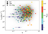 |
Fig. 5. Same plot as Figure 4, except for the colour-code, which corresponds to five different classes of number of peaks. |
The additional information supplied by Npeaks helped us to characterise the GRBs with low Vf that were mostly missing in the early sample of G05 and which contributed to demoting the correlation. Most GRBs with Vf < 0.05 have very few peaks (mainly one or two) and are 25% of the whole sample. On average, these low-Vf GRBs exhibit comparable luminosities with the complementary sample of more variable GRBs, except for some with Liso ≲ 1050 erg s−1. Figure 6 displays the LCs of five low-Vf GRBs, along with G05 GRB 0002109. All of them have Vf ≲ 0.03, which is in line with a relatively smooth profile, and Liso in the range 1052–1054 erg s−1. Except for some modulation in GRB 150314A, their profiles look like smooth, fast-rise exponential-decay (FRED) pulses. In principle, an external origin for their prompt emission cannot be excluded (a thorough analysis of how tenable this scenario is for each of them, taking into account the corresponding afterglow multi-band data sets, is beyond the scope of the present work). Specifically, in the case of GRB 200829A, an external origin has been put forward (Li et al. 2023), whereas Samuelsson et al. (2022) discussed a photospheric origin for GRB 150314A.
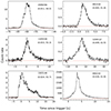 |
Fig. 6. Collection of six observer-frame GRBs with medium to high luminosity and low variability. Each panel reports the GRB name along with the (Vf, log Liso) pair. All of them are BAT bursts (15–150 keV), except for BeppoSAX GRB 000210 (40–700 keV) in the bottom right panel. In the case of BAT LCs, the count rates are expressed in count s−1 per fully illuminated detector for an equivalent on-axis source. |
4.4. Long-duration merger candidates
The GRBs detected by either BAT or GBM contain at least four credible long-duration merger candidates known to date: GRB 060614 (Della Valle et al. 2006; Fynbo et al. 2006), GRB 191019A (Levan et al. 2023), GRB 211211A (Yang et al. 2022; Troja et al. 2022), and GRB 230307A (Levan et al. 2024). GRB 060505 (Fynbo et al. 2006) should also be considered, but we ignored it because of the low S/N of BAT data along with its controversial nature (McBreen et al. 2008). Although they were not included in the samples for the statistical analysis of the Vf–Liso correlation, we added them in Figures 4 and 5.
Two of them (GRB 060614 and GRB 191019A) lie within a region of their own: Vf > 0.1 and Liso < 1051 erg s−1. GRB 211211A has a comparable Vf, but higher Liso (2 × 1051 erg s−1), still lying in the outskirts of the distribution of standard long GRBs. Only GRB 230307A lies within a more densely populated region. All of them feature many peaks (ranging from 14 to 54), which contributed to the high values of Vf. Three out of four known candidates lie off the population distribution in the Vf–Liso plane. This suggests that the unusual combination of Vf ≳ 0.1 and Liso ≲ 1051 erg s−1 might be a good indicator for a merger origin. In this respect, a possible closely related indicator was already tentatively identified in the MVT (Camisasca et al. 2023a,b; Veres et al. 2023).
To determine whether there are other similar and as-yet disguised merger candidates, we explored the LC morphology of the GRBs that lie mostly in the high-Vf/low Liso. Figure 7 displays a collection of ten such GRBs, all of which share the following properties: Vf > 0.1 and Liso ≲ 1052 erg s−1 s, with the only exception of 190719C (Liso = 3 × 1052 erg s−1), which has the highest Vf of all GRBs and whose projected offset seems to be more typical of a merger event and rather large for a collapsar event, although not unprecedented (Rossi et al. 2019). These ten GRBs include some whose collapsar identity was firmly established by evidence for an associated SN: GRB 091127 (Cobb et al. 2010; Berger et al. 2011) and GRB 111228A (Klose et al. 2019). Some interesting events look like short GRB with extended emission, such as GRB 161129A, as was also noted by the Swift team. Its nature remained inconclusive, however, given the spectral softness of the initial spike in comparison with the bulk population of short GRBs with and without extended emission (Barthelmy et al. 2016).
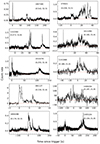 |
Fig. 7. Collection of ten observer-frame GRBs with high variability, Vf > 0.1, and relatively low luminosity, Liso ≲ 1052 erg s−1. Each panel reports the GRB name along with the (Vf, log Liso) pair. All of them are BAT bursts (15–150 keV), except for Fermi GRB 140623A (8–900 keV). In the case of BAT LCs, the count rates are expressed in count s−1 per fully illuminated detector for an equivalent on-axis source. |
4.5. Variability and minimum variability timescale
Given that GRB time variability is a recurring general property that is often called for and interpreted in the literature, it is worth investigating and clarifying the relation between the definition of the variability Vf considered in this work and the concept of the MVT. To better illustrate this point, Figure 8 shows the two quantities calculated for a subsample of 184 GRBs. The MVT values were either taken from or calculated as in Camisasca et al. (2023a).
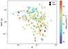 |
Fig. 8. MVT vs. variability for a subsample of 184 GRBs. The pentagons show the four long-duration merger candidates. The MVT values were calculated as in Camisasca et al. (2023a). Liso is colour-coded. |
The two quantities are clearly neither independent nor tightly correlated. The MVT identifies the shortest timescale over which a significant and uncorrelated flux variation is observed, regardless of the overall properties of the whole LC, whereas Vf quantifies how much variance lies at short timescales with respect to long ones, where the separation into short and long is dictated by the net time interval over which a sizeable fraction of energy is released (Section 3.1).
It is therefore no wonder that for Vf ≳ 0.1 all possible MVT values from 0.01 to ∼30 s are observed: a high value of Vf does not necessarily imply the presence of narrow pulses, but it could also be obtained for a GRB featuring several broad peaks with different timescales and interspersed with quiescent times. Instead, most GRBs with Vf ≲ few × 10−2 inevitably miss narrow spikes, such that their MVT is ≳a few seconds.
5. Discussion
Variable GRBs are expected to arise when internal dissipation processes (e.g. internal shocks) occur outside the e± pair photosphere, while X-ray rich bursts may arise from the processes occurring below it (Kobayashi et al. 2002; Mészáros et al. 2002). Let d and D be the width and separation of the random shells that characterise a GRB jet with an irregular velocity. The hydrodynamic timescale d/c and the angular spreading timescale D/c determine the rise and decay time of a gamma-ray pulse, respectively. Since most observed pulses rise more quickly than they decay, the pulse width and pulse separation are mainly determined by the angular spreading time D/c (Norris et al. 1996; Ryde & Petrosian 2002).
The distribution of peak separations10 {D/c} for a GRB light curve usually has a large dispersion (Nakar & Piran 2002; Guidorzi et al. 2015). While the fastest variability timescale in a GRB can be as short as a few dozen milliseconds (Camisasca et al. 2023a), the largest peak separation or the total duration is usually much longer. Since shell collisions producing narrow pulses typically occur at small radii ∼DΓ2, the photosphere might obscure them and might primarily leave the wider pulses visible. This causes the temporal profile to be smooth. When a jet has a smaller typical Lorentz factor, a larger fraction of the collisions occurs at small radii ∼DΓ2 below the photosphere. The smoothing effect is therefore expected to be stronger.
The observed correlation between luminosity and variability in GRBs has been interpreted as reflecting a relation between the GRB jet opening angle and the mass involved in the explosion (Kobayashi et al. 2002). Since the beaming-corrected gamma-ray energy was thought to be narrowly clustered in the pre-Swift era, narrower jets would emit brighter gamma-ray emission. If narrower jets have typically higher Lorentz factors due to lower mass loading, the photosphere could induce the luminosity and variability correlation. For the increased number of GRBs that were observed in the Swift era, it was found that the distribution of beaming-corrected gamma-ray energy is broader than previously thought, although still narrower than the distribution of isotropic energy (Liang et al. 2008).
The correlation between luminosity and variability is not significant for our larger sample of GRBs. To investigate potential indications of the photospheric effect in the GRB light curves, we tested for a correlation between Lorentz factors and variability Vf, as slower jets might induce a stronger photospheric smoothing effect. However, we again find no significant correlations for the 37 GRBs whose Lorentz factors were estimated from the afterglow onset times tp (Ghirlanda et al. 2018). The p-values associated with linear and non-parametric correlation coefficients are 4 and 24%, respectively. This contrasts with the MVT, which shows a negative correlation with the Lorentz factor, albeit with significant scatter: MVT ∝ Γ−2 (see Fig. 13 of Camisasca et al. 2023a). This relation is consistent with the photospheric model in which the MVT is determined by the curvature timescale at the photoshere: MVT ∼ R±/cΓ2, although the radii estimated from the MVT and Γ are rather large, 1015 − 17 cm, for the photospheric radii R± (Camisasca et al. 2023a; Kobayashi et al. 2002).
As shown in Fig. 8 and discussed in Section 4.5, the correlation between the MVT and the variability Vf is very weak. The average power density spectrum (PDS) of very long GRBs (with T90 > 100 s) is known to follow a power-law distribution characterised by a slope α ∼ −5/3, featuring a clear break at about 1 Hz (Beloborodov et al. 2000; Guidorzi et al. 2012; Dichiara et al. 2013). Shorter GRBs exhibit PDS slopes that are more significantly influenced by statistical fluctuations. The lack of a correlation between the MVT and the variability Vf can be attributed to the dominance of significant components in the light curve power spectrum at timescales that are substantially longer than the MVT (i.e. Vf is also determined by the pulses with longer timescales and by quiescent times). Considering that the MVT is better correlated with Liso and Γ, it is likely to be more sensitive to the photospheric cut-off of the variability timescales; or, intrinsically the absolute measure of the short timescale with significant variance is correlated with them. If the MVT is set by the photospheric effect, then the 1 Hz break in the averaged PDS should be due to the intrinsic nature of the central engine activity (i.e. the intrinsic separation distribution {D}).
A possible factor that weakens the correlation between Lorentz factors and variability Vf can be the separation distribution {D}, which can intrinsically vary significantly between events. Even when the average PDS follows the power law, especially for events with only a few peaks, the statistical fluctuations can be significant. When some events intrinsically lack narrowest components or when longer-timescale components in the power spectrum dominate, their variability would be insensitive to the Lorentz factor of the jet and is always low. Another potential weakening factor is the errors in the estimates of Lorentz factors. Numerous collisions occur during an evolution of multiple shells. Each collision produces a pulse. However, the main pulses are produced by collisions between the fastest shells, ∼Γmax, and the slowest shells, ∼Γmin. A collision like this occurs at R ∼ Γmin2Di for an initial separation Di. The suppression of narrow peaks and consequent smoothing effect basically depend on the extent to which the photosphere radius R± is larger than Γmin2 Dmin. The Lorentz factor based on the afterglow onset time gives a characteristic value after the internal dissipation process is settled, but it might not correlate well with the minimum value Γmin of the intrinsic distribution.
In addition, it is also possible that GRBs whose prompt emission had a completely different origin contributed to weaken the possible correlation between Vf and Liso. Specifically, this might be the case of low-Vf GRBs, which show just one broad peak and a typical Liso. Their prompt emission might have an external origin, marking the high-energy afterglow onset (Section 4.3 and Fig. 5). For five of the six external-shock GRB candidates shown in Fig. 6, upper limits of the afterglow onset time tp are available (see Table 4). We find tight upper limits especially for four of these events. The afterglow might onset immediately after or during the prompt gamma-ray emission, or the prompt gamma-ray emission itself could be the afterglow onset as we propose the external shock origin. Interestingly, two of these events (GRB 091018 and GRB 120811C) have very low Ep. Taking the Ep distribution of the merged sample of 317 GRBs from Tsvetkova et al. (2017, 2021), only one object (∼0.3%) and 33 objects (10%) have equal or smaller Ep than these two bursts, respectively.
Finally, in Section 4.4 and in Figure 4 we showed that three out of four known long-duration compact binary merger candidates lie off the bulk of long GRBs, in the region with Vf > 0.1 and Liso < 1051 erg s−1, and the fourth, GRB 230307A, lies closer to other typical long GRBs. Additionally, considering their MVT (Fig. 8 and Camisasca et al. 2023a), these events appear to be characterised by the rare combination of a very small MVT (a few dozen milliseconds), high variability, and relatively low luminosity. We tentatively identified other interesting events that are displayed in Fig. 7 and have analogous features. Although for some them, an associated SN was found, the remaining candidates might be worth a deeper investigation.
6. Conclusions
Twenty years after the launch of Swift and its subsequent enhancement by Fermi, the number of GRBs with measured redshifts has significantly increased. This growth necessitates a new more statistically robust examination of the variability-luminosity relation. This relation was previously reported based on a sample of approximately 30 GRBs that were available a few years after the initial afterglow discoveries.
The aim of this study was to test the correlation by using the extensive data sets available today. Based on a sample of 216 GRBs detected by Swift, Fermi, and Konus/WIND, each with robust estimates for the variability Vf and the isotropic-equivalent peak luminosity Liso, we found that the scatter has increased to such an extent that the correlation can no longer be considered statistically significant (p-value ≲ 2%).
The definition of Vf adopted in this study, originally provided by R01, measures the temporal power of short to intermediate timescales with respect to the total power, which includes the contribution from all timescales. This definition of Vf is not be confused with that of the MVT (MacLachlan et al. 2013; Golkhou & Butler 2014; Golkhou et al. 2015; Camisasca et al. 2023a), which is another observable that is used to characterise GRB variability. The MVT corresponds to the shortest timescale over which a statistically significant and uncorrelated flux change is observed, regardless of the power on long timescales. Here, we investigated the relation between Vf and MVT for the first time and found a weak correlation (Fig. 8). This finding helps to explain why the MVT is found to be anti-correlated with Liso and the Lorentz factor Γ (measured from the afterglow onset time), despite significant scatter (Camisasca et al. 2023a), while Vf does not.
When internal dissipation occurs within the e± photosphere, the resulting gamma-ray light curve is smoothed out. Narrower pulses, produced at smaller radii, are particularly sensitive to this photospheric cut-off. The stronger correlation of Liso and Γ with the MVT compared to Vf suggests that Vf is mainly influenced by pulses and quiescent periods with timescales much longer than the MVT scale. The MVT might be determined by the photospheric effect or is intrinsically correlated with Liso and Γ due to the unknown nature of the central engine.
Furthermore, we identified several GRBs with a single broad and smooth peak, low Vf, and typical Liso, whose origin may be attributed to external shocks. In this, they differ from the majority of the observed GRBs (Fig. 6). This scenario is supported by the tight upper limits on the afterglow onset times determined from early optical afterglow observations. Notably, the prompt emissions of two of them (GRB 091018 and GRB 120811C) are very soft, having peak energies of the time-average ν Fν spectrum in the low tail of the observed population.
Lastly, the combination of high variability (Vf > 0.1), relatively low luminosity (Liso < 1051 erg s−1), and short MVT (≲0.1 s; Camisasca et al. 2023a) appears to be a promising indicator for a compact binary merger origin, despite the long duration and deceptive time profile. We have tentatively identified other potential candidates with similar characteristics.
Data availability
Tables 1 and 3 are available at the CDS via anonymous ftp to cdsarc.cds.unistra.fr (130.79.128.5) or via https://cdsarc.cds.unistra.fr/viz-bin/cat/J/A+A/690/A261
An alternative interpretation as a disguised tidal disruption event was also put forward for this event (Eyles-Ferris et al. 2024).
We made an exception for 191019A, given the interest in this merger candidate along with the possibility of constraining the peak energy.
This ensured that long-lasting weak but statistically significant tails were not cut off.
As explained in Tsvetkova et al. (2017, 2021), using the rest-frame upper boundary of 10 (1 + z) MeV instead of 10 MeV compensates for the fact that the Konus/WIND energy range extends to 10–25 MeV.
This range comprises the two central quartiles, that is, the 25–75 percentiles.
This BeppoSAX gamma-ray luminous and optically dark GRB was discussed in detail in Piro et al. (2002).
Also known as waiting times.
We used the scipy.stats.binomtest function.
The function ks2d2s from Press et al. (1992) was used.
Acknowledgments
D.F., A.L., A.R., D.S., M.U. acknowledge financial support from the basic funding program of the Ioffe Institute FFUG-2024-0002. A.T. acknowledges financial support from “ASI-INAF Accordo Attuativo HERMES Pathinder operazioni n. 2022-25-HH.0” (discussion of the results, editing the paper) and the basic funding program of the Ioffe Institute FFUG-2024-0002 (computation of Liso). L.F. acknowledges support from the AHEAD-2020 Project grant agreement 871158 of the European Union’s Horizon 2020 Program. We thank the reviewer for their detailed and constructive report.
References
- Abbott, B. P., Abbott, R., Abbott, T. D., et al. 2017, ApJ, 848, L13 [CrossRef] [Google Scholar]
- Band, D., Matteson, J., Ford, L., et al. 1993, ApJ, 413, 281 [Google Scholar]
- Barthelmy, S. D., Cummings, J. R., Gehrels, N., et al. 2016, GRB Coordinates Network, 20220, 1 [NASA ADS] [Google Scholar]
- Beloborodov, A. M., Stern, B. E., & Svensson, R. 2000, ApJ, 535, 158 [NASA ADS] [CrossRef] [Google Scholar]
- Berger, E., Chornock, R., Holmes, T. R., et al. 2011, ApJ, 743, 204 [CrossRef] [Google Scholar]
- Blinnikov, S. I., Novikov, I. D., Perevodchikova, T. V., & Polnarev, A. G. 1984, Sov. Astron. Lett., 10, 177 [Google Scholar]
- Camisasca, A. E., Guidorzi, C., Amati, L., et al. 2023a, A&A, 671, A112 [NASA ADS] [CrossRef] [EDP Sciences] [Google Scholar]
- Camisasca, A. E., Guidorzi, C., Bulla, M., et al. 2023b, GRB Coordinates Network, 33577, 1 [NASA ADS] [Google Scholar]
- Cobb, B. E., Bloom, J. S., Perley, D. A., et al. 2010, ApJ, 718, L150 [NASA ADS] [CrossRef] [Google Scholar]
- Della Valle, M., Chincarini, G., Panagia, N., et al. 2006, Nature, 444, 1050 [NASA ADS] [CrossRef] [Google Scholar]
- Dichiara, S., Guidorzi, C., Amati, L., & Frontera, F. 2013, MNRAS, 431, 3608 [NASA ADS] [CrossRef] [Google Scholar]
- Dichiara, S., Tsang, D., Troja, E., et al. 2023, ApJ, 954, L29 [NASA ADS] [CrossRef] [Google Scholar]
- Eichler, D., Livio, M., Piran, T., & Schramm, D. N. 1989, Nature, 340, 126 [NASA ADS] [CrossRef] [Google Scholar]
- Eyles-Ferris, R. A. J., Nixon, C. J., Coughlin, E. R., & O’Brien, P. T. 2024, ApJ, 965, L20 [NASA ADS] [CrossRef] [Google Scholar]
- Fenimore, E. E., Ramirez-Ruiz, E., & Wu, B. 1999, ApJ, 518, L73 [NASA ADS] [CrossRef] [Google Scholar]
- Fenimore, E. E., & Ramirez-Ruiz, E. 2000, ArXiv e-prints [arXiv:astro-ph/0004176] [Google Scholar]
- Frederiks, D., Golenetskii, S., Aptekar, R., et al. 2016, GRB Coordinates Network, 20059, 1 [NASA ADS] [Google Scholar]
- Frederiks, D., Golenetskii, S., Aptekar, R., et al. 2017, GRB Coordinates Network, 20995, 1 [NASA ADS] [Google Scholar]
- Frederiks, D., Golenetskii, S., Aptekar, R., et al. 2018a, GRB Coordinates Network, 22546, 1 [NASA ADS] [Google Scholar]
- Frederiks, D., Golenetskii, S., Aptekar, R., et al. 2018b, GRB Coordinates Network, 23011, 1 [Google Scholar]
- Frederiks, D., Golenetskii, S., Aptekar, R., et al. 2018c, GRB Coordinates Network, 23061, 1 [NASA ADS] [Google Scholar]
- Frederiks, D., Golenetskii, S., Aptekar, R., et al. 2019, GRB Coordinates Network, 26576, 1 [NASA ADS] [Google Scholar]
- Frederiks, D., Golenetskii, S., Aptekar, R., et al. 2020, GRB Coordinates Network, 29084, 1 [NASA ADS] [Google Scholar]
- Frederiks, D., Golenetskii, S., Lysenko, A., et al. 2021a, GRB Coordinates Network, 30196, 1 [NASA ADS] [Google Scholar]
- Frederiks, D., Golenetskii, S., Lysenko, A., et al. 2021b, GRB Coordinates Network, 30366, 1 [NASA ADS] [Google Scholar]
- Frederiks, D., Golenetskii, S., Lysenko, A., et al. 2021c, GRB Coordinates Network, 30694, 1 [NASA ADS] [Google Scholar]
- Frederiks, D., Lysenko, A., Ridnaia, A., et al. 2023a, GRB Coordinates Network, 34511, 1 [NASA ADS] [Google Scholar]
- Frederiks, D., Lysenko, A., Ridnaia, A., et al. 2023b, GRB Coordinates Network, 35377, 1 [NASA ADS] [Google Scholar]
- Frederiks, D., Lysenko, A., Ridnaia, A., et al. 2024, GRB Coordinates Network, 35701, 1 [NASA ADS] [Google Scholar]
- Fynbo, J. P. U., Watson, D., Thöne, C. C., et al. 2006, Nature, 444, 1047 [NASA ADS] [CrossRef] [Google Scholar]
- Gehrels, N., Chincarini, G., Giommi, P., et al. 2004, ApJ, 611, 1005 [Google Scholar]
- Gehrels, N., Norris, J. P., Barthelmy, S. D., et al. 2006, Nature, 444, 1044 [NASA ADS] [CrossRef] [Google Scholar]
- Ghirlanda, G., Nappo, F., Ghisellini, G., et al. 2018, A&A, 609, A112 [NASA ADS] [CrossRef] [EDP Sciences] [Google Scholar]
- Ghisellini, G., Ghirlanda, G., Mereghetti, S., et al. 2006, MNRAS, 372, 1699 [NASA ADS] [CrossRef] [Google Scholar]
- Goldstein, A., Cleveland, W. H., & Kocevski, D. 2022, Fermi GBM Data Tools: V1.1.1, https://fermi.gsfc.nasa.gov/ssc/data/analysis/gbm [Google Scholar]
- Golkhou, V. Z., & Butler, N. R. 2014, ApJ, 787, 90 [NASA ADS] [CrossRef] [Google Scholar]
- Golkhou, V. Z., Butler, N. R., & Littlejohns, O. M. 2015, ApJ, 811, 93 [NASA ADS] [CrossRef] [Google Scholar]
- Gompertz, B. P., Ravasio, M. E., Nicholl, M., et al. 2023, Nat. Astron., 7, 67 [Google Scholar]
- Guidorzi, C. 2015, Astron. Comput., 10, 54 [NASA ADS] [CrossRef] [Google Scholar]
- Guidorzi, C., Frontera, F., Montanari, E., et al. 2005, MNRAS, 363, 315 [NASA ADS] [CrossRef] [Google Scholar]
- Guidorzi, C., Frontera, F., Montanari, E., et al. 2006, MNRAS, 371, 843 [NASA ADS] [CrossRef] [Google Scholar]
- Guidorzi, C., Lacapra, M., Frontera, F., et al. 2011, A&A, 526, A49 [NASA ADS] [CrossRef] [EDP Sciences] [Google Scholar]
- Guidorzi, C., Margutti, R., Amati, L., et al. 2012, MNRAS, 422, 1785 [NASA ADS] [CrossRef] [Google Scholar]
- Guidorzi, C., Dichiara, S., Frontera, F., et al. 2015, ApJ, 801, 57 [NASA ADS] [CrossRef] [Google Scholar]
- Guidorzi, C., Sartori, M., Maccary, R., et al. 2024, A&A, 685, A34 [NASA ADS] [CrossRef] [EDP Sciences] [Google Scholar]
- Hjorth, J., Malesani, D., Jakobsson, P., et al. 2012, ApJ, 756, 187 [Google Scholar]
- Kaneko, Y., Preece, R. D., Briggs, M. S., et al. 2006, ApJS, 166, 298 [CrossRef] [Google Scholar]
- Kimura, S. S. 2023, in The Encyclopedia of Cosmology. Set 2: Frontiers in Cosmology. Volume 2: Neutrino Physics and Astrophysics, ed. F. W. Stecker, 433 [CrossRef] [Google Scholar]
- Klose, S., Schmidl, S., Kann, D. A., et al. 2019, A&A, 622, A138 [NASA ADS] [CrossRef] [EDP Sciences] [Google Scholar]
- Kobayashi, S., Ryde, F., & MacFadyen, A. 2002, ApJ, 577, 302 [NASA ADS] [CrossRef] [Google Scholar]
- Kulkarni, S. R., Frail, D. A., Wieringa, M. H., et al. 1998, Nature, 395, 663 [NASA ADS] [CrossRef] [Google Scholar]
- Lesage, S., Veres, P., Briggs, M. S., et al. 2023, ApJ, 952, L42 [NASA ADS] [CrossRef] [Google Scholar]
- Levan, A. J., Malesani, D. B., Gompertz, B. P., et al. 2023, Nat. Astron., 7, 976 [NASA ADS] [CrossRef] [Google Scholar]
- Levan, A. J., Gompertz, B. P., Salafia, O. S., et al. 2024, Nature, 626, 737 [NASA ADS] [CrossRef] [Google Scholar]
- Li, Z.-Y., & Chevalier, R. A. 1999, ApJ, 526, 716 [NASA ADS] [CrossRef] [Google Scholar]
- Li, J., Lin, D.-B., Lu, R.-J., et al. 2023, ApJ, 944, 21 [NASA ADS] [CrossRef] [Google Scholar]
- Liang, E.-W., Racusin, J. L., Zhang, B., Zhang, B.-B., & Burrows, D. N. 2008, ApJ, 675, 528 [NASA ADS] [CrossRef] [Google Scholar]
- Lien, A., Sakamoto, T., Barthelmy, S. D., et al. 2016, ApJ, 829, 7 [Google Scholar]
- Maccary, R., Guidorzi, C., Amati, L., et al. 2024a, ApJ, 965, 72 [NASA ADS] [CrossRef] [Google Scholar]
- Maccary, R., Maistrello, M., Guidorzi, C., et al. 2024b, A&A, 688, L8 [NASA ADS] [CrossRef] [EDP Sciences] [Google Scholar]
- MacFadyen, A. I., & Woosley, S. E. 1999, ApJ, 524, 262 [NASA ADS] [CrossRef] [Google Scholar]
- MacLachlan, G. A., Shenoy, A., Sonbas, E., et al. 2012, MNRAS, 425, L32 [NASA ADS] [CrossRef] [Google Scholar]
- MacLachlan, G. A., Shenoy, A., Sonbas, E., et al. 2013, MNRAS, 432, 857 [NASA ADS] [CrossRef] [Google Scholar]
- McBreen, S., Foley, S., Watson, D., et al. 2008, ApJ, 677, L85 [NASA ADS] [CrossRef] [Google Scholar]
- Mészáros, P. 2017, in Neutrino Astronomy: Current Status, Future Prospects, eds. T. Gaisser, & A. Karle, 1 [Google Scholar]
- Mészáros, P., Ramirez-Ruiz, E., Rees, M. J., & Zhang, B. 2002, ApJ, 578, 812 [Google Scholar]
- Murase, K., & Bartos, I. 2019, Annu. Rev. Nucl. Part. Sci., 69, 477 [NASA ADS] [CrossRef] [Google Scholar]
- Nakar, E., & Piran, T. 2002, MNRAS, 331, 40 [NASA ADS] [CrossRef] [Google Scholar]
- Narayan, R., Paczynski, B., & Piran, T. 1992, ApJ, 395, L83 [NASA ADS] [CrossRef] [Google Scholar]
- Nava, L. 2021, Universe, 7, 503 [NASA ADS] [CrossRef] [Google Scholar]
- Noda, K., & Parsons, R. D. 2022, Galaxies, 10, 7 [NASA ADS] [CrossRef] [Google Scholar]
- Norris, J. P., & Bonnell, J. T. 2006, ApJ, 643, 266 [NASA ADS] [CrossRef] [Google Scholar]
- Norris, J. P., Nemiroff, R. J., Bonnell, J. T., et al. 1996, ApJ, 459, 393 [NASA ADS] [CrossRef] [Google Scholar]
- Paczynski, B. 1991, Acta Astron., 41, 257 [NASA ADS] [Google Scholar]
- Paczyński, B. 1998, ApJ, 494, L45 [Google Scholar]
- Pian, E., Amati, L., Antonelli, L. A., et al. 2000, ApJ, 536, 778 [Google Scholar]
- Piro, L., Frail, D. A., Gorosabel, J., et al. 2002, ApJ, 577, 680 [NASA ADS] [CrossRef] [Google Scholar]
- Planck Collaboration VI. 2020, A&A, 641, A6 [NASA ADS] [CrossRef] [EDP Sciences] [Google Scholar]
- Poolakkil, S., Preece, R., Fletcher, C., et al. 2021, ApJ, 913, 60 [NASA ADS] [CrossRef] [Google Scholar]
- Preece, R. D., Briggs, M. S., Mallozzi, R. S., et al. 2000, ApJS, 126, 19 [Google Scholar]
- Preece, R., Burgess, J. M., von Kienlin, A., et al. 2014, Science, 343, 51 [Google Scholar]
- Press, W. H., Teukolsky, S. A., Vetterling, W. T., & Flannery, B. P. 1992, Numerical Recipes in C. The Art of Scientific Computing (Cambridge: Cambridge University Press) [Google Scholar]
- Racusin, J. L., Karpov, S. V., Sokolowski, M., et al. 2008, Nature, 455, 183 [Google Scholar]
- Reichart, D. E., Lamb, D. Q., Fenimore, E. E., et al. 2001, ApJ, 552, 57 [Google Scholar]
- Ridnaia, A., Golenetskii, S., Aptekar, R., et al. 2020, GRB Coordinates Network, 28323, 1 [NASA ADS] [Google Scholar]
- Rossi, A., Heintz, K. E., Fynbo, J. P. U., et al. 2019, GRB Coordinates Network, 25252, 1 [NASA ADS] [Google Scholar]
- Ryde, F., & Petrosian, V. 2002, ApJ, 578, 290 [NASA ADS] [CrossRef] [Google Scholar]
- Sakamoto, T., Sato, G., Barbier, L., et al. 2009, ApJ, 693, 922 [NASA ADS] [CrossRef] [Google Scholar]
- Samuelsson, F., Lundman, C., & Ryde, F. 2022, ApJ, 925, 65 [NASA ADS] [CrossRef] [Google Scholar]
- Soderberg, A. M., Kulkarni, S. R., Berger, E., et al. 2004, Nature, 430, 648 [NASA ADS] [CrossRef] [Google Scholar]
- Sonbas, E., MacLachlan, G. A., Dhuga, K. S., et al. 2015, ApJ, 805, 86 [NASA ADS] [CrossRef] [Google Scholar]
- Sun, H., Wang, C. W., Yang, J., et al. 2023, ArXiv e-prints [arXiv:2307.05689] [Google Scholar]
- Svinkin, D., Golenetskii, S., Aptekar, R., et al. 2016, GRB Coordinates Network, 20197, 1 [NASA ADS] [Google Scholar]
- Svinkin, D., Golenetskii, S., Aptekar, R., et al. 2018, GRB Coordinates Network, 22825, 1 [NASA ADS] [Google Scholar]
- Svinkin, D., Golenetskii, S., Aptekar, R., et al. 2019, GRB Coordinates Network, 24015, 1 [NASA ADS] [Google Scholar]
- Svinkin, D., Golenetskii, S., Frederiks, D., et al. 2021, GRB Coordinates Network, 30276, 1 [NASA ADS] [Google Scholar]
- Svinkin, D., Frederiks, D., Lysenko, A., et al. 2024a, GRB Coordinates Network, 35893, 1 [NASA ADS] [Google Scholar]
- Svinkin, D., Frederiks, D., Lysenko, A., et al. 2024b, GRB Coordinates Network, 35758, 1 [NASA ADS] [Google Scholar]
- Troja, E., Fryer, C. L., O’Connor, B., et al. 2022, Nature, 612, 228 [NASA ADS] [CrossRef] [Google Scholar]
- Tsvetkova, A., & Konus-Wind Team 2022, GRB Coordinates Network, 31436, 1 [NASA ADS] [Google Scholar]
- Tsvetkova, A., Frederiks, D., Golenetskii, S., et al. 2017, ApJ, 850, 161 [NASA ADS] [CrossRef] [Google Scholar]
- Tsvetkova, A., Golenetskii, S., Aptekar, R., et al. 2018a, GRB Coordinates Network, 22513, 1 [NASA ADS] [Google Scholar]
- Tsvetkova, A., Golenetskii, S., Aptekar, R., et al. 2018b, GRB Coordinates Network, 23363, 1 [NASA ADS] [Google Scholar]
- Tsvetkova, A., Golenetskii, S., Aptekar, R., et al. 2019, GRB Coordinates Network, 23637, 1 [NASA ADS] [Google Scholar]
- Tsvetkova, A., Frederiks, D., Svinkin, D., et al. 2021, ApJ, 908, 83 [NASA ADS] [CrossRef] [Google Scholar]
- Tsvetkova, A., Svinkin, D., Karpov, S., & Frederiks, D. 2022, Universe, 8, 373 [NASA ADS] [CrossRef] [Google Scholar]
- Veres, P., Bhat, P. N., Burns, E., et al. 2023, ApJ, 954, L5 [NASA ADS] [CrossRef] [Google Scholar]
- Woosley, S. E. 1993, ApJ, 405, 273 [Google Scholar]
- Yang, J., Ai, S., Zhang, B. B., et al. 2022, Nature, 612, 232 [NASA ADS] [CrossRef] [Google Scholar]
- Yonetoku, D., Murakami, T., Tsutsui, R., et al. 2010, PASJ, 62, 1495 [NASA ADS] [Google Scholar]
- Yoon, S. C., & Langer, N. 2005, A&A, 443, 643 [NASA ADS] [CrossRef] [EDP Sciences] [Google Scholar]
Appendix A: Dependence of variability on energy passband
The analysis of a common sample of BAT-GBM GRBs having significant measures of Vf for each of the three energy passbands (15–150, 8–150, and 150–900 keV) showed that in most cases there is a weak dependence of Vf on the energy passband. Figure A.1 shows the comparison of Vf obtained from the total-passband light curves of the two detectors. Unlike Figure 2, which is limited to the f = 0.45 case, Fig. A.1 shows all values of f (see Section 3.1 for a definition of f).
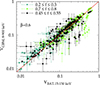 |
Fig. A.1. Comparison between estimates of variability obtained with BAT in the 15–150 keV band vs. the GBM estimates in the 8–900 keV band, obtained for a common sample with significant measures of variability. Three different ranges for f are shown. |
By assuming, for each energy channel, the geometric mean E of its boundary values and fitting the three points of each GRB and each combination of f and β values with a power-law, V ∝ Eα, we obtained an acceptable fit for 82% of cases. The corresponding α distribution is shown in Figure A.2 for three different ranges of f. Most values differ from zero by a relatively small amount, with a median value αmed = 0.13 and [0.0, 0.24] as interquartile range, when all values of f are included.
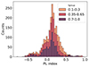 |
Fig. A.2. Distributions of the PL index α that models the dependence of variability on photon energy as V ∝ Eα for a sample of 44 GRB shared by BAT and GBM having significant measures of Vf for all of the three energy passbands (15–150, 8–150, and 150–900 keV). The three stacked histograms refer to three different ranges for f. |
We used this result to study the impact of using the two measures of Vf obtained with the full passbands of both BAT and GBM interchangeably: we derived the distribution of the ratio ξ between Vf calculated at 47 keV and Vf calculated at 85 keV, corresponding to the geometric mean energy of the 15–150 and of the 8–900 keV passbands, respectively. The median value is ξmed = 1.08, with 0.82 and 1.24 as the 5% and 95% quantiles, respectively. This can be summarised as a ≲20% discrepancy for most measures of Vf obtained with BAT and with GBM.
Appendix B: Comparison and test with past results
As anticipated in Section 4.2, we concluded that the correlation between Liso and Vf that was found in the early years by R01 and confirmed by G05 was possibly an artefact caused by the poor sampling of the Liso–Vf space.
Here we investigate the reason why the evidence for correlation was stronger for the smaller sample of G05: this is easily understood by looking at Figure B.1: in the region with low Vf and high Liso there is only one old GRB (000210). It is possible to identify a power-law (dashed line) below which all old GRBs but 000210 lie: Liso = (3 × 1049 erg s−1) (Vf/0.006)3.8. The slope of this power-law, 3.8, is also consistent with the slope  that was found by R01 to describe the relation between Liso and Vf. Assuming that the distribution of the old G05 GRBs in the Vf–Liso space is the same as the one of BAT and GBM GRBs, we estimated the probability that all of the 25, except for one at most, lie on the same side of the power-law by accident: 42/184 from the joint BAT-GBM sample lie above the boundary power-law. Assuming p = 42/184 = 22.8% as the probability for a single GRB to lie on the left side, the corresponding odds that at least 24 out of 25 lie on the same side of the dividing line are easily calculated with a two-sided binomial test11 and are 3%, so not impossible. Also, considering that the dividing line was found a posteriori, the correct odds are likely somewhat greater. In fact, a Kolmogorov-Smirnov 2-D test12 in the log Vf–log Liso plane between our set and the G05 one yields a p-value of 21%, which confirms the absence of evidence for a different parent distribution.
We conclude that stronger evidence for the Vf–Liso correlation that was found in the early years was the result of a poor sampling of the Vf–Liso plane.
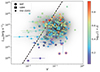 |
Fig. B.1. Same as Figure 4 with an additional dashed line that shows the region below which all but one old points lie. |
All Tables
Correlation coefficients of the Vf–Liso relation for the joint BAT-GBM sample, assuming β = 0.6.
All Figures
|
Fig. 1. Calculation of the variability. We show the 15–150-keV light curve {ri} of GRB 080319B as observed with BAT. The orange line shows the smoothed profile {sf, i} obtained with a smoothing timescale of Tf = 18.43 s, which collects a fraction f = 0.45 of the total fluence of the GRB. |
| In the text | |
|
Fig. 2. Comparison between variability estimates obtained with BAT in the 15–150 keV band vs. the GBM estimates in the 8–900 keV band, obtained for a common sample and assuming f = 0.45 and β = 0.6. Equality is shown by the solid line. |
| In the text | |
|
Fig. 3. Variability–luminosity correlation obtained for f = 0.8 and β = 0.6. This value of f gives the highest degrees of correlation. Different symbols refer to the different detectors used to measure Vf. For BAT-GBM shared GRBs, we used BAT values. Pentagons represent long-duration merger candidates. The redshift information is also available through the colour-coded scale. |
| In the text | |
|
Fig. 4. Variability–luminosity correlation obtained for f = 0.45 and β = 0.6. In addition to the 184 GRBs analysed in the present work, we also show (stars) GRBs from G05. The redshift is colour-coded. The shaded region shows a density map, obtained using a kernel density estimate, of the same data set (excluding the G05 GRBs). The four GRBs with red pentagons are long-duration merger candidates (GRB 060614, GRB 191019A, GRB 211211A, and GRB 230307A) that were considered separately. |
| In the text | |
|
Fig. 5. Same plot as Figure 4, except for the colour-code, which corresponds to five different classes of number of peaks. |
| In the text | |
|
Fig. 6. Collection of six observer-frame GRBs with medium to high luminosity and low variability. Each panel reports the GRB name along with the (Vf, log Liso) pair. All of them are BAT bursts (15–150 keV), except for BeppoSAX GRB 000210 (40–700 keV) in the bottom right panel. In the case of BAT LCs, the count rates are expressed in count s−1 per fully illuminated detector for an equivalent on-axis source. |
| In the text | |
|
Fig. 7. Collection of ten observer-frame GRBs with high variability, Vf > 0.1, and relatively low luminosity, Liso ≲ 1052 erg s−1. Each panel reports the GRB name along with the (Vf, log Liso) pair. All of them are BAT bursts (15–150 keV), except for Fermi GRB 140623A (8–900 keV). In the case of BAT LCs, the count rates are expressed in count s−1 per fully illuminated detector for an equivalent on-axis source. |
| In the text | |
|
Fig. 8. MVT vs. variability for a subsample of 184 GRBs. The pentagons show the four long-duration merger candidates. The MVT values were calculated as in Camisasca et al. (2023a). Liso is colour-coded. |
| In the text | |
|
Fig. A.1. Comparison between estimates of variability obtained with BAT in the 15–150 keV band vs. the GBM estimates in the 8–900 keV band, obtained for a common sample with significant measures of variability. Three different ranges for f are shown. |
| In the text | |
|
Fig. A.2. Distributions of the PL index α that models the dependence of variability on photon energy as V ∝ Eα for a sample of 44 GRB shared by BAT and GBM having significant measures of Vf for all of the three energy passbands (15–150, 8–150, and 150–900 keV). The three stacked histograms refer to three different ranges for f. |
| In the text | |
|
Fig. B.1. Same as Figure 4 with an additional dashed line that shows the region below which all but one old points lie. |
| In the text | |
Current usage metrics show cumulative count of Article Views (full-text article views including HTML views, PDF and ePub downloads, according to the available data) and Abstracts Views on Vision4Press platform.
Data correspond to usage on the plateform after 2015. The current usage metrics is available 48-96 hours after online publication and is updated daily on week days.
Initial download of the metrics may take a while.