| Issue |
A&A
Volume 685, May 2024
|
|
|---|---|---|
| Article Number | A34 | |
| Number of page(s) | 7 | |
| Section | Extragalactic astronomy | |
| DOI | https://doi.org/10.1051/0004-6361/202449200 | |
| Published online | 01 May 2024 | |
Distribution of the number of peaks within a long gamma-ray burst
1
Department of Physics and Earth Science, University of Ferrara, Via Saragat 1, 44122 Ferrara, Italy
2
INFN – Sezione di Ferrara, Via Saragat 1, 44122 Ferrara, Italy
e-mail: This email address is being protected from spambots. You need JavaScript enabled to view it.
3
INAF – Osservatorio di Astrofisica e Scienza dello Spazio di Bologna, Via Piero Gobetti 101, 40129 Bologna, Italy
4
Department of Physics, University of Cagliari, SP Monserrato-Sestu, km 0.7, 09042 Monserrato, Italy
5
Ioffe Institute, Politekhnicheskaya 26, 194021 St. Petersburg, Russia
6
INAF – Osservatorio Astronomico d’Abruzzo, Via Mentore Maggini snc, 64100 Teramo, Italy
7
Key Laboratory of Particle Astrophysics, Institute of High Energy Physics, Chinese Academy of Sciences, Beijing 100049, PR China
8
University of Chinese Academy of Sciences, Beijing 100049, PR China
Received:
10
January
2024
Accepted:
23
February
2024
Abstract
Context. The variety and complexity of long duration gamma-ray burst (LGRB) light curves (LCs) encode a wealth of information about the way LGRB engines release their energy following the collapse of the progenitor massive star. Thus far, attempts to characterise GRB LCs have focused on a number of properties, such as the minimum variability timescale and power density spectra (both ensemble average and individual), or considering different definitions of variability. In parallel, a characterisation as a stochastic process has been pursued by studying the distributions of waiting times, peak flux, and fluence of individual peaks that can be identified within GRB time profiles. However, an important question remains as to whether the diversity of GRB profiles can be described in terms of a common stochastic process.
Aims. Here, we address this issue by extracting and modelling, for the first time, the distribution of the number of peaks within a GRB profile.
Methods. We analysed four different GRB catalogues: CGRO/BATSE, Swift/BAT, BeppoSAX/GRBM, and Insight-HXMT. The statistically significant peaks were identified by means of well tested and calibrated algorithm MEPSA and further selected by applying a set of thresholds on the signal-to-noise ratio. We then extracted the corresponding distributions of number of peaks per GRB.
Results. Among the different models considered (power-law, simple or stretched exponential), we find that only a mixture of two exponentials was able to model all the observed distributions. This suggests the existence of two distinct behaviours: (i) an average number of 2.1 ± 0.1 peaks per GRB (“peak-poor”), accounting for about 80% of the observed population of GRBs; and (ii) an average number of 8.3 ± 1.0 peaks per GRB (“peak-rich”), accounting for the remaining 20% of the observed population.
Conclusions. We associate the class of peak-rich GRBs with the presence of sub-second variability, which appears to be surprisingly absent among peak-poor GRBs. The two classes could result from two distinct regimes in which the inner engines of GRBs release their energy or otherwise dissipate that energy as gamma rays.
Key words: methods: data analysis / methods: statistical / gamma-ray burst: general
© The Authors 2024
 Open Access article, published by EDP Sciences, under the terms of the Creative Commons Attribution License (https://creativecommons.org/licenses/by/4.0), which permits unrestricted use, distribution, and reproduction in any medium, provided the original work is properly cited.
This article is published in open access under the Subscribe to Open model. This email address is being protected from spambots. You need JavaScript enabled to view it. to support open access publication.
1. Introduction
Gamma-ray burst (GRB) prompt emission is observed in at least two kinds of explosive transients: (i) the merger of a compact object binary system (Eichler et al. 1989; Paczynski 1991; Narayan et al. 1992; Abbott et al. 2017) and (ii) the core collapse of some kinds of massive stars also known as “collapsar” (Woosley 1993; Paczyński 1998; MacFadyen & Woosley 1999; Yoon & Langer 2005). While the prompt emission duration remains the strongest hint on the nature of the progenitor, in a few cases it turned out to be deceitful. To avoid confusion, the two progenitor families (i) and (ii) are often referred to as type-I and type-II GRBs, respectively (Zhang 2006). In this work, we focus on the latter class.
Modelling the thousands of GRB prompt emission time-resolved spectra has indicated that the observed variety is likely the result of different radiative processes in different GRBs, given the variety of spectral components that are observed: the non-thermal Band function, an occasional quasi-thermal component, and even a broad-band power-law (see Kumar & Zhang 2015 for a review). These processes are possibly related to different dissipation mechanisms taking place at different distances from the progenitor and driven by key properties, such as the ejecta composition of the relativistic jet that is launched by the GRB inner engine.
In parallel, while numerous studies that focused on the temporal properties of GRB time profiles have contributed to characterise their variability, the broad variety and highly erratic nature of GRB prompt emission remains mostly unexplained and apparently disconnected from the properties that are inferred from the afterglow modelling, apart from the energetics. Despite being affected by a large scatter, a positive correlation between peak luminosity and variability was found as soon as the number of bursts with measured redshift increased to a dozen or more (Reichart et al. 2001; Fenimore & Ramirez-Ruiz 2000). Variability was defined as the net (that is, removed of the counting statistics noise contribution) variance of the light curve (LC) with respect to a smoothed version of the same. The correlation was later confirmed over larger data sets, along with its large scatter (Guidorzi et al. 2005, 2006; Guidorzi 2005), with a forthcoming analysis of Swift and Fermi GRBs (Guidorzi et al. in prep.). Peak luminosity was also found to be correlated with the so-called minimum variability timescale (MVT), defined as the shortest timescale over which an uncorrelated flux change is observed significantly in excess of statistical fluctuations (see Camisasca et al. 2023 and references therein). A possible interpretation explains more variable GRBs as the result of narrower jets with higher Lorentz factors and shorter spreading timescales than wider jets (Kobayashi et al. 2002).
Most GRB LCs can be described as a sequence of peaks of different shapes, duration, and intensity with no clear rule. While different techniques have revealed that temporal power is generally distributed over a broad range of timescales (from ∼10 ms to several 10 s), two distinct components were also identified in a number of GRBs: slow (≳1 s), and fast (down to few 10 ms; Vetere et al. 2006; Gao et al. 2012; Guidorzi et al. 2016). Since the first catalogues of the Burst And Transient Source Experiment (BATSE; Paciesas et al. 1999) that flew aboard the Compton Gamma-Ray Observatory (CGRO; 1991–2000), distributions of properties of the peaks (seen as building blocks of the prompt emission) were studied in detail (e.g. see Ramirez-Ruiz & Merloni 2001; Quilligan et al. 2002; Nakar & Piran 2002). However, despite the enormous progress in the knowledge of GRB progenitors and their environments, a precise characterisation of the stochastic process(es) that drive(s) GRB engines in releasing their energy as a function of time is missing. Hence, the degree of complexity exhibited by a given GRB LC, especially if it is seen as a point process given by the sequence of peaks with different intensities and durations, can hardly be translated into clues on the nature of its inner engine or on the nature of the powering mechanism that rules its evolution.
In this respect, while the distribution of the number of peaks per GRB was obtained in past investigations (e.g. Quilligan et al. 2002; Guidorzi et al. 2016), to our knowledge, no attempt to model and interpret it has been done to date. Following previous analogous definitions (Li & Fenimore 1996; Nakar & Piran 2002), a “peak” is defined as a statistically significant increase of the count rate with respect to the neighbouring time bins, using the terminology introduced by Li & Fenimore (1996). In this work we addressed this by applying a well tested peak identification code, MEPSA (Guidorzi 2015), to four independent catalogues among the different past and present missions aimed at GRB studies (Tsvetkova et al. 2022): CGRO/BATSE, Swift/BAT, BeppoSAX/GRBM, and Insight-HXMT. A forthcoming paper reports on the ongoing analysis of Fermi/GBM GRBs, although some preliminary results are mentioned in the following. We note that our aim deliberately neglects the temporal structures of peaks, which might differ significantly from one another, or how much they overlap in time, provided that they can be identified as distinct peaks. Section 2 reports the data sets used, the LC extraction along with the peak identification. Section 3 reports the results of the analysis, which are then discussed in Sect. 4.
2. Data sets
We obtained the background-subtracted LC of GRBs with a bintime of 64 ms (except for BeppoSAX/GRBM for which we made use of both 1-s and 62.5-ms bin times) and extracted a list of peaks detected with MEPSA, a code specifically devised and optimised to identify peaks in uniformly sampled and background-subtracted GRB LCs (Guidorzi 2015), discarding candidates with a signal-to-noise ratio of S/N < 5.
From the BATSE 4B catalogue (Paciesas et al. 1999) we took the 64-ms time profiles of LGRBs (T90 > 2 s) made available by the BATSE team1. Taken with the eight BATSE Large Area Detectors (LADs), these time profiles resulted from the concatenation of three standard BATSE types, DISCLA, PREB, and DISCSC. They are available in four energy channels, 25−55, 55−110, 110−320, and > 320 keV: we used the summed counts over the four channels. The background was interpolated with polynomials of up to fourth degree as prescribed by the BATSE team. These background-subtracted profiles were then processed with MEPSA and we selected the GRBs with at least one significant peak. We ended up with a sample of 1457 GRBs, which hereafter are referred to as the BATSE sample.
We started from all the GRBs detected by Swift/BAT in burst mode from January 2005 to July 2023 and rejected those with T90 ≤ 2 s, as well as the long-lasting type-I candidates, since they had been classified by the Swift team; these include all the so-called short extended-emission GRBs (Norris & Bonnell 2006), in addition to peculiar events like 060614, 211211A (Gehrels et al. 2006; Yang et al. 2022). The information on the T90 duration and on the LC characterisation was taken either from the BAT3 catalogue (Lien et al. 2016), when available, or from the Swift/BAT team circulars. For each burst we extracted the mask-weighted, 64-ms bin time profile in the 15−150 keV passband following the standard procedure recommended by the BAT team2 and applied MEPSA. Imposing the above-mentioned S/N > 5 threshold on the peak candidates, we selected all the type-II GRB candidates with at least one peak and ended up with 1277 bursts. Hereafter, this is referred to as the BAT sample.
The LCs available in the 40−700 keV passband for the GRBs from the BeppoSAX/GRBM catalogue (Frontera et al. 2009) come after two fashions: for the 2/3 that triggered the on-board logic, a 7.8125-ms profile covering the first 106 s for each of the four independent units is available. For the remaining 1/3, only 1-s LCs are available. For the former we obtained 62.5-ms profiles. The GRBs observed before November 1996 were ignored due to the presence of extra-Poissonian noise in the background rate of the GRBM, which was removed after raising the LLT energy threshold (Frontera et al. 2009). We then discarded short GRBs (T90 < 2 s, as reported by Frontera et al. 2009) and ran MEPSA on the LC of the most illuminated detector (or on the sum of the two most illuminated ones, depending on which LC had the higher S/N) independently on both 62.5-ms and 1-s profiles and merged the results, making sure to count once the peaks that triggered both timescales. The reason of this strategy is not to lose peaks that occurred after the first 106 s acquired with high temporal resolution. We applied the same S/N > 5 threshold as for the other catalogues and ended up with 820 GRBs with at least one significant peak, which hereafter are referred to as the BeppoSAX sample.
From the first Insight-HXMT/HE GRB catalogue (Song et al. 2022) we discarded all the GRBs with T90 < 2 s, as well as those belonging to the iron sample, for which the electronics saturated due to excessively high count rates. For the remaining GRBs we extracted the 64-ms, dead-time corrected LCs obtained by summing the counts of all the 18 HE detector units, selecting only the CsI events (for which the HE works as an open-sky monitor) following the procedure described in Song et al. (2022). The total energy passband depends on the HE operation mode: either 80−800 or 200−3000 keV for the normal and GRB (or low-gain) mode, respectively. The background interpolation and subtraction was carried out as in Camisasca et al. (2023), to which the reader is referred. We finally ran MEPSA and after applying the same S/N > 5 selection we ended up with 202 GRBs hosting at least one significant peak. Hereafter, these GRBs are referred to as the Insight-HXMT sample.
3. Results
For each data set, we obtained the distribution of the number of peaks per GRB, expressed as number of GRBs having n peaks, as a function of n for all integer values (n ≥ 1). This is clearly a discrete distribution. For each of the models considered below, we first determined the best fit parameters by maximising the corresponding likelihood function. We then estimated the parameters’ marginalised distributions by sampling the posterior distribution using Markov chain Monte Carlo (MCMC) sampling with EMCEE (Foreman-Mackey et al. 2013): starting from the maximum likelihood solution, we ran 32 walkers for 5000 steps and discard the first 100 steps as burn-in. We tested the goodness of the best solution by grouping the expected number of GRBs so as to have at least five per class and carried out a χ2 test.
We first tried to model the distributions with a discrete simple exponential, which is mostly determined by the majority of GRBs, which have 1 or 2 peaks. However, all data sets showed an excess of GRBs with many (≳10) peaks. Motivated by the possible presence of a hard tail, we then considered a simple power-law model, but the result was poor. A broken power-law did not provide satisfactory fits for all data sets either.
As a further attempt, we considered a stretched exponential (also known as the empirical Kohlrausch–Williams–Watts, or KWW, function), which is often encountered in several contexts in physics for modelling relaxation processes of systems that dissipate energy and are initially out of equilibrium (e.g. see Lukichev 2019, and references therein). It can also result from the combination of numerous (ideally continuous) exponentially distributed processes (Johnston 2006). Moreover, a stretched exponential was found to describe the average temporal decay of peak-aligned and peak-normalised profiles of BATSE GRBs (Stern & Svensson 1996). As a result, only the distribution of the BATSE sample, which is the most numerous one, could not be modelled satisfactorily with a stretched exponential (χ2 test p-value of 10−6).
Finally, we considered the mixture of two simple exponentials with the relative weight treated as a free parameter. Specifically, the fraction f(n) of GRBs hosting n peaks is described by via
 (1)
(1)
where k is a normalisation constant, such that  , ni (i = 1, 2) is the characteristic number of peaks per GRB of the ith component (n1 ≤ n2 by convention) and ξ is a relative normalisation parameter, thereby amounting to three free parameters. Due to the discrete nature of the distribution, the corresponding expected number of peaks per GRB of the ith exponential component, ⟨n(i)⟩, is not simply ni (as in the case of a continuous distribution) but instead:
 (2)
(2)
Hereafter, Eq. (1) is referred to as the mixture model of two exponentials (M2E).
The resulting distributions along with the best fit M2Es are shown in Fig. 1, while Table 1 reports the best fit values of the model parameters and the corresponding p-value of the χ2 test. All of the four data sets can be satisfactorily modelled and, what is more, the parameters values are similar to each other, despite the different effective areas and energy passbands. We also performed a joint fit of all the four distributions with a common set of parameters in two ways: (i) by merging all GRBs and treating it as a single data set, thus dominated by the richest data sets; and (ii) by keeping the four distributions separate and assigning equal weights in the total likelihood. It was only for (i) that we obtained a marginally acceptable solution (p-value of 3%, see Table 1).
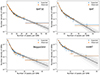 |
Fig. 1. Distributions of number of GRBs per number of peaks for different catalogues: CGRO/BATSE (top left), Swift/BAT (top right), BeppoSAX/GRBM (bottom left), and Insight-HXMT (bottom right). Observed data and expected counts are shown in orange and blue, respectively. All histograms have been grouped so as to ensure a minimum number of counts per bin. Dashed lines show the best mixture model of two exponentials that fit each distribution. Grey models are the result of a random sampling of the posterior distribution of the parameters as determined via MCMC. |
We also calculated the fraction of GRBs  contributed by the second exponential component, according to each best fit solution. This is calculated simply as:
 (3)
(3)
Interestingly, all data sets have compatible values, with a weighted average of 0.19 ± 0.03 (90% confidence). Analogous results are found for the expected numbers of peaks of either component: while the first component presents a range of values for ⟨n(1)⟩ only marginally compatible with each other (weighted average of 2.1 ± 0.1, p-value of 6 × 10⁻⁶), the expected value for the second component, ⟨n(2)⟩, is compatible among all data sets, with a weighted average of 8.3 ± 1.0 (p-value of 0.06). Hereafter, the first (i = 1) and the second (i = 2) components are referred to as the peak-poor and the peak-rich ones, respectively. Similar results were obtained on a preliminary sample of 393 Fermi Gamma-ray Burst Monitor (GBM; Meegan et al. 2009) GRBs, 361 of which are shared with the BAT sample (Maccary et al., in prep.); in particular, we found a peak-rich fraction  , which is in line with the other four samples.
We investigated the relation between number of peaks per GRB n and burst duration as expressed in terms of T90, whose values were taken from the official corresponding catalogue papers. Figure 2 shows the results for all catalogues. We studied how the median and the logarithmic mean of T90 of all catalogues merged together vary as a function of n. To avoid low-count fluctuations in the median and mean estimates, we grouped bins of n so as to have at least 9 GRBs per class. The two quantities clearly track each other very closely (Fig. 2). Interestingly, the dependence of T90 on n becomes shallower for n ≳ n2; when modelling the median value of T90,  , with a power-law,
  , we found a = 0.58 (κ = 18.8) for n < n2, while a = 0.39 (κ = 23.0) for n > n2 (dash-dotted magenta line in Fig. 2). The fact that a significantly differs from 1 suggests that the abundance of peaks within a GRB is not compatible with a common probability per unit time of emitting a peak, which would predict a ∼ 1. Moreover, the dynamic range of
  (19 s for n = 1, 57 s for 50 < n < 85) is significantly narrower than the scatter of T90 for any n: this indicates that T90 is not a main driver of n. In addition, the fact that the dependence of
  becomes even shallower for large values n, where most GRBs are contributed by the peak-rich component of Eq. (1), further supports the possible existence of two families of GRBs or (at least) two different behaviours for the GRB engines.
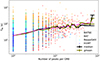 |
Fig. 2. T90 vs. number of peaks per GRBs for the different data sets. Also shown: the T90 median (black) and the geometric mean (olive) as a function of number of peaks, grouped with at least nine GRBs each. The dashed-dotted line (magenta) shows a broken power-law fit of the median behaviour. |
3.1. Instrumental selection effects
The number of peaks clearly depends on the detector sensitivity and on the threshold on the S/N values. Secondly, it also depends on the energy passband, given that harder channels exhibit narrower and spikier temporal structures than softer channels. This is clearly shown by the higher number of peaks in the BATSE sample compared with the other samples and is due to the better sensitivity of the former instrument.
We investigated the impact of S/N by repeating the analysis assuming two additional threshold values: S/N > 7 and S/N > 9. The total number of identified peaks decreased to a fraction between 70 and 85% for the different catalogues, when moving from S/N > 5 to S/N > 9. Only the average number of peaks per GRB of the BATSE sample decreased from 5.6 to 4.9, whereas for all the other samples the same quantity remained in the range 2.8 − 3.0 peaks per GRB. The reason is that for the other three samples the number of GRBs featuring at least one significant peak decreased proportionally, due to a lower sensitivity with respect to BATSE. Because of this, the weighted average number of peaks per GRB of both peak-poor and peak-rich components did not change significantly: ⟨n(1)⟩ passed from 2.1 ± 0.1 (S/N > 5) to 2.0 ± 0.1 (S/N > 9). ⟨n(2)⟩ changed from 8.3 ± 1.0 (S/N > 5) to 8.1 ± 1.0 (S/N > 9). Finally, the fraction of peak-rich GRBs moved from 0.19 ± 0.03 (S/N > 5) to 0.22 ± 0.03 (S/N > 9). Overall, while the number of peaks per GRB is inevitably expected to decrease by keeping raising the S/N threshold (although in a limited way, as we found passing from 5 to 9), the fractions of peak-poor and peak-rich GRBs do not seem to depend sensitively on the S/N threshold.
We identified 160 GRBs in common between the BATSE and the BeppoSAX samples. For each of these GRBs we calculated the difference between the number of peaks detected from the two profiles, Δn = n(BATSE) − n(SAX). We divided this common sample into two subsamples: the GRBs for which there are high-resolution (HR; 62.5-ms) data, and the GRBs with only 1-s data from BeppoSAX. Figure 3 shows the distributions of Δn for different S/N thresholds. First, the distributions do not depend significantly on the S/N threshold. Secondly, on average, the presence of HR data from BeppoSAX does not appreciably impact the number of detected peaks. Thirdly, the median values in all cases is +2, which reflects the better sensitivity of BATSE. In addition, ∼60% (∼70%) of all common GRBs have |Δn|≤2 (|Δn|≤3). A discrepancy of ∼2 − 3 in estimating n is small compared with ⟨n(2)⟩−⟨n(1)⟩≃6.2 ± 1.0. We derived the analogous distribution for the preliminary common sample of 361 GRBs shared by BAT and Fermi/GBM, confirming that for the majority of bursts the difference in the number of peaks is small: 86% and 92% GRBs with |Δn|≤2 and |Δn|≤3, respectively (Maccary et al., in prep.). Consequently, for most GRBs, the probability of belonging to either the peak-poor or the peak-rich family does not crucially depend on the detector used, at least as long as these catalogues are concerned. A more thorough characterisation through mapping with other GRB observed properties goes beyond the scope of the present analysis and merits a separate investigation.
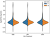 |
Fig. 3. Distributions of Δn, defined as the difference between the number of peaks detected with BATSE and the one detected with BeppoSAX for a common sample of 160 GRBs, for three different thresholds on S/N. Blue and orange show the subsamples of GRBs with/without BeppoSAX high-resolution data, respectively. |
3.2. Number of peaks versus peak luminosity
According to the variability-luminosity relation, more luminous GRBs are (on average) more variable. We therefore studied the relation between number of peaks and peak luminosity. To this aim, we selected 17 GRBs from the BeppoSAX and 131 from the BAT samples with spectroscopically measured redshift and for which the isotropic-equivalent peak luminosity, Lp, iso, in the comoving-frame 1 − 104 keV passband had been estimated with broadband experiments, such as BeppoSAX and Konus/WIND. These values were taken from Ghirlanda et al. (2005), Amati et al. (2008), Yonetoku et al. (2010), Dichiara et al. (2016), Tsvetkova et al. (2017, 2021). Figure 4 shows the result. Non-parametric Spearman’s and Kendall’s correlation tests over the joint sample of 148 GRBs yielded a null hypothesis probability of no correlation as small as 1.1 × 10⁻⁷ and 2.0 × 10⁻⁷, respectively. Hence, even though it is highly dispersed, the correlation is statistically significant, with peak-rich GRBs being, on average, more luminous.
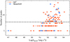 |
Fig. 4. Number of peaks vs. isotropic-equivalent peak luminosity Lp, iso for a sample of 131 (17) GRBs with known z from the BAT (BeppoSAX) samples. The dashed line marks the median number of peaks of the whole sample. |
As a further check, we also split the sample based on the median number of peaks of n = 3 of the joint sample, ending up with 79 (69) GRBs with n ≤ 3 (n > 3) peaks. The two groups can be roughly considered as peak-poor and peak-rich samples. Median peak luminosities are 1.5 × 1052 and 6.8 × 1052 erg s−1 for the peak-poor and peak-rich samples, respectively. The probability of a common parent population for the two distributions of Lp, iso is 9 × 10⁻⁵ and < 10−3 according to the Kolmogorov–Smirnov and Anderson–Darling tests3, respectively. In conclusion, robust evidence is found that peak-rich GRBs are, on average, more luminous than peak-poor ones, although the two peak luminosity distributions are strongly overlapped.
4. Discussion and conclusions
The analysis of a former Swift/BAT sample of GRB LCs showed that the power density spectra of peak-rich GRBs tend to be preferentially described by a shallow PL, which is the result of the superposition of peaks covering a broad range of timescales, such that no dominant timescale emerges (see Fig. 7 of Guidorzi et al. 2016). In particular, peak-rich GRBs tend to have relatively more temporal power on shorter (≲1 s) timescales than peak-poor GRBs due to the presence of a number of narrow peaks which are mostly absent in peak-poor GRBs. An illustrative example of this difference is shown in Fig. 5: two bursts from the BeppoSAX/GRBM catalogue having comparable fluence and peak flux, one with just two peaks and a long smooth decaying tail (T90 ∼ 140 s), while the other featuring 24 peaks within a T90 = 60 s, most of which have subsecond durations.
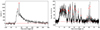 |
Fig. 5. Examples of two GRBs having only 2 (left, 981203A) and 24 peaks (right, 010412), respectively, as observed in the 40−700 keV passband by BeppoSAX/GRBM. The red points show the identified peaks, while dashed lines show the interpolated background. The fluence and peak flux of the two GRBs are very similar (Frontera et al. 2009). |
In light of the results here reported on the possible existence of two distinct dynamics, as revealed by the distribution of number of peaks per GRB, the emerging picture is suggestive of two kinds of regimes through which type-II GRB engines release their energy: (i) one emitting a few (∼2.1 on average) typically broad peaks (≳1 s), making up ∼80% of the observed population of GRBs of past and present catalogues; and (ii) the other one emitting several peaks (∼8.3 on average), covering a broader range of timescales, including subsecond ones, which makes up the remaining 20% of the observed population. The coexistence of two kinds of timescales in some GRBs (i.e. the so-called slow and fast variability components) has already been suggested in the literature (Vetere et al. 2006; Margutti 2009; Gao et al. 2012; Guidorzi et al. 2016). Our results suggest a further characterisation, which points to the existence of two distinct ways GRB engines may work.
We may look at the class of peak-rich GRBs as being characterised by the presence of a fast component that manifests itself through a number of narrow peaks, which are instead mostly missing in the other class of peak-poor GRBs. Peak richness is also preferentially accompanied (on average) by shorter MVT and higher peak luminosity, although the latter alone cannot be used to discriminate between the two classes, given the strong overlap shown in Fig. 4. The origin of the fast component in the literature has been investigated within the context of different progenitor models and can be summarised in two main groups, depending on whether the fast component (a) reflects the inner engine activity or (b) is mainly driven by other factors. Within the context of the internal shock (IS) model (Kobayashi et al. 1997; Daigne & Mochkovitch 1998; Maxham & Zhang 2009), the number of peaks and the sequence of time intervals simply reflect the emission time history of the inner engine. Unlike the slow one, the fast component imprinted by the inner engine would not be quenched, as a purely hydrodynamic jet propagates through the stellar envelope (Morsony et al. 2010). When the possibility of a magnetised outflow is considered, a weakly magnetised and intermittent jet, which is less subject to mixing with the surrounding progenitor gas than a pure hydrodynamic jet, appears more promising to explain the observed variability, since the predicted GRB emission would be less inhibited (Gottlieb et al. 2020b, 2021).
Within the (a) scenario, our results suggest that either inner engines of peak-poor GRBs are quieter, especially at short timescales, or their progenitor structure is able to suppress the subsecond variability. This could be due to the different degree of magnetisation of the jet, which can affect the mixing and consequently the jet baryon load (Gottlieb et al. 2020a). There are a number of interpretations of how a GRB engine, such as an accreting black hole (BH), could explain the fast component; for example, this can be caused by the fluctuations of the viscosity parameter and how they consequently propagate through the disk in a similar way to what is believed in the case of BH binaries and active galactic nuclei (Lin et al. 2016). Alternatively, they could be caused by the fastest modes of magneto-rotational instabilities that drive and launch a magnetised jet through the Blandford-Znajek process (Janiuk et al. 2021). Within these contexts, peak-poor GRBs could be indicative of a regime in which either viscosity fluctuations or fast instabilities are strongly inhibited.
In the alternative (b) scenario, the fast component that characterises peak-rich GRBs originates at further distance from the inner engine, up to the GRB emission site. In the Internal-Collision induced MAgnetic Reconnection and Turbulence (ICMART) model (Zhang & Yan 2011), a wind of moderately magnetised shells (with magnetisation 1 ≲ σ ≲ 100 at the GRB site) collide and produce several runaway cascades of magnetic reconnection events. The fast component would be the result of turbulent, Doppler-boosted emission of mini-jets within the comoving frame of the colliding shells, caused by particles accelerated by magnetic reconnections. Simulations carried out by Zhang & Zhang (2014) show that spikier GRB LCs with many distinguishable peaks are, in particular, favoured by the following factors: (1) large emission site (R ≳ 1015 cm) from the progenitor giving a longer curvature decay tail, which thus does not wash out the rapid variability due to the mini-jets; and (2) a more magnetised outflow, which corresponds to a higher contrast between the Lorentz factors of the mini-jets and that of the corresponding shell. Our results could suggest that the turbulent magnetic reconnection regime either sets in efficiently (peak-rich GRB) or it does not (peak-poor GRB).
Ultimately, the possibility remains that the two classes reflect two different kinds of inner engines, such as ms-magnetars and accreting BHs, for which other potentially discriminating signatures in the prompt emission are yet to be identified.
A final note concerns the long-lasting GRBs that are type-I candidates, such as 060614, 211211A, and 230307A (Gehrels et al. 2006; Yang et al. 2022; Troja et al. 2022; Gompertz et al. 2023; Dichiara et al. 2023; Levan et al. 2024), which were ignored in the present analysis; we note that all their LCs exhibit numerous peaks (several dozens). While peak-richness alone cannot be a distinctive feature of this kind of merger candidates – given that there are several type-II GRBs with an associated SN that are also peak-rich (e.g. 080319B, Racusin et al. 2008) – nevertheless it could be interpreted as a clue to understanding the nature of the inner engine powering these mergers.
These tests were done using scipy.stats.ks_2samp and scipy.stats.anderson_ksamp, respectively.
Acknowledgments
We acknowledge the anonymous reviewer for a constructive report which improved the manuscript. C.G. acknowledges the Dept. of Physics and Earth Science of the University of Ferrara for the financial support through the “FIRD 2022” grant. M.B. is supported by the Dept. of Physics and Earth Science at the University of Ferrara through the FIRD 2022 grant. A.T. acknowledges financial support from “ASI-INAF Accordo Attuativo HERMES Pathinder operazioni n. 2022-25-HH.0” and the basic funding program of the Ioffe Institute FFUG-2024-0002.
References
- Abbott, B. P., Abbott, R., Abbott, T. D., et al. 2017, ApJ, 848, L13 [CrossRef] [Google Scholar]
- Amati, L., Guidorzi, C., Frontera, F., et al. 2008, MNRAS, 391, 577 [Google Scholar]
- Camisasca, A. E., Guidorzi, C., Amati, L., et al. 2023, A&A, 671, A112 [NASA ADS] [CrossRef] [EDP Sciences] [Google Scholar]
- Daigne, F., & Mochkovitch, R. 1998, MNRAS, 296, 275 [NASA ADS] [CrossRef] [Google Scholar]
- Dichiara, S., Guidorzi, C., Amati, L., Frontera, F., & Margutti, R. 2016, A&A, 589, A97 [NASA ADS] [CrossRef] [EDP Sciences] [Google Scholar]
- Dichiara, S., Tsang, D., Troja, E., et al. 2023, ApJ, 954, L29 [NASA ADS] [CrossRef] [Google Scholar]
- Eichler, D., Livio, M., Piran, T., & Schramm, D. N. 1989, Nature, 340, 126 [NASA ADS] [CrossRef] [Google Scholar]
- Fenimore, E. E., & Ramirez-Ruiz, E. 2000, arXiv e-prints [arXiv:astro-ph/0004176] [Google Scholar]
- Foreman-Mackey, D., Hogg, D. W., Lang, D., & Goodman, J. 2013, PASP, 125, 306 [Google Scholar]
- Frontera, F., Guidorzi, C., Montanari, E., et al. 2009, ApJS, 180, 192 [Google Scholar]
- Gao, H., Zhang, B.-B., & Zhang, B. 2012, ApJ, 748, 134 [NASA ADS] [CrossRef] [Google Scholar]
- Gehrels, N., Norris, J. P., Barthelmy, S. D., et al. 2006, Nature, 444, 1044 [NASA ADS] [CrossRef] [Google Scholar]
- Ghirlanda, G., Ghisellini, G., & Firmani, C. 2005, MNRAS, 361, L10 [NASA ADS] [Google Scholar]
- Gompertz, B. P., Ravasio, M. E., Nicholl, M., et al. 2023, Nat. Astron., 7, 67 [Google Scholar]
- Gottlieb, O., Bromberg, O., Singh, C. B., & Nakar, E. 2020a, MNRAS, 498, 3320 [NASA ADS] [CrossRef] [Google Scholar]
- Gottlieb, O., Levinson, A., & Nakar, E. 2020b, MNRAS, 495, 570 [NASA ADS] [CrossRef] [Google Scholar]
- Gottlieb, O., Bromberg, O., Levinson, A., & Nakar, E. 2021, MNRAS, 504, 3947 [NASA ADS] [CrossRef] [Google Scholar]
- Guidorzi, C. 2005, MNRAS, 364, 163 [NASA ADS] [CrossRef] [Google Scholar]
- Guidorzi, C. 2015, Astron. Comput., 10, 54 [NASA ADS] [CrossRef] [Google Scholar]
- Guidorzi, C., Frontera, F., Montanari, E., et al. 2005, MNRAS, 363, 315 [NASA ADS] [CrossRef] [Google Scholar]
- Guidorzi, C., Frontera, F., Montanari, E., et al. 2006, MNRAS, 371, 843 [NASA ADS] [CrossRef] [Google Scholar]
- Guidorzi, C., Dichiara, S., & Amati, L. 2016, A&A, 589, A98 [NASA ADS] [CrossRef] [EDP Sciences] [Google Scholar]
- Janiuk, A., James, B., & Palit, I. 2021, ApJ, 917, 102 [NASA ADS] [CrossRef] [Google Scholar]
- Johnston, D. C. 2006, Phys. Rev. B, 74, 184430 [NASA ADS] [CrossRef] [Google Scholar]
- Kobayashi, S., Piran, T., & Sari, R. 1997, ApJ, 490, 92 [Google Scholar]
- Kobayashi, S., Ryde, F., & MacFadyen, A. 2002, ApJ, 577, 302 [NASA ADS] [CrossRef] [Google Scholar]
- Kumar, P., & Zhang, B. 2015, Phys. Rep., 561, 1 [Google Scholar]
- Levan, A. J., Gompertz, B. P., Salafia, O. S., et al. 2024, Nature, 626, 737 [NASA ADS] [CrossRef] [Google Scholar]
- Li, H., & Fenimore, E. E. 1996, ApJ, 469, L115 [NASA ADS] [CrossRef] [Google Scholar]
- Lien, A., Sakamoto, T., Barthelmy, S. D., et al. 2016, ApJ, 829, 7 [Google Scholar]
- Lin, D.-B., Lu, Z.-J., Mu, H.-J., et al. 2016, MNRAS, 463, 245 [NASA ADS] [CrossRef] [Google Scholar]
- Lukichev, A. 2019, Phys. Lett. A, 383, 2983 [CrossRef] [Google Scholar]
- MacFadyen, A. I., & Woosley, S. E. 1999, ApJ, 524, 262 [NASA ADS] [CrossRef] [Google Scholar]
- Margutti, R. 2009, Toward New Insights on the Gamma-ray Burst Physics: From X-ray Spectroscopy to the Identification of Characteristic Time Scales (Milan: Università degli Studi Milano-Bicocca) [Google Scholar]
- Maxham, A., & Zhang, B. 2009, ApJ, 707, 1623 [CrossRef] [Google Scholar]
- Meegan, C., Lichti, G., Bhat, P. N., et al. 2009, ApJ, 702, 791 [Google Scholar]
- Morsony, B. J., Lazzati, D., & Begelman, M. C. 2010, ApJ, 723, 267 [NASA ADS] [CrossRef] [Google Scholar]
- Nakar, E., & Piran, T. 2002, MNRAS, 331, 40 [NASA ADS] [CrossRef] [Google Scholar]
- Narayan, R., Paczynski, B., & Piran, T. 1992, ApJ, 395, L83 [NASA ADS] [CrossRef] [Google Scholar]
- Norris, J. P., & Bonnell, J. T. 2006, ApJ, 643, 266 [NASA ADS] [CrossRef] [Google Scholar]
- Paciesas, W. S., Meegan, C. A., Pendleton, G. N., et al. 1999, ApJS, 122, 465 [NASA ADS] [CrossRef] [Google Scholar]
- Paczynski, B. 1991, Acta Astron., 41, 257 [NASA ADS] [Google Scholar]
- Paczyński, B. 1998, ApJ, 494, L45 [Google Scholar]
- Quilligan, F., McBreen, B., Hanlon, L., et al. 2002, A&A, 385, 377 [NASA ADS] [CrossRef] [EDP Sciences] [Google Scholar]
- Racusin, J. L., Karpov, S. V., Sokolowski, M., et al. 2008, Nature, 455, 183 [Google Scholar]
- Ramirez-Ruiz, E., & Merloni, A. 2001, MNRAS, 320, L25 [NASA ADS] [CrossRef] [Google Scholar]
- Reichart, D. E., Lamb, D. Q., Fenimore, E. E., et al. 2001, ApJ, 552, 57 [Google Scholar]
- Song, X.-Y., Xiong, S.-L., Zhang, S.-N., et al. 2022, ApJS, 259, 46 [NASA ADS] [CrossRef] [Google Scholar]
- Stern, B. E., & Svensson, R. 1996, ApJ, 469, L109 [NASA ADS] [CrossRef] [Google Scholar]
- Troja, E., Fryer, C. L., O’Connor, B., et al. 2022, Nature, 612, 228 [NASA ADS] [CrossRef] [Google Scholar]
- Tsvetkova, A., Frederiks, D., Golenetskii, S., et al. 2017, ApJ, 850, 161 [NASA ADS] [CrossRef] [Google Scholar]
- Tsvetkova, A., Frederiks, D., Svinkin, D., et al. 2021, ApJ, 908, 83 [NASA ADS] [CrossRef] [Google Scholar]
- Tsvetkova, A., Svinkin, D., Karpov, S., & Frederiks, D. 2022, Universe, 8, 373 [NASA ADS] [CrossRef] [Google Scholar]
- Vetere, L., Massaro, E., Costa, E., Soffitta, P., & Ventura, G. 2006, A&A, 447, 499 [NASA ADS] [CrossRef] [EDP Sciences] [Google Scholar]
- Woosley, S. E. 1993, ApJ, 405, 273 [Google Scholar]
- Yang, J., Ai, S., Zhang, B. B., et al. 2022, Nature, 612, 232 [NASA ADS] [CrossRef] [Google Scholar]
- Yonetoku, D., Murakami, T., Tsutsui, R., et al. 2010, PASJ, 62, 1495 [NASA ADS] [Google Scholar]
- Yoon, S. C., & Langer, N. 2005, A&A, 443, 643 [NASA ADS] [CrossRef] [EDP Sciences] [Google Scholar]
- Zhang, B. 2006, Nature, 444, 1010 [NASA ADS] [CrossRef] [Google Scholar]
- Zhang, B., & Yan, H. 2011, ApJ, 726, 90 [Google Scholar]
- Zhang, B., & Zhang, B. 2014, ApJ, 782, 92 [CrossRef] [Google Scholar]
All Tables
All Figures
|
Fig. 1. Distributions of number of GRBs per number of peaks for different catalogues: CGRO/BATSE (top left), Swift/BAT (top right), BeppoSAX/GRBM (bottom left), and Insight-HXMT (bottom right). Observed data and expected counts are shown in orange and blue, respectively. All histograms have been grouped so as to ensure a minimum number of counts per bin. Dashed lines show the best mixture model of two exponentials that fit each distribution. Grey models are the result of a random sampling of the posterior distribution of the parameters as determined via MCMC. |
| In the text | |
|
Fig. 2. T90 vs. number of peaks per GRBs for the different data sets. Also shown: the T90 median (black) and the geometric mean (olive) as a function of number of peaks, grouped with at least nine GRBs each. The dashed-dotted line (magenta) shows a broken power-law fit of the median behaviour. |
| In the text | |
|
Fig. 3. Distributions of Δn, defined as the difference between the number of peaks detected with BATSE and the one detected with BeppoSAX for a common sample of 160 GRBs, for three different thresholds on S/N. Blue and orange show the subsamples of GRBs with/without BeppoSAX high-resolution data, respectively. |
| In the text | |
|
Fig. 4. Number of peaks vs. isotropic-equivalent peak luminosity Lp, iso for a sample of 131 (17) GRBs with known z from the BAT (BeppoSAX) samples. The dashed line marks the median number of peaks of the whole sample. |
| In the text | |
|
Fig. 5. Examples of two GRBs having only 2 (left, 981203A) and 24 peaks (right, 010412), respectively, as observed in the 40−700 keV passband by BeppoSAX/GRBM. The red points show the identified peaks, while dashed lines show the interpolated background. The fluence and peak flux of the two GRBs are very similar (Frontera et al. 2009). |
| In the text | |
Current usage metrics show cumulative count of Article Views (full-text article views including HTML views, PDF and ePub downloads, according to the available data) and Abstracts Views on Vision4Press platform.
Data correspond to usage on the plateform after 2015. The current usage metrics is available 48-96 hours after online publication and is updated daily on week days.
Initial download of the metrics may take a while.