| Issue |
A&A
Volume 698, May 2025
|
|
|---|---|---|
| Article Number | A169 | |
| Number of page(s) | 10 | |
| Section | Extragalactic astronomy | |
| DOI | https://doi.org/10.1051/0004-6361/202452673 | |
| Published online | 11 June 2025 | |
Gamma-ray burst taxonomy: Looking for the third class on the spectral peak energy-duration plane in the rest frame
1
Dipartimento di Fisica, Università degli Studi di Cagliari, SP Monserrato-Sestu, km 0.7, I-09042 Monserrato, Italy
2
Ioffe Institute, Politekhnicheskaya 26, 194021 St. Petersburg, Russia
3
INAF – Osservatorio di Astrofisica e Scienza dello Spazio di Bologna, Via Piero Gobetti 93/3, 40129 Bologna, Italy
4
Department of Physics and Earth Science, University of Ferrara, Via Saragat 1, I-44122 Ferrara, Italy
5
INFN – Sezione di Ferrara, Via Saragat 1, 44122 Ferrara, Italy
6
INAF, Osservatorio Astronomico d’Abruzzo, Via Mentore Maggini snc, 64100 Teramo, Italy
7
INFN, Sezione di Cagliari, Cittadella Universitaria, 09042 Monserrato, CA, Italy
8
INAF – Istituto di Astrofisica Spaziale e Fisica Cosmica di Palermo, Via U. La Malfa 153, 90146 Palermo, Italy
9
INAF – Osservatorio Astronomico di Cagliari, Via della Scienza 5, 09047 Selargius, CA, Italy
10
Dipartimento di Fisica e Chimica, Università degli Studi di Palermo, Via Archirafi 36, 90123 Palermo, Italy
11
Alferov Academic University, Khlopina St. 8/3, 194021 St. Petersburg, Russia
⋆ Corresponding author: tsvetkova.lea@gmail.com
Received:
19
October
2024
Accepted:
22
April
2025
Context. Two classes of gamma-ray bursts (GRBs) corresponding to the short-hard and the long-soft events, with a putative intermediate class, are typically considered in the observer frame. However, when considering GRB characteristics in the cosmological rest frame, the boundary between the classes becomes blurred.
Aims. The goal of this research is to check for evidences of a third ‘intermediate’ class of GRBs and investigate how the transformation from the observer to the rest frame affects the hardness-duration-based classification.
Methods. We applied fits with skewed and non-skewed (symmetric) Gaussian and Student distributions to a sample of 409 GRBs with reliably measured redshifts to cluster the bursts on the hardness (Ep) – duration (T90) plane.
Results. We find that based on AIC/BIC criteria, the statistically preferred number of clusters on the GRB rest-frame hardness-duration plane does not exceed two. We also assessed the robustness of the clustering technique.
Conclusions. We did not find any solid evidence of an intermediate GRB class on the rest-frame hardness-duration plane.
Key words: methods: statistical / gamma-ray burst: general
© The Authors 2025
 Open Access article, published by EDP Sciences, under the terms of the Creative Commons Attribution License (https://creativecommons.org/licenses/by/4.0), which permits unrestricted use, distribution, and reproduction in any medium, provided the original work is properly cited.
This article is published in open access under the Subscribe to Open model. Subscribe to A&A to support open access publication.
1. Introduction
Numerous attempts have recently been made to classify gamma-ray bursts (GRBs); however, no definite classification has been established yet. GRBs are usually divided into two classes based on their prompt-emission parameter distributions in the observer frame. The bimodality of the GRB duration was discovered for the sample of 85 bursts observed by Konus detectors on board Venera-11 and Venera-12 missions (Mazets et al. 1981). Norris et al. (1984) confirmed this finding based on 123 events detected by Konus and 24 bursts detected in the Goddard ISEE-3 experiment. Later, Dezalay et al. (1991) found that the GRBs lasting less than 2 seconds among the 66 GRBs detected by the Phoebus instrument on board the Granat observatory exhibit a harder spectra. Presently, the division of GRBs into two classes based on the T90 ≃ 2 s threshold suggested by Kouveliotou et al. (1993) is considered as a classic GRB taxonomy; however, the value of the T90 threshold can be instrument-dependent (see, e.g., Svinkin et al. 2019).
Currently, the ‘physical’ classification based on the complex of GRB properties including hardness and duration is becoming more popular. In this classification, Type I GRBs are of merger origin (Blinnikov et al. 1984; Paczynski 1986, 1991; Eichler et al. 1989; Narayan et al. 1992) and typically are short-hard bursts, whereas Type II GRBs are of collapsar origin (Woosley 1993; Paczyński 1998; MacFadyen & Woosley 1999; Woosley & Bloom 2006) and typically are long-soft bursts (see, e.g., Zhang et al. 2009 for more information on this classification scheme). Noticeable exceptions in this classification are the shortest collapsar GRB 200826A (Ahumada et al. 2021; Rossi et al. 2022), long merger GRBs such as GRB 211211A (Troja et al. 2022; Rastinejad et al. 2022; Yang et al. 2022), GRB 230307A (Levan et al. 2024; Gillanders et al. 2023; Yang et al. 2024), and the short GRBs with extended emission (Norris & Bonnell 2006; Svinkin et al. 2016).
Horváth (1998) discovered the third peak lying between the two peaks corresponding to the short and the long bursts in the log T90 distribution of BATSE bursts and attributed it to a presumed ‘intermediate’ class of GRBs. Some subsequent studies confirmed this claim, while others denied it. The result varied depending on the GRB sample size, the set of the GRB parameters under investigation, their reference frame, and the instrument that collected the data. In de Ugarte Postigo et al. (2011), the properties of the presumed intermediate GRBs were carefully analysed, and it was shown that intermediate bursts differ from short bursts but do not exhibit any significant differences from long bursts apart from their lower brightness so that they might simply be a low-luminosity tail of the long GRB class. The authors suggested that the physical difference between intermediate and long bursts could be explained as being produced by similar progenitors being the ejecta in the thin (intermediate GRBs) or the thick (long GRBs) shell regime. Intermediate GRBs may also be related to short GRBs with extended emission (Norris & Bonnell 2006; Dichiara et al. 2021).
As the GRB classification on the hardness-duration plane is considered to be more robust than the one based only on T90, the bivariate classification using multi-component Gaussian mixture models has been extensively applied to the BATSE, RHESSI, and Swift samples. However, yielded from the same data, two or three clusters were favoured in different studies. Tarnopolski (2019a) provides a comprehensive list and brief descriptions of the main studies examining the reliability of the third GRB class in both the one- and two-dimensional cases.
Originally, to obtain GRB classification, the GRB parameter distributions were fitted with a set of several (typically, from one to three) 1D or 2D Gaussian components. Nevertheless, the logarithmic duration distribution should not necessarily be normal or symmetric (Koen & Bere 2012; Tarnopolski 2015). The asymmetry (or skewness) can originate from an asymmetric distribution of the progenitor envelope masses (Zitouni et al. 2015). Furthermore, modelling an inherently skewed distribution with a mixture of non-skewed (symmetric) ones may lead to overfitting of the data (i.e. the addition of excessive components Koen & Bere 2012). Hence, the BATSE, Swift, and Fermi data sets were reanalysed using different distributions, including the skewed ones (Tarnopolski 2016a,b; Kwong & Nadarajah 2018). Tarnopolski (2016a, 2019a) found that fits with a two-component mixture of skewed distributions outperform the approximations with three-component symmetric models.
Recently, different works have presented a machine learning (ML) approach to GRB classification. Jespersen et al. (2020) applied an ML dimensionality reduction algorithm, t-distributed stochastic neighbourhood embedding (t-SNE), to the Swift/BAT (BAT) data. Salmon et al. (2022a) employed principal component analysis, t-SNE, and wavelet-based decomposition techniques to conduct the CGRO/BATSE, Swift/BAT (BAT), and Fermi/GBM (GBM) burst classification based on their light curves, while Salmon et al. (2022b) utilised the Gaussian-mixture model with an entropy criterion on the hardness-duration plane of the BAT and GBM GRB data. In all three cases, the authors yielded two GRB clusters. At the same time, Dimple et al. (2023, 2024) applied t-SNE to the BAT and GBM data and obtained five GRB groups.
While in some works (e.g. Huja et al. 2009; Zitouni et al. 2015; Tarnopolski 2016c; Yang et al. 2016; Zhang et al. 2016; Kulkarni & Desai 2017; Acuner & Ryde 2018) the rest-frame parameter distributions have been explored, the majority of GRB classification studies are based on the observer-frame parameter samples, which are subject to the Malmquist bias that favours the brightest objects against faint objects at large distances, leading to the sample incompleteness as well as the biases introduced by cosmological time dilation and spectral softening effects (see Appendix B, Sections 4.3 and 4.4 for more detail). The importance of the correction for the burst redshift for GRB parameter distributions was demonstrated in Tsvetkova et al. (2017), where it was shown that the boundary between the long and the short GRB clusters becomes blurred after the transformation of GRB hardnesses and durations from the observer to the rest frame.
In many studies, including the ones that employ the data on the hardness-duration plane in the GRB source frame, the ratio of counts collected in different energy ranges of a given detector is used as a proxy of the GRB spectral hardness. This approach may be justified, particularly when the Swift/BAT data are used, which cover the low-energy part of the GRB spectrum that is typically well described by a power-law function. For broad-band data, however, the spectral peak energy Ep (the maximum of a νFν spectrum) becomes a more robust hardness estimator of ‘curved’ (i.e. ‘broken’ or ‘cut-off’) GRB spectra. The advantages of employing Ep to describe the general hardness of the GRB spectrum include its independence from the limits of the spectral range of the instrument and the fact that this parameter is included in the majority of phenomenological spectral models used to describe GRB prompt emission.
The aim of this research is to study the GRB classification in the hardness-duration plane and specifically to search for the third ‘intermediate’ class of bursts. For this study, we used the most recent and complete sample of GRBs with well-measured redshifts that had their spectral data collected in a wide energy range, thus allowing for reliable estimates of their rest-frame peak energies and consequently their hardness. The sample comprises 409 bursts observed from the beginning of the cosmological GRB era in 1997 up to August 12, 2023, by Konus-Wind (KW; Aptekar et al. 1995) alone and jointly with Swift/BAT (BAT; Barthelmy et al. 2005) and by Fermi/GBM (GBM; Meegan et al. 2009).
The paper is organised as follows. We start with a description of the burst sample in Section 2. We present the results in Section 3. In Section 4, we discuss the derived GRB classification and the possible effect of the instrumental biases on it, and we test the robustness of the applied technique. In Section 5, we conclude this paper with a brief summary. In the appendices, we provide a brief description of the instruments that collected the data on the GRBs under consideration, some remarks on the differences in their duration computation procedures, and the formalism of the statistical methods used in this research. The multivariate clustering of GRBs will be considered in a forthcoming paper.
2. The burst sample
The full sample of GRBs with known redshifts (hereafter, referred to as ‘Total’) exploited in this work comprises 409 events that can be split into three subsamples: GRBs detected by KW in the triggered mode (the ‘KW trig’ sample), bursts detected by KW in the waiting mode and simultaneously detected by Swift/BAT (the ‘KW & BAT’ sample), and the events detected by Fermi/GBM (the ‘GBM only’ sample).
As the set of bursts detected by GBM during the time interval of interest overlaps with the first two subsamples, we distinguished two sets of the GBM bursts: all GRBs detected (‘GBM all’) and the ones that are not included in the ‘KW trig’ and ‘KW & BAT’ samples (‘GBM only’). The former GBM subset is used when the GBM data are analysed separately from the data of other instruments in order to check for possible biases, and the latter GBM subsample is included in the ‘Total’ sample.
The distribution of the bursts in each subsample is given in Table 1. Figure 1 presents the distributions of GRB properties used in this work: redshifts, rest-frame durations, and rest-frame peak energies. All the subsamples under consideration comprise the peak energies of time-integrated spectra (which typically cover the total burst duration) and the burst T90 durations. The peak energies were obtained from spectral fits with the Band function (Band et al. 1993) unless the Band fit is unconstrained. In the latter case, the peak energy of the power law with the exponential cut-off model was adopted instead.
Burst samples.
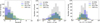 |
Fig. 1. Distributions of redshifts (left), rest-frame durations (middle), and rest-frame peak energies (right) of time-integrated spectra. |
2.1. The ‘KW trig’ sample
The sample of triggered KW bursts with known redshifts covering the range 0.07 ≲ z ≲ 5.0 from Tsvetkova et al. (2017), updated with the recent GRBs, comprises 193 events whose spectra are measured over the 20 keV–10 MeV range. Following Minaev & Pozanenko (2021), we used the updated or corrected redshifts for two GRBs from Tsvetkova et al. (2017): z = 1.9621 (Perley et al. 2017) for GRB 020819B and z ≃ 1.0 (Knust et al. 2017) for GRB 150424A. GRB 050603 was removed from the sample, as its redshift based on the alleged detection of a bright Lyman α line (Berger & Becker 2005) is highly unreliable given the deep non-detection of the host galaxy in follow-up observations (Hjorth et al. 2012). Finally, we excluded GRB 070508 from the sample, as its redshift was withdrawn upon deeper analysis (Fynbo et al. 2009). In this paper, we adopt the durations computed in the G2G3 (∼80−1200 keV) energy window, unless otherwise specified.
2.2. The ‘KW & BAT’ sample
We do not use Swift/BAT spectral data alone, as the limited spectral range of the instrument introduces bias to the spectral parameters and energetics (Sakamoto et al. 2011a). Accordingly, we adopted the sample from Tsvetkova et al. (2021) containing 167 GRBs with known redshifts (0.04 ≲ z ≲ 9.4), which were detected by KW in the waiting mode (20−1500 keV band) and triggered BAT. For this sample, following Minaev & Pozanenko (2020), we corrected the redshift of GRB 050803 from z = 0.422 to z = 4.3 (Perley et al. 2016). The afterglow spectrum of GRB 160327A is indicative of a Lyman-alpha drop at a redshift between 4.90 and 5.01, with the most probable value at z = 4.99, which we adopted as the redshift of this burst, although even lower redshifts could not be discarded for their unusually large hydrogen column densities. Due to the low S/N ratio of the spectrum, it was impossible to confirm any other absorption lines (de Ugarte Postigo et al. 2016). Following (Tsvetkova et al. 2021), we adopted the durations computed in the 25−350 keV band, unless otherwise specified.
2.3. The ‘GBM all’ and ‘GBM only’ samples
These sets of bursts comprise the GBM events with known redshifts spanning the range 0.01 ≲ z ≲ 8.2 collected from Gruber et al. (2011), Atteia et al. (2017), Minaev & Pozanenko (2020, 2021), and GCN circulars1. The GRB T90 durations and the peak energies of the time-integrated spectra were extracted either from the FERMIGBRST–Fermi GBM Burst Catalogue2 or from the GCN circulars. The ‘GBM all’ sample contains 168 events, and after removal of the overlap with the ‘KW trig’ and ‘KW & BAT’ samples, 49 of them comprise the ‘GBM only’ set. Following Minaev & Pozanenko (2021), we corrected the redshift of GRB 150101B. The value of z = 0.093, taken from Zhang et al. (2018), was based on an incorrect preliminary measurement by Castro-Tirado et al. (2015), which was later corrected in Levan et al. (2015), leading to z = 0.1343 (Fong et al. 2016). The GBM durations were computed in the 50−300 keV energy range.
3. Analysis and results
We fitted the skewed and non-skewed Gaussian and Student distributions to the data on the Ep versus T90 plane for the ‘Total’ sample in the observer and the source frames. As we followed a common approximation procedure, we have placed its description in the Appendix C, where its details along with all designations can be found. We also exploited the ‘KW trig’, ‘KW & BAT’, and ‘GBM all’ subsamples to test how the instrumental biases affect the GRB classification. The Akaike and Bayesian information criteria (IC) were used to estimate the relative performance of the models. The Δi (difference between the IC of the ith model and the minimum one within a set of models) for AIC and BIC yielded from this analysis, along with the corresponding model weights, wi, are summarised in Tables D.1, D.2, D.3, and D.4 for the rest frame and in Tables D.5, D.6, D.7, and D.8 for the observer frame at Zenodo and illustrated in Figure 2. In all the tables providing IC, the (equally) preferred models (ΔAIC or ΔBIC < 2) are marked with the red colour, while the acceptable models with 2 < ΔAIC < 4 are denoted with blue.
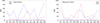 |
Fig. 2. Information criteria scores for the ‘Total’ sample. The following designations are introduced for the models: 𝒩 (𝒮𝒩) and 𝒯 (𝒮𝒯) denote the symmetric (skewed) Gaussian and Student distributions, correspondingly; the number to the left of the model provides the amount of clusters; and the number in parentheses gives the amount of free parameters of the model. The red filled area corresponds to the ΔIC < 2 area, while the blue filled area marks the 2 < ΔIC < 4 area. |
In the rest frame, the AIC gives preference to the models based on the one-component skewed distributions for all but the ‘KW & BAT’ samples while also allowing two (three) clusters with symmetric distributions for the ‘KW trig’ (‘GBM all’) subsamples. The ‘KW & BAT’ sample can be nicely fitted only by a symmetric distribution but with any number of clusters. Meanwhile, BIC only supports the one-cluster distributions. Specifically, skewed one-cluster distributions are favoured for the ‘Total’, ‘KW trig’, and ‘GBM all’ samples, and non-skewed one-cluster distributions are favoured for the ‘KW & BAT’ sample. Noticeably, the three-component models can hardly be considered as acceptable for describing the GRBs on the hardness-duration plane in the rest frame.
In the observer frame, AIC allows three-component symmetric models for all samples, while in the BIC framework, the one-component skewed models are clearly preferred over others. However, three-component skewed distribution also fits the ‘KW & BAT’ and ‘GBM all’ samples. The asymmetric one-component models are also admitted for the ‘KW & BAT’ sample, which can easily be explained by the observational biases: The detection of the short-hard GRBs is significantly suppressed by both the soft BAT energy band, whose channels prevail in number over the three KW channels, and the coarse time resolution in the waiting mode of the KW experiment.
4. Discussion
We note that, as expected, modelling the data with skewed distributions generally reduces the number of possible clusters (i.e. the distribution components) of GRBs compared to the fits with symmetric models. In addition, AIC offers a systematically wider choice of acceptable models and allows for a higher number of clusters than BIC. Remarkably, BIC yields a one-cluster model based on a skewed distribution as being best for almost all samples, both in the observer and the rest frames. The only exception is the ‘KW & BAT’ sample considered in the rest frame, for which the non-skewed one-component model is preferred. As one can see, a broader selection of models (based on AIC) is allowed for the individual subsamples than for the mixed ‘Total’ sample, where the peculiarities of different gamma-detectors with distinct sensitivities and trigger algorithms are smoothed. It is also noticeable that in many cases, similar results were obtained for the Gaussian and Student distributions in the AIC framework. This is not surprising given that when the number of degrees of freedom (the sample size) is large, the Student distribution essentially coincides with the Gaussian due to the central limit theorem. Thus, while BIC favours a single GRB cluster in both the observer and rest frames, AIC gives the preference to the three-component models in the observer frame and the one-component model in the rest frame.
4.1. Comparison with other studies
A significant number of studies consider the observer-frame burst durations and the ‘count ratio’ hardnesses to draw conclusions on the GRB classification (see, e.g., the introduction in Tarnopolski 2019a and Table 1 in Salmon et al. 2022b for a comprehensive summary of efforts to classify GRBs). Some of these studies found evidence for the third class of GRBs, while other works do not confirm this conclusion. However, several studies (e.g. Zhang et al. 2009; Li et al. 2020; Luo et al. 2023, which employed multiple criteria, including redshift) have not found it necessary to invoke the intermediate class of GRBs. Moreover, a study of almost 300 Swift/BAT bursts with known redshifts carried out using the Gaussian-mixture model and EM algorithm showed that two components suffice in both observer and rest frames based on the BIC (Yang et al. 2016).
In this work, we find that in most cases, a single cluster describes the population of GRBs with known redshifts well in their source frame on the hardness (Ep)–duration plane, which is in agreement with Tsvetkova et al. (2017). This can be explained by the blurring of the cluster boundaries in the source frame due to a wider range of the long GRB redshifts and the consequent decrease of contrast in the hardnesses and durations of short bursts compared to the long ones. The difference in the redshift range of long and short GRBs may result from selection effects, such as fainter afterglows of short bursts (Berger 2014), and the merger delay with respect to star formation (Zhang et al. 2009).
4.2. Selection effects and other distortions
The GRB observations are subject to selection effects, as the observed sample may not reflect the true underlying population. These observational distortions play a crucial role in GRBs (Turpin et al. 2016; Dainotti & Del Vecchio 2017), which are particularly affected by the Malmquist bias that favours the brightest objects against faint objects at large distances and leads to sample incompleteness. For the sample of GRBs with known redshifts, the selection effects can be divided into two categories: the instrument-specific effects caused by its trigger sensitivity to the burst prompt emission parameters and the ‘external’ biases originating from the process of GRB localisation and redshift measurement. The selection effects may affect the peak energy, the isotropic energy release, the peak, or the isotropic luminosity (see, e.g., Dainotti & Amati 2018).
The prerequisite of a reliable redshift estimate introduces an additional bias. The ‘KW trig’ and ‘GBM all’ subsamples include around 12% of short bursts compared to the 16% present in full samples of all bursts that triggered the instruments. However, the sample of BAT GRBs contains half as many short events compared to the aforementioned subsamples, both with measured redshifts and in total, and the amount is only 2% in the ‘KW & BAT’ subsample.
The GRB durations are subject to the three following redshift-driven effects. (1) Cosmological time dilation stretches durations by the factor of (1 + z). (2) A dependence of sharpness of the light curve peaks on the energy bandpass where it is collected yields narrower temporal structures in the source frame, according to the narrowing of pulses with energy (Norris et al. 1996; Fenimore et al. 1995), as any given energy window in the observer frame corresponds to a harder rest-frame band. (3) The ‘tip of the iceberg’ effect consisting of the decrease of the GRB light curve S/N ratio with larger redshifts so that the ‘wings’ of the pulses drop below the background level leaves only the brightest part of the burst as detectable (Kocevski & Petrosian 2013). The first effect can be easily corrected if the redshift is known: T90, z = T90, obs/(1 + z). The second effect, in principle, may be addressed by applying the empirical equation from Fenimore et al. (1995), which states that the duration of individual GRB emission episodes decreases with the increase of photon energy: T ∝ E−0.4. However, in practice, this property should be used with caution, as it is only valid on average. It is known that the power-law index 0.4 can vary wildly on individual GRBs (see, e.g., Borgonovo et al. 2007). The third effect is hard to correct for.
To assess the instrument-specific selection effects, we conducted an analysis of three subsamples (‘KW trig’, ‘KW & BAT’, and ‘GBM all’) separately in addition to the ‘Total’ sample. It turns out that in the rest frame, the claim of the one-component skewed distribution as the best, or at least suitable, model for the ‘Total’ sample remains valid for the ‘KW trig’ and ‘GBM all’ subsamples, leaving non-skewed models as preferable for the ‘KW & BAT’ subsample, which is the sample that is the most subject to biases. Meanwhile, in the observer frame, the best model differs depending on the IC applied. However, for each IC, the suitable model is in agreement within all subsamples and the ‘Total’ sample, despite identifying some other models as suitable as well.
To evaluate the effect of the Malmquist bias, which leads to the insecure detection of the events with energetics near the trigger threshold, we excluded 10% of the faintest bursts (based on their S/N) in each subsample and in the ‘Total’ sample, and we conducted the clustering analysis on the hardness-duration plane in the rest frame. The results, provided in Table D.9 at Zenodo, are in a good agreement with the ones claimed from the original sample and the subsamples. The results only evoke additional models based on the symmetric distributions for the ‘KW trig’ (three clusters) and ‘GBM all’ (one and two clusters) samples and retract a three-component symmetric distribution for the ‘KW & BAT’ sample.
4.3. T90 versus T50 duration
As Svinkin et al. (2019) argued that T50 is a more robust3 duration measure than T90, we studied the GRB clustering on the Ep − T50 plane in the GRB source frame applied to the ‘KW trig’ and ‘KW & BAT’ samples, as we had all the T50 durations available for them. Tables D.10 and D.11 at Zenodo along with Figure 3 provide the yielded ICs. One can see that the results are in good agreement with the ones obtained using the T90 duration. A few differences are that two-component distributions are allowed, in addition to others, in the AIC framework for the ‘KW trig’ sample.
4.4. Observer-frame versus rest-frame durations
A recent study of the GRB minimum variability timescale (Camisasca et al. 2023) showed that dependence of the GRB duration on its redshift may be weaker than expected (if present at all). This can be explained by the fact that three different effects (see Section 4.2) can reduce each other, thus decreasing the contribution of the cosmological time dilation, as also found by previous investigations (Kouveliotou et al. 1993; Golkhou & Butler 2014; Golkhou et al. 2015; Littlejohns & Butler 2014). Therefore, we examined the ‘Total’ sample on the plane of the rest-frame peak energies and the observer-frame T90 durations. The ICs, presented in Table D.12 at Zenodo, show that based on BIC, the accepted models are in good agreement with the ones yielded from the modelling of the ‘Total’ sample in both the rest and the observer frames. Nevertheless, additional multi-component models emerged in the AIC framework, but the framework tends to overfit the data.
4.5. Assessment of the uncertainties on IC
To assess the performance of the applied method, we carried out data resampling using the bootstrap (Efron 1979) and jackknife (Quenouille 1949, 1956; Tukey 1958) techniques. Applying bootstrap, we drew 100 samples from the original ‘Total’ sample, keeping the same sample size. When applying the jackknife approach, we generated two sets of new samples of 100 members each excluding 10% and 30% of the original data. Table D.13 provides the mean values and standard deviations that we used as a proxy to estimate the IC uncertainties for each set of samples. Remarkably, the adopted uncertainties are significantly higher than the thresholds on ΔIC for accepting a model as the best or, at least, suitable. The same conclusion is valid when the IC uncertainties are estimated using a set of 100 samples generated from the 1σ statistical errors of the rest-frame T90 and Ep (Table D.14 at Zenodo). Thus, the results based on the applied technique should be treated with caution.
4.6. Validation of the technique reliability
To test the robustness of the technique applied in this work, we generated a mock sample of 400 points on the hardness-duration plane, corresponding in size to the original ‘Total’ sample, and a 10 000-point mock sample from the two-dimensional two-component symmetric Gaussian distribution obtained within the previous analysis of the ‘Total’ sample. After application of the technique described in Appendix C to these mock samples, we found that the original model is firmly preferred (the separation between the IC of the models was well above the best model selection criteria, even when including the large uncertainties assessed in the previous subsection) by the larger mock sample, while the smaller sample prefers the one- and three-component non-skewed models in addition to the original one. Thus, the size of the sample under investigation is crucial to ensure the robustness of the technique.
4.7. Rest-frame versus observer-frame light curve energy bands
To address the problem of the GRB pulse narrowing with increasing energy, which results in the duration bias, one can compute durations based on the GRB time histories in two energy windows: one that is fixed in the observer frame and another that is set constant in the rest frame. However, as KW light curves are collected in three fixed energy windows and the energy band of BAT is too narrow to provide multiple energy windows for light curves, this kind of bias assessment appears to be feasible only for the GBM data. Thus, we computed T90 for the ‘GBM all’ sample based on the light curves in two energy ranges: 100−900 keV in the observer and rest frames. In the latter case, the bandpass was transformed to the 100/(1 + z)−900/(1 + z) keV interval. The durations were computed using the techniques similar to the ones described in Appendices A.1 and A.2. We excluded some relatively dim bursts from the sample, as the shift of the 50−300 keV band conventionally used by the GBM team to evaluate durations toward the harder 100−900 keV range resulted in the S/N decreasing and the consequent absence of a reliable T90 estimate for these events, thereby leaving a set of 155 GRBs under consideration. We then applied the clustering procedure to two data sets that comprise the rest-frame hardnesses and cosmological time dilation-corrected durations assessed in the two aforementioned energy bands. Figure 4 and Table D.15 at Zenodo present the comparison of the results obtained in these two cases. For both data sets, as well as for the one that includes the rest-frame T90 estimated in the standard 50−300 keV band, BIC shows a clear preference to single-component distributions. As expected, AIC offers a wider choice for the amount of clusters, and it allows a one-component distribution as a suitable model in all three cases. Remarkably, the ‘classic’ estimate of hardness, which is the ratio of counts collected in two different energy ranges, is subject to a similar bias, thus making the spectral peak energy a more robust proxy for the GRB hardness.
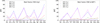 |
Fig. 3. Comparison of information criteria scores computed using the T50 and T90 durations for the ‘KW trig’ and ‘KW & BAT’ samples. The following designations are introduced for the models: 𝒩 (𝒮𝒩) and 𝒯 (𝒮𝒯) denote the symmetric (skewed) Gaussian and Student distributions, correspondingly; the number to the left of the model provides the amount of clusters; and the number in parentheses gives the amount of free parameters of the model. The red filled area corresponds to the ΔIC < 2 area, while the blue filled area marks the 2 < ΔIC < 4 area. |
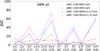 |
Fig. 4. Comparison of information criteria scores computed for the rest-frame hardness-duration distributions of 155 GRBs from the ‘GBM all’ sample. The durations were computed in the observer- and rest-frame energy windows 100 − 900 keV, which in the latter case corresponds to the |

5. Conclusions
As it has been suggested that redshift distribution may play a crucial role in GRB classification (e.g. Tarnopolski 2019a), we studied the clustering of GRBs on the hardness-duration (i.e. Ep − T90) plane in both the observer and the rest frame using data obtained by three different GRB detectors. The results obtained from the sample of 409 GRBs with known redshifts detected in a wide energy range, one of the largest to date in terms of the informational criteria, do not show evidence of a third class of GRBs in the rest frame4. In addition, the results of our study confirm the conclusions made in Tsvetkova et al. (2017) for a sample of 150 KW GRBs with known redshifts detected in the triggered mode, namely, a quite prominent boundary between the type I and type II GRBs becomes blurred when the data are transformed from the observer frame to the rest frame. The robustness of the adopted technique has an obvious dependence on the sample size, and this relationship highlights the importance of the prospective missions that are aimed at substantially increasing the number of reliable GRB redshift estimates (e.g. THESEUS Amati et al. 2018, 2021).
6. Data availability
All the tables with parameters of fits of GRB hardness-duration distributions are available in the pdf and plain text formats at Zenodo.
However, the results drawn from a sample of limited size should be treated with caution (see Section 4.6).
Acknowledgments
We thank the anonymous referee for their valuable comments and suggestions that led to an overall improvement of this work. We thank Adam Goldstein for giving clarification on the GBM duration calculation procedure. We also gratefully acknowledge discussions with Dmitry Svinkin. A.T. acknowledges support from the HERMES Pathfinder–Operazioni 2022-25-HH.0 grant. L.A. acknowledges support from INAF grant programme 2022. The work of AT and DF is supported by the basic funding program of the Ioffe Institute FFUG-2024-0002.
References
- Acuner, Z., & Ryde, F. 2018, MNRAS, 475, 1708 [NASA ADS] [CrossRef] [Google Scholar]
- Ahumada, T., Singer, L. P., Anand, S., et al. 2021, Nat. Astron., 5, 917 [NASA ADS] [CrossRef] [Google Scholar]
- Akaike, H. 1974, IEEE Trans. Autom. Control, 19, 716 [Google Scholar]
- Amati, L., O’Brien, P., Götz, D., et al. 2018, Adv. Space Res., 62, 191 [Google Scholar]
- Amati, L., O’Brien, P. T., Götz, D., et al. 2021, Exp. Astron., 52, 183 [NASA ADS] [CrossRef] [Google Scholar]
- Aptekar, R. L., Frederiks, D. D., Golenetskii, S. V., et al. 1995, Space Sci. Rev., 71, 265 [NASA ADS] [CrossRef] [Google Scholar]
- Atteia, J. L., Heussaff, V., Dezalay, J. P., et al. 2017, ApJ, 837, 119 [Google Scholar]
- Azzalini, A., & Capitanio, A. 2002, J. Roy. Stat. Soc. Ser. B: Stat. Methodol., 61, 579 [Google Scholar]
- Azzalini, A., & Capitanio, A. 2003, J. Roy. Stat. Soc. Ser. B: Stat. Methodol., 65, 367 [Google Scholar]
- Band, D., Matteson, J., Ford, L., et al. 1993, ApJ, 413, 281 [Google Scholar]
- Barthelmy, S. D., Barbier, L. M., Cummings, J. R., et al. 2005, Space Sci. Rev., 120, 143 [Google Scholar]
- Basso, R. M., Lachos, V. H., Cabral, C. R. B., & Ghosh, P. 2010, Comput. Stat. Data Anal., 54, 2926 [Google Scholar]
- Berger, E. 2014, ARA&A, 52, 43 [CrossRef] [Google Scholar]
- Berger, E., & Becker, G. 2005, GRB Coordinates Network, 3520, 1 [NASA ADS] [Google Scholar]
- Biesiada, M. 2007, JCAP, 2007, 003 [CrossRef] [Google Scholar]
- Blinnikov, S. I., Novikov, I. D., Perevodchikova, T. V., & Polnarev, A. G. 1984, Sov. Astron. Lett., 10, 177 [Google Scholar]
- Borgonovo, L., Frontera, F., Guidorzi, C., et al. 2007, A&A, 465, 765 [NASA ADS] [CrossRef] [EDP Sciences] [Google Scholar]
- Burnham, K. P., & Anderson, D. R. 2004, Soc. Meth. Res., 33, 261 [Google Scholar]
- Cabral, C. R. B., Lachos, V. H., & Prates, M. O. 2012, Comput. Stat. Data Anal., 56, 126 [Google Scholar]
- Camisasca, A. E., Guidorzi, C., Amati, L., et al. 2023, A&A, 671, A112 [NASA ADS] [CrossRef] [EDP Sciences] [Google Scholar]
- Castro-Tirado, A. J., Sanchez-Ramirez, R., Gorosabel, J., & Scarpa, R. 2015, GRB Coordinates Network, 17278, 1 [Google Scholar]
- Dainotti, M. G., & Amati, L. 2018, PASP, 130, 051001 [Google Scholar]
- Dainotti, M. G., & Del Vecchio, R. 2017, New Astron. Rev., 77, 23 [Google Scholar]
- de Ugarte Postigo, A., Horváth, I., Veres, P., et al. 2011, A&A, 525, A109 [NASA ADS] [CrossRef] [EDP Sciences] [Google Scholar]
- de Ugarte Postigo, A., Tanvir, N. R., Cano, Z., et al. 2016, GRB Coordinates Network, 19245, 1 [Google Scholar]
- Dezalay, J. P., Barat, C., Talon, R., et al. 1991, Am. Inst. Phys. Conf. Ser., 265, 304 [Google Scholar]
- Dichiara, S., Troja, E., Beniamini, P., et al. 2021, ApJ, 911, L28 [Google Scholar]
- Dimple, Misra, K., & Arun, K. G. 2023, ApJ, 949, L22 [Google Scholar]
- Dimple, Misra, K., & Arun, K. G. 2024, ApJ, 974, 55 [Google Scholar]
- Efron, B. 1979, Ann. Stat., 7, 1 [Google Scholar]
- Eichler, D., Livio, M., Piran, T., & Schramm, D. N. 1989, Nature, 340, 126 [NASA ADS] [CrossRef] [Google Scholar]
- Fenimore, E. E., in ’t Zand, J. J. M., Norris, J. P., Bonnell, J. T., & Nemiroff, R. J. 1995, ApJ, 448, L101 [NASA ADS] [CrossRef] [Google Scholar]
- Fong, W., Margutti, R., Chornock, R., et al. 2016, ApJ, 833, 151 [Google Scholar]
- Fynbo, J. P. U., Jakobsson, P., Prochaska, J. X., et al. 2009, ApJS, 185, 526 [NASA ADS] [CrossRef] [Google Scholar]
- Gehrels, N., Chincarini, G., Giommi, P., et al. 2004, ApJ, 611, 1005 [Google Scholar]
- Gillanders, J. H., Troja, E., Fryer, C. L., et al. 2023, ArXiv e-prints [arXiv:2308.00633] [Google Scholar]
- Golkhou, V. Z., & Butler, N. R. 2014, ApJ, 787, 90 [NASA ADS] [CrossRef] [Google Scholar]
- Golkhou, V. Z., Butler, N. R., & Littlejohns, O. M. 2015, ApJ, 811, 93 [NASA ADS] [CrossRef] [Google Scholar]
- Gruber, D., Greiner, J., von Kienlin, A., et al. 2011, A&A, 531, A20 [NASA ADS] [CrossRef] [EDP Sciences] [Google Scholar]
- Hjorth, J., Malesani, D., Jakobsson, P., et al. 2012, ApJ, 756, 187 [Google Scholar]
- Horváth, I. 1998, ApJ, 508, 757 [CrossRef] [Google Scholar]
- Huja, D., Mészáros, A., & Řípa, J. 2009, A&A, 504, 67 [NASA ADS] [CrossRef] [EDP Sciences] [Google Scholar]
- Jespersen, C. K., Severin, J. B., Steinhardt, C. L., et al. 2020, ApJ, 896, L20 [NASA ADS] [CrossRef] [Google Scholar]
- Kass, R. E., & Raftery, A. E. 1995, J. Am. Stat. Assoc., 90, 773 [Google Scholar]
- Knust, F., Greiner, J., van Eerten, H. J., et al. 2017, A&A, 607, A84 [NASA ADS] [CrossRef] [EDP Sciences] [Google Scholar]
- Kocevski, D., & Petrosian, V. 2013, ApJ, 765, 116 [NASA ADS] [CrossRef] [Google Scholar]
- Koen, C., & Bere, A. 2012, MNRAS, 420, 405 [NASA ADS] [CrossRef] [Google Scholar]
- Kouveliotou, C., Meegan, C. A., Fishman, G. J., et al. 1993, ApJ, 413, L101 [NASA ADS] [CrossRef] [Google Scholar]
- Kulkarni, S., & Desai, S. 2017, Ap&SS, 362, 70 [Google Scholar]
- Kwong, H. S., & Nadarajah, S. 2018, MNRAS, 473, 625 [NASA ADS] [CrossRef] [Google Scholar]
- Levan, A., Hjorth, J., Wiersema, K., & Tanvir, N. 2015, ATel, 6873, 1 [Google Scholar]
- Levan, A. J., Gompertz, B. P., Salafia, O. S., et al. 2024, Nature, 626, 737 [NASA ADS] [CrossRef] [Google Scholar]
- Li, Y., Zhang, B., & Yuan, Q. 2020, ApJ, 897, 154 [NASA ADS] [CrossRef] [Google Scholar]
- Liddle, A. R. 2007, MNRAS, 377, L74 [NASA ADS] [Google Scholar]
- Lien, A., Sakamoto, T., Barthelmy, S. D., et al. 2016, ApJ, 829, 7 [Google Scholar]
- Littlejohns, O. M., & Butler, N. R. 2014, MNRAS, 444, 3948 [NASA ADS] [CrossRef] [Google Scholar]
- Luo, J.-W., Wang, F.-F., Zhu-Ge, J.-M., et al. 2023, ApJ, 959, 44 [Google Scholar]
- MacFadyen, A. I., & Woosley, S. E. 1999, ApJ, 524, 262 [NASA ADS] [CrossRef] [Google Scholar]
- Mazets, E. P., Golenetskii, S. V., Ilinskii, V. N., et al. 1981, Ap&SS, 80, 3 [NASA ADS] [CrossRef] [Google Scholar]
- Meegan, C., Lichti, G., Bhat, P. N., et al. 2009, ApJ, 702, 791 [Google Scholar]
- Minaev, P. Y., & Pozanenko, A. S. 2020, MNRAS, 492, 1919 [NASA ADS] [CrossRef] [Google Scholar]
- Minaev, P. Y., & Pozanenko, A. S. 2021, MNRAS, 504, 926 [Google Scholar]
- Narayan, R., Paczynski, B., & Piran, T. 1992, ApJ, 395, L83 [NASA ADS] [CrossRef] [Google Scholar]
- Norris, J. P., & Bonnell, J. T. 2006, ApJ, 643, 266 [NASA ADS] [CrossRef] [Google Scholar]
- Norris, J. P., Cline, T. L., Desai, U. D., & Teegarden, B. J. 1984, Nature, 308, 434 [NASA ADS] [CrossRef] [Google Scholar]
- Norris, J. P., Nemiroff, R. J., Bonnell, J. T., et al. 1996, ApJ, 459, 393 [NASA ADS] [CrossRef] [Google Scholar]
- Paczynski, B. 1986, ApJ, 308, L43 [NASA ADS] [CrossRef] [Google Scholar]
- Paczynski, B. 1991, Acta Astron., 41, 257 [NASA ADS] [Google Scholar]
- Paczyński, B. 1998, ApJ, 494, L45 [Google Scholar]
- Perley, D. A., Tanvir, N. R., Hjorth, J., et al. 2016, ApJ, 817, 8 [Google Scholar]
- Perley, D. A., Krühler, T., Schady, P., et al. 2017, MNRAS, 465, L89 [Google Scholar]
- Prates, M. O., Lachos, V. H., & Barbosa Cabral, C. R. 2013, J. Stat. Softw., 54, 1 [Google Scholar]
- Quenouille, M. H. 1949, Ann. Math. Stat., 20, 355 [Google Scholar]
- Quenouille, M. H. 1956, Biometrika, 43, 353 [Google Scholar]
- Rastinejad, J. C., Gompertz, B. P., Levan, A. J., et al. 2022, Nature, 612, 223 [NASA ADS] [CrossRef] [Google Scholar]
- Rossi, A., Rothberg, B., Palazzi, E., et al. 2022, ApJ, 932, 1 [NASA ADS] [CrossRef] [Google Scholar]
- Sakamoto, T., Barthelmy, S. D., Barbier, L., et al. 2008, ApJS, 175, 179 [NASA ADS] [CrossRef] [Google Scholar]
- Sakamoto, T., Pal’Shin, V., Yamaoka, K., et al. 2011a, PASJ, 63, 215 [Google Scholar]
- Sakamoto, T., Barthelmy, S. D., Baumgartner, W. H., et al. 2011b, ApJS, 195, 2 [Google Scholar]
- Salmon, L., Hanlon, L., & Martin-Carrillo, A. 2022a, Galaxies, 10, 78 [Google Scholar]
- Salmon, L., Hanlon, L., & Martin-Carrillo, A. 2022b, Galaxies, 10, 77 [NASA ADS] [CrossRef] [Google Scholar]
- Scargle, J. D., Norris, J. P., Jackson, B., & Chiang, J. 2013, ApJ, 764, 167 [Google Scholar]
- Schwarz, G. 1978, Ann. Stat., 6, 461 [Google Scholar]
- Svinkin, D. S., Frederiks, D. D., Aptekar, R. L., et al. 2016, ApJS, 224, 10 [CrossRef] [Google Scholar]
- Svinkin, D. S., Aptekar, R. L., Golenetskii, S. V., et al. 2019, J. Phys. Conf. Ser., 1400, 022010 [Google Scholar]
- Tarnopolski, M. 2015, A&A, 581, A29 [NASA ADS] [CrossRef] [EDP Sciences] [Google Scholar]
- Tarnopolski, M. 2016a, MNRAS, 458, 2024 [NASA ADS] [CrossRef] [Google Scholar]
- Tarnopolski, M. 2016b, Ap&SS, 361, 125 [CrossRef] [Google Scholar]
- Tarnopolski, M. 2016c, New Astron., 46, 54 [Google Scholar]
- Tarnopolski, M. 2019a, ApJ, 870, 105 [CrossRef] [Google Scholar]
- Tarnopolski, M. 2019b, ApJ, 887, 97 [NASA ADS] [CrossRef] [Google Scholar]
- Troja, E., Fryer, C. L., O’Connor, B., et al. 2022, Nature, 612, 228 [NASA ADS] [CrossRef] [Google Scholar]
- Tsvetkova, A., Frederiks, D., Golenetskii, S., et al. 2017, ApJ, 850, 161 [NASA ADS] [CrossRef] [Google Scholar]
- Tsvetkova, A., Frederiks, D., Svinkin, D., et al. 2021, ApJ, 908, 83 [NASA ADS] [CrossRef] [Google Scholar]
- Tsvetkova, A., Svinkin, D., Karpov, S., & Frederiks, D. 2022, Universe, 8, 373 [NASA ADS] [CrossRef] [Google Scholar]
- Tukey, J. W. 1958, Ann. Math. Stat., 29, 614 [CrossRef] [Google Scholar]
- Turpin, D., Heussaff, V., Dezalay, J. P., et al. 2016, ApJ, 831, 28 [Google Scholar]
- von Kienlin, A., Meegan, C. A., Paciesas, W. S., et al. 2014, ApJS, 211, 13 [Google Scholar]
- Wagenmakers, E.-J., & Farrell, S. 2004, Psychon. Bull. Rev., 11, 192 [Google Scholar]
- Woosley, S. E. 1993, ApJ, 405, 273 [Google Scholar]
- Woosley, S. E., & Bloom, J. S. 2006, ARA&A, 44, 507 [Google Scholar]
- Yang, E. B., Zhang, Z. B., & Jiang, X. X. 2016, Ap&SS, 361, 257 [NASA ADS] [CrossRef] [Google Scholar]
- Yang, J., Ai, S., Zhang, B.-B., et al. 2022, Nature, 612, 232 [NASA ADS] [CrossRef] [Google Scholar]
- Yang, Y.-H., Troja, E., O’Connor, B., et al. 2024, Nature, 626, 742 [NASA ADS] [CrossRef] [Google Scholar]
- Zhang, B., Zhang, B.-B., Virgili, F. J., et al. 2009, ApJ, 703, 1696 [NASA ADS] [CrossRef] [Google Scholar]
- Zhang, Z.-B., Yang, E.-B., Choi, C.-S., & Chang, H.-Y. 2016, MNRAS, 462, 3243 [NASA ADS] [CrossRef] [Google Scholar]
- Zhang, Z. B., Zhang, C. T., Zhao, Y. X., et al. 2018, PASP, 130, 054202 [CrossRef] [Google Scholar]
- Zitouni, H., Guessoum, N., Azzam, W. J., & Mochkovitch, R. 2015, Ap&SS, 357, 7 [Google Scholar]
Appendix A: Instrumentation
A.1. Konus-Wind
The Konus-Wind (hereafter KW; Aptekar et al. 1995) experiment has been operating since 1994 November continuously observes the full sky by two omnidirectional NaI detectors (S1 and S2) with high temporal resolution (down to 2 ms for light curves and 64 ms for spectra) in the wide energy range of ∼10 keV−10 MeV, nominally, which is now ∼20 keV−20 MeV. The instrument has two operational modes: waiting and triggered. In the triggered mode, the light curves are recorded in three energy windows: G1 (∼13−50 keV), G2 (∼50−200 keV), and G3 (∼200−760 keV) with the time resolution varying from 2 ms to 256 ms. The detector sensitivity5 can be estimated as 1 − 2 × 10⁻⁶ erg cm−2 s−1 and 5 × 10⁻⁷ erg cm−2 s−1 in the triggered and waiting modes, correspondingly. Further details on the triggered and waiting mode data can be found in Tsvetkova et al. (2021). As for June 2024, the instrument has detected ∼ 3800 triggered GRBs.
A.2. Swift/BAT
The Neil Gehrels Swift Observatory, dedicated primarily to GRB afterglow studies, was launched on 2004 November 20 (Gehrels et al. 2004). BAT is a highly sensitive, large field-of-view (FOV; 1.4 sr for > 50% coded FOV and 2.2 sr for > 10% coded FOV) coded-aperture telescope onboard Swift that detects and localises GRBs in real time. The BAT energy range spans 14−150 keV in imaging mode. The detector sensitivity is around 1 × 10⁻⁸ erg cm−2 s−1. However, the effective limiting flux of the sample is dominated by the lower the KW waiting-mode sensitivity. Further details of the BAT instrument, including the in-orbit calibrations, can be found in Barthelmy et al. (2005) and the BAT GRB catalogues (Sakamoto et al. 2008, 2011b; Lien et al. 2016). Up to June 2024, BAT has detected ∼1600 GRBs, of which ∼430 events have measured redshifts.
A.3. Fermi/GBM
The Fermi Gamma-ray Space Observatory, which is dedicated to the study of transient gamma-ray sources, was launched in June 2008. The Gamma-ray Burst Monitor (GBM; Meegan et al. 2009) instrument onboard it observes the whole sky not occulted by the Earth (> 8 sr) covering the energy range from 8 keV to 40 MeV and is composed of 12 NaI(Tl) detectors and two bismuth-germanate (BGO) scintillation detectors. The instrument sensitivity is around 5 × 10⁻⁸ erg cm−2 s−1. More details on the design and performance of the facilities detecting GRBs may be found in Tsvetkova et al. (2022). So far, GBM has detected ∼3800 triggered GRBs.
Appendix B: Remarks on the duration computation
Despite T90, the time interval that contains 5% to 95% of the total burst count fluence, is defined unambiguously, the methodology of the computation of the total GRB duration (T100), which T90 is connected with, differs in these three samples. (1) To compute T100 durations for the triggered KW sample, a concatenation of waiting-mode and triggered-mode light curves in the ∼80–1200 keV energy range was used. The burst’s start and end times were determined at 5σ excess above background on the timescales from 2 ms to 2.944 s in the interval from T0 − 200 s to T0 + 240 s (the end of the KW triggered mode record). In some cases, the search interval was narrowed to exclude a non-GRB event overlapping with a target event. The background was approximated by a constant, using, typically, the interval from T − 1200 s to T − 200 s6, during which count rates in all energy ranges of both KW detectors are consistent with being Poisson distributed. Further details can be found in Section 4.1.1. in Tsvetkova et al. (2017). (2) The T100 durations for the ‘KW & BAT’ sample were determined using the Bayesian block decomposition (Scargle et al. 2013) of the BAT light curve collected with the 64-ms time binning in the 25–350 keV energy band. This energy band was selected as, first, being common to both instruments and, second, being less sensitive to weak precursors or soft extended tails. (3) The standard practise for the GBM T100 calculation is to generally identify, by eye, what are the pre-burst and post-burst time intervals for background assessment. After background is fit to pre- and post-burst regions, the light curve is split into 64-ms bins and each bin is fit to retrieve the deconvolved photon flux. That flux is then cumulatively added, which generates an S-shaped curve for a single-pulse GRB (see Fig 3 in von Kienlin et al. 2014). The time at which the curve deviates from the plateau indicates the start and stop times of the burst.
We compared the T90 durations of the bursts belonging to the intersection of the ‘GBM all’ and two other samples (the ‘KW trig’ and ‘KW & BAT’ samples obviously do not overlap). Overall, the median value of the T90 ratios is around unity, despite for some outliers, especially for the weak bursts, the discrepancy between the durations may reach 1.5 orders of magnitude.
Appendix C: Methods
In this Section, we follow the notations in Tarnopolski (2019a).
C.1. Distributions
We approximated the data on the hardness-duration plane with the Normal and Student distributions, both skewed and non-skewed. The Student-t distribution is symmetric, similarly to the normal distribution, but has a wider spread and a more slender shape. For each of the four distributions, we fitted the data with a mixture of one to three components, therefore implying one, two, or three clusters of GRBs. The probability density function (PDF) of a mixture of n components with individual PDFs fi(x, θ(i)) is
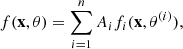
where Ai are the weights:  , and
, and  are the distribution parameters.
The k-dimensional Gaussian (Normal) distribution is described by the PDF:
![$$ f^{(N)}_k(\mathbf x, \mu , \Sigma ) = \frac{1}{\sqrt{(2 \pi )^k |\Sigma |}} \exp \left[-\frac{1}{2}(\mathbf x - \mathbf \mu )^\top \Sigma ^{-1} (\mathbf x - \mathbf \mu )\right], $$](/articles/aa/full_html/2025/06/aa52673-24/aa52673-24-eq5.gif)
where μ is the location vector, which in the case of a non-skewed distribution is also the mean, Σ is the covariance matrix, and |Σ|=detΣ. A mixture of n components has p = 6n − 1 free parameters for k = 2.
The multivariate skew-normal distribution (Azzalini & Capitanio 2002; Prates et al. 2013) is defined by

where Φ is the Cumulative Distribution Function (CDF) of a univariate standard normal distribution, and λ is the skewness parameter vector. Indeed, the skewed Normal distribution reduces to the Gaussian one at λ = 0. The mean and the covariance of the skewed-Normal distribution are given by 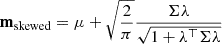 and Σskewed = Σ − (m − μ)(m − μ)⊤, where ⊤ denotes the transpose of a matrix, correspondingly. For this distribution, the number of free parameters defining mixture of n components is p = 8n − 1.
The multivariate Student distribution (Basso et al. 2010; Cabral et al. 2012; Prates et al. 2013) with ν degrees of freedom (d.o.f.) is described by
where Γ is the gamma function, μ is the mean of the distribution for ν > 1, while the covariance matrix (for ν > 2) is  . The Student distribution approaches the Gaussian in the limit of ν → ∞. A mixture of n components has p = 6n free parameters.
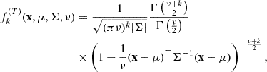
The multivariate skew-Student distribution (Cabral et al. 2012; Prates et al. 2013) is defined as
where Tν + k is the CDF of the standard univariate Student distribution with ν + k d.o.f., and λ defines the skewness parameter vector. The skewed Student distribution reduces to the non-skewed one when λ = 0, meanwhile it approaches the skewed Normal distribution in the limit of ν → ∞. The mean for ν > 1 is given by mskewed = μ + ωξ, while its covariance for ν > 2 is  , where
 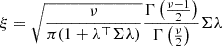 and ω = diag(Σ11, …, Σkk)1/2 (Azzalini & Capitanio 2003). A mixture of n components is described by p = 8n free parameters and has a non-zero skewness unless λ = 0 for n > 3.
C.2. Model comparison using Information Criteria
For a multidimensional distribution with a PDF f = f(x, θ), possibly a mixture, where θ = θii = 1p is a set of p parameters, the log-likelihood function is
where {xi}i = 1N are N data points from the sample to which a distribution is fitted.
To fit a model to the data, we searched the set of parameters  that yields the highest value of likelihood (ℒp, max) using the package mixsmsn7 (Prates et al. 2013) developed for the R language8. This package implements routines for maximum likelihood estimation via an expectation maximisation EM-type algorithm (Basso et al. 2010; Cabral et al. 2012). The initial values for the distribution parameters were obtained using a combination of the R function kmeans and the method of moments.
For both nested and non-nested models, the Akaike (AIC) and Bayesian (BIC) information criteria (IC) may be applied (Akaike 1974; Schwarz 1978; Burnham & Anderson 2004; Biesiada 2007; Liddle 2007; Tarnopolski 2016c,a) to estimate of the model performance. They are defined as

and

The favoured model is selected based on the minimum of AIC or BIC. Both IC comprise two competing terms: the first measuring the model complexity (number of free parameters) and the second measuring the goodness of fit (or more precisely, its lack). The IC penalise the use of an excessive number of parameters: the preference is given to the models with fewer parameters, as long as the others do not yield an essentially better fit. For BIC, the penalisation term is greater than the corresponding term for the AIC: plnN > 2p, for N ≥ 8. Consequently, the BIC provides much stricter penalisation of additional parameters than AIC, especially for large samples. Hence, BIC tends to underfit the data giving preference to an excessively simple model, while AIC is biased towards overfitting, i.e. favouring models with excessive parameters. This may lead to selection of different best-fit models using two criteria. Essentially, these two IC answer different questions: AIC selects a model that better describes the data (the model being a real description of the data is never considered), while BIC intends finding the true model among the set of candidates (Tarnopolski 2019a). Tarnopolski (2019b) found that BIC is more accurate then AIC when applied to the non-skewed distributions, while both criteria are consistent with each other for the skewed distributions.
The suitable models of fit can be assessed using the difference, Δi = AICi − AICmin, where AICmin is the minimum value of AIC over the set of 12 models, i.e. four distributions with different number of components, ranging from one to three. If Δi < 2, then there is strong support for the i-th model (or the evidence against it is worth only a small mention), and it is highly probable that this model is a proper description of the data. If 2 < Δi < 4, then there is significant support for the i-th model. When 4 < Δi < 7, there is considerably less support, and models with Δi > 10 have essentially no support (Burnham & Anderson 2004; Biesiada 2007). It is worth noting that when two models with similar ℒmax are considered, the Δi only depends on the number of parameters due to the 2p term. Thus, Δi/(2Δp) < 1, where Δp is the difference in the model parameter number, evidences that the relative improvement is owing to the fit improvement, not an increase of the number of parameters only.
Similarly for BIC, Δi = BICi − BICmin, where BICmin corresponds to the minimum BIC value within the set of 12 models, defines the degree of preference of the i-th model: if Δi < 2, then there is substantial support for the i-th model. For 2 < Δi < 6, there is positive evidence against the i-th model. If 6 < Δi < 10, the evidence is strong, and models with Δi > 10 yield very strong evidence against the i-th model, i.e. essentially no support (Kass & Raftery 1995).
Additionally, we estimated the Akaike weights, which can be directly interpreted as conditional probabilities for each model (see Burnham & Anderson 2004; Wagenmakers & Farrell 2004 and references therein):
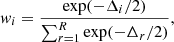
where the denominator represents a sum over all models. The Akaike weight can be interpreted as the probability of the model to be the best given the data and the set of models. Thus, the strength of evidence in favour of one model relative to another can be assessed using the ratio of their weights wi/wj or normalised probability wi/(wi + wj). Similar values for BIC, called the ‘Schwarz’ weights, can be obtained by replacing the AIC values by the BIC values in the equation for the Akaike weights.
All Tables
All Figures
|
Fig. 1. Distributions of redshifts (left), rest-frame durations (middle), and rest-frame peak energies (right) of time-integrated spectra. |
| In the text | |
|
Fig. 2. Information criteria scores for the ‘Total’ sample. The following designations are introduced for the models: 𝒩 (𝒮𝒩) and 𝒯 (𝒮𝒯) denote the symmetric (skewed) Gaussian and Student distributions, correspondingly; the number to the left of the model provides the amount of clusters; and the number in parentheses gives the amount of free parameters of the model. The red filled area corresponds to the ΔIC < 2 area, while the blue filled area marks the 2 < ΔIC < 4 area. |
| In the text | |
|
Fig. 3. Comparison of information criteria scores computed using the T50 and T90 durations for the ‘KW trig’ and ‘KW & BAT’ samples. The following designations are introduced for the models: 𝒩 (𝒮𝒩) and 𝒯 (𝒮𝒯) denote the symmetric (skewed) Gaussian and Student distributions, correspondingly; the number to the left of the model provides the amount of clusters; and the number in parentheses gives the amount of free parameters of the model. The red filled area corresponds to the ΔIC < 2 area, while the blue filled area marks the 2 < ΔIC < 4 area. |
| In the text | |
|
Fig. 4. Comparison of information criteria scores computed for the rest-frame hardness-duration distributions of 155 GRBs from the ‘GBM all’ sample. The durations were computed in the observer- and rest-frame energy windows 100 − 900 keV, which in the latter case corresponds to the |
| In the text | |
Current usage metrics show cumulative count of Article Views (full-text article views including HTML views, PDF and ePub downloads, according to the available data) and Abstracts Views on Vision4Press platform.
Data correspond to usage on the plateform after 2015. The current usage metrics is available 48-96 hours after online publication and is updated daily on week days.
Initial download of the metrics may take a while.