| Issue |
A&A
Volume 693, January 2025
|
|
|---|---|---|
| Article Number | A156 | |
| Number of page(s) | 15 | |
| Section | Astrophysical processes | |
| DOI | https://doi.org/10.1051/0004-6361/202451776 | |
| Published online | 14 January 2025 | |
Gamma-ray burst spectral-luminosity correlations in the synchrotron scenario
1
Gran Sasso Science Institute (GSSI), Via F. Crispi 7, 67100 L’Aquila, Italy
2
INFN–Laboratori Nazionali del Gran Sasso, I-67100 L’Aquila (AQ), Italy
⋆ Corresponding author; This email address is being protected from spambots. You need JavaScript enabled to view it.
Received:
2
August
2024
Accepted:
15
November
2024
Abstract
Context. For over two decades, gamma-ray burst (GRB) prompt emission spectra were modeled with smoothly broken power laws (Band function), and a positive and tight correlation between the spectral rest-frame peak energy, Ep,z, and the total isotropic-equivalent luminosity, Liso, was found, constituting the so-called Yonetoku relation. However, more recent studies show that many prompt emission spectra are well described by the synchrotron radiation model, and hence significantly deviate from the Band function.
Aims. In this work, we test the impact of a more refined spectral model such as an idealized synchrotron spectrum from nonthermal electrons on the Yonetoku relation and its connection with physical parameters.
Methods. We selected GRBs with measured redshift observed by Fermi/GBM together with high-energy observations (> 30 MeV), and performed a spectral analysis, dividing them in two samples: the single-bin sample, using the light curve peak spectrum of each GRB, and the multiple-bin sample, for which we explored the whole duration of 13 bright bursts with time-resolved spectral analysis.
Results. We observed that the Ep,z of synchrotron spectra in a fast-cooling regime (νm/νc ≫ 1) is generally larger than the one provided by the Band function. For this reason, we do not find any Ep,z−Liso correlation in our samples except for the GRBs in an intermediate-cooling regime (1< νm/νc< 3); namely, where peak and break energies are very close. We instead find in both our samples a new tight correlation between the rest-frame cooling frequency, νc, z, and Liso: νc,z ∝ Liso(0.53±0.06).
Conclusions. These results suggest that, assuming that prompt emission spectra are produced by synchrotron radiation, the physical relation is between νc, z and Liso. The fit of the Band function to an intrinsic synchrotron spectrum returns peak energy values of Ep,zBand ∼ νc,z. This may explain why the systematic interpretation of prompt spectra through the Band function returns the Ep, z − Liso relation.
Key words: astroparticle physics / radiation mechanisms: non-thermal / gamma-ray burst: general / gamma rays: general
© The Authors 2025
 Open Access article, published by EDP Sciences, under the terms of the Creative Commons Attribution License (https://creativecommons.org/licenses/by/4.0), which permits unrestricted use, distribution, and reproduction in any medium, provided the original work is properly cited.
This article is published in open access under the Subscribe to Open model. This email address is being protected from spambots. You need JavaScript enabled to view it. to support open access publication.
1. Introduction
Cosmic explosions triggered by collapses of massive stars (Woosley 1993; Woosley & Bloom 2006) or binary neutron star mergers (Eichler et al. 1989; Narayan et al. 1992; Berger 2014; Abbott et al. 2017) produce gamma-ray bursts (GRBs), the most luminous transient phenomena in the Universe (Paczynski 1986). Thanks to several decades of observations, GRBs have been revealed to be associated with highly collimated ultra-relativistic jets launched in the aftermath of their progenitor’s explosion (see Salafia & Ghirlanda 2022, for a review).
The very fast prompt emission variability (e.g., Bhat et al. 2012) clearly suggests an emission site internal to the jet (Sari & Piran 1997). A natural explanation for the jet kinetic energy dissipation is through internal shocks (Rees & Meszaros 1994). However, sub-photospheric dissipation (Rees & Mészáros 2005; Pe’er 2008) or magnetic reconnection processes (Drenkhahn & Spruit 2002; Zhang & Yan 2011) are equally able to explain the GRB radiative output. The early emission observed soon after the explosion, during the so-called prompt emission phase, shows a broad and peaked spectral energy density (SED) that is possibly associated with nonthermal radiative processes. Historically, prompt emission spectra were modeled by the phenomenological Band function (Band et al. 1993); namely, two power laws smoothly connected around a peak at energy Ep. The systematic fit of this model to large samples of GRB spectra revealed that in some cases the low-energy photon index, α, was consistent with the one predicted by synchrotron emission in a fast-cooling regime, whereas some other GRBs exhibited very hard α, pointing toward quasi-thermal processes (Ghisellini & Celotti 1999; Lazzati et al. 2000; Mészáros & Rees 2000). The vast majority of the GRBs showed average behavior, with spectra that were too hard to be produced by synchrotron processes, but too soft to indicate thermal origins (Preece et al. 1998; Kaneko et al. 2006; Gruber et al. 2014).
This tension was partially mitigated when more complex models were employed and low-energy spectral breaks were identified in some GRB spectra at energies, Eb. It was shown that a single synchrotron spectrum in a marginally fast-cooling regime (Oganesyan et al. 2017, 2018; Ravasio et al. 2019), a slow-cooling regime (Zhang et al. 2009; Burgess et al. 2020), or even synchrotron self-absorption (Lloyd & Petrosian 2000; Lloyd-Ronning & Petrosian 2002) are able to account for the entire prompt emission spectrum, from the optical (Oganesyan et al. 2019) up to the GeV band (Macera et al., in prep.). Despite the synchrotron model seeming to be a viable explanation for most of the considered spectra, GRBs show diverse spectral and temporal behaviors, preventing a convincing unified interpretation.
A feature that appears to be shared among GRBs is that their prompt spectrum is harder when the GRB is brighter and more energetic. In fact, many sources show that the rest-frame spectral peak energy, Ep, z, is positively and tightly correlated with the isotropic-equivalent energy, Eiso (Amati et al. 2002), and luminosity, Liso (Yonetoku et al. 2004). These two relations span several decades in both energies and luminosities, and despite being affected by selection and observational biases (Band & Preece 2005; Nakar & Piran 2005; Butler et al. 2007; Shahmoradi & Nemiroff 2011), they seem to hold for most of the GRB class (Ghirlanda et al. 2008; Nava et al. 2008), and also at different redshifts (Nava et al. 2012).
In particular, the Ep, z − Eiso relation (better known as the “Amati relation”) was initially found for long GRBs, with durations of T90 > 2 s. Short GRBs (T90 < 2 s) exhibit a similar trend but occupy a parallel track in the Ep, z − Eiso plane (Ghirlanda et al. 2009), showing a systematically lower Eiso for the same Ep, z. On the other hand, both long and short GRBs follow the same Ep, z − Liso relation (better known as the “Yonetoku relation”, Yonetoku et al. 2010). After their first discoveries, many outliers to these relations were found; however, both the Amati and Yonetoku relations still hold when multiple time bins from the same bright GRB are considered through time-resolved spectral fits (Ghirlanda et al. 2010, 2011a,b).
At odds with the Amati relation, which is obtained comparing quantities averaged across the whole burst duration, the Yonetoku relation is found considering Liso (but also Ep,z, e.g., Tsvetkova et al. 2017) estimates only during the brightest pulse; in other words, at the peak of the light curve. This makes the Yonetoku relation inherently connected with the physics taking place in single GRB pulses, and it appears particularly well suited for inquiring into prompt emission physics in depth.
For more than two decades, the observations carried out by gamma-ray instruments such as the Burst Alert Telescope (BAT: 15–150 keV) on board the Neil Gehrels Swift Observatory (Swift), the Gamma-ray Burst Monitor (GBM; 8 keV–40 MeV) on board the Fermi satellite, and Konus-Wind (KW, ∼20 keV–20 MeV) have further corroborated the validity of these correlations (e.g., Nava et al. 2012; Tsvetkova et al. 2017; Minaev & Pozanenko 2020; Wang et al. 2024). Despite all these findings pointing toward a possible common emission mechanism occurring in GRB central engines, a clear physical interpretation of these correlations is still missing (see Parsotan & Ito 2022, for a review).
In this work, we carry out spectral fits of GRB samples detected by Fermi/GBM using not only the phenomenological Band function, but also a physical synchrotron model. Our goals are (i) to test whether using a physical model allows one to derive the Ep,z−Liso (Yonetoku) relation and (ii) to explore any possible connection between the Yonetoku relation and physical synchrotron parameters such as the characteristic minimum frequency, νm, and the cooling frequency, νc.
The paper is organized as follows. In Sect. 2, we describe the sample selection and the spectral modeling; in Sect. 3, we show the results of the spectral fit to the whole sample of GRBs (single-bin sample) and the time-resolved analysis of a subsample of bright GRBs (multiple-bin sample); in Sect. 4, we discuss the results; and finally, in Sect. 5, we summarize the conclusions. Throughout the paper, we assume standard cosmology with h = ΩΛ = 0.7 and Ωm = 0.3. If not stated differently, errors are reported at a 68% confidence level. As a convention, the subscript z refers to rest-frame parameters.
2. Methods
2.1. Sample selection
We analyzed GRBs observed by the Fermi satellite before September 2023. We selected the GRBs with a firm redshift estimate, provided by the MPE GRB online catalog1. We considered only the GRBs that are bright enough during their main pulse to perform a robust spectral analysis in that temporal bin. Specifically, we included in our sample only the GRBs whose 1s peak photon flux in the energy range 50–300 keV is P ≥ 3.5 photons s−1 cm−2, which corresponds to nearly seven times the flux sensitivity of Fermi/GBM. We excluded GRB221009A, GRB230307A, and GRB130427A, the three brightest GRBs, since their emission during the peak are affected by pileup effects and their GBM data cannot be used for spectral analysis.
This leads to a total sample of 74 GRBs, with a spectroscopic redshift estimate for 70 of them. Three GRBs (GRB100816A, GRB200826A, and GRB211211A) have a redshift estimate through host galaxy association, while one GRB (GRB200829A) has a photometric redshift estimate.
2.2. Data reduction
We downloaded the Fermi/GBM data (8 keV–40 MeV) of all the 74 GRBs in our sample from the Fermi GBM Burst catalog2, and performed a standard data reduction using the Fermi science tool GTBURST3. In particular, we considered data from the two sodium iodide (NaI, 8–900 keV) and one bismuth germanate (BGO, 0.3–40 MeV) detectors with best observational conditions (i.e., lowest viewing angles). In three GRBs (GRB121128A, GRB131231A, and GRB140508A), the second best NaI was exhibiting artefacts in the low-energy data (< 30 keV), leading to spectral deviations with respect to the best NaI. For this reason, for these three GRBs we considered the best and third-best NaI, together with the best BGO detector.
The background analysis was performed through GTBURST by using, whenever the polynomial fit was converging, the background intervals reported by Fermi collaboration (von Kienlin et al. 2020). In case this selection was leading to a non-convergent background polynomial fit, larger custom background intervals were selected.
We selected the source interval to coincide with the peak of the GRB light curve. The time bin is the one reported in the bcat file, a file containing basic burst parameters provided by Fermi collaboration for every GRB. The width of the time bin is 1.064 s for long GRBs (T90 > 2 s) and 256 ms for short GRBs (T90 < 2 s), in order to pinpoint their particularly short peak phase. The outputs of the data reduction are the source, background, and weighted response spectral files that are used for the spectral analysis through the Heasarc package XSPEC4 (Arnaud 1996).
The addition of high-energy (> 30 MeV) data to the prompt emission proved to be crucial in determining spectral parameters that would otherwise be inaccessible or difficult to constrain. For this reason, we decided to include in our dataset Large Area Telescope (LAT) Low Energy (LLE, 30–100 MeV) data whenever available. We retrieved the data from the Fermi LAT Low-Energy Events Catalog5. The LLE data were reduced using the same tools employed in the Fermi/GBM analysis, selecting the source in the same time bin in order to perform a simultaneous joint time-resolved analysis during the brightest peak of the emission. In our current sample, only 22 GRB have available LLE data during their peak. For those GRBs, we produced spectral files similarly to the GBM ones.
2.3. Spectral fit routine
After the data reduction, we modeled the spectra in our sample. For the fitting process, we used PYXSPEC6, the Python interface to the XSPEC spectral-fitting program. We implemented the Python-based software Bayesian X-ray analysis (BXA, Buchner 2016), which allows for Bayesian parameter estimation and model comparison through nested-sampling algorithms in PYXSPEC.
We ignored the energy channels outside 8–900 keV for the NaI detectors, as well as the 30–40 keV band in order to avoid the iodine K-edge line at 33.17 keV (Meegan et al. 2009). We selected the energy range 300 keV–40 MeV and 30–100 MeV for BGO and LLE data, respectively. For each dataset, consisting of GBM and LLE data (when available), we tested two models: the phenomenological Band function (grbm in XSPEC notation, Band et al. 1993) and an idealized physical synchrotron model. We included the presence of a cross-calibration constant, constant in XSPEC notation, allowing for a 30% variation for each dataset. We applied Poisson-Gaussian statistics (pgstat) to GBM data and Cash statistics (cstat) to LLE data. For each model, we measured the logarithm of the 10 keV–10 MeV bolometric flux in the source rest frame log F using the convolutional model cflux in XSPEC.
Moreover, in two GRBs (GRB090902B and GRB190114C) the prompt spectrum exhibits in NaI data a power law component (Abdo et al. 2009; Ajello et al. 2020; Ursi et al. 2020) in addition to the main emission one, also at low energies. Therefore, we added a power law in both the Band and synchrotron models, powerlaw in XSPEC notation. In these two cases, we computed the flux of the main component only (Band or synchrotron), since the physical nature of this additional power law was already discussed in the literature and it is outside the scope of this work.
For the synchrotron case, we used the same table model presented in Oganesyan et al. (2019). Synchrotron spectra were produced by a population of nonthermal electrons injected as a power law, dNe/dγ ∝ γ−p, with a characteristic minimum Lorentz factor, γm. The final spectrum was obtained by convolving the single electron spectrum with the electron population distribution after the particles cooled through synchrotron losses down to the cooling Lorentz factor, γc. Table spectra were produced by varying log(γm/γc) between –1 and 2, allowing for both fast (γm > γc) and slow (γm < γc) cooling regimes, and by varying p between 2 and 5 and the normalization, NSync, between 0 and 1020 (in cgs units). However, this table model assumes a constant cooling frequency, νc = 1 keV. To let this parameter vary, we multiplied the table model with the XSPEX convolutional model zmshift, which shifts the spectrum along the energy axes. The resulting photon spectrum depends on four parameters: the ratio between the Lorentz factors, γm/γc, the power law slope, p, of the injected electron distribution, the spectral shift parameter, zshift (univocally linked with the observed cooling frequency, νc), and the normalization, NSync.
2.4. Parameter estimation, model comparison, and goodness-of-fit
For each free parameter of the two models, we defined broad and uninformative priors (Table 1). The analysis returns posteriors of the parameters fit to our dataset together with the Bayesian evidence.
Free parameters and flat uninformative priors used for the spectral fit.
Being interested in physical parameters too, we derived them from the inferred ones. In the case of the Band model, we evaluated the rest frame peak energy defined as 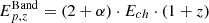 , where α is the low-energy photon index and Ech is the Band characteristic energy.
In the case of the synchrotron model, we defined the rest-frame synchrotron frequency associated with γc as νc, z = (1 + z)/(1 + zshift) and with γm as νm, z = νc, z ⋅ (γm/γc)2 and the rest frame peak energy as 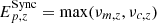 . Here, zshift is the spectral shift parameter.
In both cases, we inferred the logarithm of the 10 keV – 10 MeV rest frame flux, log F, from which we computed the flux, F = 10log F, and the total isotropic-equivalent luminosity, Liso = 4πDL2(z)⋅F, where DL(z) is the luminosity distance from the burst. For each relevant parameter, we defined the best-fit value as the median on the posterior distribution, and lower and upper errors were derived from the 16th and 84th percentile of the posterior distribution, respectively. To ensure the good convergence of the fit, we modified the prior of the cooling frequency for GRB170607A between νc ∈ (8, 500) keV; that is, zshift ∈ ( − 0.998, −0.8).
From the Bayesian fit of both models to each GRB dataset, we get the Bayesian evidence, log Z. This provides a tool with which to compare which model better describes the data. In fact, the model that has substantially larger evidence is the best-fit model. To assess this, we defined the Bayes factor for these two models as log B = log(ZSync/ZBand), and we set the threshold to 0.5 according to Jeffrey’s scale (Kass & Raftery 1995). If |log B|> 0.5, we can identify a best-fit model, which is the synchrotron one if log B > 0 or the Band function if log B < 0. If |log B|< 0.5, the Bayesian evidence of one model is not enough to statistically exclude the other.
In addition, we aim to establish whether or not the synchrotron model provides a good fit to the data. To do so, we performed posterior predictive checks (PPCs) for each synchrotron fit to our sample. By fitting a given model to a dataset, the best-fit model is the realization that maximizes the relative likelihood, and therefore returns the smallest statistics. To assess whether that model realization is a good fit to the data, we simulated 1000 fake spectra out of the best-fit model, using the XSPEC command fakeit. We estimated, for each fake spectrum, the likelihood of the best-fit model out of the fake spectrum dataset.
By repeating this computation for all the 1000 fake spectra, we can define a (Gaussian-like) probability density function relative to the statistics distribution. We measured the goodness-of-fit through a comparison of the simulated statistics distribution and the measured likelihood value. Specifically, we computed the p value of the real statistics on the simulated distribution, and we considered it a good fit if p > 0.05. We defined the p value as the integral of the simulated statistics probability density function between the best-fit statistics value and +∞ or −∞, depending on whether the measured statistics is greater or lower than the maximum of the distribution, respectively.
2.5. Linear fit routine
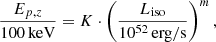
To investigate the Yonetoku relation, we fit the following power law relation to the data of our samples:
 (1)
(1)
where m and K are the power law slope and the normalization, respectively. More practically, we used the logarithmic form of Eq. (1) in order to perform a linear fit:
 (2)
(2)
We normalized both Ep,z and Liso in order to perform the linear fit closer to the data barycenter, providing better m and K estimates. Values and 1σ errors for log Ep, z and log Liso were derived directly from Ep,z and Liso parameter distributions, respectively.
We performed the fit using a Bayesian approach. We defined a likelihood that assumes Gaussian parameter distributions for both log Ep,z and log Liso and takes into account errors on both parameters with the addition of an intrinsic Gaussian noise term, σsc (D’Agostini 2005):
![Mathematical equation: $$ \begin{aligned}&{-}2 \ln \mathcal{L} \left( m, K, \sigma _{sc}\ |\ \{ x_i,\ \sigma _{x_i},\ { y}_i,\ \sigma _{{ y}_i} \}\right) \nonumber \\&= \sum _{i = 0}^N \left[ \ln \left( \sigma ^2_{sc} + \sigma ^2_{{ y}_i} + m^2 \sigma ^2_{x_i} \right) + \dfrac{({ y}_i - m(x_i - 52) - \log K+2)^2}{(\sigma ^2_{sc} + \sigma ^2_{{ y}_i} + m^2 \sigma ^2_{x_i} )} \right], \end{aligned} $$](/articles/aa/full_html/2025/01/aa51776-24/aa51776-24-eq7.gif) (3)
(3)
where N is the number of GRBs in a given sample, (xi, σxi) are log Liso mean and standard deviation relative to the i-th GRB, and (yi, σyi) are log Ep,z mean and standard deviation relative to the i-th GRB, respectively. With this approach, together with m and K, we estimated the intrinsic scatter, σsc, which constitutes a new free parameter.
Given the shape of the log Liso parameter distribution derived from the spectral fit, we note that the hypothesis of a Gaussian distribution constitutes a good approximation. For this reason, we defined σxi as the quadrature sum of its upper and lower errors. On the other hand, the shapes of log Ep,z parameter distributions are asymmetric and deviate from a classic normal distribution. To account for this inconsistency, we still approximated log Ep,z as a Gaussian, but we considered σyi to be equal to the log Ep,z upper or lower error if the data point of the i-th GRB was above or below the best-fit line, respectively.
We adopted uniform priors for the three parameter, spanning the ranges m ∈ (0, 5), K ∈ (0.01, 100), and σsc ∈ (0, 100). We sampled the posterior probability density with a Markov chain Monte Carlo approach using the emcee Python package (Foreman-Mackey et al. 2013), employing Nwalk = 32 walkers. We initialized the walkers in a small three-dimensional ball around a point in our parameter space, (m, K, σsc) = (0.5, 1.8, 10), and we performed Niter = 5000 iterations, for a total of Niter × Nwalk = 160 000 samples.
3. Results
The main results of the spectral analysis fit to our single-bin sample are shown in Tables A.1 and A.2. From the Bayes factor comparison, we see that 21 GRBs are best fit by the synchrotron model and 40 GRBs are best fit by the Band model, while the two GRBs with a second component during the prompt emission peak prefer a Band model together with a power law. For 11 GRBs, the Bayes factor modulus, |log B|, is not large enough to prefer one model over the other.
However, the comparison between Band and the synchrotron models is not straightforward. Band is a phenomenological model, and it is able to accommodate a variety of spectra by providing measures of photon indices and peak energy. On the other hand, the synchrotron model hinders many physical assumptions, providing precious insights into the nature of the emission, but still having less freedom in describing an observed spectrum.
Despite the Band function being the best-fit model for most of the GRBs in our sample, we notice that the synchrotron model provides a good fit to the data in the majority of the cases. For this reason, we split the sample in two groups: the synchrotron sample (with 58 GRBs out of 74, Table A.1) and the complementary Band sample (with 16 GRBs out of 74, Table A.2). The latter includes all the GRBs that meet at least one of the following conditions: (1.) the synchrotron model provides a good fit of the data according to the PPC criterium; (2.) the best-fit model is the synchrotron one; and (3.) the Bayes factor is not able to prefer one model to the other one. For these GRBs, we report parameter estimates obtained from the synchrotron fit.
Interestingly, all of the GRBs in this sample are in a fast-cooling regime (νm/νc > 1); therefore, in Table A.1 we report Liso, the peak energy, Ep,z = νm, z and the cooling frequency, νc, z, both in the rest-frame. On the other hand, the former sample includes all the GRBs where the synchrotron model does not provide a good fit to the data, and therefore we report parameter estimates obtained from the Band model fit.
In the synchrotron subsample, all the spectra are well fit by the synchrotron model according to the PPC criterium, except for three GRBs: GRB131231A, GRB150517A, and GRB211211A. For the first two GRBs, p − value < 0.5 because the best-fit statistics is particularly smaller than the average simulated statistics; that is, it has a significantly larger likelihood. In the case of GRB211211A, the Bayes factor prefers the synchrotron model despite the very large statistics compared to the simulated ones. In our synchrotron analysis, we get a comparable statistics with respect to the one reported by Gompertz et al. (2023) fitting a double smoothly broken power law function to the peak spectrum of this burst. Because of the model comparison, the results driven by analyzing the single-bin synchrotron subsample are valid under the assumption of synchrotron emission producing the prompt emission spectra.
3.1. Ep,z−Liso relation
We first tested the Ep,z−Liso relation obtained from the analysis of the whole sample. We computed the Spearman’s rank correlation coefficient, ρ, and its associated chance probability, Pchance. We report the results in Table 2, together with the ones of the linear fit. In Fig. 1 (left panel), we show that the data are scattered around the best-fit line, suggesting the absence of any correlation between Liso and Ep,z (ρ ∼ 0.5). In addition, the slope we obtain deviates from the one expected in the Yonetoku relation.
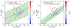 |
Fig. 1. Yonetoku relation obtained from the single-bin sample. Black stars represent GRBs from the Band subsample, while colored dots represent GRBs from the synchrotron subsample. The color scale is associated with the frequency ratio, νm/νc, derived from the synchrotron fit. We fit a power law to the whole single-bin sample (left-hand panel) and to the GRBs in the synchrotron subsample in an intermediate cooling regime (right-hand panel). The straight black line represents the best-fit line from the linear fit, and the green-shaded area the relative 3σ scatter region. For comparison, the dashed black line represents the best-fit line from Yonetoku et al. (2004). |
Results of the statistical analysis on the Ep, z − Liso and νc, z − Liso relations.
Nonetheless, we observe that GRBs with different frequency ratios, νm/νc, populate the Ep,z−Liso plane differently. In fact, GRBs with a high ratio (i.e., in a fast-cooling regime, νm/νc ≳ 10) tend to deviate from the Yonetoku relation, whereas GRBs with a lower ratio (i.e., in an intermediate-cooling regime, νm/νc ≲ 3) tend to cluster along the Yonetoku relation.
By restricting the synchrotron sample to the GRBs in the intermediate-cooling regime (1< νm/νc< 3) and fitting the relation, we find that the data points are tightly correlated, and the linear fit returns values similar to the ones obtained in Yonetoku et al. (2004) (Fig. 1, right panel). The results of this linear fit are also shown in Table 2.
3.2. A physical relation: νc, z − Liso
The Ep,z−Liso analysis previously discussed shows that, when the physical synchrotron model is used, the Yonetoku relation does not hold for the whole sample, but for only a subset of GRBs that show a synchrotron spectrum where 1< νm/νc< 3 (Fig. 1, left panel). This constitutes an important connection between the Yonetoku relation and a physical parameter; namely, the ratio between the rest-frame cooling frequency, νc, z, and the minimum frequency, νm, z. In particular, the GRBs exhibiting a relation between their Ep,z and Liso are the ones whose spectral break energy is particularly close to their peak energy.
Therefore, we tested the possibility of having a correlation between the break energy, namely the cooling frequency, νc, z, and the isotropic-equivalent luminosity, Liso. We employed the same methodology used to investigate the Ep,z−Liso relation, but applied to the synchrotron subsample of the single-bin sample (Table A.1).
We find that all of the GRBs in the synchrotron subsample, regardless of their νm/νc, show a tight νc, z − Liso correlation (Fig. 2). A Spearman’s rank correlation test returns a coefficient of ρ = 0.81 with Pchance = 1.91 × 10⁻¹⁴. The slope of the power law is consistent with both the one expected from the Yonetoku relation and the one from the Ep,z−Liso relation of GRBs in the synchrotron subsample. The results are reported in Table 2.
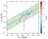 |
Fig. 2. νc, z − Liso relation obtained from the synchrotron single-bin sample. The color scale is associated with the frequency ratio, νm/νc, derived from the synchrotron fit. The straight black line represents the best-fit line from the linear fit, and the green-shaded area the relative 3σ scatter region. |
3.3. Multiple-bins analysis
Of the 74 GRBs in our total sample, we selected the 15 GRBs with the highest fluence (reported by Fermi/GBM catalog) in order to perform time-resolved spectral analyses across their whole duration. Among these 15 GRBs, we found GRB090902B and GRB190114C; namely, the two GRBs exhibiting a second power law spectral component in addition to the main one. We removed these two GRBs from the sample, and the remaining 13 GRBs constitute the new multiple-bin sample. The time-resolved spectral analysis relative to this sample includes both Band and synchrotron models, similar to the procedure described in Sect. 2. We visually selected the time bins from the background-subtracted light curve of the best NaI detector in GBM. The time-bin start and stop were chosen in order to match as closely as possible pulses or single emission episodes shown in the GRB light curve. The time-bin width was chosen in order to collect enough signal for the spectral analysis. In case of particularly bright pulses, they were divided into multiple time bins given the high signal. In this sample, every time bin has a signal-to-noise ratio of SNR > 30. We included LLE spectral data in any time bin where they were available.
The multiple-bin sample covers a total of 125 spectra. The GRB list, their time bins, and the spectral fit results are reported in Table B.1. According to the Bayes factor, 65 spectra are best fit by synchrotron model, 48 spectra are best fit by Band, and for 12 spectra the Bayes factor cannot determine which is the best-fit model. For the 48 spectra best fit by Band, we report the Ep,z, Liso, and α estimates obtained from the Band model, whereas for the remaining 77 spectra we report Ep,z, Liso, and νc, z obtained from the synchrotron model.
Similarly to the analysis of the single-bin sample, we observe that the fit with the synchrotron model does not return any Ep,z−Liso relation. However, restricting the multi-bin sample to its synchrotron subsample (i.e., the 77 GRBs for which we report synchrotron results), we observe again a very tight correlation between νc, z and Liso (Fig. 3). The Spearman’s rank correlation coefficient is ρ = 0.83 with chance probability of Pchance = 1.83 × 10⁻²⁰ (Table 2).
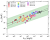 |
Fig. 3. νc, z − Liso relation obtained from the synchrotron GRBs in the multi-bin sample. We show multiple time bins from different GRBs with circles of the same colors. The number inside the circles represents the bin number that data point is associated with. The straight black line represents the best-fit line from the linear fit, while the dashed-line the best-fit line obtained from the νc, z − Liso relation in the single-bin sample. The green-shaded area shows the 3σ scatter region of the relation. |
We notice that the νc, z − Liso relation derived in this way is described by a slightly flatter best-fit line, with a slope of m = 0.41 ± 0.03 and normalization of K = 1.12 ± 0.09, whereas the intrinsic scatter is comparable (σsc = 0.31). It is worth mentioning that, if the GRB211211A time-resolved dataset is considered alone, it is consistent with a slope of m ∼ 0.5. If excluded from the multiple-bin sample, the relative νc, z − Liso relation has the same slope as the one obtained from the single-bin one.
4. Discussion
We found a novel νc, z − Liso relation by employing a physical synchrotron model to describe the prompt emission of GRBs observed by Fermi/GBM. The fact that this new relation is found with high significance in the single-bin and multiple-bin samples, where both the emissions during the peak and across the whole burst duration are explored, strongly points toward its possible physical nature. In the following, we provide an interpretation of these results.
In the internal shocks framework, synchrotron spectra have a peak energy, Ep,z, which depends on many other parameters, most relevantly the bulk Lorentz factor, Γ, and the dynamical timescale, tvar (Rees & Mészáros 2005). The presence of a Ep,z−Liso correlation would imply that Γ and tvar are the same for all the GRBs. This condition is not supported by any observation in large GRB samples. Therefore, this scenario is not in accordance with the Yonetoku relation, and our findings point toward this conclusion.
As a matter of fact, when time-resolved spectral analysis is performed, Ep,z exhibits a strong spectral evolution, which can track the intensity of the pulse (e.g., Golenetskii et al. 1983) or show a hard-to-soft transition (e.g., Lu et al. 2012). The latter case is not consistent with the Yonetoku relation when multiple pulses are present. On the other hand, Ravasio et al. (2019) performed time resolved analysis of a sample of ten bright long GRBs, fitting their spectra with a double smoothly broken power law (2SBPL) function, namely a Band function with two power laws before the peak. They find that the break energy, consistent with the synchrotron break in a marginally fast-cooling regime, does not vary much across the GRB duration. This finding suggests that the break energy may be more “standard” than the peak energy, or at least have minor dependencies on other parameters. However, the values of peak and break energies obtained through 2SBPL fits do not necessarily coincide with synchrotron breaks due to the shape of synchrotron spectra.
The question arises of whether and how the νc, z − Liso relation can agree with almost two decades of observations pointing toward correlations with the peak energy, Ep,z. A synchrotron SED in fast-cooling regime (νm/νc > 1) exhibits two typical energies: a peak around νm and a break around νc. Before the peak, we expect a hard photon index of α1 = −2/3 for E < hνc, while for hνc < E < hνm the emission softens with a photon index of α2 = −3/2. The smaller the frequency ratio, νm/νc, is, the closer the two breaks are.
Historically, most of the spectral fits that lead to the Yonetoku relation were carried out using phenomenological models, which allowed for only one power law segment at low energies, with a single spectral break coinciding with the peak. In the hypothesis that GRBs prompt spectra are produced by synchrotron processes, the fit of a single-break model (such as the Band function) to a spectrum that intrinsically presents two breaks (such as a synchrotron one) can lead to two main observational biases:
-
(1.)
It appears that, when a single-break model like Band is fit to an intrinsic double-break model, it returns
 , where
  is the Band peak energy, whereas Eb and Ep are break and peak energies. Therefore, the fit of a two-breaks model to a suitable spectrum leads to systematically larger Ep,z.
 -
(2.)
The low-energy spectral index, α, which one obtains fitting a single-break model, is a weighted average of the two spectral indices, α1 and α2, before and after the break, respectively (Toffano et al. 2021). Therefore, the hardness of the spectrum depends on the proximity of Eb to Ep.
By comparing results from the Band and synchrotron models related to the single-bin synchrotron sample, we observe a similar pattern. In fact, when the synchrotron fit returns a fast-cooling spectrum, its peak energy,  , is systematically larger than the value obtained by fitting the Band model,
  . Conversely, when 1< νm/νc < 3, the two frequencies are very close and break and peak energies are hardly distinguishable. The Band and synchrotron fits return similar peak energies; that is,
  (Fig. 4, left panel).
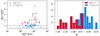 |
Fig. 4. Ratio between the rest-frame peak energy from synchrotron model fits, |


In Fig. 4 (right panel), we show the distributions of the photon index, α, associated with the fast-cooling and intermediate-cooling spectra. While fast-cooling spectra span a large range of values pointing to softer spectra, the intermediate-cooling spectra exhibit harder photon indices close to α = −0.67, which is the value expected for E < Eb, z = hνc, z.
We can conclude that the effect of fitting a single-break model such as the Band function to a synchrotron spectrum leads to systematically lower values of Ep,z. These are the premises by which the Yonetoku relation was vastly studied in the literature. According to these findings, it is not surprising that when a physical synchrotron model is used in testing the Yonetoku relation, the latter holds only for GRBs where 1< νm/νc < 3, namely when peak and break energies nearly coincide, and therefore Band fits return correct Ep,z estimates. This suggests that, at least for the GRBs that can be correctly described by an idealized synchrotron model, the underlying physical relation that holds is the νc, z − Liso one. When spectra are analyzed with the Band function,  is not far from hνc, z, returning the notorious Yonetoku relation. However, when a second break is accounted for, the Yonetoku relation does not hold anymore, and the new νc, z − Liso appears to be the underlying relation.
In Fig. 5, we show an example of this phenomenon for GRB160625B, one of the brightest sources in the multiple-bin sample. Its time-resolved analysis shows that, during the time bins in which the spectrum is in the fast-cooling regime, the corresponding Ep,z and Liso are outliers of the Yonetoku relation. As soon as its spectrum shows an intermediate-cooling state, its Ep,z approaches the relative νc, z and the corresponding Ep,z and Liso follow the Yonetoku relation.
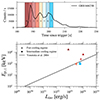 |
Fig. 5. Fermi/GBM (8–900 keV) light curve and time bins of the associated time-resolved analysis of GRB160625B (upper panel). In the lower panel, we show the relative Ep,z−Liso plane. The color scale is associated with the time bin in which the spectral analysis was performed. We show, for this GRB, the results of the synchrotron fit, and we represent the bins with fast-cooling spectra as triangles, and the bins with intermediate-cooling spectra as squares. The straight black line represents the Yonetonu relation obtained from Yonetoku et al. (2004). |
Nonetheless, Guiriec et al. (2013, 2015a) discuss an opposite scenario. They fit a two-components model to time-resolved GRB prompt spectra. The presence of a second peaked component at lower energies resembles (in the photon flux representation) a total spectrum with two breaks. Despite finding systematically larger Ep,z with respect to single-break model fits, they claim a tighter Yonetoku relation when a second component is accounted for in the fit. This behavior was proven in a sample of five GRBs (e.g., Guiriec et al. 2015b). However, the extension of this to larger samples would contrast with the findings of Ep,z−Liso relations in numerous samples when single-break models are used. In fact, if both the Ep,z increase and the Yonetoku relation from single-break models constitute valid observational evidence, the fit of a second thermal component (or a double-break model) would systematically bring GRBs out of the relation. In this scenario, the only way to have a tighter relation would be for these GRBs exhibiting breaks to be all systematically beneath the best-fit line; in other words, to be scattered away from the best-fit relation with systematically lower Ep,z for the same Liso. Nonetheless, this hypothesis is hard to test in a small sample. In this work, testing a large sample of GRBs, we instead observed that GRBs in synchrotron subsamples do not preferentially lie underneath the best-fit line, and this leads to the absence of the Yonetoku relation in both our samples.
It is important to stress that the results derived from the single-bin sample are obtained under the assumption of synchrotron being the main radiative process producing prompt emission. This hypothesis is verified through model comparison only for 21/74 GRBs. On the other hand, as is also discussed in Toffano et al. (2021), the comparison between physical and phenomenological models is quite tricky, the peculiar synchrotron features being lost in low signal-to-noise spectra, often favoring a Band function. However, the conclusions that we draw in this analysis are valid as long as the synchrotron model provides a good fit to the data, hence returning reliable estimates of both νm and νc. Nevertheless, the results drawn from the multiple-bin sample go beyond this assumption, selecting only synchrotron spectra through model comparison.
In this regard, one important result of this work is the fact that the synchrotron model we used to fit the data is not able to describe all the spectra well. The interpretation can be twofold: it appears that prompt dissipation sites and/or radiative processes are not the same for all the GRBs (therefore synchrotron emission cannot explain all GRB spectra), or that the synchrotron model we use is too simplistic to account for the GRB spectra.
From the single-bin Band subsample (Table A.2), we notice that the spectra that reject the synchrotron model show a relatively hard spectral index, α. The presence of these hard prompt emission spectra are in tension with a synchrotron interpretation, pointing to other emission mechanisms possibly produced in the optically thick region. However, we performed an additional fit of GRB spectra in the single-bin Band subsample, restricting the dataset between 8–30 keV and fitting a power law model. We excluded from this analysis GRB190114C and GRB090902B, since their low-energy spectrum at a few keV is dominated by a second power law component.
We observe that the spectral indices obtained through the power law fit, αPL, is much smaller (therefore the spectra are softer) than the ones obtained through Band fits, αBand (Fig. 6). In particular, the αPL values obtained are close to the value of α = −0.67, expected from synchrotron spectra at energies of E < Eb. The reason for this mismatch could be the fact that the photon index, α, of the Band function is degenerate with the smoothness and position of the spectral peak. This finding suggests that α may be a biased indicator of GRB hardness (Burgess et al. 2015).
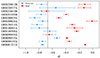 |
Fig. 6. Low-energy spectral index, α, obtained by fitting a Band model (in red) or a power law model considering data between 8–30 keV (in blue). The fit was performed to GRBs in the single-bin Band subsample. The dashed vertical line corresponds to α = −0.67, the value expected in synchrotron spectra for E < Eb. Errors are reported with a 68% confidence level. |
Still, the synchrotron model used in this work is not able to provide a good representation of the data for 13 GRBs. We propose that this fact is due not to the violation of the single electron spectrum, as is often stated in the literature, but rather the shape and smoothness of the spectral profile around the peak. In these regards, there are many processes not accounted for in our modeling, such as inverse Compton scattering in the Klein-Nishina regime (Derishev 2009; Bošnjak et al. 2009; Daigne et al. 2011) provided by decaying magnetic fields (Pe’er & Zhang 2006; Derishev 2007; Zhao et al. 2014; Daigne & Bošnjak 2024), anisotropic pitch angle distribution (Medvedev 2000; Sobacchi et al. 2021), and so on. Accounting for all these processes may lead to spectra more in accordance with the observations, without the need to introduce different radiative processes.
When instead a simple synchrotron model also describes the data well, we see a particular trend. All the GRBs in the synchrotron subsample are in (marginally) fast-cooling regime, as was expected from other works (Ravasio et al. 2019).
Interestingly, the majority of them are in the intermediate-cooling regime, which is a specific stage of a marginally fast-cooling regime in which the two main frequencies, νm and νc, are coincident. Nearly 60% of GRBs in the single-bin synchrotron sample are in this state, at odds with the ∼25% of GRBs in the multiple-bins synchrotron sample. This suggests that this state is reached more frequently in the brightest pulses.
5. Conclusions
In this work, we have performed spectral analysis of GRBs in two samples: the single-bin sample (with 74 GRBs, one spectrum with 1s exposure per GRB during their peak) and the multiple-bin sample (with 13 bright GRBs, multiple spectra with exposures of a few seconds per GRB for a total of 125 spectra).
In both these samples, we fit two main models. The first one is the Band function, which phenomenologically describes GRB spectra without any assumption about the underlying physics. In addition, we used a simple physical model that accounts for power law-distributed relativistic electrons cooling down through synchrotron radiation.
We aim to test the validity of the Ep,z−Liso (Yonetoku) relation using both Band and synchrotron models. While the former was the one historically used to derive GRB empirical relations, the introduction of a synchrotron model, which is a viable explanation for GRB prompt spectra, allows us to better investigate the nature of this emission and the relative empirical relations. We summarize the main results of this work in the following:
-
We show that most of the GRBs in the single-bin sample are well fit by the synchrotron model (58/74). However, there are GRBs whose spectrum cannot be described by a synchrotron model, preferring instead a Band function (16/74). Nonetheless, GRBs that prefer a Band model, when fit with a power law at E < 30 keV, exhibit a photon index of αPL ≲ −0.7; in other words, they do not violate the single electron spectrum.
-
It appears that all the GRBs for which we report results from the synchrotron fit are in a fast-cooling regime (νm/νc > 1). The majority of these ones show particular νm/νc values, where νm (i.e., the spectral peak) is only slightly larger than νc (i.e., the synchrotron break). We refer to these cases as GRBs in an intermediate-cooling state, a particular case of marginally fast-cooling spectra where the break and the peak energies are basically coincident (1< νm/νc < 3).
-
We show that the fit of the Band model (single-break spectrum) to a possibly intrinsic synchrotron spectrum (double-break spectrum) leads to systematically lower Ep,z and the proximity of Eb, z to Ep,z influences the hardness of the spectrum; namely, the low-energy spectral index, α, fit with the Band model.
-
We observe that GRBs in the single-bin sample do not follow the Yonetoku relation unless they are in an intermediate-cooling state; that is, the peak and break energies are extremely close to each other.
-
We find a novel tight relation between the rest-frame cooling frequency, νc, z, and the isotropic-equivalent luminosity:
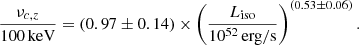
This relation is found in both single-bin and multiple-bin samples, with slightly different slopes.
The underlying assumption of this work is that prompt emission spectra are produced through synchrotron cooling of power-law distributed particles. Nonetheless, in the multiple-bin sample analysis we report synchrotron fit results whenever the model comparison does not discard the synchrotron model. This points toward the physical nature of the νc, z − Liso relation.
We show that, if GRB prompt emission is produced through synchrotron radiation, the fit using a Band function does not always represent a good spectral description. For example, a Band fit would return a peak energy estimate,  , in between hνc, z and
  . This suggests that, for synchrotron spectra, the fundamental physical relation is between Liso and νc, z. The Yonetoku relation, which was found through Band fits, can be the effect of a single-break model fit to a double-break spectrum. Given the occurrence of GRB spectra in intermediate-cooling regimes (or in general in marginally fast-cooling regimes),
  provides a proxy of νc, z. The higher the intrinsic ratio, νm/νc, the higher the scatter of that GRB relative to the Yonetoku relation.
This novel interpretation of the Yonetoku relation constitutes a step forward in understanding the physics behind empirical relations and prompt emission. For the prompt synchrotron spectra, we found a new tight relation that connects the cooling regime with the total luminosity of the burst: the less it cools, the brighter it is.
This behavior is counterintuitive. One would expect, in the optically thin synchrotron framework, more radiative output when particles cool down, interacting with stronger magnetic fields. This new relation can constitute a benchmark in testing GRB prompt emission models, and push forward the possibility of using GRBs to constrain cosmological properties. The recent launch of the SVOM and Einstein Probe missions can provide, in synergies with past observatories, a variety of GRB observations with measured redshift and extend the empirical correlations study with a particularly soft burst emitting in the X-rays.
Data availability
Fermi/GBM raw data are publicly available in the Fermi GBM Burst Catalog: https://heasarc.gsfc.nasa.gov/W3Browse/fermi/fermigbrst.html. Fermi/LAT Low Energy (LLE) data are publicly available in the Fermi LAT Low-Energy Events Catalog: https://heasarc.gsfc.nasa.gov/W3Browse/fermi/fermille.html. The result of the single-bin and multiple-bin samples, together with the spectral fit plots, are available at the following link: https://zenodo.org/records/14205680
Acknowledgments
The authors thank B. Banerjee, D. Bjørn Malesani, M. Branchesi, A. Celotti, G. Ghirlanda, G. Ghisellini, L. Nava and O.S. Salafia for the fruitful discussions about this work. AM thanks the Cosmic Dawn Center in Copenhagen and the Observatory of Brera in Merate for the hospitality during the development of this project.
References
- Abbott, B. P., Abbott, R., Abbott, T. D., et al. 2017, ApJ, 848, L13 [CrossRef] [Google Scholar]
- Abdo, A. A., Ackermann, M., Ajello, M., et al. 2009, ApJ, 706, L138 [NASA ADS] [CrossRef] [Google Scholar]
- Ajello, M., Arimoto, M., Axelsson, M., et al. 2020, ApJ, 890, 9 [Google Scholar]
- Amati, L., Frontera, F., Tavani, M., et al. 2002, A&A, 390, 81 [NASA ADS] [CrossRef] [EDP Sciences] [Google Scholar]
- Arnaud, K. A. 1996, ASP Conf. Ser., 101, 17 [Google Scholar]
- Band, D. L., & Preece, R. D. 2005, ApJ, 627, 319 [Google Scholar]
- Band, D., Matteson, J., Ford, L., et al. 1993, ApJ, 413, 281 [Google Scholar]
- Berger, E. 2014, ARA&A, 52, 43 [CrossRef] [Google Scholar]
- Bhat, P. N., Briggs, M. S., Connaughton, V., et al. 2012, ApJ, 744, 141 [NASA ADS] [CrossRef] [Google Scholar]
- Bošnjak, Ž., Daigne, F., & Dubus, G. 2009, A&A, 498, 677 [NASA ADS] [CrossRef] [EDP Sciences] [Google Scholar]
- Buchner, J. 2016, Astrophysics Source Code Library [record ascl:1610.011] [Google Scholar]
- Burgess, J. M., Ryde, F., & Yu, H.-F. 2015, MNRAS, 451, 1511 [Google Scholar]
- Burgess, J. M., Bégué, D., Greiner, J., et al. 2020, Nat. Astron., 4, 174 [Google Scholar]
- Butler, N. R., Kocevski, D., Bloom, J. S., & Curtis, J. L. 2007, ApJ, 671, 656 [Google Scholar]
- D’Agostini, G. 2005, arXiv e-prints [arXiv:physics/0511182] [Google Scholar]
- Daigne, F., & Bošnjak, 2024, A&A in press, https://doi.org/10.1051/0004-6361/202451369 [Google Scholar]
- Daigne, F., Bošnjak, Ž., & Dubus, G. 2011, A&A, 526, A110 [NASA ADS] [CrossRef] [EDP Sciences] [Google Scholar]
- Derishev, E. V. 2007, Ap&SS, 309, 157 [NASA ADS] [CrossRef] [Google Scholar]
- Derishev, E. V. 2009, IJMPD, 18, 1523 [NASA ADS] [CrossRef] [Google Scholar]
- Drenkhahn, G., & Spruit, H. C. 2002, A&A, 391, 1141 [NASA ADS] [CrossRef] [EDP Sciences] [Google Scholar]
- Eichler, D., Livio, M., Piran, T., & Schramm, D. N. 1989, Nature, 340, 126 [NASA ADS] [CrossRef] [Google Scholar]
- Foreman-Mackey, D., Hogg, D. W., Lang, D., & Goodman, J. 2013, PASP, 125, 306 [Google Scholar]
- Ghirlanda, G., Nava, L., Ghisellini, G., Firmani, C., & Cabrera, J. I. 2008, MNRAS, 387, 319 [Google Scholar]
- Ghirlanda, G., Nava, L., Ghisellini, G., Celotti, A., & Firmani, C. 2009, A&A, 496, 585 [NASA ADS] [CrossRef] [EDP Sciences] [Google Scholar]
- Ghirlanda, G., Nava, L., & Ghisellini, G. 2010, A&A, 511, A43 [NASA ADS] [CrossRef] [EDP Sciences] [Google Scholar]
- Ghirlanda, G., Ghisellini, G., & Nava, L. 2011a, MNRAS, 418, L109 [Google Scholar]
- Ghirlanda, G., Ghisellini, G., Nava, L., & Burlon, D. 2011b, MNRAS, 410, L47 [NASA ADS] [CrossRef] [Google Scholar]
- Ghisellini, G., & Celotti, A. 1999, ApJ, 511, L93 [Google Scholar]
- Golenetskii, S. V., Mazets, E. P., Aptekar, R. L., & Ilinskii, V. N. 1983, Nature, 306, 451 [NASA ADS] [CrossRef] [Google Scholar]
- Gompertz, B. P., Ravasio, M. E., Nicholl, M., et al. 2023, Nat. Astron., 7, 67 [Google Scholar]
- Gruber, D., Goldstein, A., Weller von Ahlefeld, V., et al. 2014, ApJS, 211, 12 [Google Scholar]
- Guiriec, S., Daigne, F., Hascoët, R., et al. 2013, ApJ, 770, 32 [NASA ADS] [CrossRef] [Google Scholar]
- Guiriec, S., Kouveliotou, C., Daigne, F., et al. 2015a, ApJ, 807, 148 [NASA ADS] [CrossRef] [Google Scholar]
- Guiriec, S., Mochkovitch, R., Piran, T., et al. 2015b, ApJ, 814, 10 [NASA ADS] [CrossRef] [Google Scholar]
- Kaneko, Y., Preece, R. D., Briggs, M. S., et al. 2006, ApJS, 166, 298 [CrossRef] [Google Scholar]
- Kass, R. E., & Raftery, A. E. 1995, J. Am. Stat. Assoc., 90, 773 [Google Scholar]
- Lazzati, D., Ghisellini, G., Celotti, A., & Rees, M. J. 2000, ApJ, 529, L17 [NASA ADS] [CrossRef] [Google Scholar]
- Lloyd, N. M., & Petrosian, V. 2000, ApJ, 543, 722 [NASA ADS] [CrossRef] [Google Scholar]
- Lloyd-Ronning, N. M., & Petrosian, V. 2002, ApJ, 565, 182 [NASA ADS] [CrossRef] [Google Scholar]
- Lu, R.-J., Wei, J.-J., Liang, E.-W., et al. 2012, ApJ, 756, 112 [Google Scholar]
- Medvedev, M. V. 2000, ApJ, 540, 704 [NASA ADS] [CrossRef] [Google Scholar]
- Meegan, C., Lichti, G., Bhat, P. N., et al. 2009, ApJ, 702, 791 [Google Scholar]
- Mészáros, P., & Rees, M. J. 2000, ApJ, 530, 292 [Google Scholar]
- Minaev, P. Y., & Pozanenko, A. S. 2020, MNRAS, 492, 1919 [NASA ADS] [CrossRef] [Google Scholar]
- Nakar, E., & Piran, T. 2005, MNRAS, 360, L73 [Google Scholar]
- Narayan, R., Paczynski, B., & Piran, T. 1992, ApJ, 395, L83 [NASA ADS] [CrossRef] [Google Scholar]
- Nava, L., Ghirlanda, G., Ghisellini, G., & Firmani, C. 2008, MNRAS, 391, 639 [Google Scholar]
- Nava, L., Salvaterra, R., Ghirlanda, G., et al. 2012, MNRAS, 421, 1256 [Google Scholar]
- Oganesyan, G., Nava, L., Ghirlanda, G., & Celotti, A. 2017, ApJ, 846, 137 [Google Scholar]
- Oganesyan, G., Nava, L., Ghirlanda, G., & Celotti, A. 2018, A&A, 616, A138 [NASA ADS] [CrossRef] [EDP Sciences] [Google Scholar]
- Oganesyan, G., Nava, L., Ghirlanda, G., Melandri, A., & Celotti, A. 2019, A&A, 628, A59 [NASA ADS] [CrossRef] [EDP Sciences] [Google Scholar]
- Paczynski, B. 1986, ApJ, 308, L43 [NASA ADS] [CrossRef] [Google Scholar]
- Parsotan, T., & Ito, H. 2022, Universe, 8, 310 [NASA ADS] [CrossRef] [Google Scholar]
- Pe’er, A. 2008, ApJ, 682, 463 [NASA ADS] [CrossRef] [Google Scholar]
- Pe’er, A., & Zhang, B. 2006, ApJ, 653, 454 [NASA ADS] [CrossRef] [Google Scholar]
- Preece, R. D., Briggs, M. S., Mallozzi, R. S., et al. 1998, ApJ, 506, L23 [Google Scholar]
- Ravasio, M. E., Ghirlanda, G., Nava, L., & Ghisellini, G. 2019, A&A, 625, A60 [NASA ADS] [CrossRef] [EDP Sciences] [Google Scholar]
- Rees, M. J., & Meszaros, P. 1994, ApJ, 430, L93 [Google Scholar]
- Rees, M. J., & Mészáros, P. 2005, ApJ, 628, 847 [NASA ADS] [CrossRef] [Google Scholar]
- Salafia, O. S., & Ghirlanda, G. 2022, Galaxies, 10, 93 [NASA ADS] [CrossRef] [Google Scholar]
- Sari, R., & Piran, T. 1997, ApJ, 485, 270 [NASA ADS] [CrossRef] [Google Scholar]
- Shahmoradi, A., & Nemiroff, R. J. 2011, MNRAS, 411, 1843 [Google Scholar]
- Sobacchi, E., Sironi, L., & Beloborodov, A. M. 2021, MNRAS, 506, 38 [NASA ADS] [CrossRef] [Google Scholar]
- Toffano, M., Ghirlanda, G., Nava, L., et al. 2021, A&A, 652, A123 [NASA ADS] [CrossRef] [EDP Sciences] [Google Scholar]
- Tsvetkova, A., Frederiks, D., Golenetskii, S., et al. 2017, ApJ, 850, 161 [NASA ADS] [CrossRef] [Google Scholar]
- Ursi, A., Tavani, M., Frederiks, D. D., et al. 2020, ApJ, 904, 133 [NASA ADS] [CrossRef] [Google Scholar]
- von Kienlin, A., Meegan, C. A., Paciesas, W. S., et al. 2020, ApJ, 893, 46 [Google Scholar]
- Wang, W.-K., Xie, W., Gao, Z.-F., et al. 2024, Res. Astron. Astrophys., 24, 025006 [CrossRef] [Google Scholar]
- Woosley, S. E. 1993, ApJ, 405, 273 [Google Scholar]
- Woosley, S. E., & Bloom, J. S. 2006, ARA&A, 44, 507 [Google Scholar]
- Yonetoku, D., Murakami, T., Nakamura, T., et al. 2004, ApJ, 609, 935 [Google Scholar]
- Yonetoku, D., Murakami, T., Tsutsui, R., et al. 2010, PASJ, 62, 1495 [NASA ADS] [Google Scholar]
- Zhang, B., & Yan, H. 2011, ApJ, 726, 90 [Google Scholar]
- Zhang, B., Zhang, B.-B., Virgili, F. J., et al. 2009, ApJ, 703, 1696 [NASA ADS] [CrossRef] [Google Scholar]
- Zhao, X., Li, Z., Liu, X., et al. 2014, ApJ, 780, 12 [Google Scholar]
Appendix A: Single-bin sample tables
Bursts in the single-bin sample, synchrotron subsample.
Bursts in the single-bin sample, Band subsample.
Appendix B: Multiple-bin sample tables
Bursts in the multiple-bin sample.
All Tables
Results of the statistical analysis on the Ep, z − Liso and νc, z − Liso relations.
All Figures
|
Fig. 1. Yonetoku relation obtained from the single-bin sample. Black stars represent GRBs from the Band subsample, while colored dots represent GRBs from the synchrotron subsample. The color scale is associated with the frequency ratio, νm/νc, derived from the synchrotron fit. We fit a power law to the whole single-bin sample (left-hand panel) and to the GRBs in the synchrotron subsample in an intermediate cooling regime (right-hand panel). The straight black line represents the best-fit line from the linear fit, and the green-shaded area the relative 3σ scatter region. For comparison, the dashed black line represents the best-fit line from Yonetoku et al. (2004). |
| In the text | |
|
Fig. 2. νc, z − Liso relation obtained from the synchrotron single-bin sample. The color scale is associated with the frequency ratio, νm/νc, derived from the synchrotron fit. The straight black line represents the best-fit line from the linear fit, and the green-shaded area the relative 3σ scatter region. |
| In the text | |
|
Fig. 3. νc, z − Liso relation obtained from the synchrotron GRBs in the multi-bin sample. We show multiple time bins from different GRBs with circles of the same colors. The number inside the circles represents the bin number that data point is associated with. The straight black line represents the best-fit line from the linear fit, while the dashed-line the best-fit line obtained from the νc, z − Liso relation in the single-bin sample. The green-shaded area shows the 3σ scatter region of the relation. |
| In the text | |
|
Fig. 4. Ratio between the rest-frame peak energy from synchrotron model fits, |
| In the text | |
|
Fig. 5. Fermi/GBM (8–900 keV) light curve and time bins of the associated time-resolved analysis of GRB160625B (upper panel). In the lower panel, we show the relative Ep,z−Liso plane. The color scale is associated with the time bin in which the spectral analysis was performed. We show, for this GRB, the results of the synchrotron fit, and we represent the bins with fast-cooling spectra as triangles, and the bins with intermediate-cooling spectra as squares. The straight black line represents the Yonetonu relation obtained from Yonetoku et al. (2004). |
| In the text | |
|
Fig. 6. Low-energy spectral index, α, obtained by fitting a Band model (in red) or a power law model considering data between 8–30 keV (in blue). The fit was performed to GRBs in the single-bin Band subsample. The dashed vertical line corresponds to α = −0.67, the value expected in synchrotron spectra for E < Eb. Errors are reported with a 68% confidence level. |
| In the text | |
Current usage metrics show cumulative count of Article Views (full-text article views including HTML views, PDF and ePub downloads, according to the available data) and Abstracts Views on Vision4Press platform.
Data correspond to usage on the plateform after 2015. The current usage metrics is available 48-96 hours after online publication and is updated daily on week days.
Initial download of the metrics may take a while.