| Issue |
A&A
Volume 694, February 2025
|
|
|---|---|---|
| Article Number | A323 | |
| Number of page(s) | 19 | |
| Section | Extragalactic astronomy | |
| DOI | https://doi.org/10.1051/0004-6361/202452268 | |
| Published online | 24 February 2025 | |
Extragalactic magnetar giant flare GRB 231115A: Insights from Fermi/GBM observations
1
Department of Physics & Astronomy, Louisiana State University, Baton Rouge, LA 70803, USA
2
Department of Physics, The George Washington University, 725 21st Street NW, Washington, DC 20052, USA
3
Department of Physics and Astronomy - MS 108, Rice University, 6100 Main Street, Houston, TX 77251-1892, USA
4
Ioffe Institute, 26 Politekhnicheskaya, St. Petersburg 194021, Russia
5
SRON Netherlands Institute for Space Research, Niels Bohrweg 4, NL-2333 CA Leiden, the Netherlands
6
McWilliams Center for Cosmology and Astrophysics, Department of Physics, Carnegie Mellon University, 5000 Forbes Avenue, Pittsburgh, PA 15213, USA
7
Science and Technology Institute, Universities Space and Research Association, 320 Sparkman Dr., Huntsville, AL 35805, USA
8
Astrophysics Science Division, NASA/GSFC, Greenbelt, MD 20771, USA
9
Department of Astronomy, University of Maryland, College Park, MD 20742, USA
10
Center for Research and Exploration in Space Science and Technology, NASA/GSFC, Greenbelt, MD 20771, USA
11
CRESST, Center for Space Sciences and Technology, UMBC, Baltimore, MD 210250, USA
12
Department of Space Science, University of Alabama in Huntsville, Huntsville, AL 35899, USA
13
Center for Space Plasma and Aeronomic Research, University of Alabama in Huntsville, Huntsville, AL 35899, USA
14
University Observatory, Faculty of Physics, Ludwig-Maximilians-Universität München, Scheinerstr. 1, 81679 Munich, Germany
15
Excellence Cluster ORIGINS, Boltzmannstr. 2, 85748 Garching, Germany
16
Department of Physics, George Washington University, Corcoran Hall, 725 21st Street NW, Washington, DC 20052, USA
17
Max Planck Institute for Extraterrestrial Physics, Giessenbachstrasse, D-85748 Garching, Germany
⋆ Corresponding author; This email address is being protected from spambots. You need JavaScript enabled to view it.
Received:
16
September
2024
Accepted:
27
January
2025
Abstract
Magnetar giant flares (MGFs) are the extremely short, energetic transients originating from highly magnetized neutron stars. When observed in nearby galaxies, these rare events are nearly indistinguishable from cosmological short gamma-ray bursts. We present the analysis of GRB 231115A, a candidate extragalactic MGF observed by Fermi/GBM and localized by INTEGRAL to the starburst galaxy M82. This burst exhibits distinctive temporal and spectral characteristics, including a short duration and a high peak energy, consistent with known MGFs. Time-resolved analysis reveals rapid spectral evolution and a clear correlation between luminosity and spectral hardness, providing robust evidence of relativistic outflows. Archival Chandra data identified point sources within the GRB 231115A localization consistent with the theoretical maximum persistent emission luminosity, though no definitive counterpart was found. Simulations indicate that any transient emission associated with GRB 231115A would require energies exceeding those of typical magnetar bursts to be detectable by current instruments. While the tail of a MGF originating from outside of the Milky Way and its satellite galaxies has never been detected, analysis suggests that such emission could be observable at M82’s distance with instruments like Swift/XRT or NICER, though no tail was identified for this event. These findings underscore the need for improved follow-up strategies and technological advancements to enhance MGF detection and characterization.
Key words: stars: magnetars / stars: neutron
© The Authors 2025
 Open Access article, published by EDP Sciences, under the terms of the Creative Commons Attribution License (https://creativecommons.org/licenses/by/4.0), which permits unrestricted use, distribution, and reproduction in any medium, provided the original work is properly cited.
This article is published in open access under the Subscribe to Open model. This email address is being protected from spambots. You need JavaScript enabled to view it. to support open access publication.
1. Introduction
Gamma-ray bursts (GRBs) are transient phenomena characterized by the emission of high-energy electromagnetic radiation in the 10 keV to 100 GeV bands. These bursts can persist for durations ranging from a few milliseconds to several minutes (Kouveliotou et al. 2012). GRBs can potentially exhibit apparent luminosities that surpass those of typical supernovae by factors of hundreds and temporarily become the most luminous source of gamma-ray photons in the cosmos. GRBs are traditionally classified into two categories: short GRBs, which last less than two seconds, and long GRBs, which last more than two seconds. These two GRB populations differ not only in duration but also in their spectral properties (Kouveliotou et al. 1993; von Kienlin et al. 2020).
Long GRBs make up the majority of current gamma-ray detections and are conventionally attributed to collapsars (Woosley & Bloom 2006). Short GRBs are attributed to two possible progenitors. The first, which makes up the vast majority of short GRBs, is the merger of compact objects, such as two neutron stars or a neutron star and a black hole (Eichler et al. 1989; Fong et al. 2015). These mergers may also produce a reasonable fraction of long GRBs (Rastinejad et al. 2022; Troja et al. 2022; Veres et al. 2023). The compact object merger theory was substantiated by the detection of a gravitational wave event on 17 August 2017, which coincided with a short GRB resulting from the coalescence of two neutron stars (Abbott et al. 2017a,b; Goldstein et al. 2017).
The second source of short GRBs is the bright explosions from highly magnetized neutron stars (i.e., magnetars; Duncan & Thompson 1992; Thompson & Duncan 1995) in nearby galaxies. Galactic magnetars have been observed emitting short, hard X-ray bursts and, on rare occasions, extremely energetic events known as magnetar giant flares (MGFs; Kaspi & Beloborodov 2017). MGFs are characterized by a brief, milliseconds-long spike in gamma-ray emission. This initial spike is far more energetic than those observed in typical magnetar burst spectra, with high isotropic-equivalent energies (Eiso ∼ 1044 − 1046 erg). The bright, hard spike is followed by a much softer, weaker tail, which can last several minutes, modulated in flux and spectral hardness by the spin period of the neutron star from which it originates (Hurley et al. 1999; Palmer et al. 2005). Only three such events have been detected and confirmed to date: two from Galactic sources, SGR 1900+14 (Hurley et al. 1999; Feroci et al. 1999) and SGR 1806-20 (Palmer et al. 2005; Frederiks et al. 2007a), and one from magnetar SGR 0526-66 in the Large Magellanic Cloud (Mazets et al. 1979; Fenimore et al. 1996). The initial peak of all three events was so bright that they saturated nearly all directly observing detectors.
At extragalactic distances beyond 3 Mpc, the rotationally modulated tail indicative of a MGF is too faint to be detected with current instruments due to their sensitivity limitations. Consequently, the absence of this tail would cause MGFs from nearby galaxies to resemble, and thus be misidentified as, cosmological short GRBs (Mazets et al. 1982; Eichler et al. 1989; Duncan 2001; Hurley et al. 2005; Palmer et al. 2005; Hurley 2011), presenting a challenge in identifying MGFs that originate outside the Milky Way. This misidentification may account for a portion of short GRB events, with one statistical estimate putting the number at ∼2% (Burns et al. 2021). Therefore, localizing short GRBs that resemble MGFs to nearby star-forming galaxies is the most reliable method for differentiating MGFs from cosmological short GRBs.
Currently, there are five short GRBs that, based on convincing evidence of their temporal and spectral characteristics, and with localizations by the Interplanetary Network (IPN; Klebesadel et al. 1973) coinciding with nearby star-forming galaxies, have been identified as extragalactic MGF candidates. The first, GRB 051103 (Ofek et al. 2006; Frederiks et al. 2007b; Hurley et al. 2010), was localized by IPN to an area on the outskirts of the galaxy M81 that shows evidence of tidal interactions with M82. Further multi-band observations (Ofek et al. 2006; Frederiks et al. 2007b), including searches for gravitational wave signals (Nakar 2007; Abadie et al. 2012), ruled out other progenitor classes as the origin of this burst, supporting the idea that GRB 051103 was due to a MGF. Of the four remaining MGF candidates, two, GRB 070201 and GRB 070222, were found to have 2D spatial alignment with the nearby galaxies M31 and M83, respectively (Mazets et al. 2008; Ofek et al. 2008; Burns et al. 2021). The other two, GRB 200415A and GRB 180128A, were both associated with NGC 253 (Svinkin et al. 2021; Roberts et al. 2021; Trigg et al. 2024), the first instance of two MGF candidates being localized to the same galaxy outside our own.
On 15 November 2023, at 15:36:20.7 UT, the International Gamma-ray Astrophysics Laboratory (INTEGRAL) detected the short-burst GRB 231115A (Mereghetti et al. 2024; Minaev et al. 2024). The INTEGRAL localization, at coordinates RA = 149.0205°, Dec = +69.6719° (J2000, 2 arcmin 90% c.l. radius), promptly associated GRB 231115A with the starburst galaxy M82 (Mereghetti et al. 2023), identifying this burst as an extragalactic MGF candidate. Based on the INTEGRAL localization and using the method outlined in Burns et al. (2021), the chance alignment as determined by a false alarm rate for GRB 231115A is beyond 5σ. This strong association with M82, which is greater than the association found for GRB 200415A, makes GRB 231115A the second extragalactic MGF candidate associated with a galaxy in the M81 Group.
The Gamma-ray Burst Monitor (GBM; Dalessi et al. 2023; Meegan et al. 2009) aboard the Fermi Gamma-ray Space Telescope, along with WIND/KONUS (Frederiks et al. 2023; Aptekar et al. 1995), Glowbug (Cheung et al. 2023; Grove et al. 2020), and the Hard X-ray Modulation Telescope (HXMT), known as Insight-HXMT (Xue et al. 2023; Zhang et al. 2020), also detected GRB 231115A. However, it was the prompt INTEGRAL galaxy association, identification, and public alert that enabled the unprecedented rapid follow-up observations of an extragalactic MGF candidate by the astrophysical community via NASA’s General Coordinates Network1 (GCN).
As reported in Mereghetti et al. (2024), follow-up observations were performed at X-ray wavelengths by the Swift X-Ray Telescope (XRT; Burrows et al. 2000) and XMM-Newton. Observations began at T0 + 9.0 ks and T0 + 60 ks for Swift/XRT (Osborne et al. 2023) and XMM-Newton (Rigoselli et al. 2023), respectively. There was no confident detection of a new X-ray source within the burst localization to a depth of ≈4 × 10⁻¹⁴ erg cm−2 s−1 in the 2 − 10 keV energy range. Optical follow-up began as early as one hour after the gamma-ray trigger; in Table E.1 we present a log of optical observations compiled from GCN Circulars (Chen et al. 2023; Jiang et al. 2023; Kumar et al. 2023; Hayatsu et al. 2023; Turpin et al. 2023; Perley et al. 2023; D’Avanzo et al. 2023; Iskandar et al. 2023; Hu et al. 2023), as reported in Mereghetti et al. (2024).
Further follow-up observations included searches for radio and gravitational wave signals. Despite its proximity (≈20 degrees) to the Canadian Hydrogen Intensity Mapping Experiment Fast Radio Burst Collaboration’s (CHIME/FRB) field of view (CHIME/FRB Collaboration 2021), no radio emission was detected contemporaneously with the high-energy burst. Analysis using established methods constrained potential FRB-like radio emission from GRB 231115A to < 260 Jy or < 720 Jy ms, assuming a 10 ms pulse width, at the time of the Fermi/GBM detection. This corresponds to a stringent upper limit on the radio spectral luminosity of < 3.8 × 1030 erg s−1 Hz−1 at a luminosity distance of 3.5 Mpc to M82 (Curtin & Chime/FRB Collaboration 2023).
Prompt limits from CHIME rule out FRB-like events contemporaneous with GRB 231115A (Curtin & Chime/FRB Collaboration 2023), both coincident with the Fermi/GBM trigger (although the dispersive delay is unknown) and prior to GRB 231115A. The lack of detection within 80 minutes prior to the Fermi/GBM trigger, despite being directly overhead, provides us with additional constraints. These constraints limit the radio flux to < 0.5 Jy and the fluence to < 1.2 Jy ms, assuming a 10 ms burst width, yielding a radio spectral luminosity limit of < 7.3 × 1027 erg s−1 Hz−1 (Curtin & Chime/FRB Collaboration 2023).
Gravitational wave observations were conducted at the Laser Interferometer Gravitational-Wave Observatory Hanford Observatory (H1) with an approximate average sensitive range of ∼150 Mpc for detecting binary neutron star mergers (Ligo Scientific Collaboration 2023). Low-latency pipelines designed for identifying compact binary mergers were operational during this period. Despite this, as stated in Mereghetti et al. (2024), no gravitational wave candidates were detected within a time window from –5 s to 1 s seconds around GRB 231115A. Notably, the sensitivity of H1 extended to gravitational waves originating from the INTEGRAL sky position.
Here we present the findings for GRB 231115A. In Sect. 2 we present various timing and spectral analyses in the gamma-ray regime of the prompt emission. In Sect. 3 we discuss the various multiwavelength observations. Additionally, we comment on the search for persistent emission from the magnetar in M82 and calculate the distance at which we expect to see the tail. We discuss our interpretation of the physical mechanism of GRB 231115A derived from our observations in Sect. 4. Finally, in Sect. 5 we provide our conclusions.
2. Gamma-ray analysis
The Fermi/GBM comprises 12 un-collimated thallium-activated sodium iodide (NaI) detectors and two bismuth germanate (BGO) detectors. The NaI detectors have an effective spectral range of approximately 8–900 keV, while the BGO detectors cover a range of approximately 250 keV to 40 MeV. These strategically placed detectors provide coverage of the unocculted sky across the full combined spectral range of 8 keV to 40 MeV (Meegan et al. 2009).
In this study we analyzed the time-tagged event (TTE) data collected for GRB 231115A. The TTE data, recorded with a temporal resolution of 2 μs, include the arrival time and energy channel (one of 128 channels) for each photon, with separate energy scales for the NaI and BGO detectors. The analysis was performed using the Fermi Gamma-ray Data Tools (GDT; v2.1.0; Goldstein et al. 2023).
Background estimation was conducted using the BackgroundFitter module in GDT. This module, which allows the user to specify a polynomial fit, was used to fit the background data with a second-order polynomial over intervals preceding and following the burst, specifically from T0-105 s to T0-5 s and from T0+5 s to T0+105 s, where T0 is the trigger time of the burst. It then interpolates the background data to time bins from T0-105 s to T0+105 s.
2.1. Spectral analysis
Using the more precise localization coordinates from INTEGRAL (see above), we generated responses for detectors observing that position within 60° of their boresight. We identify NaI detectors 3, 6, 7, 8, and 9, along with the BGO 1 detector, as those with the appropriate viewing angle. The light curve generated from these detectors’ data, covering the energy range of 10–500 keV and overlaid with a Bayesian blocks (BBs; Scargle et al. 2013) analysis (in red), is shown in Fig. 1. The light curve displays a multi-peak structure within the initial peak of GRB 231115A. Similar variability has been seen in the other extragalactic MGF candidates GRB 180128A (Trigg et al. 2024), GRB 200415A (Svinkin et al. 2021; Roberts et al. 2021), GRB 070201 (Ofek et al. 2008; Mazets et al. 2008), and GRB 070222 (Burns et al. 2021).
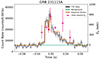 |
Fig. 1. Fermi/GBM light curve of GRB 231115A (black), binned at a temporal resolution of counts per 3 ms, with the background model (green). The brown line is the result of the BB analysis of the burst. The pink dots are the time-resolved peak energy values taken from Table 1. At this finer temporal resolution we see a double-peaked structure within the initial burst signal. |
The T90 duration, the interval between 5% and 95% of the cumulative fluence value, is T90 = 32 ± 36 ms. The time between which 25% and 75% of the total fluence was accumulated is T50 = 16 ± 23 ms. These values are determined by analyzing the background-subtracted light curve from the optimal detectors and fitting a Comptonized spectrum (see below) to track the fluence over time. Analyzing the event using BBs, we find a total burst duration (TBB) of 97 ms. The rise time of the initial peak is ∼ 2.7 ms. As in Roberts et al. (2021), we calculated the rise time of the pulse by fitting a pulse shape function and taking the elapsed time between the 10%–90% of the peak.
We analyzed the GBM data over energies ranging from 8 keV to 10 MeV for GRB 231115A and the KONUS data over energies ranging from 10 keV to 1.2 MeV for GRB 0511032. We also reanalyzed the data from GRB 180128A and GRB 200415A using asymmetric errors as they better capture the uncertainties inherent in Poisson-distributed measurements, providing a more accurate representation than symmetric errors used in the previous analyses. These new analyses involve both time-integrated and time-resolved spectral fits.
Both previously identified MGFs observed by Fermi/GBM were analyzed using the RMfit software3, which utilizes an adapted forward-folding Levenberg-Marquardt algorithm for spectral fitting (Goldstein et al. 2013). In this work, we instead employed the Nelder-Mead algorithm (Nelder & Mead 1965; Gao & Han 2012) for spectral fitting. While slower than Levenberg-Marquardt, Nelder-Mead provides a distinct advantage: if the true solution lies within the bounds of the initial simplex, convergence is guaranteed. This approach reduces the risk of becoming trapped in local minima. This is also a known limitation Levenberg-Marquardt.
While our findings are generally consistent with those reported in Roberts et al. (2021) and Trigg et al. (2024), some differences are apparent, reflecting the improved fitting procedure. These updates provide a more accurate and well-constrained data characterization, particularly for GRB 180128A, where the previous analysis encountered significant uncertainties.
We fit the differential energy spectrum for GRB 231115A to three different models. These models include a Band function (Band et al. 1993), a power-law function (PL), and a Comptonized function (COMPT; Gruber et al. 2014). COMPT exhibits a power-law behavior characterized by an index α, with an exponential cutoff at a characteristic energy Ep of the spectral peak of a νFν representation.
The three models were fit using the fit statistic pstat in GDT, which is a likelihood for Poisson data with assumed known background and is the same as the pstat statistic from the Xspec Statistics Appendix (Arnaud et al. 2011). Pstat was also used in the GBM spectral catalogs Gruber et al. (2014) and Poolakkil et al. (2021). We used the method in Gruber et al. (2014) to determine the best-fit model by comparing the ΔC-Stat (the difference in log-likelihood per degree of freedom) of the various models against the critical delta log-likelihood ΔC-Statcrit values listed in Gruber et al. (2014, see our Table D.1).
We performed time-integrated fits for the significant emission durations as defined by the BB analysis for the bursts. The results of these time-integrated fits, reported in Table 1, provide an overview of the spectral properties over the entire emission period. Based on the previously mentioned best-fit criteria, the time-integrated data are best-fit by the COMPT model (see Fig. 2). Additionally, we conducted time-resolved fits using two approaches. The first method robustly determines the intervals by detecting and modeling changes in the gamma-ray emission rate, allowing the capture of detailed spectral evolution. The second approach uses intervals with equal durations to provide a consistent comparison across different phases of the bursts. The preferred model is PL for one interval in the time-resolved equal duration fit and four intervals in the time-resolved BB duration fit. The PL model preferred over the COMPT model is likely due to photon counts being too low to statistically prefer the curvature constraints of the COMPT model for those durations. However, we assumed that the COMPT model is the more accurate spectral form based on the time-integrated analysis.
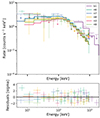 |
Fig. 2. Time-integrated spectral fit to a COMPT model for GRB 231115A. |
Time-resolved spectral analysis using BBs.
The results of the time-resolved fits, presented at the 90% confidence level, are listed in Tables 1 and B.1, highlighting the temporal variation in spectral properties for GRB 231115A and GRB 051103. Figure F.1 illustrates the fitted spectra of GRB 231115A corresponding to the data in Table 1. The derived values of α and Ep for both bursts are consistent with those of previously identified MGFs and MGF candidates (Burns et al. 2021; Trigg et al. 2024), with α typically ranging from approximately 0.0 to 1.0 and Ep spanning from ∼300 keV to several MeV. The analyses applied to the two previously identified extragalactic MGF candidates detected by Fermi/GBM, GRB 180128A and GRB 200415A, are summarized in Tables C.1 and B.1.
The Ep values from the time-resolved analysis in Table 1 exhibit variations comparable to those observed in GRB 200415A (Roberts et al. 2021) and GRB 180128A (Trigg et al. 2024). The significance of this variation is illustrated by the highlighted intervals in Fig. 3, which displays the 50% and 90% confidence intervals for the correlated parameters α and Ep. The statistical significance of the observed variations was evaluated to determine whether they represent genuine spectral evolution or are consistent with random fluctuations. We conducted a rigorous statistical analysis to evaluate the significance of the deviations in Ep values across the time-resolved BB intervals in Table 1. The time-integrated spectral fit, which provides a baseline of Ep = 600 ± 60 (90% confidence), was used as the reference for assessing the p-values for each BB interval. While multiple individual intervals showed deviations from the baseline value, we calculated a joint p-value to measure the collective significance of these deviations.
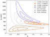 |
Fig. 3. Confidence contours for the time-resolved spectral analysis of GRB 231115A, corresponding to the BB intervals in Table 1. The contours represent the 50% and 90% confidence regions for the correlated parameters. Highlighted intervals illustrate spectral evolution within the burst. |
The joint p-value, obtained using Fisher’s combined probability test (Fisher 1970), aggregates the p-values of all the time-resolved intervals into a single statistic. This approach considers the overall pattern of deviations rather than treating each interval independently, making it particularly suited for evaluating trends in time-resolved spectral data. For GRB 231115A, the resulting joint p-value is 0.002, corresponding to 3σ significance. This low probability demonstrates that the observed evolution in Ep across the intervals is highly unlikely to result from random fluctuations, providing robust statistical confirmation of the spectral evolution.
2.2. Highest-energy photons
Figure 4 shows the individual TTE counts in GBM BGO detector 1. GBM cannot determine with certainty whether any particular event is from GRB 231115A, another gamma-ray source, or due to other background signals. We can assess whether a rate increase is statistically significant and thus likely associated with GRB 231115A, using a Bayesian algorithm over Poisson data as a classic on-source:off-source method of source detection. This method is described in detail in Roberts et al. (2021) for MGF, GRB 200415A. Over the 624 ms interval of our analysis, we find 110 TTE photons in a 576 ms background interval and 25 TTE photons in a 48 ms on-source window for energies ranging from 655 to 930 keV. The calculated probability for a source signal (GRB 231115A) above the background is 0.999905 (∼4σ), providing strong evidence that EMax is ∼ 930 keV. For clarity, Fig. 4 highlights a 140 ms window around T0 to better display the on-source interval.
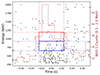 |
Fig. 4. Energetic photons from GRB 231115A. Individual TTEs of GBM BGO detector 1 are indicated with black dots. The blue rectangle highlights energies from 655 keV to 930 keV, and the red rectangle energies from 930 keV to 1192 keV. We conclude that the highest photon energy associated with GRB 231115A is ∼900 keV. |
We also considered a higher energy range, 930 to 1192 keV, for which there are 108 off-source TTE photons and nine on-source TTE photons (red box in Fig. 4). The probability that the 9 on-source TTE photons represent an excess rate attributable to GRB 231115A is 0.8545 (∼1.5σ), providing marginal evidence of the detection of EMax ∼ 1.1 MeV photons for GRB 231115A by GBM, which is nearly one-third the energy of the highest-energy photons observed for GRB 200415A (Roberts et al. 2021), and somewhat similar to that reported by WIND solid-state telescope silicon detectors for the 27 December 2004 MGF initial pulse of SGR 1806-20 (Boggs et al. 2007). We therefore conclude that the highest photon energy associated with GRB 231115A is ∼ 900 keV.
2.3. Minimum variability timescale
The minimum variability timescale (MVT) is a measure of the shortest duration of significant fluctuation in the light curve of a GRB. Typically ranging from milliseconds to seconds, these timescales indicate rapid changes in the flux or intensity of a GRB. Given that MGFs can have bulk Lorentz factors (Γ) that are several orders of magnitude smaller than cosmological GRBs, we expect the MVTs to be much shorter for MGFs. The Golkhou et al. (2015) method, based on Haar wavelets, yields an MVT of Tmin = 1.1 ± 0.7 ms for GRB 231115A. An independent calculation identifies the MVT as the shortest binning timescale where the GRB signal is distinguishable from background fluctuations (Bhat et al. 2011). This method produces a similar MVT value, Tmin = 1.1 ± 1.4 ms. While this value is unconstrained, the consistency between these two independently derived values strongly suggests that this is the true MVT for GRB 231115A, enhancing the reliability of our measurement and the robustness of our method. The rise time value (Sect. 2.1) is broadly consistent with the MVTs Trise = 2.7 ± 1.1 ms. These timescales correspond to an upper limit to the typical emission size, cT ≲ 3 × 10⁷ (T/ms) cm.
2.4. Quasi-periodic oscillations
We searched the NaI and BGO data separately for quasi-periodic oscillations (QPOs). First, we generated light curves with a time resolution of 0.122 ms, allowing us to search up to a frequency of 4096 Hz. We then created Leahy-normalized periodograms from those light curves and found that frequencies above 100 Hz are largely free of burst variability and thus consistent with white noise. We searched the frequency range from 100 to 4096 Hz using standard outlier detection techniques in the linearly and logarithmically binned periodograms and found no credible candidate detection at p < 0.01, corrected for the number of frequencies searched.
At frequencies below 100 Hz, we implemented the method described in Hübner et al. (2022) and fit a model to the light curve containing an overall burst envelope parameterized as a skewed Gaussian as well as a damped random walk stochastic process. We compared that model to one that also includes a QPO parameterized as a stochastically driven damped harmonic oscillator. We compared models using the Bayes factor and define a strong candidate as one where log10(ℬ) > 2. We find a Bayes factor of log10(ℬNaI) = 0.24 and log10(ℬBGO) = 0.49 for the NaI and BGO, respectively, and conclude that there is no credible QPO candidate present in the data.
3. Follow-up observations
Rapid follow-up observations provide a compelling case for GRB 231115A as an extragalactic MGF. Below we detail our additional results and analyses, which support the conclusions in Mereghetti et al. (2024).
3.1. X-ray
The arcminute localization uncertainty to GRB 231115A offers a rare opportunity to search for the X-ray counterpart. Here, we briefly discuss the alternatives for such a search, focusing on the capabilities of current satellites.
3.1.1. Persistent source
Magnetars are persistent soft X-ray emitters, with emission potentially involving a heterogeneous, hot thermal surface modified by a highly magnetized atmosphere (e.g., Viganò et al. 2013). Observations suggest a negative correlation between the surface temperature – and consequently soft X-ray luminosity – and the magnetar spin-down age within the population: younger magnetars are brighter and exhibit stronger bursting activity (e.g., Olausen & Kaspi 2014; Viganò et al. 2013; Enoto et al. 2019). The brightest magnetars have persistent luminosities of LX, per ≳ 1035 erg s−1. However, there is a maximum luminosity for magnetar soft thermal emission dictated by neutrino losses in the inner crust: LX, max ≲ 1036 erg s−1 (e.g., Pons & Rea 2012). This saturation restricts the detectability of such emissions from extragalactic magnetars at a distance of ≳3.5 Mpc.
The galaxy M82 has been observed with Chandra throughout the mission, accumulating a total exposure of approximately 1 Ms. The luminosity distribution of the Chandra point sources within a 4′ radius around the INTEGRAL burst position of GRB 231115A, including foreground and background sources unrelated to M82, is shown in Fig. 5 (light gray). These data are taken from the Chandra Source Catalog4 (CSC). For comparison, the distribution of the known magnetar population is shown (dark gray), though it is heavily biased toward the brighter and most active magnetars. The faintest source detected with Chandra has a luminosity of LX ≈ 1036 erg s−1, at the limit of the theoretical expectation for the maximum soft X-ray luminosity of a magnetar, though brighter by a factor of two than the brightest known magnetar (SGR 0526−66, LX ≈ 5 × 1035 erg s−1; Kulkarni et al. 2003; Park et al. 2012). While a few of these faint sources might be good magnetar candidates, without enough counts for an adequate spectral and, most importantly, temporal analysis, it is difficult to determine their true nature. Given the high star formation rate in M82, other possible source types include young pulsars, accreting pulsars, high-mass X-ray binaries, and young supernova remnants.
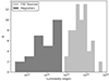 |
Fig. 5. Luminosity distribution of M82 Chandra point sources within the INTEGRAL uncertainty region of GRB 231115A (light gray histogram). They are detected in the full Chandra exposure of the galaxy, totaling ≈1 Ms. The dark gray histogram represents the luminosity distribution of known magnetars. |
3.1.2. Bursting magnetar
Given that all three confirmed MGFs were accompanied by short bursts occurring within hours to days following the event (Mazets et al. 1979; Woods et al. 1999; Frederiks et al. 2007a), we devised a methodology to blind-search for short bursts in imaging data such as XMM-Newton European Photon Imaging Camera (EPIC-PN) and NuSTAR focal plane modules (FPMs) as follows. We produced cleaned images in the 2–10 keV for PN and 3–70 keV ranges for FPMs, centered at the INTEGRAL localization ±4′. We searched consecutive one-second frames (with a 0.2 s overlap) within valid good-time intervals. For this search, we used the SAS tool edetect_chain5 for PN and the DETECT tool, part of the XIMAGE software for FPMs (Perri et al. 2013). Once these tools flag candidate sources, we compared their excess counts, n, to the local background rate, λ, determined from the full observation, and calculated the probability that the counts occur randomly, Pi = λnie−λ/ni!, where index i is for each frame searched. Frames with candidate sources having probability Pi < 0.01/N, where N is the number of frames searched (approximately equal to the live-time in each observation), are considered valid sources at the 99% confidence level (trial corrected). We find no source that meets our criteria for a confident detection in either XMM-Newton or NuSTAR.
We established the upper limit on the detectability of short bursts in these observations through simple simulations. We assumed that the magnetar short bursts’ light curves have a fast-rise exponential-decay shape, with rise and decay times of 0.5 ± 0.3 and 0.7 ± 0.3 seconds, respectively (e.g., Younes et al. 2020). We assumed the burst spectra to follow a two-blackbody model with temperatures of 5 and 11 keV (e.g., Lin et al. 2020). Finally, we varied the 1–100 keV burst energy between 1041 erg and 1043 erg logarithmically, in 20 steps. For each simulated burst, the estimated number of counts and their corresponding times and energies are injected into the actual XMM-Newton (or NuSTAR) event file, and our search methodology is repeated. As two extreme cases, we injected the simulated "source" at the edge of the INTEGRAL error circle, away from point sources, and at the galaxy’s bright center.
We find that the short burst fluence detection thresholds, according to our criterion, are ≳4 × 10⁻¹⁰ erg cm−2 and ≳10−9 erg cm−2 for the edge and center cases, respectively. This translates to 1–100 keV energies of approximately 6 × 1041 erg s−1 and 1.5 × 1042 erg s−1, respectively (Fig. 6). These figures are similar for XMM-Newton and NuSTAR, and are at the high end of typical short burst energetics, approaching the energies of intermediate flares.
 |
Fig. 6. Detectability of short bursts with XMM-Newton (black and gray lines) and NuSTAR (blue and cyan lines), if the putative magnetar is coincident with the center of the galaxy or offset by a few arcminutes, respectively. The vertical dotted lines correspond to burst energy for which a trial-corrected confidence level is 99% for each case. See the main text for more details. |
Due to the steep log N-log S distribution of bursts, our non-detection with PN and FPMs is not surprising. Better prospects can be achieved with the High Energy X-ray Probe (HEX-P; Madsen et al. 2019), yet still at the level of the brightest short magnetar bursts (Alford et al. 2024).
3.1.3. MGF tail detection
Currently, the combination of Swift’s Burst Alert Telescope (BAT; Barthelmy et al. 2005) and autonomous re-pointing to observe with the Swift/XRT is the most promising means by which to capture a MGF tail in time for a possible detection. Unfortunately, for the existing catalog of extragalactic MGF candidates, the source was outside the BAT coded field of view, preventing a possible BAT trigger and the seconds-scale automatic re-pointing of Swift. Another possible avenue is NICER’s new capability for automatic re-pointing via a MAXI trigger (OHMAN; Gendreau et al. 2023). However, this is limited by the low rate of short-GRB detection with MAXI, given its limited energy range 2 − 30 keV, and NICER visibility, which is complex due to the structure of the International Space Station.
To assess the detectability of MGF tails with Swift and a NICER-like instrument, we simulated the 2004 MGF tail from SGR 1806−20 as presented in Hurley et al. (2005, see also Palmer et al. 2005). The spectrum is modeled as a blackbody with a constant temperature of about 8 keV, folded through the response matrices and effective area curves of Swift/XRT and NICER. The decay follows the evaporating fireball model Lx(t) = L0[1 − (t/tevap)]a/(1 − a) with L0 = 1042 erg s−1 in the 20–100 keV energy range measured at t ≈ 40 s after the initial spike, tevap = 382 s, and a = 0.6 (Hurley et al. 2005). Finally, we modulated the decaying tail at a fiducial spin period of P = 5 s with a pulse shape following a Fourier series with two harmonics (having approximately equal power; see the inset of Fig. 7) and an rms pulsed fraction of 45%. An example light curve for Swift and NICER at the M82 distance of 3.5 Mpc is shown in the left panel of Fig. 7.
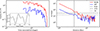 |
Fig. 7. Re-pointing simulation results. Left: Simulated MGF tail light curve with XRT (blue) and NICER (red) assuming the properties as observed in the SGR 1806−20 MGF tail, and scaling it to the M82 distance of 3.5 Mpc. The inset shows the modulation that is embedded in the light curve. Right: Z22 power for pulsation detection in XRT and NICER as a function of MGF distance. The dot-dashed and the dotted lines show the 4.5σ and 3σ detection significance (single-trial), respectively. The vertical dashed line is the M82 distance of 3.5 Mpc. See the main text for more details. |
The detectability of the tail at extragalactic distances will largely depend on the re-pointing time and the background rate of the instrument (Negro et al. 2024). The latter is ≈5 × 10⁻³ counts s−1 and ≈5 × 10⁻¹ counts s−1 for XRT and NICER in the energy range 0.5–10 keV, respectively. For each light curve, we derived the cumulative counts in the tail from a start time ranging from 40 to 300 seconds and compared them to the cumulative background counts in the same time interval. We find that a 3σ detection (based on a Poisson probability density function for XRT and a Gaussian probability density function for NICER) can be achieved for re-pointing times of ≲250 seconds for both instruments.
However, pulsation detection, shown in the right panel of Fig. 7 in the form of the Z22 power, is more prominent in NICER compared to XRT. Varying the distance from 1 Mpc to 20 Mpc reveals that a NICER-like instrument can detect the pulsations in the tail up to a distance of ∼6 Mpc, while an XRT-like instrument can do so up to 4 Mpc (Fig. 7, right panel). One caveat is that XRT needs to operate in windowed-timing mode to detect pulsations < 5 seconds due to its limited timing resolution of 2.5 seconds when operating in photon-counting mode.
Identifying the progenitor magnetar of an extragalactic MGF within a few megaparsecs hinges on detecting the X-ray tail, which requires a rapid, autonomous response from instruments such as XRT. XRT provides arcsecond localization, which is crucial for studying the magnetar environment - a challenge in the Milky Way due to higher column densities and uncertain distances to Galactic magnetars. The X-ray follow-up of triggers from other satellites is also critical; for example, XRT or NICER could have succeeded in an automated follow-up of an INTEGRAL event. While less probable, a detection by NICER through the OHMAN program could potentially represent the first observation of a pulse period from an extragalactic magnetar. With incremental improvements to currently available technology, the prospects for such detections could significantly improve, for example by utilizing detectors like the Low Energy Modular Array and the High Energy Modular Array on the proposed probe-class mission STROBE-X (Spectroscopic Time-Resolving Observatory for Broadband Energy X-rays; Ray et al. 2019).
3.2. Optical
Here, we present our optical follow-up with the 2.1m Fraunhofer telescope (Hopp et al. 2014) at Wendelstein Observatory, Germany.
Observations with the Three Channel Camera (3KK; Lang-Bardl et al. 2016) at Wendelstein Observatory began on 16 November 2023 at 00:39 UT in the riJH filters for two hours. Additional observations were performed on 22 November 2023 at 00:16 UT with the 3KK camera simultaneously in the riJ filters for one hour, and the Wendelstein Wide Field Imager (WWFI; Kosyra et al. 2014) in the g filter for one hour.
Data reduction was performed using a custom pipeline developed at the University Observatory Munich, for both the WWFI and 3KK cameras (Gössl & Riffeser 2002; Kluge 2020; Kluge et al. 2020). The pipeline corrects for bias, dark, and flat-field properties and detector artifacts. It uses SCAMP (Bertin 2006) to compute the astrometric solution with respect to the Gaia Early Data Release 3 catalog (Gaia Collaboration 2021), and SWarp (Bertin et al. 2002; Bertin 2010) to co-add images. Photometric zero points were calibrated using nearby stars in the Pan-STARRS-3 Pi (PV3; Magnier et al. 2013) source catalog and Two Micron All Sky Survey (2MASS; Skrutskie et al. 2006) catalog.
Difference imaging was conducted using the Saccadic fast Fourier transform algorithm6 (Hu et al. 2022). Archival templates from the WWFI, obtained in 2014 in g and r bands, were used as references. For other filters (i and J) we performed difference imaging between images acquired on 16 November 2023 and 22 November 2023. Our analysis did not reveal and confidently detect rapidly varying transients between epochs. The 5σ upper limits for each filter are reported in Table E.1.
4. Discussion
While the sky association of GRB 231115A with the nearby galaxy M82 is strongly suggestive of a non-cosmological GRB origin for this transient, its spectral evolutionary character provides additional localization-independent arguments for it being a MGF. This is predicated on similarities of its spectral evolution with those of the two MGFs from the Sculptor galaxy, NGC 253, namely GRB 180128A (Trigg et al. 2024) and GRB 200415A (Roberts et al. 2021). The character of this evolution is naturally expected for an intense radiation beam from a rotating magnetar, a model that was highlighted in Roberts et al. (2021). In the absence of an oscillatory tail (discussed in Sect. 3.1.3), the smoking gun signature of a MGF, the initial spike spectral evolution is the main information that can yield insights into the source of these transients.
The rotating, relativistic “lighthouse” picture presumes that the plasma that powers the MGF is blasted off the magnetar surface near the magnetic poles and escapes as a wind to high altitudes and beyond the magnetosphere (e.g., Thompson & Duncan 1995). This ejection could be triggered by the buildup of magnetic stresses in the crust that eventually force it to crack and release copious amounts of plasma and energy. The highly super-Eddington environment and enormous energy density forces the plasma to flow out at relativistic speeds. This expectation is commensurate with lower limits to the bulk Lorentz factor (Γ) of the outflow that is obtained from the argument that the emission region is transparent to γγ → e+e− pair creation for all photons up to the maximum energy, Emax observed. This transparency is aided by Doppler beaming of the radiation (Krolik & Pier 1991; Baring 1993), and Γ > Emax/511 keV is the most conservative bound possible. Transparency of the emission to two-photon pair creation up to Emax ∼ 900 keV (nearly double the threshold for pair creation) guarantees that the bulk Lorentz factor of the emitting plasma is at least around Γ ∼ 2 relative to the observer, which is less than Γ > 6 that Roberts et al. (2021) obtained for GRB 200415A, which had Emax ∼ 3 MeV. In contrast, GRB 180128A was somewhat fainter with no photons above 511 keV in energy and above the background level, so Γ > 1 is thereby unconstrained.
The deduced relativistic motion of the plasma automatically implies that the brightness of the flare will vary rapidly and be correlated with its spectral evolution in a fairly well-defined manner dictated by standard special relativistic transformations. As the radiation–plasma beam sweeps across the line of sight to Earth, the luminosity should first intensify and the spectrum should harden to higher energies, and then both should recede (soften) as the beam rotates away from the observer (Roberts et al. 2021). This is the evolutionary sequence seen in both MGF candidates, GRBs 180128A and GRB 200415A.
To illustrate that GRB 231115A exhibits the evolutionary sequence discussed in above, and verified statistically in Sect. 2.1, we plotted four of the BB intervals (the Ep values for all of the BB intervals are plotted in on the light curve in Fig. 1). The results, shown in Fig. 8, showcase the spectral evolution from the onset of the burst through the two peaks and into the brief emission that follows. For clarity, the third, sixth, and seventh BB intervals have been omitted from Fig. 8, although they align with the overall trend seen in the included intervals. This spectral evolution, characteristic of a MGF, is clearly apparent for GRB 231115A. Such “envelope” behavior is primarily a consequence of the Doppler beaming and boosting from the radiating plasma. This behavior does not naturally arise for classical GRBs born from collapsars or neutron star-neutron star mergers, and so one can conclude that GRB 231115A is likely the initial spike of a MGF.
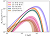 |
Fig. 8. Spectra of GRB 231115A over four BB time intervals. The intervals show the onset of the burst (1), peak 1 (2), peak 2 (4), and the extended emission after the peaks (5). Intervals (3), (6), and (7) are omitted for clarity but are consistent with the trend displayed. The shaded area indicates the 90% confidence regions. |
The Δt ∼ 40 ms timescale for the overall evolution in Fig. 9 can be used to provide a lower bound to the magnetar’s rotation period. This time corresponds to a stellar rotation through an angle Δθ ∼ 2πΔt/P for a rotation period of P. For a rotating beam of relativistic plasma, the peak flux of the emission light curve will be approximately confined to the Doppler cone of opening angle 1/Γ, as long as the angular extent of the wind’s collimation is not large. Combining these, one estimates that the putative neutron star’s spin period should be bounded by P ∼ 2πΓ Δt ≳ 500 ms for Γ > 2 for GRB 231115A. In practice, the bulk motion is expected to be somewhat or significantly faster than the pair creation transparency bound suggests. This is mainly due to the plasma dynamics associated with the large amount of energy deposited into the inner magnetosphere over short timescales. It is notable that the detection of delayed GeV-band emission in association with the GRB 200415A giant flare suggested that Γ ∼ 100 was likely (Ajello et al. 2021). If Γ lies in the 3 − 50 range for GRB 231115A, then the deduced period P would be commensurate with those of Galactic magnetars.
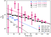 |
Fig. 9. Comptonized spectrum peak energy (Ep) as a function of time using a temporal binning of 8 ms and values from Table B.1. All fit errors and error bars are at the 90% confidence level. The zero-time reflects the GBM event start time of each detection. |
Nonuniformity of the expanding wind naturally yields fluctuations in the Doppler elements, and these are reflected in both the light curve, which has a flux (luminosity) tracer Liso, and the spectroscopy, for which we used Ep as a hardness marker. In Fig. 10 we illustrate that these two quantities are fairly tightly correlated for GRB 231115A and prior MGFs approximately via the  form listed in Eq. (A.3). Roberts et al. (2021) emphasized that theoretically, the index β should be tightly coupled to the dual relativistic elements of Doppler boosting (influencing Ep ∝ Γ) and Doppler beaming (enhancing Liso). As was detailed in Trigg et al. (2024), the actual value of the index β should depend on the temporal sampling of the light curve, ranging from β ∼ 2 for approximately uniform time bins (see Fig. 10a), to β ∼ 4 for BB time intervals (see Fig. 10b)7. The physical origin of these two extremes is linked to the size of the look-back surface within the relativistic wind that is sampled during the time intervals. The BB choice yields partial samplings of smaller surface sizes that capture more of the Doppler flux beaming character Liso ∝ Γ4. Performing spectroscopy on uniform time bin selections tends to smear out the surface solid angle sampling fluctuations, emphasizing the photon energy boosting and time dilation characteristics, generating Liso ∝ Γ2 (Trigg et al. 2024). For GRB 231115A, the reality is between these two extremes, as it is for the other MGFs addressed in Fig. 10 and discussed in Trigg et al. (2024). Yet the fact that a steeper Liso − Ep correlation is evinced for the BB choice does indicate that the physical angular extent of the wind is modest or small, commensurate with expectations of a wind anchored to open field lines emerging from the magnetar’s polar surface.
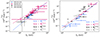 |
Fig. 10. Liso–Ep relation using different timing intervals. Left: Correlation between Liso and Ep for the four MGF candidates, GRB 231115A (light blue), GRB 051103 (pink), GRB 200415A (black), and GRB 180128A (gray), revealing an approximate |

Based on the saturation limit discussed in Sect. 3.1.1, the prospect of detecting the persistent emission from a magnetar following a MGF, whether during quiescence or an outburst, is slim at distances ≳3.5 Mpc. This situation slightly improves with the next-generation X-ray telescopes. For instance, the sensitivity limit for AXIS, a NASA Probe mission selected for Phase A (Reynolds et al. 2023), is about one to two orders of magnitude lower than Chandra’s, depending on the spectral shape of the underlying source population, a 250 ks exposure with AXIS reaches a limit of ≈10−16 erg s−1 cm−2 for a 5σ detection, which translates to 1035 erg s−1 at 3.5 Mpc (Safi-Harb et al. 2023). The prospect of identifying the magnetar, through either spectral or temporal analyses, is better for nearer galaxies such as Andromeda or M33. However, this limited volume constrains the number density of MGFs. It is clear that identifying the persistent counterpart to a candidate extragalactic MGF (in either quiescence or outburst) will require missions like AXIS and flagship X-ray missions such as Lynx or Athena; the launch of Athena is planned for late 2030. Additionally, an intentionally developed IPN could achieve arcsecond localization directly from the event spike.
Turning to the radio observations, the constraints mentioned in Sect. 1 are highly restrictive, with limits ranging from < 10−11 to 10−9 in radio-to-gamma-ray fluence given a flat radio spectral index and band extent of approximately a few times 108 Hz. It remains uncertain whether MGFs can produce prompt FRBs, as the statistics of FRBs resemble those of short bursts rather than MGFs (although shock models favor MGFs; see Popov & Postnov 2010; Lyubarsky 2014; Beloborodov 2017; Metzger et al. 2019). FRB(s) associated with the SGR 1806–20 MGF in 2004 would have been detected by Murriyang (Tendulkar et al. 2016), suggesting that MGFs do not generically result in FRBs. However, from the limited Galactic examples available, MGFs occur during active states of the magnetar, often coinciding with numerous short bursts. Therefore, FRBs could potentially be correlated with MGFs, though not directly caused by them (Ridnaia et al. 2024). Patchy observations from 2020-2022 searching for FRBs in M82 yielded limits of 1.2 × 1028 erg s−1 Hz−1 (Paine et al. 2024).
5. Conclusion
The detection and analysis of GRB 231115A provide compelling evidence that it is an extragalactic MGF originating from the starburst galaxy M82. This burst gives a fully self-consistent picture based on the model discussed in Sect. 4. The observed spectral evolution closely mirrors the characteristics of known MGFs from other galaxies, such as NGC 253, supporting the classification of GRB 231115A as a MGF. The comprehensive gamma-ray analysis conducted with Fermi/GBM data provides us with significant insights into the burst’s properties, including its high peak energy and complex temporal structure. The association of GRB 231115A with M82 is further strengthened by the high Bayes factor, suggesting a very low probability of a chance alignment with a cosmological neutron star merger.
The detection of high-energy photons at twice the threshold for γγ pair creation confirms a lower limit on the bulk Lorentz factor (Γ ≳ 2) of the outflowing plasma, consistent with expectations for relativistic winds from magnetars, and is comparable to observations from previous MGFs such as GRB 200415A and GRB 180128A. Moreover, the MVT indicates rapid flux changes typical of MGFs. This short timescale aligns with the smaller Lorentz factors expected for MGFs compared to cosmological GRBs, further supporting our classification.
This discovery not only adds to the growing list of extragalactic MGF candidates but also emphasizes the importance of prompt and coordinated multiwavelength follow-up observations for understanding these rare and energetic events. The ability to detect and accurately localize such MGFs in distant galaxies opens up new avenues for studying magnetars and their environments outside our Galaxy. The detectability of MGF tails at extragalactic distances is crucial, as they provide unambiguous evidence of magnetar central engines. Simulations show that the detectability of the tail depends significantly on the re-pointing time and instrument background rates. The limitations in detecting and characterizing MGFs with current instruments underscore the importance of new technologies and coordinated multiwavelength observations. Proposed missions and next-generation X-ray satellites are critical for advancing our understanding of these phenomena.
The detection of GRB 231115A and its unambiguous localization to M82 underscores the contribution of MGFs to the population of short GRBs. Future advancements in observational technology and methodologies, such as rapid automated re-pointing and increased X-ray sensitivity, will likely enhance our capacity to identify and study these phenomena, thereby furthering our understanding of the mechanisms driving short GRBs and the role of magnetars in the cosmos.
This analysis complements that of Frederiks et al. (2007b) and Svinkin et al. (2021), utilizing a different temporal binning.
The spectral analysis tool RMfit was initially designed for time-resolved analysis of BATSE GRB data. However, it has been adapted for GBM and other instruments supporting compatible FITS data formats. Information on the software can be accessed through the Fermi Science Support Center at https://fermi.gsfc.nasa.gov/ssc/data/p7rep/analysis/rmfit/
A detailed description of our fitting method can be found in Appendix A.
Acknowledgments
We thank the reviewer for their insightful comments and suggestions that significantly improved the quality of this manuscript. AT, EB, MN, and OJR acknowledge NASA support under award 80NSSC21K2038. MGB thanks NASA for support under grants 80NSSC22K0777 and 80NSSC22K1576. Z.W. acknowledges support by NASA under award number 80GSFC21M0002. The USRA coauthors gratefully acknowledge NASA funding through cooperative agreement 80NSSC24M0035. BO is supported by the McWilliams Postdoctoral Fellowship at Carnegie Mellon University. This paper contains data obtained at the Wendelstein Observatory of the Ludwig-Maximilians University Munich. The authors greatly acknowledge the assistance of the observer Michael Schmidt (USM) in obtaining the observations. This work was in part funded by the Deutsche Forschungsgemeinschaft (DFG, German Research Foundation) under Germany’s Excellence Strategy - EXC-2094 - 390783311. The work of DF and DS was supported by the basic funding program of the Ioffe Institute FFUG-2024-0002.
References
- Abadie, J., Abbott, B. P., Abbott, T. D., et al. 2012, ApJ, 755, 2 [NASA ADS] [CrossRef] [Google Scholar]
- Abbott, B. P., Abbott, R., Abbott, T. D., et al. 2017a, Phys. Rev. Lett., 118, 221101 [CrossRef] [Google Scholar]
- Abbott, B. P., Abbott, R., Abbott, T. D., et al. 2017b, Phys. Rev. Lett., 119, 141101 [CrossRef] [Google Scholar]
- Ajello, M., Atwood, W. B., Axelsson, M., et al. 2021, Nat. Astron., 5, 385 [CrossRef] [Google Scholar]
- Alford, J. A. J., Younes, G. A., Wadiasingh, Z., et al. 2024, Front. Astron. Space Sci., 10, 1294449 [NASA ADS] [CrossRef] [Google Scholar]
- Aptekar, R. L., Frederiks, D. D., Golenetskii, S. V., et al. 1995, Space Sci. Rev., 71, 265 [NASA ADS] [CrossRef] [Google Scholar]
- Arnaud, K., Smith, R., & Siemiginowska, A. 2011, Handbook of X-ray Astronomy (Cambridge University Press) [CrossRef] [Google Scholar]
- Band, D., Matteson, J., Ford, L., et al. 1993, ApJ, 413, 281 [Google Scholar]
- Baring, M. G. 1993, ApJ, 418, 391 [Google Scholar]
- Barthelmy, S. D., Barbier, L. M., Cummings, J. R., et al. 2005, Space Sci. Rev., 120, 143 [Google Scholar]
- Beloborodov, A. M. 2017, ApJ, 843, L26 [NASA ADS] [CrossRef] [Google Scholar]
- Bertin, E. 2006, in Astronomical Data Analysis Software and Systems XV, eds. C. Gabriel, C. Arviset, D. Ponz, & S. Enrique, ASP Conf. Ser., 351, 112 [Google Scholar]
- Bertin, E. 2010, SWarp: Resampling and Co-adding FITS ImagesTogether, Astrophysics Source Code Library [record ascl:1010.068] [Google Scholar]
- Bertin, E., Mellier, Y., Radovich, M., et al. 2002, in Astronomical Data Analysis Software and Systems XI, eds. D. A. Bohlender, D. Durand, & T. H. Handley, ASP Conf. Ser., 281, 228 [NASA ADS] [Google Scholar]
- Bhat, P. N., Briggs, M. S., Connaughton, V., et al. 2011, ApJ, 744, 141 [Google Scholar]
- Bingham, E., Chen, J. P., Jankowiak, M., et al. 2019, J. Mach. Learn. Res., 20(28), 1 [Google Scholar]
- Boggs, S. E., Zoglauer, A., Bellm, E., et al. 2007, ApJ, 661, 458 [NASA ADS] [CrossRef] [Google Scholar]
- Burns, E., Svinkin, D., Hurley, K., et al. 2021, ApJ, 907, L28 [NASA ADS] [CrossRef] [Google Scholar]
- Burrows, D. N., Hill, J. E., Nousek, J. A., et al. 2000, in X-Ray and Gamma-Ray Instrumentation for Astronomy XI (SPIE), 4140, 64 [NASA ADS] [CrossRef] [Google Scholar]
- Chen, T. W., Lin, C. S., Levan, A. J., et al. 2023, GRB Coordinates Network, 35052, 1 [NASA ADS] [Google Scholar]
- Cheung, C. C., Kerr, M., Grove, J. E., et al. 2023, GRB Coordinates Network, 35045, 1 [NASA ADS] [Google Scholar]
- CHIME/FRB Collaboration (Amiri, M., et al.) 2021, ApJS, 257, 59 [NASA ADS] [CrossRef] [Google Scholar]
- Curtin, A. P., & Chime/FRB Collaboration 2023, GRB Coordinates Network, 35070, 1 [NASA ADS] [Google Scholar]
- Dalessi, S., Roberts, O. J., Veres, P., Meegan, C., & Fermi Gamma-ray Burst Monitor Team 2023, GRB Coordinates Network, 35044, 1 [NASA ADS] [Google Scholar]
- D’Avanzo, P., Reguitti, A., Tomasella, L., et al. 2023, GRB Coordinates Network, 35077, 1 [Google Scholar]
- Duncan, R. C. 2001, in 20th Texas Symposium on relativistic astrophysics, eds. J. C. Wheeler, & H. Martel (AIP), AIP Conf. Ser., 586, 495 [CrossRef] [Google Scholar]
- Duncan, R. C., & Thompson, C. 1992, ApJ, 392, L9 [Google Scholar]
- Eichler, D., Livio, M., Piran, T., & Schramm, D. N. 1989, Nature, 340, 126 [NASA ADS] [CrossRef] [Google Scholar]
- Enoto, T., Kisaka, S., & Shibata, S. 2019, Rep. Prog. Phys., 82, 106901 [NASA ADS] [CrossRef] [Google Scholar]
- Fenimore, E. E., Klebesadel, R. W., & Laros, J. G. 1996, ApJ, 460, 964 [NASA ADS] [CrossRef] [Google Scholar]
- Fernández, C., & Steel, M. F. J. 1998, J. Am. Stat. Assoc., 93, 359 [Google Scholar]
- Feroci, M., Frontera, F., Costa, E., et al. 1999, ApJ, 515, L9 [Google Scholar]
- Fisher, R. A. 1970, Breakthroughs in statistics: Methodology and distribution (Springer), 66 [Google Scholar]
- Fong, W., Berger, E., Margutti, R., & Zauderer, B. A. 2015, ApJ, 815, 102 [NASA ADS] [CrossRef] [Google Scholar]
- Frederiks, D. D., Golenetskii, S. V., Palshin, V. D., et al. 2007a, Astron. Lett., 33, 1 [NASA ADS] [CrossRef] [Google Scholar]
- Frederiks, D. D., Palshin, V. D., Aptekar, R. L., et al. 2007b, Astron. Lett., 33, 19 [Google Scholar]
- Frederiks, D., Svinkin, D., Lysenko, A., et al. 2023, GRB Coordinates Network, 35062, 1 [NASA ADS] [Google Scholar]
- Gaia Collaboration (Brown, A. G. A., et al.) 2021, A&A, 649, A1 [NASA ADS] [CrossRef] [EDP Sciences] [Google Scholar]
- Gao, F., & Han, L. 2012, Comput. Optim. Appl., 51, 259 [CrossRef] [Google Scholar]
- Gendreau, K., Arzoumanian, Z., Mihara, T., et al. 2023, AAS/High Energy Astrophysics Division, 55, 111.01 [Google Scholar]
- Goldstein, A., Preece, R. D., Mallozzi, R. S., et al. 2013, ApJS, 208, 21 [Google Scholar]
- Goldstein, A., Veres, P., Burns, E., et al. 2017, ApJ, 848, L14 [CrossRef] [Google Scholar]
- Goldstein, A., Cleveland, W. H., & Kocevski, D. 2023, Fermi Gamma-ray Data Tools: v2.0.0, https://github.com/USRA-STI/gdt-fermi [Google Scholar]
- Golkhou, V. Z., Butler, N. R., & Littlejohns, O. M. 2015, ApJ, 811, 93 [NASA ADS] [CrossRef] [Google Scholar]
- Gössl, C. A., & Riffeser, A. 2002, A&A, 381, 1095 [NASA ADS] [CrossRef] [EDP Sciences] [Google Scholar]
- Grove, J. E., Cheung, C. C., Kerr, M., et al. 2020, Yamada Conference LXXI: Gamma-ray Bursts in the Gravitational Wave Era 2019, eds. T. Sakamoto, M. Serino & S. Sugta, http://yokohamagrb2019.wikidot.com/proceedings, 57 [Google Scholar]
- Gruber, D., Goldstein, A., von Ahlefeld, V. W., et al. 2014, ApJS, 211, 12 [Google Scholar]
- Hayatsu, S., Higuchi, N., Takahashi, I., et al. 2023, GRB Coordinates Network, 35057, 1 [NASA ADS] [Google Scholar]
- Homan, M. D., & Gelman, A. 2014, J. Mach. Learn. Res., 15, 1593 [Google Scholar]
- Hopp, U., Bender, R., Grupp, F., et al. 2014, in Ground-based and Airborne Telescopes V, eds. L. M. Stepp, R. Gilmozzi, & H. J. Hall, SPIE Conf. Ser., 9145, 91452D [NASA ADS] [Google Scholar]
- Hu, L., Wang, L., Chen, X., & Yang, J. 2022, ApJ, 936, 157 [NASA ADS] [CrossRef] [Google Scholar]
- Hu, L., Busmann, M., Gruen, D., et al. 2023, GRB Coordinates Network, 35092, 1 [NASA ADS] [Google Scholar]
- Hübner, M., Huppenkothen, D., Lasky, P. D., et al. 2022, ApJ, 936, 17 [Google Scholar]
- Hurley, K. 2011, Adv. Space Res., 47, 1337 [Google Scholar]
- Hurley, K., Cline, T., Mazets, E., et al. 1999, Nature, 397, 41 [NASA ADS] [CrossRef] [Google Scholar]
- Hurley, K., Boggs, S. E., Smith, D. M., et al. 2005, Nature, 434, 1098 [NASA ADS] [CrossRef] [Google Scholar]
- Hurley, K., Rowlinson, A., Bellm, E., et al. 2010, MNRAS, 403, 342 [CrossRef] [Google Scholar]
- Iskandar, A., Wang, F., Zhu, J., et al. 2023, GRB Coordinates Network, 35051, 1 [NASA ADS] [Google Scholar]
- Jiang, S. Q., Liu, X., Fu, S. Y., et al. 2023, GRB Coordinates Network, 35056, 1 [NASA ADS] [Google Scholar]
- Kaspi, V. M., & Beloborodov, A. M. 2017, ARA&A, 55, 261 [Google Scholar]
- Klebesadel, R. W., Strong, I. B., & Olson, R. A. 1973, ApJ, 182, L85 [NASA ADS] [CrossRef] [Google Scholar]
- Kluge, M. 2020, Ph.D. Thesis, Ludwig-Maximilians University ofMunich, Germany [Google Scholar]
- Kluge, M., Neureiter, B., Riffeser, A., et al. 2020, ApJS, 247, 43 [Google Scholar]
- Kosyra, R., Gössl, C., Hopp, U., et al. 2014, Exp. Astron., 38, 213 [NASA ADS] [CrossRef] [Google Scholar]
- Kouveliotou, C., Meegan, C. A., Fishman, G. J., et al. 1993, ApJ, 413, L101 [NASA ADS] [CrossRef] [Google Scholar]
- Kouveliotou, C., Wijers, R. A., & Woosley, S. 2012, Gamma-ray Bursts, 51 (Cambridge University Press) [CrossRef] [Google Scholar]
- Krolik, J. H., & Pier, E. A. 1991, ApJ, 373, 277 [NASA ADS] [CrossRef] [Google Scholar]
- Kulkarni, S. R., Kaplan, D. L., Marshall, H. L., et al. 2003, ApJ, 585, 948 [CrossRef] [Google Scholar]
- Kumar, R., Karambelkar, V., Swain, V., et al. 2023, GRB Coordinates Network, 35055, 1 [NASA ADS] [Google Scholar]
- Lang-Bardl, F., Bender, R., Goessl, C., et al. 2016, in Ground-based and Airborne Instrumentation for Astronomy VI, eds. C. J. Evans, L. Simard, & H. Takami, SPIE Conf. Ser., 9908, 990844 [NASA ADS] [Google Scholar]
- Ligo Scientific Collaboration, VIRGO Collaboration,& Kagra Collaboration 2023, GRB Coordinates Network, 35049, 1 [Google Scholar]
- Lin, L., Göğüş, E., Roberts, O. J., et al. 2020, ApJ, 902, L43 [NASA ADS] [CrossRef] [Google Scholar]
- Lyubarsky, Y. 2014, MNRAS, 442, L9 [Google Scholar]
- Madsen, K., Hickox, R., Bachetti, M., et al. 2019, BAAS, 51, 7 [NASA ADS] [Google Scholar]
- Magnier, E. A., Schlafly, E., Finkbeiner, D., et al. 2013, ApJS, 205, 20 [Google Scholar]
- Mazets, E. P., Golentskii, S. V., Ilinskii, V. N., Aptekar, R. L., & Guryan, I. A. 1979, Nature, 282, 587 [NASA ADS] [CrossRef] [Google Scholar]
- Mazets, E. P., Golenetskii, S. V., Gurian, I. A., & Ilinskii, V. N. 1982, Ap&SS, 84, 173 [NASA ADS] [CrossRef] [Google Scholar]
- Mazets, E. P., Aptekar, R. L., Cline, T. L., et al. 2008, ApJ, 680, 545 [Google Scholar]
- Meegan, C., Lichti, G., Bhat, P., et al. 2009, ApJ, 702, 791 [NASA ADS] [CrossRef] [Google Scholar]
- Mereghetti, S., Gotz, D., Ferrigno, C., et al. 2023, GRB Coordinates Network, 35037, 1 [NASA ADS] [Google Scholar]
- Mereghetti, S., Rigoselli, M., Salvaterra, R., et al. 2024, Nature, 629, 58 [NASA ADS] [CrossRef] [Google Scholar]
- Metzger, B. D., Margalit, B., & Sironi, L. 2019, MNRAS, 485, 4091 [NASA ADS] [CrossRef] [Google Scholar]
- Minaev, P. Y., Pozanenko, A. S., Grebenev, S. A., et al. 2024, Astron. Lett., 50, 1 [Google Scholar]
- Nakar, E. 2007, Phys. Rep., 442, 166 [NASA ADS] [CrossRef] [Google Scholar]
- Negro, M., Younes, G., Wadiasingh, Z., et al. 2024, Front. Astron. Space Sci., 11, 1388953 [NASA ADS] [CrossRef] [Google Scholar]
- Nelder, J. A., & Mead, R. 1965, Comput. J., 7, 308 [Google Scholar]
- Ofek, E. O., Kulkarni, S., Nakar, E., et al. 2006, ApJ, 652, 507 [Google Scholar]
- Ofek, E. O., Muno, M., Quimby, R., et al. 2008, ApJ, 681, 1464 [Google Scholar]
- Olausen, S. A., & Kaspi, V. M. 2014, ApJS, 212, 6 [Google Scholar]
- Osborne, J. P., Sbarufatti, B., D’Ai, A., et al. 2023, GRB Coordinates Network, 35064, 1 [NASA ADS] [Google Scholar]
- Paine, S., Hawkins, T., Lorimer, D. R., et al. 2024, MNRAS, 528, 6340 [NASA ADS] [CrossRef] [Google Scholar]
- Palmer, D. M., Barthelmy, S., Gehrels, N., et al. 2005, Nature, 434, 1107 [NASA ADS] [CrossRef] [Google Scholar]
- Park, S., Hughes, J. P., Slane, P. O., et al. 2012, ApJ, 748, 117 [NASA ADS] [CrossRef] [Google Scholar]
- Perley, D. A., Hinds, K. R., Wise, J., et al. 2023, GRB Coordinates Network, 35067, 1 [NASA ADS] [Google Scholar]
- Perri, M., Puccetti, S., Spagnuolo, N., et al. 2013, The NuSTAR data analysis software guide, https://heasarc.gsfc.nasa.gov/docs/nustar/analysis/nustar_swguide.pdf [Google Scholar]
- Phan, D., Pradhan, N., & Jankowiak, M. 2019, arXiv e-prints [arXiv:1912.11554] [Google Scholar]
- Pons, J. A., & Rea, N. 2012, ApJ, 750, L6 [NASA ADS] [CrossRef] [Google Scholar]
- Poolakkil, S., Preece, R., Fletcher, C., et al. 2021, ApJ, 913, 60 [NASA ADS] [CrossRef] [Google Scholar]
- Popov, S. B., & Postnov, K. A. 2010, in Evolution of Cosmic Objects through their Physical Activity, eds. H. A. Harutyunian, A. M. Mickaelian, & Y. Terzian, 129 [Google Scholar]
- Rastinejad, J. C., Gompertz, B. P., Levan, A. J., et al. 2022, Nature, 612, 223 [NASA ADS] [CrossRef] [Google Scholar]
- Ray, P., Arzoumanian, Z., Ballantyne, D., et al. 2019, BAAS, 51, 231 [NASA ADS] [Google Scholar]
- Reynolds, C. S., Kara, E. A., Mushotzky, R. F., et al. 2023, in UV, X-Ray, and Gamma-Ray Space Instrumentation for Astronomy XXIII, eds. O. H. Siegmund, & K. Hoadley, Int. Soc. Opt. Photon. (SPIE), 12678, 126781E [Google Scholar]
- Ridnaia, A., Frederiks, D., & Svinkin, D. 2024, MNRAS, 527, 5580 [Google Scholar]
- Rigoselli, M., Pacholski, D. P., Mereghetti, S., Salvaterra, R., & Campana, S. 2023, GRB Coordinates Network, 35175, 1 [NASA ADS] [Google Scholar]
- Roberts, O. J., Veres, P., Baring, M. G., et al. 2021, Nature, 589, 207 [NASA ADS] [CrossRef] [Google Scholar]
- Safi-Harb, S., Burdge, K. B., Bodaghee, A., et al. 2023, arXiv e-prints [arXiv:2311.07673] [Google Scholar]
- Scargle, J. D., Norris, J. P., Jackson, B., & Chiang, J. 2013, ApJ, 764, 167 [Google Scholar]
- Skrutskie, M. F., Cutri, R. M., Stiening, R., et al. 2006, AJ, 131, 1163 [NASA ADS] [CrossRef] [Google Scholar]
- Svinkin, D., Frederiks, D., Hurley, K., et al. 2021, Nature, 589, 211 [NASA ADS] [CrossRef] [Google Scholar]
- Tendulkar, S. P., Kaspi, V. M., & Patel, C. 2016, ApJ, 827, 59 [NASA ADS] [CrossRef] [Google Scholar]
- Thompson, C., & Duncan, R. C. 1995, MNRAS, 275, 255 [Google Scholar]
- Trigg, A. C., Burns, E., Roberts, O. J., et al. 2024, A&A, 687, A173 [NASA ADS] [CrossRef] [EDP Sciences] [Google Scholar]
- Troja, E., Fryer, C. L., O’Connor, B., et al. 2022, Nature, 612, 228 [NASA ADS] [CrossRef] [Google Scholar]
- Turpin, D., Thuillot, W., Souami, D., et al. 2023, GRB Coordinates Network, 35078, 1 [NASA ADS] [Google Scholar]
- Veres, P., Bhat, P. N., Burns, E., et al. 2023, ApJ, 954, L5 [NASA ADS] [CrossRef] [Google Scholar]
- Viganò, D., Rea, N., Pons, J. A., et al. 2013, MNRAS, 434, 123 [CrossRef] [Google Scholar]
- von Kienlin, A., Meegan, C. A., Paciesas, W. S., et al. 2020, ApJ, 893, 46 [Google Scholar]
- Woods, P. M., Kouveliotou, C., van Paradijs, J., et al. 1999, ApJ, 524, L55 [CrossRef] [Google Scholar]
- Woosley, S., & Bloom, J. 2006, ARA&A, 44, 507 [NASA ADS] [CrossRef] [Google Scholar]
- Xue, W. C., Xiong, S. L., Li, X. B., Li, C. K., & Insight-HXMT Team 2023, GRB Coordinates Network, 35060, 1 [NASA ADS] [Google Scholar]
- Younes, G., Güver, T., Kouveliotou, C., et al. 2020, ApJ, 904, L21 [CrossRef] [Google Scholar]
- Zhang, S.-N., Li, T., Lu, F., et al. 2020, Sci. China Phys. Mech. Astron., 63, 249502 [NASA ADS] [CrossRef] [Google Scholar]
Appendix A: Liso–Ep relation fitting method
In previous analyses of the luminosity-hardness correlation relationship between Liso and Ep, such as those in Roberts et al. (2021) and Trigg et al. (2024), data fitting used the assumptions of symmetric errors for the dependent (Liso) and independent variables (Ep), sometimes even ignoring the errors in the Ep entirely, as is common in least-squares regression. To better constrain the fit values for the Liso–Ep relation of GRB 231115A and GRB 051103, as well as reevaluate GRB 200415A, and GRB 180128A, we used statistical methods that account for asymmetric errors in both variables. This method allows the unbiased determination of probability distributions for the model parameters of interest.
Errors on both Ep and Liso are heteroscedastic (different for each data point) and asymmetric. To model the asymmetric errors in each dimension, we used a two-piece normal (TPN) distribution as proposed by Fernández & Steel (1998). This distribution corresponds to two half-normal distributions with standard deviations σ1 (left-hand side) and σ2 (right-hand side), joined at a common mode μ and renormalized such that the distribution is continuous. This distribution is usually parametrized by a common standard deviation σ and a skewness λ, with the probability density then being
 (A.1)
(A.1)
where
 (A.2)
(A.2)
These two equations enable the straightforward conversion of asymmetric errors as reported in the astronomical literature into a single standard deviation and skewness for use with the TPN.
To account for the presence of errors in both variables, we built an errors-in-variables model. Our data consists of pairs of observed values {Ep*, Liso*}. We assumed that the observed Ep* are random variables drawn from a TPN distribution with a mean given by a set of unknown true  values. To identify the luminosity-hardness correlation, we assumed a standard power-law relationship between the variables of the form
 (A.3)
(A.3)
We note that this relationship holds between the (unknown) true peak energy and isotropic luminosity, not the observed quantities. Whereas a standard likelihood assumes that the  are known, the errors-in-variables model infers them along with the parameters of the relationship, such that the total number of parameters to be inferred becomes
  , for N data points, a power-law amplitude α and a power-law index β. We infer the parameters in a Bayesian framework:
 (A.4)
(A.4)
Intuitively, this model parametrizes the data generation process: a power-law relationship exists between the unknown true peak energies and the unknown true isotropic luminosities. We first parametrized the relationship between the true peak energies and observed peak energies using the TPN distribution, and drew from it as well as the priors for the other parameters α and β. We can assume conditional independence and as such the priors for all parameters can be written independently:

The observed isotropic luminosities are then governed by a power-law relationship between the sampled true  and true, unknown
  , given parameters α and β, and compared to the observed Liso* through a likelihood
  , where σL and λL are the standard deviation and skewness for Liso* as defined using Eq. A.2.
This model can be sampled with Markov chain Monte Carlo in order to infer the true  and the power-law parameters α and β. To do so, one first samples
  from a prior distribution, and then computes a likelihood
  for the observed peak energy given the true peak energy using the TPN distribution. In a second step, the
  values are used to compute the proposed power-law relationship, together with α and β, also sampled from a prior. This relationship is then compared to the observed Liso*, again using a TPN distribution to obtain the posterior probability for the parameters. This model enables us to effectively take into account the asymmetric uncertainties on both peak energy and isotropic luminosity.
We set uninformative, flat priors on all parameters, where the prior for peak energies are defined as  , the prior on the power-law index is β ∼ 𝒰(1, 4) and the prior on the natural logarithm of the amplitude is log(α)∼𝒰(−2, 4), where 𝒰(a, b) denotes a uniform distribution between lower boundary a and upper boundary b.
We implemented the model in the probabilistic programming language numpyro (Phan et al. 2019; Bingham et al. 2019) and used Hamiltonian Monte Carlo with the No U-Turn Sampler (NUTS; Homan & Gelman 2014) to sample the posteriors for all parameters. We ran six Hamiltonian Monte Carlo chains with 4,000 warmup steps and 10,000 sampling steps. We assessed convergence using autocorrelation time and the Gelman-Rubin statistic and find that all chains are well converged (TGR ≤ 1.001 for all parameters).
Figure A.1 shows the results of the modeling for GRB 200415A. We chose this burst as it has good count statistics and the luminosity-hardness correlation has been derived by several previous studies (Roberts et al. 2021; Trigg et al. 2024). The posterior for the parameters is well constrained and single-peaked, with a power-law index of  , marginalized over the uncertainties in Ep. Similarly, the posterior predictive distribution mirrors the observed data well, suggesting that the model overall can represent the data effectively.
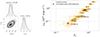 |
Fig. A.1. Example of fitting resultsLeft: Corner plot of posterior distributions for the two power-law parameters that describe the relationship between the peak energy and isotropic luminosity. Right: Data-resolved spectroscopy of the Fermi/GBM data for GRB 200415A (black) and the posterior predictive distribution (orange). To compute the posterior predictive distribution, we simulated the data generation process by first picking a set of parameters ( |
Appendix B: Time-resolved spectral analyses using fixed-time intervals
Time-resolved analyses: Fixed intervals.
Appendix C: Time-resolved analyses of GRB 200415A and GRB 180128A
Time-resolved spectral analysis using BBs.
Appendix D: Fit statistics
Best-fit model fits for GRB 231115A.
Appendix E: Optical and infrared follow-up observations
Optical and infrared observations of GRB 231115A.
Appendix F: Time-resolved spectral fits
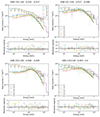 |
Fig. F.1. Time-resolved fits to a COMPT model using the BB time intervals. |
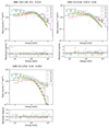 |
Fig. F.1. continued. |
All Tables
All Figures
|
Fig. 1. Fermi/GBM light curve of GRB 231115A (black), binned at a temporal resolution of counts per 3 ms, with the background model (green). The brown line is the result of the BB analysis of the burst. The pink dots are the time-resolved peak energy values taken from Table 1. At this finer temporal resolution we see a double-peaked structure within the initial burst signal. |
| In the text | |
|
Fig. 2. Time-integrated spectral fit to a COMPT model for GRB 231115A. |
| In the text | |
|
Fig. 3. Confidence contours for the time-resolved spectral analysis of GRB 231115A, corresponding to the BB intervals in Table 1. The contours represent the 50% and 90% confidence regions for the correlated parameters. Highlighted intervals illustrate spectral evolution within the burst. |
| In the text | |
|
Fig. 4. Energetic photons from GRB 231115A. Individual TTEs of GBM BGO detector 1 are indicated with black dots. The blue rectangle highlights energies from 655 keV to 930 keV, and the red rectangle energies from 930 keV to 1192 keV. We conclude that the highest photon energy associated with GRB 231115A is ∼900 keV. |
| In the text | |
|
Fig. 5. Luminosity distribution of M82 Chandra point sources within the INTEGRAL uncertainty region of GRB 231115A (light gray histogram). They are detected in the full Chandra exposure of the galaxy, totaling ≈1 Ms. The dark gray histogram represents the luminosity distribution of known magnetars. |
| In the text | |
|
Fig. 6. Detectability of short bursts with XMM-Newton (black and gray lines) and NuSTAR (blue and cyan lines), if the putative magnetar is coincident with the center of the galaxy or offset by a few arcminutes, respectively. The vertical dotted lines correspond to burst energy for which a trial-corrected confidence level is 99% for each case. See the main text for more details. |
| In the text | |
|
Fig. 7. Re-pointing simulation results. Left: Simulated MGF tail light curve with XRT (blue) and NICER (red) assuming the properties as observed in the SGR 1806−20 MGF tail, and scaling it to the M82 distance of 3.5 Mpc. The inset shows the modulation that is embedded in the light curve. Right: Z22 power for pulsation detection in XRT and NICER as a function of MGF distance. The dot-dashed and the dotted lines show the 4.5σ and 3σ detection significance (single-trial), respectively. The vertical dashed line is the M82 distance of 3.5 Mpc. See the main text for more details. |
| In the text | |
|
Fig. 8. Spectra of GRB 231115A over four BB time intervals. The intervals show the onset of the burst (1), peak 1 (2), peak 2 (4), and the extended emission after the peaks (5). Intervals (3), (6), and (7) are omitted for clarity but are consistent with the trend displayed. The shaded area indicates the 90% confidence regions. |
| In the text | |
|
Fig. 9. Comptonized spectrum peak energy (Ep) as a function of time using a temporal binning of 8 ms and values from Table B.1. All fit errors and error bars are at the 90% confidence level. The zero-time reflects the GBM event start time of each detection. |
| In the text | |
|
Fig. 10. Liso–Ep relation using different timing intervals. Left: Correlation between Liso and Ep for the four MGF candidates, GRB 231115A (light blue), GRB 051103 (pink), GRB 200415A (black), and GRB 180128A (gray), revealing an approximate |
| In the text | |
|
Fig. A.1. Example of fitting resultsLeft: Corner plot of posterior distributions for the two power-law parameters that describe the relationship between the peak energy and isotropic luminosity. Right: Data-resolved spectroscopy of the Fermi/GBM data for GRB 200415A (black) and the posterior predictive distribution (orange). To compute the posterior predictive distribution, we simulated the data generation process by first picking a set of parameters ( |
| In the text | |
|
Fig. F.1. Time-resolved fits to a COMPT model using the BB time intervals. |
| In the text | |
|
Fig. F.1. continued. |
| In the text | |
Current usage metrics show cumulative count of Article Views (full-text article views including HTML views, PDF and ePub downloads, according to the available data) and Abstracts Views on Vision4Press platform.
Data correspond to usage on the plateform after 2015. The current usage metrics is available 48-96 hours after online publication and is updated daily on week days.
Initial download of the metrics may take a while.