© The Authors 2024

1. Introduction

A magnetar is a type of young neutron star (NS) with an extremely strong magnetic field, which can reach strengths of ∼10¹⁵ G (e.g., Mereghetti 2008; Kaspi & Beloborodov 2017, for a review). The decay of the strong magnetic field can power strong emission, which is typically at X-ray and soft γ-ray bands with a duration from a few milliseconds to several months. The concept of the magnetar was first postulated for the pulsating gamma-ray burst (GRB) observed on March 9, 1979, in the Large Magellanic Cloud (LMC) (e.g., Mazets et al. 1979; Daugherty & Harding 1983; Usov 1984; Dermer 1990). With more observations including a regular 8 s oscillating decay and its localization (Cline et al. 1980, 1982), this event was later considered as a soft gamma repeater (SGR) rather than a typical GRB. Additionally, magnetars were then unified with anomalous X-ray pulsars (AXPs) by Thompson and Duncan (Thompson & Duncan 1993, 1996). Observations have revealed many similarities between AXPs and SGRs (Mereghetti 2008). Currently, there are nearly 30 candidate magnetars discovered in the Milky Way, as summarized in Kaspi & Beloborodov (2017).

Evidence for the existence of younger magnetars has been found in recent years (e.g., Kaspi & Beloborodov 2017). A very young radio-loud magnetar, Swift J1818.0−1607, was discovered in 2020 (Esposito et al. 2020). It has a spin period of 1.36 s and a characteristic age of 240 yr, and is presently the youngest known magnetar in the Milky Way. Hu et al. (2020) further revised the age of Swift J1818.0−1607 to ∼470 yr based on the observation by the Neutron star Interior Composition Explorer (NICER) team. Some high-energy outbursts from extragalactic magnetars have recently been observed. Several GRB-like events have been proposed to be actually magnetar giant flares (MGFs) after estimating their distances. MGFs are characterized by a typical duration of ∼0.1 s and an isotropic energy of ∼10⁴⁵ − 10⁴⁶ erg at the hard X-ray and soft γ-ray bands (e.g., Burns et al. 2021). For example, GRB 200415A is considered to be an extragalactic MGF with an isotropic energy of ≃1.36 × 10⁴⁶ erg and a distance of ≃3.5 Mpc (e.g., Minaev & Pozanenko 2020; Yang et al. 2020; Roberts et al. 2021; Svinkin et al. 2021). Zhang et al. (2022) proposed that the age of this magnetar is constrained to only a few weeks by interpreting the period in the decaying light curves as the rotation period. Recently, GRB 231115A, detected by INTEGRAL in M 82, has also been considered to be another possible extragalactic MGF (Wang et al. 2024; Mereghetti et al. 2024). In addition, extremely young magnetars have been suggested to be the central engines of GRBs and supernovae. The prolonged plateaus in the X-ray afterglows of some GRBs have been suggested to be mainly contributed by the energy injection from extremely young magnetars (e.g., Kouveliotou et al. 1998; Stratta et al. 2018). A similar mechanism involving extremely young magnetars can also explain the light curves of supernovae, in which the radiation from the radioactive decay of Ni is not enough to provide the observed luminosity (e.g., Kasen & Bildsten 2010).

Magnetars have also been confirmed as the central engines of at least some of the recorded fast radio bursts (FRBs). In 2020, a Galactic FRB 200428 with an isotropic energy of ∼10³⁵ erg (Pavlović et al. 2013; Zhong et al. 2020; Zhou et al. 2020; Yang & Zhang 2021) detected by CHIME (CHIME/FRB Collaboration 2020) and STARE2 (Bochenek et al. 2020) was confirmed as being related to the magnetar SGR 1935+2154, which has a characteristic age of about 3.6 kyr (Israel et al. 2016). This indicates that magnetars are at least one of the physical origins of FRBs. In addition, FRB 200428 was found to be associated with a magnetar short burst (MSB) of ∼0.5 s in duration and ∼10⁴⁰ erg in isotropic energy (Tavani et al. 2021), which shows magnetars can produce both MSBs and FRB-like radio bursts simultaneously. SGR 1935+2154 is regarded as one of the most burst-active SGRs (H.E.S.S. Collaboration 2022), emitting 127 bursts from 2014 to 2016 (Lin et al. 2020). In late April and May 2020, SGR 1935+2154 re-entered an active phase, and more than 217 bursts were detected (Younes et al. 2020). Many more bursts have been observed from this source since then, including a large episode in October, 2022 (Younes et al. 2022; Maan et al. 2022; Palmer & Swift/BAT Team 2022).

Additionally, young magnetars with a strong magnetic field and a fast rotation spin can produce an ultrarelativistic e⁺e⁻-pair wind (e.g., Rees & Gunn 1974; Kennel & Coroniti 1984a; Coroniti 1990; Kirk & Skjæraasen 2003), which could produce various observable features. Some studies have predicted radiation associated with such a pair wind. For example, Dai (2004) and Geng et al. (2016) studied the afterglow emission generated by the interaction of such a wind with a fireball from the GRB. If the magnetar is in a binary system, the radiation can be generated by the bow shock from the interaction between a magnetar e⁺e⁻-pair wind and a stellar wind (e.g., Cantó et al. 1996; Wilkin 1996; Bucciantini et al. 2005; Wadiasingh et al. 2017). In addition to the ultrarelativistic pair wind, Yang (2021) proposed that FRBs from a magnetar can heat the companion in a binary system and produce the re-emission at the optical band with a duration of a few hundred seconds. Some previous works have also studied the interaction process between the ejecta and the companion if a catastrophic event occurs in a binary system. The companion star can also have a shielding effect on the radiation from the burst (Zou et al. 2021), and MacFadyen et al. (2005) studied the X-ray flares generated by the interaction between the GRB outflow and a stellar companion with a relatively small distance. Furthermore, the radiation from the interaction of supernova ejecta and a companion star has also been studied (e.g., Kasen 2010).

It is common for stars to be in binary or even multiple star systems (e.g., Duchêne & Kraus 2013; Badenes et al. 2018). There have been several studies addressing the possibility of magnetars existing in binary systems (Chrimes et al. 2022; Bozzo et al. 2022; Xu et al. 2022). According to the simulation of Xu et al. (2022), there are probably magnetars in high-mass X-ray binaries. Observationally, Bozzo et al. (2022) proposed that the X-ray binary 3A 1954+319 is likely a system with a magnetar and an M supergiant. Also, Beniamini et al. (2023) studied a list of magnetar candidates in binaries. For the binary evolution process, several authors have studied the effects of supernova ejecta on binary star systems, and these studies found that the binary system can remain bound (Hirai et al. 2018). Observationally, Chen et al. (2024) reported a 12.4 day periodicity in SN 2022jli, which indicates the orbital period of a close binary system after a supernova. In addition to the classical binary evolution process, the formation of binary systems also includes the dynamic capture process. Lee et al. (2010) proposed that the binary system including compact objects can also be generated by the dynamic capture in dense stellar environments. In this way, the prior activity from the magnetar, including the supernova ejecta, will not destroy the binary system.

In this theoretical work, we consider a magnetar in a close binary system with a main sequence star as the companion. Once a burst (e.g., FRBs, MSBs, and MGFs) occurs on a magnetar, it will interact with a companion star due to its high radiation pressure. Here we mainly analyze three types of bursts: FRBs, MSBs, and MGFs. The blackbody radiation can be generated via bursts heating the companion star due to the optically thick companion surface. The ultrarelativistic e⁺e⁻-pair wind from the magnetar interacts with the companion star or its stellar wind and generates sustained radiation that we refer to as the persistent preburst radiation. Bhardwaj et al. (2021) reported a repeating FRB 20200120E associated with a globular cluster with an age of ∼9.13 Gyr in M 81, which is a spiral galaxy at 3.63 ± 0.34 Mpc, where the number of main sequence and NSs could be as large as ≳10² (Kremer et al. 2021). Therefore, it is natural to consider the possibility of electromagnetic radiation being produced by a binary system with a magnetar, as analyzed by Yang (2021) for the case of FRBs, and it is crucial that we improve our understanding of the observed features of FRBs and/or other various bursts (e.g., MSB and MGF) and their progenitors, considering the scarcity of confirmed observations of electromagnetic signals associated with FRBs.

We calculate the persistent preburst radiation produced by the magnetar wind, and the re-emission from bursts interacting with the companion in Sects. 2.1 and 2.2. We then calculate the spectra and the light curves for such radiation and consider its detectability with optical (the Vera C. Rubin Observatory) and X-ray telescopes (Einstein Probe, Chandra and XMM-Newton) in Sect. 3.1. Finally, in Sect. 3.2, we scan the parameter space to determine whether the radiation from the magnetar wind and/or the magnetar bursts might be obscured by the radiation from the companion star, and find the parameter space in which the re-emission from bursts dominates.

We use the notation Q_x = Q/10^x in CGS units, except t_yr ≡ t/1 yr, M_{c, 1 M⊙} = M_c/1 M_⊙, R_{c, 1 R⊙} = R_c/1 R_⊙, and L_{c, 1 L⊙} = L_c/1 L_⊙.

2. Model

In this section, we discuss the physical processes of (1) the persistent preburst radiation from the interaction between the ultrarelativistic e⁺e⁻-pair wind from the magnetar and the companion or its stellar wind; and (2) the re-emission from the interaction between the magnetar bursts and the companion, which appears to be transient relative to the persistent preburst radiation, as shown in Fig. 1. In this case, the persistent preburst radiation is considered as the background before and after the generation of the re-emission from bursts, as shown in the bottom panel of Fig. 1. A magnetar is in a binary system with a main sequence star with M_c ∼ 0.1 − 20 M_⊙. This radiation could be observable as long as the line of sight is not obstructed by the companion.

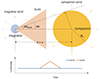Fig. 1. Schematic picture of radiation generated by a burst and/or a wind from a magnetar interacting with a main sequence star in a binary system. The persistent preburst radiation is generated by a strong magnetar wind heating a companion star, or by the bow shock from a weak magnetar wind interacting with a stellar wind from a companion star. The radiation from the transient is generated by the re-emission process from the companion star heated by a magnetar burst (e.g., an FRB, an MSB, and/or an MGF).

2.1. Persistent preburst radiation

The persistent preburst radiation can be divided into two cases based on the luminosity of the magnetar wind L_w, as shown in Fig. 2. We refer to the scenario where the magnetar wind directly interacts with the companion star as Case I, while we refer to the scenario in which the magnetar wind interacts with the companion wind to produce a bow shock as Case II.

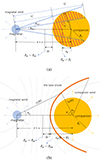Fig. 2. Schematic picture of the persistent preburst radiation. In the top panel, we show the scenario (Case I) where the magnetar wind directly interacts with the companion star. In the bottom panel, we indicate the scenario (Case II) where the bow shock is generated by the interaction between the magnetar wind and the possible strong companion wind.

For a strong magnetar wind, it will directly interact with the companion star, as shown in Fig. 2a. In this process, the bow shock will not be generated, because the pressure of the magnetar wind will be so high that the pressure equilibrium position of the two winds (i.e., the magnetar wind and the companion wind) will be inside the companion star. The magnetar wind will penetrate the companion and stop at r_b, where the pressure of the magnetar wind P_w is equal to the internal pressure P_c of the companion star. The energy from the magnetar wind will then be transferred to the swept medium of the companion star. We approximate that the pressure of the magnetar wind inside the companion star is a constant, because d ≫ R_c, where d is the distance between the magnetar and the companion star, and R_c is the radius of the companion star. Therefore, the heated region of the companion is the shaded orange area in Fig. 2a, and the re-emission can then be generated considering the black-body radiation.

For a relatively weak magnetar wind, the bow shock will be generated by the interaction between the magnetar wind and the companion wind at r_b, where the momentum conservation is satisfied. In Fig. 2b, the dashed gray line shows the geometry of the bow shock with different L_w. The main radiation is contributed by the shock head considering the synchrotron process, and we assume the radiation region is a cone surface with a width of Δ_bow.

2.1.1. Criteria for distinguishing Case I from Case II

In this section, we provide a detailed explanation of how to differentiate between Case I and Case II. For an extremely young magnetar with a millisecond spin period, the luminosity of a highly relativistic wind dominated by the energy flux of e⁺e⁻ pairs is

$$\begin{array}{c}\hfill L_{\mathrm{w}}=L_{\mathrm{w},0}{(1+\frac{T_{\mathrm{age}}}{T_{\mathrm{sd}}})}^{-2},\end{array}$$(1)

where $L_{\mathrm{w},0}\simeq 9.6\times {10}^{44}\mathrm{erg}{\mathrm{s}}^{-1}{B}_{\perp ,15}^2{R}_{\mathrm{M},6}^6{P}_{0,-2}^{-4}$ is the initial spin-down luminosity, $T_{\mathrm{sd}}\simeq 2.3\times {10}^5\mathrm{s}{B}_{\perp ,15}^{-2}{I}_{45}{R}_{\mathrm{M},6}^{-6}{P}_{0,-2}^2$ is the initial spin-down timescale of the magnetar, B_⊥ is the surface dipolar magnetic field of the magnetar, $I=2/5\left(M_{\text{m}}{R}_{\text{m}}^2\right)$ is the moment of inertia of the magnetar, R_m is the radius of the magnetar, M_m is the mass of the magnetar, and T_age is the age of the magnetar. P₀ is the initial rotation period of the magnetar. The theoretical value of P₀ can be as low as ∼0.3 − 0.5 ms (Cook et al. 1994; Koranda et al. 1997). We note that the observed rotation period of the Galactic magnetar ranges from 0.32 to 12 s (Archibald et al. 2015; Kaspi & Beloborodov 2017; Kuiper et al. 2018), and this is because of the magnetar spindown, which dictates that most Galactic magnetars with ages of a few hundred years to tens of thousands of years will have relatively long periods. To be consistent with the observed persistent X-ray luminosity for Galactic magnetars (Olausen & Kaspi 2014), here we use P₀ = 10⁻² s, B_⊥ = 10¹⁵ G, M_m = 1.4 M_⊙, and R_m = 10⁶ cm unless stating otherwise.

The pressure of the relativistic wind should be

$$\begin{array}{c}\hfill P_{\mathrm{w}}\simeq \frac{1}{3}{U}_{\mathrm{w}}=\frac{L_{\mathrm{w}}}{12\pi {(d-r)}^{2}c},\end{array}$$(2)

where r is the distance between the area we study and the companion, as shown in Fig. 2. We use the semimajor axis a of the binary system to approximate d (which applies to binary systems with a relatively small eccentricity), that is

$$\begin{array}{c}\hfill a={\left(\frac{G{M}_{\mathrm{tot}}{P}_{\mathrm{orb}}^2}{4{\pi }^2}\right)}^{1/3},\end{array}$$(3)

where M_tot = M_c + M_m is the total mass of the binary system, M_c is the mass of the companion, and P_orb is the orbital period of the binary system.

The pressure of the companion wind is

$$\begin{array}{c}\hfill P_{\mathrm{cw}}={\rho }_{\mathrm{cw}}{v}_{\mathrm{cw}}^2=\frac{\dot{M}{v}_{\mathrm{cw}}}{4\pi r^2},\end{array}$$(4)

where Ṁ is the mass-loss rate, which depends on the companion type, and v_cw is the velocity of the companion wind. Based on Vink et al. (2000), we estimate the mass-loss rate for O stars, B stars, and solar-like stars:

$$\begin{array}{c}\hfill \log \dot{M}\simeq \{\begin{array}{cc}& -12.21,T_{\mathrm{c},\mathrm{eff}}\le 12500\mathrm{K},\hfill \\ \hfill & -6.688+2.210\log \left(\frac{L_{\mathrm{c}}}{{10}^5{L}_{\odot }}\right)\hfill \\ \hfill & -1.339\log \left(\frac{M_{\mathrm{c}}}{30M_{\odot }}\right)-1.601\log \left(\frac{v_{\mathrm{esc}}}{v_{\mathrm{cw},\infty }}\right)\hfill \\ \hfill & +1.07\log \left(\frac{T_{\mathrm{c},\mathrm{eff}}}{2\times {10}^4\mathrm{K}}\right),\hfill \\ \hfill & 12500\mathrm{K}<T_{\mathrm{c},\mathrm{eff}}\le 22500\mathrm{K},\hfill \\ \hfill & -6.697+2.194\log \left(\frac{L_{\mathrm{c}}}{{10}^5{L}_{\odot }}\right)-1.313\log \left(\frac{M_{\mathrm{c}}}{30M_{\odot }}\right)\hfill \\ \hfill & -1.226\log \left(\frac{v_{\mathrm{esc}}}{v_{\mathrm{cw},\infty }}\right)+0.933\log \left(\frac{T_{\mathrm{c},\mathrm{eff}}}{4\times {10}^4\mathrm{K}}\right)\hfill \\ \hfill & -10.92{\left[\log \left(\frac{T_{\mathrm{c},\mathrm{eff}}}{4\times {10}^4\mathrm{K}}\right)\right]}^2,\hfill \\ \hfill & 22500\mathrm{K}<T_{\mathrm{c},\mathrm{eff}}\le 100000\mathrm{K},\hfill \end{array}\end{array}$$(5)

where Ṁ is in M_⊙ yr⁻¹, L_c is the luminosity of the companion, v_cw, ∞ is the velocity of the stellar wind at an infinite distance from the companion, v_esc = (2GM_c/R_c)^1/2 is the escaping velocity from the companion star, and T_c,eff is the effective temperature of the companion. We note that for solar-like stars, we set Ṁ ≃ 6.17 × 10⁻¹³ M_⊙ yr⁻¹, which is consistent with the range mentioned in Wood et al. (2002). We use the following mass–luminosity relation and mass–radius relation to calculate L_c and R_c from M_c (Iben 2012; Salaris & Cassisi 2005):

$$\begin{array}{c}\hfill L_{\mathrm{c},1L_{\odot }}\simeq \{\begin{array}{cc}0.23M_{\mathrm{c},1M_{\odot }}^{2.3}\hfill & M_{\mathrm{c}}\le 0.43M_{\odot }\hfill \\ M_{\mathrm{c},1M_{\odot }}^4\hfill & 0.43M_{\odot }<M_{\mathrm{c}}\le 2M_{\odot }\hfill \\ 1.4M_{\mathrm{c},1M_{\odot }}^{3.5}\hfill & 2M_{\odot }<M_{\mathrm{c}}\le 55M_{\odot }\hfill \\ 32000M_{\mathrm{c},1M_{\odot }}\hfill & 55M_{\odot }<M_{\mathrm{c}}\hfill \end{array},\end{array}$$(6)

$$\begin{array}{c}\hfill R_{\mathrm{c},1R_{\odot }}\simeq \{\begin{array}{cc}{M}_{\mathrm{c},1M_{\odot }}^{0.8}\hfill & M_{\mathrm{c}}\le 1M_{\odot }\hfill \\ M_{\mathrm{c},1M_{\odot }}^{0.57}\hfill & 1M_{\odot }<M_{\mathrm{c}}\hfill \end{array}.\end{array}$$(7)

Furthermore, we obtain the effective temperature T_c,eff using $4\pi R_{\text{c}}^2\sigma T_{\text{c},\text{eff}}^4=L_{\text{c}}$. In real observations, the effective temperature T_c, eff can be measured via the spectrum of the companion star assuming that it satisfies the black-body radiation.

Based on Vink et al. (2000), we use v_esc/v_cw, ∞ = 0.7 for a solar-like star, v_esc/v_cw, ∞ = 1.3 for a B star, and v_esc/v_cw, ∞ = 2.6 for an O star. We can then obtain Ṁ at a given M_c. In addition, the velocity of the stellar wind v_cw at r is

$$\begin{array}{c}\hfill v_{\mathrm{cw}}=v_{\mathrm{cw},\infty }{(1-\frac{R_{\mathrm{c}}}{r})}^{1/2}.\end{array}$$(8)

We approximate that v_cw ≈ v_cw, ∞ when r ≳ R_c. We derive the pressure of the companion wind P_cw at a given M_c and a given r using Eqs. (4)–(8).

Assuming P_w = P_cw and combining with Eqs. (1)–(8), we can derive the location of the bow shock r_b at the line connecting the two stars by numerically solving the following equation:

$$\begin{array}{c}\hfill \frac{r_{\mathrm{b}}^4}{{(d-r_{\mathrm{b}})}^4}={\beta }_{\mathrm{b}}^2(1-\frac{R_{\mathrm{c}}}{r_{\mathrm{b}}}),\end{array}$$(9)

where β_b = L_w/(3Ṁv_cw,∞c) is the ratio of the pressure for the magnetar wind and the companion wind. When r_b ≳ R_c, we can obtain the following approximate equation:

$$\begin{array}{c}\hfill r_{\mathrm{b}}\approx \frac{1}{1+\sqrt{{\beta }_{\mathrm{b}}}}a.\end{array}$$(10)

According to Eqs. (4) and (8), we know that P_cw ≤ P_cw, ∞, where P_cw, ∞ is the pressure of the companion wind with v_cw = v_cw, ∞. Therefore, we use Eq. (10) to approximately determine Case I and Case II. Only when r_b is larger than R_c (corresponding to the lower limit of T_age) and d − r_b is larger than R_LC (corresponding to the upper limit of T_age) can a bow shock be generated between a magnetar and a companion star, where R_LC = P_mc/(2π) is the light cylinder of the magnetar and P_m = P₀(1+T_age/T_sd)^1/2 is the rotation period of the magnetar. We can then get the limitation of L_w and T_age for a given P_orb and M_c at which the bow shock would exist, as shown in the colored region in Fig. 3. We find that the larger the value of P_orb, the larger the upper limit on L_w and the smaller the lower limit on T_age for the bow shock. We also find that for P_orb = 10 d, the generation of the bow shock requires 2.6 × 10³⁰ erg s⁻¹ ≲ L_w ≲ 9.6 × 10³⁴ erg s⁻¹ (4.8 × 10³² erg s⁻¹ ≲ L_w ≲ 1.6 × 10³⁸ erg s⁻¹) with M_c = 1 M_⊙ (M_c = 10 M_⊙); and for P_orb = 100 d, it requires 3.0 × 10²⁹ erg s⁻¹ ≲ L_w ≲ 2.2 × 10³⁶ erg s⁻¹ (6.1 × 10³¹ erg s⁻¹ ≲ L_w ≲ 4.0 × 10³⁹ erg s⁻¹) with M_c = 1 M_⊙ (M_c = 10 M_⊙). In this way, we can divide our calculation for the persistent preburst radiation into two cases, Case I and Case II, as described above. We note that here we focus on Case I and Case II, and neglect the condition d − r_b < R_LC, in which the companion wind directly interacts with the magnetar.

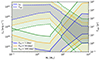Fig. 3. Permitted luminosity of the magnetar wind and the corresponding age of the magnetar for a given Mc which varies from 0.1 M⊙ to 100 M⊙, at which the magnetar wind will interact with the companion wind with the generation of the bow shock. Different colors represent different values of Porb, as indicated in the caption. The solid lines show the luminosity of the magnetar wind, while the dashed lines indicate the age of the magnetar. The colored areas show the permitted parameter for the scenario where the bow shock is generated from the interaction between the magnetar wind and the companion wind.

2.1.2. Effects of magnetar winds on companion stars

Now, we consider whether a magnetar has enough energy to evaporate its main sequence companion in a binary system (also see Bhattacharya & van den Heuvel 1991). The energy reservoirs of a magnetar include the rotation energy,

$$\begin{array}{c}\hfill E_{\mathrm{rot}}=\frac{1}{2}I{\mathrm{\Omega }}_{\mathrm{rot}}^2,\end{array}$$(11)

and the magnetic energy,

$$\begin{array}{c}\hfill E_{\mathrm{B}}\lesssim \frac{1}{6}{B}_{\perp }^2{R}_{\mathrm{m}}^3,\end{array}$$(12)

where P = 2π/Ω is the spin period of the magnetar, B_⊥ is the perpendicular component of the surface dipolar magnetic field of the magnetar, and R_m is the radius of the magnetar. We define the efficiency g = f(R_c/2a)² as the fraction of the magnetar’s rotation energy and/or magnetic energy that actually contributes to the evaporation of the companion, where (R_c/2a)² is the geometric factor, and f refers to the “real” efficiency of the evaporation process (Bhattacharya & van den Heuvel 1991). The gravitational binding energy of the companion is

$$\begin{array}{c}\hfill E_{\mathrm{b}}\simeq \frac{G{M}_{\mathrm{c}}^2}{R_{\mathrm{c}}}.\end{array}$$(13)

The condition under which the magnetar can completely evaporate its companion is

$$\begin{array}{c}\hfill \frac{gmax(E_{\mathrm{rot}},E_{\mathrm{B}})}{E_{\mathrm{b}}}\ge 1.\end{array}$$(14)

For the following typical magnetar values, that is, P₀ = 10⁻² s, B_⊥ = 10¹⁵ G, M_m = 1.4 M_⊙, and R_m = 10⁶ cm, a companion with a mass of M_c = 0.1 − 20 M_⊙ in a binary system with an orbital period of P_orb = 1 − 1000 d cannot be completely evaporated by a magnetar even with f = 1.

We now consider the effects of partial evaporation on our model. The evaporation timescale of the companion τ_evap can be estimated as

$$\begin{array}{c}\hfill {\tau }_{\mathrm{evap}}\simeq \frac{g_{\mathrm{par}}{E}_{\mathrm{b}}}{g{L}_{\mathrm{w},0}},\end{array}$$(15)

where g_par ∼ m_evap/M_c indicates the fraction of partial evaporation compared to complete evaporation, and m_evap is the mass of the outer layers of the companion that may be evaporated. If the value of τ_evap is larger than the spin-down timescale of the magnetar T_sd, the companion can survive and keep its structure, since the luminosity of the magnetar wind will drop sharply after T_sd. For the typical values we choose for a magnetar, the evaporation timescale of a companion with M_c = 0.1 − 20 M_⊙ and P_orb = 1 − 1000 d is 5.1 × 10⁵ s − 2.8 × 10¹⁰ s with g_par ≳ 0.01 and f = 0.01 (Bhattacharya & van den Heuvel 1991), which is larger than T_sd ≈ 2.3 × 10⁵ s. For a smaller value of g_par (≲0.01), we consider the hydrostatic equilibrium timescale of the companion, which is ${\tau }_{\mathrm{hyd}}\simeq 3\times {10}^3\mathrm{s}\sqrt{{\overline{\rho }}_{\mathrm{c}}/{\overline{\rho }}_{\odot }}$ (where ${\overline{\rho }}_{\odot }=1.4\mathrm{g}{\mathrm{cm}}^{-3}$ is the average density of the Sun, and ${\overline{\rho }}_{\mathrm{c}}=3M_{\mathrm{c}}/\left(4\pi R_{\mathrm{c}}^3\right)$ is the average density of the companion). This timescale refers to the time it takes for the companion to become spherical again after its spherical shape is destroyed. We can see that the value of τ_hyd ≃ 1.3 × 10³ s − 1.5 × 10⁴ s is much smaller than P_orb and τ_evap (unless the value of g_par is extremely small, where the evaporation process can be neglected), meaning that the companion can remain spherical in our model even if a small part of it is evaporated with g_par ≲ 0.01.

Therefore, we believe that, at least within the confines of the model we study, the companion star can remain spherical and its evaporation process can be neglected. Below, for simplicity, we use the Lane-Emden model with n = 3 to simulate the internal structure of the companion star. This model is associated with a fully radiative star, where it is assumed that the ratio between the gas pressure and the total pressure is a constant throughout the star, which fits well with the internal structure of the Sun (Guenther et al. 1992) and very massive stars (Nadyozhin & Razinkova 2005). The Lane-Emden equation is

$$\begin{array}{c}\hfill \frac{1}{{\xi }^2}\frac{\mathrm{d}}{\mathrm{d}\xi }\left({\xi }^2\frac{\mathrm{d}{\theta }_{\mathrm{LE}}}{\mathrm{d}\xi }\right)=-{\theta }_{\mathrm{LE}}^n,\end{array}$$(16)

where θ_LE and ξ = r/r_n is the dimensionless parameter, $r_n={[(n+1)K{\rho }_{\mathrm{ce}}^{1/n-1}/(4\pi G)]}^{1/2}$ is a typical radius, K is a constant, and ${\rho }_{\mathrm{ce}}=M_{\mathrm{c}}/\left[4\pi R_{\mathrm{c}}^3{(-\frac{1}{\xi }\frac{\mathrm{d}{\theta }_{\mathrm{LE}}}{\mathrm{d}\xi })}_{\xi ={\xi }_1}\right]$ is the density at the center of the companion star. We note that ξ₁ = R_c/r_n indicates the surface of the companion star, where θ_LE(ξ₁) = 0. The internal density of the companion is ${\rho }_{\text{c}}={\rho }_{\text{ce}}{\theta }_{\text{LE}}^n$, and the internal pressure of the companion is $P_{\mathrm{c}}=K{\rho }_{\mathrm{c}}^{1+\frac{1}{n}}$. Numerically solving Eq. (16), we can obtain the internal structure of the companion for a given M_c, including P_c and ρ_c at each radius r = ξr_n.

2.1.3. Radiation from the direct interaction between magnetar wind and companion star

In Case I, the luminosity of the magnetar wind is sufficiently high that it will directly interact with the companion star and heat it. Following Yang (2021), who analyzed the process by which an FRB heats the companion surface, we consider that the magnetar wind terminates at r_b. The value of r_b is determined by numerically solving the equation P_w(r) = P_c(r) using Eqs. (2) and (16). The thickness of the shocked medium at θ_m = 0 is l = R_c − r_b. We note that for M_c = 0.1 − 20 M_⊙ and P_orb = 1 − 1000 d, the value of l/R_c is smaller than 0.1, meaning that the spherical shape of the companion star is not significantly affected, and we can still use the Lane-Emden equation to approximate the structure of the companion.

We construct a spherical coordinate system with the center of the magnetar as the origin and the vector from the magnetar to the companion star as the z-axis. We divide the heating region into two parts, θ_m ∈ (0, θ_m1) (region I) and θ_m ∈ (θ_m1, θ_m2) (region II), where ${\theta }_{\mathrm{m}1}=arcsin\frac{r_{\mathrm{b}}}{a}$ and ${\theta }_{\mathrm{m}2}=arcsin\frac{R_{\mathrm{c}}}{a}$, as shown in Fig. 2a. The volume of the heating region of the companion star is

$$\begin{array}{cc}\hfill V_{\mathrm{sw}}& =2\pi {\displaystyle {\int }_0^{{\theta }_{\mathrm{m}1}}}{\displaystyle {\int }_{r{\prime }_{x_1}}^{r{\prime }_{y_1}}}r{\prime }^{2}sin{\theta }_{\mathrm{m}}\mathrm{d}r\prime \mathrm{d}{\theta }_{\mathrm{m}}\hfill \\ \hfill & +2\pi {\displaystyle {\int }_{{\theta }_{\mathrm{m}1}}^{{\theta }_{\mathrm{m}2}}}{\displaystyle {\int }_{r{\prime }_{x_2}}^{r{\prime }_{y_2}}}r{\prime }^{2}sin{\theta }_{\mathrm{m}}\mathrm{d}r\prime \mathrm{d}{\theta }_{\mathrm{m}},\hfill \end{array}$$(17)

where $r{\prime }_{x_1}=r{\prime }_{x_2}=acos{\theta }_{\mathrm{m}}-\sqrt{a^2({cos}^2{\theta }_{\mathrm{m}}-1)+R_{\mathrm{c}}^2}$ and $r{\prime }_{{\mathit{y}}_1}=acos{\theta }_{\mathrm{m}}-\sqrt{a^2({cos}^2{\theta }_{\mathrm{m}}-1)+r_{\mathrm{b}}^2}$ are the boundary of region I, and $r_{x_1}^{\prime }=r_{x_2}^{\prime }$ and $r{\prime }_{{\mathit{y}}_2}=acos{\theta }_{\mathrm{m}}+\sqrt{a^2({cos}^2{\theta }_{\mathrm{m}}-1)+R_{\mathrm{c}}^2}$ are the boundary of region II. The mass of the heating region is

$$\begin{array}{cc}\hfill m_{\mathrm{sw}}& =2\pi {\displaystyle {\int }_0^{{\theta }_{\mathrm{m}1}}}{\displaystyle {\int }_{r{\prime }_{x_1}}^{r{\prime }_{y_1}}}{\rho }_{\mathrm{c}}r{\prime }^{2}sin{\theta }_{\mathrm{m}}\mathrm{d}r\prime \mathrm{d}{\theta }_{\mathrm{m}}\hfill \\ \hfill & +2\pi {\displaystyle {\int }_{{\theta }_{\mathrm{m}1}}^{{\theta }_{\mathrm{m}2}}}{\displaystyle {\int }_{r{\prime }_{x_2}}^{r{\prime }_{y_2}}}{\rho }_{\mathrm{c}}r{\prime }^{2}sin{\theta }_{\mathrm{m}}\mathrm{d}r\prime \mathrm{d}{\theta }_{\mathrm{m}}.\hfill \end{array}$$(18)

We note that the distance between the point in the heating region and the center of the companion is $r_l=\sqrt{r^{\prime 2}-2drcos{\theta }_{\mathrm{m}}+a^2}$, and we can then derive the density ρ_c = ρ_c(r_l) for a given r′. In this way, the mass of the heating region can be calculated. The injection energy is

$$\begin{array}{cc}\hfill \mathcal{E}& =2\pi {\displaystyle {\int }_0^{{\theta }_{\mathrm{m}1}}}{\displaystyle {\int }_{r{\prime }_{x_1}}^{r{\prime }_{y_1}}}\frac{L_{\mathrm{w}}}{4\pi r{\prime }^{2}c}r{\prime }^{2}sin{\theta }_{\mathrm{m}}\mathrm{d}r\mathrm{d}{\theta }_{\mathrm{m}}\hfill \\ \hfill & +2\pi {\displaystyle {\int }_{{\theta }_{\mathrm{m}1}}^{{\theta }_{\mathrm{m}2}}}{\displaystyle {\int }_{r{\prime }_{x_2}}^{r{\prime }_{y_2}}}\frac{L_{\mathrm{w}}}{4\pi r{\prime }^{2}c}r{\prime }^{2}sin{\theta }_{\mathrm{m}}\mathrm{d}r\prime \mathrm{d}{\theta }_{\mathrm{m}}\hfill \\ \hfill & =\frac{L_{\mathrm{w}}}{2c}{\displaystyle {\int }_0^{{\theta }_{\mathrm{m}1}}}{\displaystyle {\int }_{r{\prime }_{x_1}}^{r{\prime }_{y_1}}}sin{\theta }_{\mathrm{m}}\mathrm{d}r\mathrm{d}{\theta }_{\mathrm{m}}+\frac{L_{\mathrm{w}}}{2c}{\displaystyle {\int }_{{\theta }_{\mathrm{m}1}}^{{\theta }_{\mathrm{m}2}}}{\displaystyle {\int }_{r{\prime }_{x_2}}^{r{\prime }_{y_2}}}sin{\theta }_{\mathrm{m}}\mathrm{d}r\prime \mathrm{d}{\theta }_{\mathrm{m}}.\hfill \end{array}$$(19)

This energy will transfer to particles of the heating region. The number of these particles and the temperature of the heating region should be (Yang 2021)

$$\begin{array}{cc}& N=\frac{f_{\mathrm{b}}{m}_{\mathrm{sw}}}{m_{\mathrm{p}}},\hfill \\ \hfill & T=\frac{\eta \mathcal{E}}{\mathit{Nk}},\hfill \end{array}$$(20)

where η ∼ 0.01 − 0.1 is the factor accounting for energy losses during the energy transformation process, and f_b ∼ 0.1 − 1 is a corrected fraction for the mass of the companion swept by the magnetar wind since the above mass is an overestimated approximation. Here, we use η = 0.01 and f_b = 0.1 for an example.

Considering the radiative transfer process, the optical depth for the Thomson scattering at θ_m = 0 can be estimated as

$$\begin{array}{c}\hfill \tau \simeq {\displaystyle {\int }_0^l}\kappa {\rho }_{\mathrm{c}}(r_{\mathrm{b}}+l_{\mathrm{r}})\mathrm{d}{l}_{\mathrm{r}},\end{array}$$(21)

where κ ∼ 0.4 cm² g⁻¹ is the Thomson scattering opacity of fully ionized hydrogen, and ρ_c(r_b + l_r) is the internal density of the companion at r_b + l_r (l_r is from 0 to l). We use this optical depth to approximately calculate the effective temperature of the heating region based on the theory of radiative transfer (Yang 2021):

$$\begin{array}{c}\hfill T_{\mathrm{eff}}=T{(\frac{1}{2}+\frac{3}{4}\tau )}^{-1/4}.\end{array}$$(22)

Based on the above equations and the black-body radiation theory, the total luminosity of re-emission generated by the magnetar wind heating the companion can be estimated as

$$\begin{array}{c}\hfill L_{\mathrm{re}}\simeq 2\pi R_{\mathrm{c}}^2{\sigma }_{\mathrm{SB}}{T}_{\mathrm{eff}}^4,\end{array}$$(23)

where σ_SB is the Stefan-Boltzmann constant. The specific luminosity is

$$\begin{array}{c}\hfill L_{\nu }=2{\pi }^2{R}_{\mathrm{c}}^2\frac{2h{\nu }^3}{c^2}\frac{1}{e^{h\nu /(k{T}_{\mathrm{eff}})}-1}.\end{array}$$(24)

In addition, we compare the gravitational binding energy of the swept mass of the companion g_parE_b ≃ Gm_sw(M_c − m_sw)/r_b and the injection energy ηℰ. We find that in typical parameter spaces we choose, the value of ηℰ is much smaller than g_parE_b, and their ratio is ≲10⁻³. Therefore, we neglect the evaporation process of the companion caused by the magnetar wind in our work.

2.1.4. Radiation from the interaction between magnetar wind and companion wind

In Case II, the interaction between the magnetar wind and the companion wind generates a bow shock at r_b when L_w is small enough, as shown in Fig. 3. Following the analytical calculations in Wadiasingh et al. (2017) and Kong et al. (2011), we calculate the synchrotron radiation from the bow shock. We use the geometry of the bow shock proposed in Cantó et al. (1996). For more complex cases, a hydrodynamic simulation was performed to study this issue (Zabalza et al. 2013) and two-region models of two shocks have been studied (Usov 1992). It is noteworthy that the structure of the bow shock calculated by the analytical method is approximately consistent with that found using a numerical method (Zabalza et al. 2013). Also, many previous studies (e.g., Wadiasingh et al. 2017; Chen et al. 2019, 2021) that use similar methods to that presented here can model the observations of gamma-ray binaries and millisecond pulsar binaries very well. In this way, as part of our analysis, we use the above model to calculate the radiation. For β_b > 1, the magnetar wind is stronger, meaning that the bow shock bends toward the companion. The shape of the bow shock using the linear and angular momentum conservation is

$$\begin{array}{cc}& r_{\mathrm{b}}(\theta )=dsin{\theta }_{\mathrm{m}}csc(\theta +{\theta }_{\mathrm{m}}),\hfill \\ \hfill & r_{\mathrm{s}}(\theta )=dsin\theta csc(\theta +{\theta }_{\mathrm{m}}),\hfill \\ \hfill & {\theta }_{\mathrm{m}}cot{\theta }_{\mathrm{m}}=1+{\beta }_{\mathrm{b}}(\theta cot\theta -1),\hfill \end{array}$$(25)

where θ is the angle measured from the line between two stars with the companion as the origin, θ_m is the angle with the magnetar as the origin, and r_s is the distance between the bow shock and the magnetar, as shown in Fig. 2b. When θ = 0, the location of the bow shock can be derived using Eq. (10). The asymmetric angle θ_∞ of the bow shock wing, corresponding to r_b → ∞,  can be calculated using

$$\begin{array}{c}\hfill {\theta }_{\infty }-tan{\theta }_{\infty }=\frac{\pi }{1-{\beta }_{\mathrm{b}}}.\end{array}$$(26)

We estimate the volume of the radiation region to be

$$\begin{array}{c}\hfill V_{\mathrm{bow}}=2\pi {\mathrm{\Delta }}_{\mathrm{bow}}{\displaystyle {\int }_0^{{\theta }_{\infty }}}{\displaystyle {\int }_0^{r_{\mathrm{b}}(\theta )}}{r}^{2}sin\theta \mathrm{d}r\mathrm{d}\theta ,\end{array}$$(27)

where ${\mathrm{\Delta }}_{\mathrm{bow}}=\frac{1}{8}\min [r_{\mathrm{b}}(\theta =0),r_{\mathrm{s}}(\theta =0)]$ is the estimated thickness of the shocked shell (Luo et al. 1990). Conversely, for β_b < 1, the companion wind is stronger, and the bow shock bends toward the magnetar. For Eqs. (25)–(27), we need to replace r_b with r_s and θ_m with θ for β_b < 1. We estimate the equatorial upstream wind magnetic field to be (e.g., Kong et al. 2011)

$$\begin{array}{c}\hfill B_{\mathrm{w}}^2=\frac{\sigma L_{\mathrm{w}}}{r_{\mathrm{s}}^{2}c(1+\sigma )}.\end{array}$$(28)

We note that for different θ and/or θ_m, we have different values of B_w. Kennel & Coroniti (1984a,b) suggested that the pulsar wind magnetization σ, that is, the ratio of the magnetic energy flux to particle energy flux upstream of the shock, is ∼0.003 for the Crab pulsar wind nebula (PWN) based on observations, while Shibata et al. (2003) proposed a modified model considering magnetic-field turbulence, which gives σ ∼ 0.05. Here we use $\sigma =B_{\mathrm{w}}^2/(4\pi n_{\mathrm{e},\mathrm{w}}\langle {\gamma }_{\mathrm{w}}\rangle m_{\mathrm{e}}{c}^2)=0.01$ to obtain an estimation of the mean Lorentz factor of the radiation region ⟨γ_w⟩ (Wadiasingh et al. 2017; van der Merwe et al. 2020):

$$\begin{array}{c}\hfill \langle {\gamma }_{\mathrm{w}}\rangle \simeq {\left(\frac{L_{\mathrm{w}}}{c}\right)}^{1/2}\frac{5e}{{\mathcal{M}}_{\pm }{m}_{\mathrm{e}}{c}^2},\end{array}$$(29)

where e is the electron charge, $n_{e,w}\approx {\mathcal{M}}_{\pm }\sqrt{6c{L}_{\mathrm{w}}}/\left(4\pi ec{r}_{\mathrm{s}}^2\right)$ is the total number density of electrons in the radiation region contributed by the magnetar wind, and ℳ_± is the pair multiplicity of the Goldreich-Julian rate. The value of ℳ_± for a magnetar could be very different, because it highly depends on parameters (such as P and B_⊥) due to the photon splitting and pair creation (e.g., Thompson 2008; Chen & Beloborodov 2017). The theoretical estimation of multiplicity for the magnetar is ∼10² − 10⁴ (Medin & Lai 2010; Beloborodov 2013), while the young pulsar wind nebula and double pulsar studies (e.g., Sefako & de Jager 2003; Breton et al. 2012) suggest ℳ_± ∼ 10³ − 10⁵ (Wadiasingh et al. 2017). Here we use ℳ_± = 10⁴ as the typical value. Based on the shock jump condition for small σ in Kennel & Coroniti (1984b), the magnetic field of the shocked region is B_bow = 3(1 − 4σ)B_w ≃ 3B_w, and the Lorentz factor of the shocked region is ${\gamma }_f\approx \sqrt{(9+9\sigma )/8}\simeq 1,$ which means that the Doppler effect is not important. Based on the results in Wadiasingh et al. (2017), the orbital changes with the period and the direction of the line of sight affect the luminosity by about one order of magnitude at most. We ignore the influence of these factors here, because our studies (as shown in Sects. 3.1 and 3.2) find that the luminosity of a bow shock is relatively weak.

We assume the differential electron number density distribution in the fast-cooling case (γ_m > γ_c) is

$$\begin{array}{cc}\hfill N_{\mathrm{e}}(\gamma ,\theta )d\theta & =\frac{\mathrm{d}{N}_{\mathrm{e}}\mathrm{d}\theta }{\mathrm{d}\gamma }\hfill \\ \hfill & =N_{e,0}(\theta )d\theta {(\frac{1}{{\gamma }_{\mathrm{c}}}-\frac{1}{{\gamma }_{\mathrm{m}}}+\frac{{\gamma }_{\mathrm{m}}^{-p}-{\gamma }_{\mathrm{M}}^{-p}}{p}{\gamma }_{\mathrm{m}}^{p-1})}^{-1}\hfill \\ \hfill & \times \{\begin{array}{cc}{\gamma }^{-2}\hfill & {\gamma }_{\mathrm{c}}\le \gamma <{\gamma }_{\mathrm{m}}\hfill \\ {\gamma }_{\mathrm{m}}^{p-1}{\gamma }^{-(p+1)}\hfill & {\gamma }_{\mathrm{m}}\le \gamma <{\gamma }_{\mathrm{M}},\hfill \end{array}\hfill \end{array}$$(30)

and that in the slow-cooling case (γ_m < γ_c) it should be

$$\begin{array}{cc}\hfill N_{\mathrm{e}}(\gamma ,\theta )d\theta & =N_{e,0}(\theta )d\theta {(\frac{{\gamma }_{\mathrm{c}}^{-p+1}-{\gamma }_{\mathrm{m}}^{-p+1}}{1-p}+\frac{{\gamma }_{\mathrm{c}}^{-p}-{\gamma }_{\mathrm{M}}^{-p}}{p}{\gamma }_{\mathrm{c}})}^{-1}\hfill \\ \hfill & \times \{\begin{array}{cc}{\gamma }^{-p}\hfill & {\gamma }_{\mathrm{m}}\le \gamma <{\gamma }_{\mathrm{c}}\hfill \\ {\gamma }_{\mathrm{c}}{\gamma }^{-(p+1)}\hfill & {\gamma }_{\mathrm{c}}\le \gamma <{\gamma }_{\mathrm{M}},\hfill \end{array}\hfill \end{array}$$(31)

where $N_{\text{e},\text{0}}(\theta )d\theta =n_{\text{e},\text{w}}{\mathrm{\Delta }}_{\text{bow}}{r}_{\text{b}}^2\sin \theta d\theta$ is the number of electrons in the radiation region at a given θ, γ_m ≃ 〈γ_w〉(p − 2)/(p − 1) and ${\gamma }_{\mathrm{M}}\simeq \sqrt{6\pi e/\left({\sigma }_{\mathrm{T}}{B}_{\mathrm{bow}}\right)}$ are the minimum and maximum Lorentz factor of accelerated electrons, σ_T is the Thompson scattering cross-section, ${\gamma }_{\text{c}}\simeq 6\pi m_{\text{e}}c/\left({\sigma }_{\text{T}}{t}_{\text{dyn}}{B}_{\text{bow}}^2\right)$ is the synchrotron cooling Lorentz factor, and t_dyn ≃ ξ_fR_bow/v_f with R_bow = min(r_b, r_s) is the estimated dynamic flow time of electrons in the radiation region (Kong et al. 2011). Based on Tavani & Arons (1997) and Kennel & Coroniti (1984b), we use v_f = c/3, which can be derived from the shock jump condition for a small σ, and we use the coefficient ξ_f = 3, considering the nonspherical shape of the shocked region. We note that when γ_c > γ_M, the differential electron number density distribution is

$$\begin{array}{cc}\hfill N_{\mathrm{e}}(\gamma ,\theta )d\theta & =N_{\mathrm{e},0}(\theta )d\theta \frac{1-p}{({\gamma }_{\mathrm{M}}^{-p+1}-{\gamma }_{\mathrm{m}}^{-p+1})}{\gamma }^{-p},{\gamma }_{\mathrm{m}}\le \gamma <{\gamma }_{\mathrm{M}}.\hfill \end{array}$$(32)

The synchrotron luminosity in the observer frame should be (e.g., Rybicki & Lightman 1985)

$$\begin{array}{cc}& L_{\mathrm{bow}}=\nu {\displaystyle {\int }_0^{{\theta }_{\infty }}}{\displaystyle {\int }_{{\gamma }_n}^{{\gamma }_{\mathrm{M}}}}P(\gamma ,\nu ,\theta )N_{\mathrm{e}}(\gamma ,\theta )\mathrm{d}\gamma \mathrm{d}\theta \mathrm{with}\hfill \\ \hfill & P(\gamma ,\nu ,\theta )=\frac{\sqrt{3}{e}^3{B}_{\mathrm{bow}}}{m_{\mathrm{e}}{c}^2}F(\nu /{\nu }_{\mathrm{ch}}),\hfill \\ \hfill & F(\nu /{\nu }_{\mathrm{ch}})\equiv x{\displaystyle {\int }_x^{\infty }}{K}_{5/3}(\zeta )\mathrm{d}\zeta ,\hfill \end{array}$$(33)

where P(γ, ν) is the emitted power per unit frequency, ν_ch = 3γ²eB_bow/(4πm_ec) is the characteristic emission frequency, and γ_n = min (γ_m, γ_c). We use $L_{\mathrm{re}}\sim L_{\mathrm{bow}}^{\max }$ to approximate the total luminosity, where $L_{\mathrm{bow}}^{\max }$ is the peak value of L_bow.

2.2. Radiation from bursts heating the companion star

In addition to the magnetar wind, the magnetar can generate different kinds of bursts during the active phases. We consider three kinds of bursts: MSBs with Δt_burst ∼ 0.1 s and ℰ_burst ∼ 10⁴¹ erg (Mereghetti 2008), MGFs with Δt_burst ∼ 0.1 s and ℰ_burst ∼ 10⁴⁶ erg (Burns et al. 2021), and FRBs with Δt_burst ∼ 10⁻³ s and ℰ_burst ∼ 10³⁹ erg (Luo et al. 2020). Here we take the typical value of these bursts, and Δt_burst is the duration of bursts and ℰ_burst is the isotropic energy of bursts. We note that MGFs are expected to involve baryonic matter in their outflows (e.g., Granot et al. 2006). However, in our model, we consider that bursts heat the surface of the companion, where the released energy is transformed into thermal energy, leading to the emission of black-body radiation. Therefore, considering the thermalized process on the companion’s surface, the heating process of MGF is similar to the other types of bursts, except for their greater energy.

2.2.1. Effects of bow shock on bursts

We set the typical frequency for FRBs to be ν_burst = 1 GHz, and that for MSBs and MGFs to be ν_burst = 2.4 × 10¹⁷ Hz corresponding to 1 keV. If the age of the magnetar is relatively old, due to the weaker magnetar wind, a bow shock will be generated instead of the direct interaction with the companion surface. We are interested in whether the bursts could be absorbed by the bow shock medium via the synchrotron self-absorption (SSA) process. The optical depth of SSA contributed by the relativistic electrons in the bow shock region is

$$\begin{array}{cc}& {\tau }_{\mathrm{ssa}}\simeq {\alpha }_{\mathrm{ssa}}{\mathrm{\Delta }}_{\mathrm{bow}}\mathrm{with}\hfill \\ \hfill & {\alpha }_{\mathrm{ssa}}=-\frac{1}{8\pi {\nu }^2{m}_{\mathrm{e}}}{\displaystyle {\int }_{{\gamma }_n}^{{\gamma }_{\mathrm{M}}}}P(\gamma ,\nu ){\gamma }^2\frac{\partial }{\partial \gamma }\left[\frac{N_{\mathrm{e}}(\gamma )}{{\gamma }^2}\right]\mathrm{d}\gamma .\hfill \end{array}$$(34)

We find that FRBs, MSBs, and MGFs all have τ_ssa ≫ 1. However, we note that if the internal pressure of the bow shock is less than the pressure of the burst, the bursts will break through the bow shock and still directly heat the companion surface, even if τ_ssa ≫ 1. Based on the jump conditions for small σ, assuming the upstream is highly relativistic (Kennel & Coroniti 1984b), the pressure of the bow shock region can be estimated to be

$$\begin{array}{c}\hfill P_{\mathrm{bow}}\simeq \frac{2}{3}(1-7\sigma )n_{\mathrm{e},\mathrm{w}}{m}_{\mathrm{e}}{c}^2\langle {\gamma }_{\mathrm{w}}\rangle ,\end{array}$$(35)

and the radiation pressure of the burst is

$$\begin{array}{c}\hfill P_{\mathrm{burst}}\simeq \frac{{\mathcal{E}}_{\mathrm{burst}}}{4\pi c{(d-r)}^2\mathrm{\Delta }{t}_{\mathrm{burst}}}.\end{array}$$(36)

We find that FRBs, MSBs, and MGFs all have P_burst ≫ P_bow for the typical parameters chosen here, implying that the bursts will destroy the bow shock and then interact with the companion. Therefore, similar to the model of Case I, we consider the burst will directly interact with the companion star even if the bow shock is generated, and the energy of the burst will be transferred to the swept medium, generating the re-emission with a re-emission timescale of Δt_re.

2.2.2. Absorption processes when bursts heat the companion

Here we discuss how a burst from the magnetar heats the companion star. We consider two types of absorption processes for the process of a burst interacting with the companion, including plasma absorption and free–free (FF) absorption. The plasma frequency of the medium on the surface of the companion is (Tonks & Langmuir 1929)

$$\begin{array}{c}\hfill {\nu }_{\mathrm{pe}}={\left(\frac{n_{\mathrm{e},\mathrm{c}}{e}^2}{\pi m_{\mathrm{e}}}\right)}^{1/2},\end{array}$$(37)

where n_e, c ≃ ρ_c/m_p is the number density of the electrons in the companion. The photons in bursts with ν_burst > ν_pe can penetrate the plasma. We find that for FRBs, they are almost impenetrable. For MSBs and MGFs, they can penetrate into very inner layers r_ph ≲ 0.01R_c. For the FF absorption, we use (Lang 1999; Murase et al. 2017)

$$\begin{array}{cc}& {\tau }_{\mathrm{ff}}\simeq {\displaystyle {\int }_0^{R_{\mathrm{c}}-r_{\mathrm{ph}}}}{\alpha }_{\mathrm{ff}}\mathrm{d}{l}_{\mathrm{r}}\mathrm{with}\hfill \\ \hfill & {\alpha }_{\mathrm{ff}}\simeq 8.5\times {10}^{-28}{\overline{Z}}^2{\left(\frac{\nu }{{10}^{10}\mathrm{Hz}}\right)}^{-2.1}{n}_{\mathrm{e},\mathrm{c}}{n}_{\mathrm{i},\mathrm{c}}\hfill \\ \hfill & \times {\left(\frac{T_{\mathrm{c},\mathrm{eff}}}{{10}^4\mathrm{K}}\right)}^{-1.35}\left(\frac{1-e^{-h\nu /k{T}_{\mathrm{eff},\mathrm{c}}}}{h\nu /k{T}_{\mathrm{ext}}}\right),\hfill \end{array}$$(38)

where $\overline{Z}=1$ is the charge number assuming that hydrogen is dominated, T_c,eff is the effective temperature of the companion, and n_i, c is the ion number density in the companion. We take n_i, c = n_e, c for the assumption that hydrogen is dominated at the companion envelope. Combining with the internal structure of the companion, we can then obtain the location of the photosphere for the FF absorption using τ_ff = 1. We find that for FRBs, MSBs, and MGFs, the location of the photosphere is always on the surface of the companion star, r_ph ≈ R_c. Considering both absorption processes, FRBs, MSBs, and MGFs are all absorbed at the surface of the companion star. However, due to dynamic compression, the shock generated from the bursts interacting with the companion will still sweep the companion star and stop at P_burst = P_c.

2.2.3. Re-emission generated by bursts heating the companion

Based on the above calculations, similar to the calculation in Sect. 2.1.3, assuming Δt_burst ≪ Δt_re, the injection energy should be

$$\begin{array}{c}\hfill \mathcal{E}=\left(\frac{\mathrm{\Delta }\mathrm{\Omega }}{4\pi }\right){\mathcal{E}}_{\mathrm{burst}},\end{array}$$(39)

where $\mathrm{\Delta }\mathrm{\Omega }~\pi R_{\text{c}}^2/d^2$ is the solid angle of the companion star opened to the magnetar. We assume that the solid angle of bursts ΔΩ_burst is larger than ΔΩ for the three kinds of burst considered here. We can also calculate r_b by numerically solving P_burst(r) = P_c(r). Combining with Eqs. (18)–(24) and substituting Eq. (39) for Eq. (19), we can then derive the re-emission luminosity for this process. Unlike the radiation from the magnetar wind heating the companion, this process is a transient process with the re-emission timescale Δt_re:

$$\begin{array}{c}\hfill \mathrm{\Delta }{t}_{\mathrm{re}}\simeq \frac{\eta \mathcal{E}}{L_{\mathrm{re}}}.\end{array}$$(40)

The temperature evolution of the heating region due to radiation cooling is (Yang 2021)

$$\begin{array}{c}\hfill t=\frac{\mathit{Nk}}{6\pi R_{\mathrm{c}}^2\sigma }(\frac{1}{T_{\mathrm{eff}}}-\frac{1}{T_{\mathrm{eff},0}^3}),\end{array}$$(41)

where T_eff, 0 is the initial temperature that we can obtain from Eq. (22). We can then use Eqs. (23) and (24) to obtain the light curve of the re-emission, because the re-emission is the black-body radiation.

However, in our calculation, we find in some cases that Δt_re ≪ Δt_burst where the process cannot be thought of as an instantaneous injection of energy, but as a stable process. Therefore, in these cases, we still have to use Eq. (19) to calculate the injection energy ℰ by substituting L_burst = ℰ_burst/Δt_burst for L_w. We note that when calculating ℰ, we need to add an extra limitation, which is $r_y^{\prime }-r_x^{\prime }\le c\mathrm{\Delta }{t}_{\text{burst}}$ for each θ, because this is still a short process. When $r_y^{\prime }-r_x^{\prime }>c\mathrm{\Delta }{t}_{\text{burst}}$, $r_y^{\prime }$ should be $r_x^{\prime }+c\mathrm{\Delta }{t}_{\text{burst}}$. For the calculation of the light curve, we assume that L_re is a constant when t < Δt_burst. When t ≳ Δt_burst, we still use Eq. (41) to calculate the cooling process.

In addition, we compare the gravitational binding energy of the swept mass of the companion g_parE_b ≃ Gm_sw(M_c − m_sw)/r_b and the injection energy of the bursts ηℰ. We find that in the typical parameter spaces we choose, the value of ηℰ is much smaller than g_parE_b, and their ratio is ≲10⁻². Therefore, we neglect the evaporation process of the outer layers of the companion caused by magnetar bursts in our work.

3. Results

3.1. Spectra and light curves

We show the spectra and light curves with P_orb = 1 d for a companion with M_c = 1 M_⊙ and 10 M_⊙. Both kinds of persistent preburst radiation are considered. For Case I (blue lines), we set L_w ≈ 9.6 × 10⁴⁴ erg s⁻¹, corresponding to a newborn magnetar in which the magnetar wind would directly interact with the companion. For Case II (light blue lines), we set L_w ≈ 5.0 × 10³⁴ erg s⁻¹ corresponding to a magnetar with T_age = 10³ yr in which the bow shock will be generated.

In Figs. 4a and b, we show the light curves of the persistent preburst radiation and the re-emission from bursts with M_c = 1 M_⊙ and 10 M_⊙, where we use the peak luminosity from the spectra to estimate the total luminosity for each radiation mechanism. We can see that the peak luminosity of persistent preburst radiation with L_w ≈ 9.6 × 10⁴⁴ erg s⁻¹ is dominant all the time except for the very early time of ≲0.01 s, where the re-emission from MSBs is dominant, while that with L_w ≈ 5.0 × 10³⁴  erg s⁻¹ is outshined by the radiation from the companion itself all the time. In Fig. 4a with M_c = 1 M_⊙, we can see that the re-emission from MGFs (MSBs) is greater than the luminosity of the companion with t ≲ 1.2 × 10⁵ s (0.06 s), and the re-emission from FRBs is outshined by L_c all the time. In Fig. 4b with M_c = 10 M_⊙, the re-emission from MSBs is larger than L_c with t ≲ 0.09 s, and that from FRBs and MGFs is outshined by L_c all the time. We note that the re-emission from FRBs still has the possibility of being observed due to the uncertainty of its transformation efficiency.

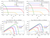Fig. 4. Spectra and light curves with Mc = 1 M⊙ (left panels) and 10 M⊙ (right panels) in a binary system with Porb = 10 d. Differently colored lines represent different mechanisms, as indicated in the legends. The blue line shows the persistent preburst radiation for Lw = 9.6 × 1044 erg s−1 corresponding to Case I, and the light blue line indicates that for Lw = 5.0 × 1034 erg s−1 corresponding to Case II. In the top panels, we show the light curves. In the bottom panels, we show the spectra for different mechanisms at a distance of d = 100 kpc. The sensitivity curves of Einstein Probe (blue line), Chandra (pink line), and XMM-Newton (black line) are calculated with an exposure time of 103 s, which can be derived from sensitivity proportional to the −1/2 power of the exposure time (Lucchetta et al. 2022; Yuan et al. 2022), and the r-band sensitivity of the Vera C. Rubin Observatory (purple line) is calculated with a point source exposure time of 30 s (Yuan et al. 2021).

In Figs. 4c and d, we show the spectra at d_L = 100 kpc with M_c = 1 M_⊙ and 10 M_⊙ for P_orb = 10 d, where d_L is the distance between the source and the observer. The persistent preburst radiation for Case I is mainly at the optical and ultraviolet (UV) bands, and that for Case II is mainly at the X-ray band and higher energy band. The re-emission from bursts is mainly at the optical, UV, and X-ray bands. We note that the re-emission from MSBs is a short process with Δt_re ∼ 0.1 in the parameter we choose, while the exposure times for the sensitivity curves shown in Figs. 4c and d are 30 s and 10³ s. The sensitivity for detectors with shorter exposure time would be lower, meaning that the re-emission from MSBs would be difficult to detect. For the optical band, the Vera C. Rubin Observatory would be capable of detecting the persistent preburst radiation with L_w ≈ 9.6 × 10⁴⁴ erg s⁻¹ (for M_c = 1 M_⊙ and 10 M_⊙) and the re-emission from MGFs (for M_c = 1 M_⊙). For the X-ray band, Einstein Probe, Chandra, and XMM-Newton cannot detect those radiations with d_L ≳ 100 kpc. However, if the distance is very close, of ∼1 kpc for example, the persistent preburst radiation produced by a bow shock might become dominant and could potentially be detected by X-ray telescopes.

3.2. Radiation properties for different parameters

In this work, we consider that a magnetar and a main sequence star are in a binary system, and analyze the radiation from the interaction between magnetar bursts and the companion star. Such binary systems are relatively common in the Universe for the following reasons: (1) The fraction of magnetars in young NSs could be about 40% based on Galactic observations (Beniamini et al. 2019), although the magnetic fields of magnetars would significantly decay after ∼(10³ − 10⁴) yr. (2) According to the catalog of Galactic X-ray binaries (Avakyan et al. 2023; Fortin et al. 2023) (see also in Table 1 of Xia et al. 2023), for a binary star system that contains a NS (likely as the central engine of FRBs) and a high-mass companion with M_c ∼ 10 − 100 M_⊙ (a low-mass companion M_c ∼ 0.1 − 7 M_⊙), the range of its orbital period is 1 − 10³ d (0.01 − 10 d). Such parameter ranges are consistent with the above discussions.

We discuss the parameter dependence of the radiation from different mechanisms including the persistent preburst radiation (blue lines and light blue lines), the re-emission from FRBs (yellow lines), MSBs (green lines), and MGFs (red lines), and the radiation from the companion itself (purple lines), as shown in Figs. 5 and 6. We show their peak luminosity in these figures, and the colored region shows the parameter space where the luminosity is larger than L_c. The blue lines show the persistent preburst radiation from the magnetar wind directly interacting with the companion (Case I), and the light blue lines represent that produced by the bow shock (Case II). The break between the blue line and the light blue line is due to the transition from Case I to Case II. We note that here d > R_c and d − R_c > d_Roche is satisfied for the parameter ranges we choose, where d_Roche ≃ R_c(2M_m/M_c)^1/3 is the distance of the Roche limit.

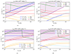Fig. 5. Comparison of the re-emission from bursts and the persistent preburst radiation with Lw = 9.6 × 1044 erg s−1 (left panels) and Lw = 5.0 × 1034 erg s−1 (right panels) for different Porb and different Mc. Different colors represent different mechanisms, as indicated in the caption. We note that we show both Case I (blue lines) and Case II (light blue lines) for the persistent preburst radiation. The colored region means νLν > Lc, where the radiation will not be outshined by Lc. In the top panel, we show the variation of the peak luminosity νLν with Mc for a given Porb = 1 and 10 d. In the bottom panel, we show the variation of νLν with Porb for a given Mc = 1 and 10 M⊙.

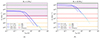Fig. 6. Persistent preburst radiation varied with the age of the magnetar corresponding to the luminosity of the magnetar wind Lw for Mc = 1 M⊙ (the left panel) and 10 M⊙ (the right panel). Similar to Fig. 5, the colored region means νLν > Lc, and differently colored lines show different mechanisms. The solid lines show the peak luminosity for Porb = 1 d, while the dashed lines show that for Porb = 10 d.

3.2.1. Radiation properties for different M_c and P_orb

In Fig. 5, we set L_w = 9.6 × 10⁴⁴ erg s⁻¹ for the typical parameters, corresponding to a newborn magnetar, and set L_w = 5.0 × 10³⁴ erg s⁻¹, which corresponds to a relatively old magnetar with T_age = 10³ yr for example. We scan the parameter space of M_c = 0.1 − 20 M_⊙ and P_orb = 1 − 1000 d.

In Figs. 5a and b, we show the peak luminosity of the radiation for M_c = 0.1 − 20 M_⊙ with P_orb = 1,  10 d. We note that the discontinuity of the solid green line represents the transition point after which the extra limitation $r_y^{\prime }-r_x^{\prime }\le c\mathrm{\Delta }{t}_{\text{burst}}$ is not satisfied and we use $r_y^{\prime }=r_x^{\prime }+c\mathrm{\Delta }{t}_{\text{burst}}$. We can see that for the companion with a small M_c ≲ 0.6 M_⊙, the re-emission from MGFs and MSBs can be larger than L_c. Only with M_c ≲ 0.21 M_⊙ and P_orb = 10 d can the re-emission from FRBs be larger than L_c. In Fig. 5a, we set L_w = 9.6 × 10⁴⁴ erg s⁻¹ corresponding to Case I. For P_orb = 1 d (10 d), the re-emission from MSBs can be greater than the persistent preburst radiation with 0.25 M_⊙ ≲ M_c ≲ 9.8 M_⊙ (M_c ≲ 2.5 M_⊙), and that from MGFs can be greater than the persistent preburst radiation with M_c ≲ 0.16 M_⊙ (0.29 M_⊙). In Fig. 5b, we use L_w = 5.0 × 10³⁴ erg s⁻¹, and the persistent preburst radiation would be outshined by the radiation from the companion itself.

In Figs. 5c and d, we show the peak luminosity for P_orb = 1 − 1000 d with M_c = 1,  10 M_⊙. We can see that νL_ν converges as P_orb increases, and the re-emission from MGFs and MSBs is greater than that from FRBs for all the selected values of P_orb. The re-emission from MGFs is larger than that from MSBs only with a relative large P_orb for M_c = 1 − 10 M_⊙. For the re-emission from FRBs (MGFs), it will be outshined by L_c with M_c = 1 − 10 M_⊙ (10 M_⊙). We note that our results do not imply that the re-emission from FRBs must be outshined, because if the transformation efficiency is higher, it has the possibility to be higher than the radiation of the companion star itself. In Fig. 5c, similar to Fig. 5a, we set L_w = 9.6 × 10⁴⁴ erg s⁻¹. For the companion with M_c = 1 M_⊙, the re-emission from MGFs (MSBs) is dominant for P_orb ≳ 440 d (≲60 d). For the companion with M_c = 10 M_⊙, the persistent preburst radiation would be dominant for all the values of P_orb we choose here, except for 5.2 d ≲ P_orb ≲ 9.2 d, where the re-emission from MSBs is dominant. In Fig. 5d, similar to Fig. 5b, the re-emission from MSBs and MGFs would be greater than the persistent preburst radiation with all the P_orb we choose.

The light blue lines in Fig. 5d show the persistent preburst radiation from the bow shock. We find that the radiation of the bow shock will change from the fast-cooling case to the slow-cooling case with increasing distance d, corresponding to increasing orbital period P_orb, and the peak flux in the slow-cooling case is inversely proportional to the distance d. As d continues to increase, there will be γ_c > γ_M, where the cooling will no longer be important, and so the radiation from the bow shock is weak.

3.2.2. Radiation properties for different L_w

According to Sect. 2, we know that the persistent preburst radiation varies with the luminosity of the magnetar wind L_w. Therefore, in Fig. 6, we show the persistent preburst radiation as a function of L_w, and compare it with the re-emission from bursts and the companion itself. For M_c = 1 M_⊙, we find the persistent preburst radiation would be larger than L_c with T_age ≲ 36 yr (8.9 yr) for P_orb = 1 d (10 d). The persistent preburst radiation would be smaller than that of the re-emission from MSBs with all the values of T_age we choose for P_orb = 1 − 10 d. The re-emission from MGFs can be larger than the persistent preburst radiation with T_age ≳ 5.6 yr for P_orb = 10 d, and the other re-emission would be outshined by L_c. For M_c = 10 M_⊙, the persistent preburst radiation will be larger than L_c with T_age ≲ 8.9 yr (2.8 yr) for P_orb = 1 d (10 d). The re-emission from MSBs will be larger than the persistent preburst radiation with all the values of T_age we choose for P_orb = 10 d, and the other re-emission is outshined by L_c.

4. Summary and discussion

In this work, we studied the radiation processes from the interaction between magnetar bursts and the main sequence star (the companion) in a binary system. We considered the possible radiation generated by the magnetar wind interacting with the companion, or the companion wind as the background of the re-emission from bursts (including FRBs, MSBs, and MGFs) interacting with the companion. For the persistent preburst radiation, we considered two possible scenarios based on L_w. For a magnetar wind with a relatively small L_w, the magnetar wind will interact with the companion wind, generating the bow shock; whereas for a magnetar wind with a large L_w, it will directly interact with the companion itself.

We calculated the spectra and light curves for the companion with M_c = 1 M_⊙ and 10 M_⊙ in a binary system with P_orb = 10 d. We find that only when the luminosity of the magnetar wind is relatively large – for example, 9.6 × 10⁴⁴ erg s⁻¹, corresponding to a newborn magnetar with P₀ = 10⁻² s and B_⊥ = 10¹⁵ G – can the persistent preburst radiation be outshined by L_c, and this mainly happens at optical and UV bands. The re-emission from MGFs with M_c = 1 M_⊙ is slightly larger than that of L_c, the re-emission from MSBs with M_c = 1 − 10 M_⊙ is ∼1 − 4 orders of magnitude larger than that of L_c, and that from FRBs with M_c = 1 − 10 M_⊙ is outshined by L_c. We note that the re-emission from FRBs with a larger transformation efficiency η could still potentially be observed. The re-emission from the bursts is mainly at the optical, UV, and X-ray bands, with a duration of ∼0.1 − 10⁵ s. For the optical band, we find that the Vera C. Rubin Observatory can detect the persistent preburst radiation with M_c = 1 − 10 M_⊙ and the re-emission from MGFs with M_c = 1 M_⊙. For the X-ray band, Einstein Probe, Chandra, and XMM-Newton cannot detect the radiations we study with d_L ≳ 100 kpc. However, in the high-energy band ≳10¹⁷ Hz, the persistent preburst radiation produced by a bow shock can become dominant, and could potentially be detected when the distance is very close ∼1 kpc.

We also scanned the parameter space of M_c, P_orb, and L_w to find which mechanism is dominant, and we find that the persistent preburst radiation and the re-emission from bursts can be larger than the radiation from the companion itself with a suitable parameter. Also, the re-emission from FRBs, MSBs, and MGFs can be greater than the persistent preburst radiation for a relatively old magnetar. For FRBs, when M_c ≲ 0.2 M_⊙, its re-emission can be greater than L_c and the persistent preburst radiation of L_w ≈ 5.0 × 10³⁴ erg s⁻¹ with P_orb = 10 d. For MSBs and MGFs, their re-emission can be larger than L_c and the persistent preburst radiation of L_w ≈ 5.0 × 10³⁴ erg s⁻¹ with M_c ≲ 0.6  M_⊙. For the persistent preburst radiation with L_w ≈ 9.6 × 10⁴⁴ erg s⁻¹, which corresponds to a newborn magnetar with P₀ = 10⁻² s and B_⊥ = 10¹⁵ G, it would be dominant with a relatively large M_c (≳1 − 10 M_⊙) and a moderate P_orb (∼10 − 100 d). We note that here we compare the peak luminosity for each radiation mechanism, and in addition to the persistent preburst radiation produced by the bow shock (Case II), the other radiation mechanism is the black-body radiation. Therefore, in high-energy bands, such as X-ray and γ-ray bands, the persistent preburst radiation produced by a bow shock might become dominant.

In the above calculations, we focus on the two main radiations, including the persistent preburst radiation from the magnetar wind and the re-emission from bursts. However, there are some additional mechanisms, including the IC scattering process between the electrons in the magnetar wind and the photons from the re-emission, and the pair annihilation from the electrons in the companion and the positrons in the magnetar wind (some details of these processes are discussed in the appendix). We find the peak luminosity from the re-emission can be scattered to a larger frequency with the IC scattering process. We also find that the pair annihilation would exist, but the photons generated by this process would be scattered by the particles in the companion star due to the optically thick surface of the companion, which cannot be detected.

Acknowledgments

We thank the anonymous referee for helpful comments to improve this paper. We thank the helpful discussions with Bing Zhang, Jia Ren, and Fa-Yin Wang, and we thank the useful information given by Xin-Lian Luo, Yue Wu, Bo-Yang Liu, Zhen-Yin Zhao, Qian-Qian Zhang, and Lu-yao Jiang. D.M.W. is supported by the National Natural Science Foundation of China (No. 11933010, 11921003, 12073080, 12233011) and the Strategic Priority Research Program of the Chinese Academy of Sciences (grant No. XDB0550400). Z.G.D. is supported by the National SKA Program of China (grant No. 2020SKA0120300) and National Natural Science Foundation of China (grant No. 12393812). Y.P.Y. is supported by the National Natural Science Foundation of China grant No.12003028 and the National SKA Program of China (2022SKA0130100).

References

Appendix A: Pair annihilation between electrons in companion and positrons in relativistic wind

The pair annihilation is one of the possible heating mechanisms due to the very high density of the electrons in the companion, in which an electron (from the companion) and a positron (from the magnetar wind) annihilate, resulting in the creation of two photons. The cross section for this process is (Jauch & Rohrlich 1976)

$$\begin{array}{c}\hfill \begin{array}{cc}& {\sigma }_{e^{+}{e}^{-}}=\frac{\pi r_0^2}{{\gamma }_{\mathrm{w}}+1}[\frac{{\gamma }_{\mathrm{w}}^2+4{\gamma }_{\mathrm{w}}+1}{{\gamma }_{\mathrm{w}}^2-1}\ln ({\gamma }_{\mathrm{w}}+\sqrt{{\gamma }_{\mathrm{w}}^2-1})-\frac{{\gamma }_{\mathrm{w}}+3}{\sqrt{{\gamma }_{\mathrm{w}}^2-1}}].\hfill \end{array}\end{array}$$(A.1)

The corresponding optical depth τ_e⁺e⁻ ∼ n_cσ_e⁺e⁻r_b can be calculated, where n_c ≃ ρ_c/m_p is the number density of electrons in the companion. The optical depth can be much larger than 1 due to the large n_c, as shown in the blue line in Fig. A.1, which means that the possibility of pair annihilation would be large and the radiation from this process cannot be neglected. However, the emitting photons might be scattered by the particles in the companion star due to the optically thick companion surface. We then calculate the corresponding optical depth τ_T ∼ κρ_cl(θ), considering the Thomson scattering, where l(θ) is the length of the companion star at a given θ_m (θ_m is the angle between the line connecting the two stars and the line connecting the magnetar and the point we studied). The descriptions of θ_m and θ_m2 are presented in Fig. 2. According to the red line in Fig. A.1, we can see that the radiation could only be potentially observed with a θ_m of around θ_m2 ≈ 0.038 rad (where τ_T < 1). Therefore, the radiation from the pair annihilation can be neglected, and it contributes to the heating of the companion star by the magnetar wind.

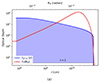Fig. A.1. Optical depth for a solar-like companion with Mc = 1 M⊙. The blue line shows the optical depth for the pair annihilation at different radii, and the colored region means τe+e− > 1. The red line represents the optical depth of absorption at various viewing angles θm ∈ (0, θm2). The corresponding parameters we used are γw = 104 and Porb = 10 d.

Appendix B: Inverse Compton between electrons in relativistic wind and photons from re-emission

The inverse Compton (IC) scattering process may also take place between the electrons in the relativistic wind and the photons from the re-emission. The IC spectrum for isotropic electrons and isotropic photons at a₁ = hν₁/(m_ec²) (where ν₁ is the emitting photon frequency) should be (Blumenthal & Gould 1970)

$$\begin{array}{c}\hfill \begin{array}{cc}& L_{\mathrm{IC}}\sim {\nu }_1{L}_{{\nu }_1}=V_{\mathrm{IC}}h{\nu }_1^2\int \int n_{\mathrm{e}}(\gamma )n_{\mathrm{ph}}(\nu )\frac{d{N}_{\gamma ,\nu }}{dtd{\nu }_1}d\nu d\gamma ,\hfill \\ \hfill & \frac{d{N}_{\gamma ,\nu }}{dtd{\nu }_1}=\frac{2\pi r_0^{2}c}{\nu {\gamma }^2}[2q\ln q+(1+2q)(1-q)+\frac{1-q}{2}\frac{{(4a_1\gamma q)}^2}{1+4a_1\gamma q}],\hfill \end{array}\end{array}$$(B.1)

where $q=\frac{{(a_1/\gamma )}^2}{4a{a}_1(1-a_1/\gamma )}$ is a dimensionless parameter, r₀ = e²/(m_ec²) is the classical electron radius, and $n_{\mathrm{e}}(\gamma )=n_{e,0}(1-p)\frac{{\gamma }^{-p}}{{\gamma }_{\mathrm{M}}^{-p+1}-{\gamma }_{\mathrm{m}}^{-p+1}},{\gamma }_{\mathrm{m}}<\gamma <{\gamma }_{\mathrm{M}}$ is the differential number density of the power-law distribution electrons contributed by the magnetar wind. We take the photons produced by the persistent preburst radiation for Case I as the seed photon for example. We use P_w = P_re to estimate the width of the interaction region (where P_re ≃ L_re/(12πδr²c) is the radiation pressure), which is $\delta r\sim (a-R_{\mathrm{c}})/(1+\sqrt{L_{\mathrm{w}}/L_{\mathrm{re}}})$, as shown in Fig. 2a. We then approximate that the volume of the interaction region is $V_{\text{IC}}~\pi \delta r{R}_{\text{c}}^2$, and the number density of the photons is n_ph(ν) = L_ν/(4πhν(R_c + δr)²c). We note that n_{e,0 ≃ Ṅ/(4π(a − Rc)²c}) is the number density for power-law distribution electrons, where $\dot{N}\simeq \frac{L_{\mathrm{w}}}{m_{\mathrm{e}}{c}^2}\frac{2-p}{1-p}\frac{{\gamma }_{\mathrm{M}}^{-p+1}-{\gamma }_{\mathrm{m}}^{-p+1}}{{\gamma }_{\mathrm{M}}^{-p+2}-{\gamma }_{\mathrm{m}}^{-p+2}}$ is the number of electrons per second at a − R_c.

In Fig. B.1, we consider the case where the seed photon for the IC process is mainly from the persistent preburst radiation generated by Case I. Here we take the solar-like companion with M_c = 1 M_⊙ and the newborn magnetar corresponding to L_w ≈ 9.6 × 10⁴⁴ erg s⁻¹ (the magnetar with T_age = 10² yr corresponding to L_w ≈ 5.0 × 10³⁶ erg s⁻¹) for example. We find that the peak luminosity for the persistent preburst radiation can be scattered to a large frequency. For T_age = 10² yr, the peak luminosity for the IC spectrum is ≈ 1.3 × 10²⁴ erg s⁻¹ at ν ≈ 6.9 × 10²¹ Hz. For a newborn magnetar, the peak luminosity for IC is ≈ 3.8 × 10³⁵ erg s⁻¹ at ν ≈ 1.2 × 10²³ Hz, which is similar to that for the persistent preburst radiation due to the large number density of electrons. Considering the possible two-photon pair production process between the photons from the IC scattering process (ν_IC) and the lower energy photons (ν_seed), the frequency of the lower energy photons should satisfy ${\nu }_{\mathrm{seed}}\ge {(m_{\mathrm{e}}{c}^2/h)}^2{\nu }_{\mathrm{IC}}^{-1}\simeq 1.3\times {10}^{17}\mathrm{Hz}{\nu }_{\mathrm{IC},24}^{-1}$, which is much larger than the peak frequency of the radiation from the solar-like companion itself ≈3.4 × 10¹⁴ Hz with T_c,eff ≈ 5770 K. In this way, here we neglect this effect. For Case II of the persistent preburst radiation, the IC scattering process can also scatter the seed photons to a relatively high frequency of ∼ 10²⁴ Hz.

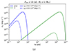Fig. B.1. Spectra of the persistent preburst radiation for Case I involving the IC process with Tage = 102 yr corresponding to Lw ≃ 5.0 × 1036 erg s−1 (the dashed line) and Tage = 0 yr corresponding to Lw ≃ 9.6 × 1044 erg s−1 (the solid line). We set Porb = 10 day, corresponding to a ≈ 3.9 × 1011 cm and Mc = 1 M⊙. The blue lines show the preburst radiation spectrum of Case I. The green line indicates the IC spectrum. The corresponding parameters we used are p = 2.2, γm = 104, and γM = 106.

In addition, we investigate the impact of the repeated scatterings involving relativistic electrons in purely scattering scenarios, by calculating the Compton Y parameter (Rybicki & Lightman 1985)

$$\begin{array}{c}\hfill Y\simeq \frac{64}{3}\langle {\gamma }^2\rangle max({\tau }_{\mathrm{es}},{\tau }_{\mathrm{es}}^2),\end{array}$$(B.2)

where τ_es = ρ_eκδr is the scattering optical depth, and ρ_e = m_en_e is the density of the electrons. We find that the value of Y is about 4.8 × 10⁻⁵ (4.1 × 10⁻³) for the magnetar with T_age = 10³ yr (the newborn magnetar), which is smaller than 1, indicating that the repeated scattering process is not important.

All Figures

Fig. 1. Schematic picture of radiation generated by a burst and/or a wind from a magnetar interacting with a main sequence star in a binary system. The persistent preburst radiation is generated by a strong magnetar wind heating a companion star, or by the bow shock from a weak magnetar wind interacting with a stellar wind from a companion star. The radiation from the transient is generated by the re-emission process from the companion star heated by a magnetar burst (e.g., an FRB, an MSB, and/or an MGF).

In the text

	Fig. 2. Schematic picture of the persistent preburst radiation. In the top panel, we show the scenario (Case I) where the magnetar wind directly interacts with the companion star. In the bottom panel, we indicate the scenario (Case II) where the bow shock is generated by the interaction between the magnetar wind and the possible strong companion wind.
In the text

Fig. 3. Permitted luminosity of the magnetar wind and the corresponding age of the magnetar for a given Mc which varies from 0.1 M⊙ to 100 M⊙, at which the magnetar wind will interact with the companion wind with the generation of the bow shock. Different colors represent different values of Porb, as indicated in the caption. The solid lines show the luminosity of the magnetar wind, while the dashed lines indicate the age of the magnetar. The colored areas show the permitted parameter for the scenario where the bow shock is generated from the interaction between the magnetar wind and the companion wind.

In the text

Fig. 4. Spectra and light curves with Mc = 1 M⊙ (left panels) and 10 M⊙ (right panels) in a binary system with Porb = 10 d. Differently colored lines represent different mechanisms, as indicated in the legends. The blue line shows the persistent preburst radiation for Lw = 9.6 × 1044 erg s−1 corresponding to Case I, and the light blue line indicates that for Lw = 5.0 × 1034 erg s−1 corresponding to Case II. In the top panels, we show the light curves. In the bottom panels, we show the spectra for different mechanisms at a distance of d = 100 kpc. The sensitivity curves of Einstein Probe (blue line), Chandra (pink line), and XMM-Newton (black line) are calculated with an exposure time of 103 s, which can be derived from sensitivity proportional to the −1/2 power of the exposure time (Lucchetta et al. 2022; Yuan et al. 2022), and the r-band sensitivity of the Vera C. Rubin Observatory (purple line) is calculated with a point source exposure time of 30 s (Yuan et al. 2021).

In the text

Fig. 5. Comparison of the re-emission from bursts and the persistent preburst radiation with Lw = 9.6 × 1044 erg s−1 (left panels) and Lw = 5.0 × 1034 erg s−1 (right panels) for different Porb and different Mc. Different colors represent different mechanisms, as indicated in the caption. We note that we show both Case I (blue lines) and Case II (light blue lines) for the persistent preburst radiation. The colored region means νLν > Lc, where the radiation will not be outshined by Lc. In the top panel, we show the variation of the peak luminosity νLν with Mc for a given Porb = 1 and 10 d. In the bottom panel, we show the variation of νLν with Porb for a given Mc = 1 and 10 M⊙.

In the text

Fig. 6. Persistent preburst radiation varied with the age of the magnetar corresponding to the luminosity of the magnetar wind Lw for Mc = 1 M⊙ (the left panel) and 10 M⊙ (the right panel). Similar to Fig. 5, the colored region means νLν > Lc, and differently colored lines show different mechanisms. The solid lines show the peak luminosity for Porb = 1 d, while the dashed lines show that for Porb = 10 d.

In the text

	Fig. A.1. Optical depth for a solar-like companion with Mc = 1 M⊙. The blue line shows the optical depth for the pair annihilation at different radii, and the colored region means τe+e− > 1. The red line represents the optical depth of absorption at various viewing angles θm ∈ (0, θm2). The corresponding parameters we used are γw = 104 and Porb = 10 d.
In the text

Fig. B.1. Spectra of the persistent preburst radiation for Case I involving the IC process with Tage = 102 yr corresponding to Lw ≃ 5.0 × 1036 erg s−1 (the dashed line) and Tage = 0 yr corresponding to Lw ≃ 9.6 × 1044 erg s−1 (the solid line). We set Porb = 10 day, corresponding to a ≈ 3.9 × 1011 cm and Mc = 1 M⊙. The blue lines show the preburst radiation spectrum of Case I. The green line indicates the IC spectrum. The corresponding parameters we used are p = 2.2, γm = 104, and γM = 106.

In the text

References

- Archibald, R. F., Kaspi, V. M., Beardmore, A. P., Gehrels, N., & Kennea, J. A. 2015, ApJ, 810, 67 [NASA ADS] [CrossRef] [Google Scholar]
- Avakyan, A., Neumann, M., Zainab, A., et al. 2023, A&A, 675, A199 [NASA ADS] [CrossRef] [EDP Sciences] [Google Scholar]
- Badenes, C., Mazzola, C., Thompson, T. A., et al. 2018, ApJ, 854, 147 [NASA ADS] [CrossRef] [Google Scholar]
- Beloborodov, A. M. 2013, ApJ, 762, 13 [NASA ADS] [CrossRef] [Google Scholar]
- Beniamini, P., Hotokezaka, K., van der Horst, A., & Kouveliotou, C. 2019, MNRAS, 487, 1426 [NASA ADS] [CrossRef] [Google Scholar]
- Beniamini, P., Wadiasingh, Z., Hare, J., et al. 2023, MNRAS, 520, 1872 [CrossRef] [Google Scholar]
- Bhardwaj, M., Gaensler, B. M., Kaspi, V. M., et al. 2021, ApJ, 910, L18 [NASA ADS] [CrossRef] [Google Scholar]
- Bhattacharya, D., & van den Heuvel, E. 1991, Phys. Rep., 203, 1 [NASA ADS] [CrossRef] [Google Scholar]
- Blumenthal, G. R., & Gould, R. J. 1970, Rev. Mod. Phys., 42, 237 [Google Scholar]
- Bochenek, C. D., Ravi, V., Belov, K. V., et al. 2020, Nature, 587, 59 [NASA ADS] [CrossRef] [Google Scholar]
- Bozzo, E., Ferrigno, C., Oskinova, L., & Ducci, L. 2022, MNRAS, 510, 4645 [NASA ADS] [CrossRef] [Google Scholar]
- Breton, R. P., Kaspi, V. M., McLaughlin, M. A., et al. 2012, ApJ, 747, 89 [NASA ADS] [CrossRef] [Google Scholar]
- Bucciantini, N., Amato, E., & Del Zanna, L. 2005, A&A, 434, 189 [NASA ADS] [CrossRef] [EDP Sciences] [Google Scholar]
- Burns, E., Svinkin, D., Hurley, K., et al. 2021, ApJ, 907, L28 [NASA ADS] [CrossRef] [Google Scholar]
- Cantó, J., Raga, A. C., & Wilkin, F. P. 1996, ApJ, 469, 729 [Google Scholar]
- Chen, A. Y., & Beloborodov, A. M. 2017, ApJ, 844, 133 [NASA ADS] [CrossRef] [Google Scholar]
- Chen, A. M., Takata, J., Yi, S. X., Yu, Y. W., & Cheng, K. S. 2019, A&A, 627, A87 [NASA ADS] [CrossRef] [EDP Sciences] [Google Scholar]
- Chen, A. M., Guo, Y. D., Yu, Y. W., & Takata, J. 2021, A&A, 652, A39 [NASA ADS] [CrossRef] [EDP Sciences] [Google Scholar]
- Chen, P., Gal-Yam, A., Sollerman, J., et al. 2024, Nature, 625, 253 [NASA ADS] [CrossRef] [Google Scholar]
- CHIME/FRB Collaboration (Andersen, B. C., et al.) 2020, Nature, 587, 54 [Google Scholar]
- Chrimes, A. A., Levan, A. J., Fruchter, A. S., et al. 2022, MNRAS, 513, 3550 [NASA ADS] [CrossRef] [Google Scholar]
- Cline, T. L., Desai, U., Mushotzky, R., et al. 1980, Bull. Am. Astron. Soc., 12, 448 [Google Scholar]
- Cline, T. L., Desai, U. D., Teegarden, B. J., et al. 1982, ApJ, 255, L45 [NASA ADS] [CrossRef] [Google Scholar]
- Cook, G. B., Shapiro, S. L., & Teukolsky, S. A. 1994, ApJ, 422, 227 [CrossRef] [Google Scholar]
- Coroniti, F. V. 1990, ApJ, 349, 538 [Google Scholar]
- Dai, Z. G. 2004, ApJ, 606, 1000 [NASA ADS] [CrossRef] [Google Scholar]
- Daugherty, J. K., & Harding, A. K. 1983, ApJ, 273, 761 [Google Scholar]
- Dermer, C. D. 1990, ApJ, 360, 197 [CrossRef] [Google Scholar]
- Duchêne, G., & Kraus, A. 2013, ARA&A, 51, 269 [Google Scholar]
- Esposito, P., Rea, N., Borghese, A., et al. 2020, ApJ, 896, L30 [NASA ADS] [CrossRef] [Google Scholar]
- Fortin, F., García, F., Simaz Bunzel, A., & Chaty, S. 2023, A&A, 671, A149 [NASA ADS] [CrossRef] [EDP Sciences] [Google Scholar]
- Geng, J. J., Wu, X. F., Huang, Y. F., Li, L., & Dai, Z. G. 2016, ApJ, 825, 107 [NASA ADS] [CrossRef] [Google Scholar]
- Granot, J., Ramirez-Ruiz, E., Taylor, G. B., et al. 2006, ApJ, 638, 391 [CrossRef] [Google Scholar]
- Guenther, D. B., Demarque, P., Kim, Y. C., & Pinsonneault, M. H. 1992, ApJ, 387, 372 [CrossRef] [Google Scholar]
- H.E.S.S. Collaboration (Abdalla, H., et al.) 2022, in 37th International Cosmic Ray Conference, 777 [Google Scholar]
- Hirai, R., Podsiadlowski, P., & Yamada, S. 2018, ApJ, 864, 119 [NASA ADS] [CrossRef] [Google Scholar]
- Hu, C.-P., Begiçarslan, B., Güver, T., et al. 2020, ApJ, 902, 1 [NASA ADS] [CrossRef] [Google Scholar]
- Iben, I. 2012, Stellar Evolution Physics, Volume 1: Physical Processes in Stellar Interiors (Cambridge University Press) [Google Scholar]
- Israel, G. L., Esposito, P., Rea, N., et al. 2016, MNRAS, 457, 3448 [NASA ADS] [CrossRef] [Google Scholar]
- Jauch, J. M., & Rohrlich, F. 1976, The Theory of Photons and Electrons. The Relativistic Quantum Field Theory of Charged Particles with Spin One-half (New York: Springer) [Google Scholar]
- Kasen, D. 2010, ApJ, 708, 1025 [Google Scholar]
- Kasen, D., & Bildsten, L. 2010, ApJ, 717, 245 [NASA ADS] [CrossRef] [Google Scholar]
- Kaspi, V. M., & Beloborodov, A. M. 2017, ARA&A, 55, 261 [Google Scholar]
- Kennel, C. F., & Coroniti, F. V. 1984a, ApJ, 283, 694 [CrossRef] [Google Scholar]
- Kennel, C. F., & Coroniti, F. V. 1984b, ApJ, 283, 710 [Google Scholar]
- Kirk, J. G., & Skjæraasen, O. 2003, ApJ, 591, 366 [CrossRef] [Google Scholar]
- Kong, S. W., Yu, Y. W., Huang, Y. F., & Cheng, K. S. 2011, MNRAS, 416, 1067 [NASA ADS] [CrossRef] [Google Scholar]
- Koranda, S., Stergioulas, N., & Friedman, J. L. 1997, ApJ, 488, 799 [NASA ADS] [CrossRef] [Google Scholar]
- Kouveliotou, C., Dieters, S., Strohmayer, T., et al. 1998, Nature, 393, 235 [NASA ADS] [CrossRef] [Google Scholar]
- Kremer, K., Piro, A. L., & Li, D. 2021, ApJ, 917, L11 [NASA ADS] [CrossRef] [Google Scholar]
- Kuiper, L., Hermsen, W., & Dekker, A. 2018, MNRAS, 475, 1238 [NASA ADS] [CrossRef] [Google Scholar]
- Lang, K. R. 1999, Astrophysical Formulae (New York: Springer) [CrossRef] [Google Scholar]
- Lee, W. H., Ramirez-Ruiz, E., & van de Ven, G. 2010, ApJ, 720, 953 [CrossRef] [Google Scholar]
- Lin, L., Göğüş, E., Roberts, O. J., et al. 2020, ApJ, 893, 156 [CrossRef] [Google Scholar]
- Lucchetta, G., Ackermann, M., Berge, D., & Bühler, R. 2022, J. Cosmol. Astropart. Phys., 2022, 013 [CrossRef] [Google Scholar]
- Luo, D., McCray, R., & Mac Low, M.-M. 1990, ApJ, 362, 267 [CrossRef] [Google Scholar]
- Luo, R., Men, Y., Lee, K., et al. 2020, MNRAS, 494, 665 [NASA ADS] [CrossRef] [Google Scholar]
- Maan, Y., Leeuwen, J. V., Straal, S., & Pastor-Marazuela, I. 2022, ATel, 15697, 1 [NASA ADS] [Google Scholar]
- MacFadyen, A. I., Ramirez-Ruiz, E., & Zhang, W. 2005, ArXiv e-prints [arXiv:astro-ph/0510192] [Google Scholar]
- Mazets, E. P., Golentskii, S. V., Ilinskii, V. N., Aptekar, R. L., & Guryan, I. A. 1979, Nature, 282, 587 [NASA ADS] [CrossRef] [Google Scholar]
- Medin, Z., & Lai, D. 2010, MNRAS, 406, 1379 [NASA ADS] [Google Scholar]
- Mereghetti, S. 2008, A&A Rev., 15, 225 [NASA ADS] [CrossRef] [Google Scholar]
- Mereghetti, S., Rigoselli, M., Salvaterra, R., et al. 2024, Nature, 629, 58 [NASA ADS] [CrossRef] [Google Scholar]
- Minaev, P. Y., & Pozanenko, A. S. 2020, Astron. Lett., 46, 573 [NASA ADS] [CrossRef] [Google Scholar]
- Murase, K., Mészáros, P., & Fox, D. B. 2017, ApJ, 836, L6 [NASA ADS] [CrossRef] [Google Scholar]
- Nadyozhin, D. K., & Razinkova, T. L. 2005, Astron. Lett., 31, 695 [CrossRef] [Google Scholar]
- Olausen, S. A., & Kaspi, V. M. 2014, ApJS, 212, 6 [Google Scholar]
- Palmer, D. M., & Swift/BAT Team 2022, ATel, 15752, 1 [NASA ADS] [Google Scholar]
- Pavlović, M. Z., Urošević, D., Vukotić, B., Arbutina, B., & Göker, Ü. D. 2013, ApJS, 204, 4 [CrossRef] [Google Scholar]
- Rees, M. J., & Gunn, J. E. 1974, MNRAS, 167, 1 [CrossRef] [Google Scholar]
- Roberts, O. J., Veres, P., Baring, M. G., et al. 2021, Nature, 589, 207 [NASA ADS] [CrossRef] [Google Scholar]
- Rybicki, G. B., & Lightman, A. P. 1985, Radiative Processes in Astrophysics (Wiley-VCH) [CrossRef] [Google Scholar]
- Salaris, M., & Cassisi, S. 2005, Evolution of Stars and Stellar Populations (Wiley-VCH) [Google Scholar]
- Sefako, R. R., & de Jager, O. C. 2003, ApJ, 593, 1013 [CrossRef] [Google Scholar]
- Shibata, S., Tomatsuri, H., Shimanuki, M., Saito, K., & Mori, K. 2003, MNRAS, 346, 841 [CrossRef] [Google Scholar]
- Stratta, G., Dainotti, M. G., Dall’Osso, S., Hernandez, X., & De Cesare, G. 2018, ApJ, 869, 155 [NASA ADS] [CrossRef] [Google Scholar]
- Svinkin, D., Frederiks, D., Hurley, K., et al. 2021, Nature, 589, 211 [NASA ADS] [CrossRef] [Google Scholar]
- Tavani, M., & Arons, J. 1997, ApJ, 477, 439 [NASA ADS] [CrossRef] [Google Scholar]
- Tavani, M., Casentini, C., Ursi, A., et al. 2021, Nat. Astron., 5, 401 [NASA ADS] [CrossRef] [Google Scholar]
- Thompson, C. 2008, ApJ, 688, 499 [NASA ADS] [CrossRef] [Google Scholar]
- Thompson, C., & Duncan, R. C. 1993, ApJ, 408, 194 [NASA ADS] [CrossRef] [Google Scholar]
- Thompson, C., & Duncan, R. C. 1996, ApJ, 473, 322 [NASA ADS] [CrossRef] [Google Scholar]
- Tonks, L., & Langmuir, I. 1929, Phys. Rev., 33, 195 [NASA ADS] [CrossRef] [Google Scholar]
- Usov, V. V. 1984, Ap&SS, 107, 191 [Google Scholar]
- Usov, V. V. 1992, ApJ, 389, 635 [Google Scholar]
- van der Merwe, C. J. T., Wadiasingh, Z., Venter, C., Harding, A. K., & Baring, M. G. 2020, ApJ, 904, 91 [Google Scholar]
- Vink, J. S., de Koter, A., & Lamers, H. J. G. L. M. 2000, A&A, 362, 295 [Google Scholar]
- Wadiasingh, Z., Harding, A. K., Venter, C., Böttcher, M., & Baring, M. G. 2017, ApJ, 839, 80 [NASA ADS] [CrossRef] [Google Scholar]
- Wang, Y., Wei, Y.-J., Zhou, H., et al. 2024, ApJ, 969, 127 [NASA ADS] [CrossRef] [Google Scholar]
- Wilkin, F. P. 1996, ApJ, 459, L31 [Google Scholar]
- Wood, B. E., Müller, H.-R., Zank, G. P., & Linsky, J. L. 2002, ApJ, 574, 412 [NASA ADS] [CrossRef] [Google Scholar]
- Xia, Z.-Y., Yang, Y.-P., Li, Q.-C., et al. 2023, ApJ, 957, 1 [CrossRef] [Google Scholar]
- Xu, K., Li, X.-D., Cui, Z., et al. 2022, RAA, 22, 015005P [Google Scholar]
- Yang, Y.-P. 2021, ApJ, 920, 34 [CrossRef] [Google Scholar]
- Yang, Y.-P., & Zhang, B. 2021, ApJ, 919, 89 [NASA ADS] [CrossRef] [Google Scholar]
- Yang, J., Chand, V., Zhang, B.-B., et al. 2020, ApJ, 899, 106 [NASA ADS] [CrossRef] [Google Scholar]
- Younes, G., Güver, T., Kouveliotou, C., et al. 2020, ApJ, 904, L21 [CrossRef] [Google Scholar]
- Younes, G., Enoto, T., Hu, C.-P., et al. 2022, ATel, 15674, 1 [NASA ADS] [Google Scholar]
- Yuan, C., Murase, K., Zhang, B. T., Kimura, S. S., & Mészáros, P. 2021, ApJ, 911, L15 [NASA ADS] [CrossRef] [Google Scholar]
- Yuan, W., Zhang, C., Chen, Y., & Ling, Z. 2022, Handbook of X-ray and Gamma-ray Astrophysics, 86 [Google Scholar]
- Zabalza, V., Bosch-Ramon, V., Aharonian, F., & Khangulyan, D. 2013, A&A, 551, A17 [NASA ADS] [CrossRef] [EDP Sciences] [Google Scholar]
- Zhang, B. -B., Zhang, Z. J., Zou, J. -H., et al. 2022, ArXiv e-prints [arXiv:2205.07670] [Google Scholar]
- Zhong, S.-Q., Dai, Z.-G., Zhang, H.-M., & Deng, C.-M. 2020, ApJ, 898, L5 [NASA ADS] [CrossRef] [Google Scholar]
- Zhou, P., Zhou, X., Chen, Y., et al. 2020, ApJ, 905, 99 [NASA ADS] [CrossRef] [Google Scholar]
- Zou, Z.-C., Zhang, B.-B., Huang, Y.-F., & Zhao, X.-H. 2021, ApJ, 921, 2 [NASA ADS] [CrossRef] [Google Scholar]