© The Authors 2025

1. Introduction

Fast radio bursts (FRBs) are extremely-bright millisecond pulses discovered in 2007 (Lorimer et al. 2007). Due to the dedicated search for bursts from different radio facilities in the past a few years, more than eight hundred FRB events are discovered and several tens of them are repeating. With the rapidly-accumulating sample of events and bursts, our understanding on this mysterious phenomenon is being refreshed continuously (for recent reviews, see e.g., Xiao et al. 2021; Petroff et al. 2022; Zhang 2023). The Five-hundred-meter Aperture Spherical Telescope (FAST) is suitable for performing long-time monitoring of these repeaters. Thanks to its high sensitivity, the fine characterization of several repeaters has been achieved, with burst counts reaching the level of a thousand.

One of the most interesting findings by FAST is that the dynamic magnetic environment indicated by long-term rotation measure (RM) evolution. Oscillating RM variation was firstly discovered in FRB 20201124A (Xu et al. 2022) and then confirmed in FRB 20190520B, even with a sign reversal (Anna-Thomas et al. 2023). This oscillation behavior was suggested to originate from a binary system consists of a neutron star (NS) and a massive star (Wang et al. 2022). With the orbital motion of the FRB-emitting NS through the magnetized disk or wind of the massive star, significant RM variation is induced then the RM oscillation period is determined by the orbital period (Zhao et al. 2023). This picture remains to be tested since there is no concrete evidence of multiple periods.

The very recent discovery in FRB 20220529 is more intriguing that a sudden increase of RM was identified. For over 17 months, its RM varied slowly between −300 and 300 rad m⁻², however, it encountered an abrupt boost to 1976.9 rad m⁻² within the next two months and recovered to normal level in just 14 days (Li et al. 2025). A long-term DM fluctuation of ∼20 pc cm⁻³ is also seen, but it is quite stochastic and not closely related to the RM variation. In particular, the observed DM variation during the abrupt RM change phase is quite small compared to its stochastic fluctuation. This rapid change of RM indicates that some kind of magnetized plasma appeared along the line of sight. The short recovery time has suggested a short existence time of this plasma. In the binary scenario, it is likely that the massive star ejected some coronal plasma due to a stellar flare. Alternatively, the magnetar itself can also eject ionized plasma during a flare. In this work, I focus on this magnetar flare scenario.

The source of FRBs is still on debate but magnetar model is in the leading position since the solid association between an X-ray burst from Galactic magnetar SGR 1935+2154 with FRB 20200428D (CHIME/FRB Collaboration 2020; Bochenek et al. 2020; Li et al. 2021; Mereghetti et al. 2020; Ridnaia et al. 2021; Tavani et al. 2021). It is well established that magnetar giant flares are capable of ejecting huge amount of baryons, for instance, an outflow mass of ≥10^24.5 g for SGR 1806−20 giant flare was confirmed by radio observation (Gelfand et al. 2005). As a scaled-down version of giant flare, it is expected that some baryonic plasma was also ejected during normal magnetar flares. Theoretically, baryons in the crust can be ejected via magnetic reconnection induced by starquake or slow untwisting of the internal magnetic field (Thompson & Duncan 1995; Lyutikov 2003). Observationally, one possible piece of indirect evidence could come from the fact that the persistent radio source of FRB 20121102A and its huge RM are consistent with a flaring magnetar embedded in a wind nebula (Margalit & Metzger 2018). In this case, sufficient ions are needed since pure pair plasma contributes no net RM. However, an X-ray burst forest was detected before FRB 20200428D (Younes et al. 2020; Kaneko et al. 2021), but the RM value of this FRB is similar to those of the normal radio pulses from this magnetar (Zhu et al. 2023). This implies that the flare ejecta (if present) do not contribute to the observed RM for this FRB. This point needs to be properly addressed within magnetar flare scenario.

This Letter is organized as follows. In Section 2, I introduce a toy model for magnetar flare ejecta. Then in Section 3, I present the theoretical predictions of the model and discuss parameter dependences. Furthermore, I describe the application of our model to two special events in Section 4, where the drastic RM change of FRB 20220529 and the absence of change of FRB 20200428D are well explained. I finish with a discussion and conclusions in Section 5.

2. Toy model description

The magnetar can produce a flare and the ejecta may be heavily baryon-loaded. Ejecta matter is assumed to be composed by a bunch of shells with different velocities, as shown in Figure 1. The radial structure of the flare ejecta is assumed to be a universal power-law form, namely, the mass distribution follows

$$\begin{array}{c}\hfill \frac{\mathrm{d}M}{\mathrm{d}v}\propto v^s,\end{array}$$(1)

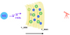Fig. 1. Schematic picture of the toy model. The ejecta are composed of several ion shells with different velocities. The mass distribution is not necessarily uniform for both the radial and angular directions.

with s ≤ 0. The normalization is determined by ${\int }_{v_{\min }}^{v_{\max }}\frac{\mathrm{d}M}{\mathrm{d}v}\mathrm{d}v=M_{\mathrm{ej}}$ where v_min,  v_max are the shell velocities at the inner and outer boundary, respectively. The angular structure of ejecta is somewhat uncertain. In general, we can introduce the latitudinal and longitudinal angles θ_ej,  φ_ej to describe it. If we assume a homologous expansion r = vt, the volume of a shell is

$$\begin{array}{c}\hfill \mathrm{d}V=rcos\theta \mathrm{d}\theta ·r\mathrm{d}\phi ·t\mathrm{d}v.\end{array}$$(2)

Introducing the shell density, ρ, we have

$$\begin{array}{c}\hfill {\int }_0^{{\phi }_{\mathrm{ej}}}{\int }_{v_{\min }}^{v_{\max }}{\int }_0^{{\theta }_{\mathrm{ej}}}2\rho cos\theta v^2{t}^3\mathrm{d}\phi \mathrm{d}v\mathrm{d}\theta =M_{\mathrm{ej}}.\end{array}$$(3)

The above expression applies to the most general case. To be more specific, we can make further assumptions on the angular structure. Similarly to the case of the structure of a gamma-ray burst jet or kilonova ejecta (e.g., Huang et al. 2018), I have assumed a simple power-law mass profile in the latitudinal direction,

$$\begin{array}{c}\hfill \frac{\mathrm{d}m}{cos\theta \mathrm{d}\theta }\propto \{\begin{array}{cc}1,\hfill & \mathrm{if}\theta \le {\theta }_c,\hfill \\ {(\frac{\theta }{{\theta }_c})}^k,\hfill & \mathrm{if}\theta >{\theta }_c,\hfill \end{array}\end{array}$$(4)

where θ_c represents the central core and dm is the mass along a certain longitudinal direction. For simplicity, I assumed the shell mass is distributed uniformly in longitudinal direction, hence, the normalization is calculated via ${\int }_0^{{\theta }_{\mathrm{ej}}}2\frac{\mathrm{d}m}{cos\theta \mathrm{d}\theta }\mathrm{d}\theta =\frac{\mathrm{d}M}{\mathrm{d}v}/{\phi }_{\mathrm{ej}}$. With these simplifications, we can easily express the shell density as

$$\begin{array}{c}\hfill \rho =\frac{\mathrm{d}m}{cos\theta \mathrm{d}\theta (v^2{t}^3)}·\end{array}$$(5)

Assuming a initially-ionized pure hydrogen ejecta with a mean molecular weight of μ_m ∼ 1 after the magnetar flare, we get the initial free electron number density: n_e, 0 = ρ/(μ_mm_p). It is reasonable to assume full ionization at the beginning since the thermal X-ray emission from the magnetar surface suggests a typical plasma temperature of the order of kT₀ ∼ keV (Kaspi & Beloborodov 2017), which is much greater than the ionization energy of hydrogen, I_H ≃ 13.6 eV. However, the shells suffer adiabatic cooling while moving outwards and the temperature decreases with radius as T ∝ r^−2/3. Once it drops close to I_H, recombination is non-negligible. The recombination coefficient is given by Burbidge et al. (1963)

$$\begin{array}{c}\hfill {\alpha }_{\mathrm{R}}(T)=2\left(\frac{32\pi }{3^{3/2}}\right){\alpha }^3{a}_0^2{\left(\frac{2kT}{\pi m_e}\right)}^{1/2}Y\varphi (Y){\overline{g}}_{\mathrm{R}},\end{array}$$(6)

where Y ≡ I_H/kT is dimensionless, α is fine structure constant, a₀ is the Bohr radius, and ${\overline{g}}_{\mathrm{R}}\sim 0.9$ is the recombination Gaunt factor. The approximated expression of ϕ(Y) is (Tucker & Gould 1966), namely,

$$\begin{array}{c}\hfill \varphi (Y)\simeq \{\begin{array}{cc}0.5[1.735+lnY+{(6Y)}^{-1}],\hfill & \mathrm{if}Y\ge 1,\hfill \\ Y(-0.298-1.202lnY),\hfill & \mathrm{if}Y\ll 1.\hfill \end{array}\end{array}$$(7)

Due to recombination, the decrement rate of number density for electrons and ions is

$$\begin{array}{c}\hfill -\frac{\mathrm{d}{n}_e}{\mathrm{d}t}=-\frac{\mathrm{d}{n}_Z}{\mathrm{d}t}={\alpha }_{\mathrm{R}}{n}_e{n}_Z.\end{array}$$(8)

For pure hydrogen ejecta Z = 1, the proton number density n_Z = n_e can be achieved at any time. We need to solve the above equation to obtain the number density of free electrons since only they are relevant to DM and RM. The dependence of contributed DM and RM by the flare ejecta with time and viewing angle is

$$\begin{array}{cc}\hfill \mathrm{DM}& ={\int }_{v_{min}}^{v_{max}}\frac{n_{e}tcos\theta }{1+z}\mathrm{d}v,\hfill \\ \hfill \mathrm{RM}& =\frac{e^3}{2\pi m_e^2{c}^4}{\int }_{v_{min}}^{v_{max}}\frac{n_e{B}_{\Vert }tcos\theta }{{(1+z)}^2}\mathrm{d}v,\hfill \end{array}$$(9)

where z is the redshift of cosmological FRBs. The parallel magnetic field strength is somewhat uncertain. Within the light cylinder radius R_LC = cP/2π, a dipole configuration is usually adopted. Generally, the field configuration outside the light cylinder can be obtained by solving an axially symmetric force-free pulsar equation for the magnetic flux (Mestel 1973; Michel 1973a; Okamoto 1974). Two of the analytic solutions found were “split monopole” (Michel 1973b) or “inclined split monopole” (Bogovalov 1999), whereby the poloidal field strength decays as B_p ∝ r⁻² and the toroidal field decays as B_φ ∝ r⁻¹. Furthermore, 3D numerical time-dependent calculations for the force-free magnetosphere of an oblique rotator were performed and the “universal solution” was found (Spitkovsky 2006; Kalapotharakos & Contopoulos 2009). Although it differs from Michel-Bogovalov monopole for sufficiently large inclination angles, the poloidal field averaged over the angle φ still retained the form ⟨B_p⟩∝r⁻². This universal solution was generally reproduced via particle-in-cell simulations (Philippov et al. 2015). In our scenario, FRBs and flare ejecta are both produced by the central magnetar and then propagate radially. Thus, only the poloidal field component can contribute to the observed RM. Therefore, I considered a generic description with a smooth transition at R_LC,

$$\begin{array}{c}\hfill B_{\Vert }(r)\simeq \{\begin{array}{cc}{B}_0{(r/R_0)}^{-3},\hfill & \mathrm{if}r<R_{\mathrm{LC}},\hfill \\ B_0{(R_{\mathrm{LC}}/R_0)}^{-3}{(r/R_{\mathrm{LC}})}^n,\hfill & \mathrm{if}r>R_{\mathrm{LC}},\hfill \end{array}\end{array}$$(10)

with a fixed n = −2. We note that Eq. (9) is only valid for cold plasma (Yang et al. 2023). However, the ejected plasma from the magnetosphere is initially hot and ultra-relativistic. Outside the magnetosphere, there is no parallel electric field to accelerate charged particles. Adopting canonical parameters of B_p = 10¹⁵ G and P = 1 s for a magnetar, the field strength at R_LC is B_LC = 9.2 × 10³ G. Afterward, these relativistic electrons can cool efficiently due to synchro-curvature radiation. We can evaluate the synchrotron cooling timescale as

$$\begin{array}{c}\hfill t_{\mathrm{syn}}=\frac{6\pi m_{e}c}{{\sigma }_{\mathrm{T}}{B}^2{\gamma }_e}=3.08\times {10}^{-2}{B}_4^{-2}{\gamma }_{e,2}^{-1}\mathrm{s};\end{array}$$(11)

therefore, on a timescale of several days of RM evolution, as in the case of FRB 20220529, the relativistic electrons have cooled down. Thus, Eq. (9) is justified.

The other issue is that FRBs may be absorbed by the ejecta. The free-free absorption opacity, τ_ff, is

$$\begin{array}{c}\hfill {\tau }_{\mathrm{ff}}={\int }_{v_{min}}^{v_{max}}{n}_e^2{\alpha }_{\mathrm{ff}}tcos\theta \mathrm{d}v,\end{array}$$(12)

where the free-free absorption coefficient and Gaunt factor are functions of temperature (Yang & Zhang 2017), expressed as:

$$\begin{array}{cc}\hfill {\alpha }_{\mathrm{ff}}& =\frac{4}{3}{\left(\frac{2\pi }{3}\right)}^{1/2}\frac{Z^2{e}^6{n}_e{n}_Z{\overline{g}}_{\mathrm{ff}}}{c{m}_e^{3/2}{(k_{\mathrm{B}}T)}^{3/2}{\nu }^2},\hfill \\ \hfill {\overline{g}}_{\mathrm{ff}}& =\frac{\sqrt{3}}{\pi }[ln\left(\frac{{(2k_{\mathrm{B}}T)}^{3/2}}{\pi e^2{m}_e^{1/2}\nu }\right)-\frac{5}{2}\gamma ],\hfill \end{array}$$(13)

where ν is the frequency of FRBs and γ = 0.577 is Euler’s constant. With all the ingredients at hand, we can calculate the DM and RM as FRBs propagate through the flare ejecta.

Results and parameter dependences

Here, I show the calculated DM and RM for the most general cases. Typical parameters were assumed to be B₀ = 10¹⁵ G, v_max = 0.1c,  v_min = 0.0001c, and s = −2, along with the simplest spherically symmetric angular profile (i.e., θ_ej = π/2,  φ_ej = π,  k = 0). Therefore, the viewing angle is θ = 0. First, we can solve Eq. (8) to get the ionization fraction evolution, which is shown in Fig. 2. Obviously it depends on the total ejecta mass and I compare three cases of different M_ej values. Right after the ejection from magnetosphere, recombination start to play an important role in less than 10 s and ionization fraction reaches a constant value after ∼1000 s. The heavier the ejecta, the lower the fraction in equilibrium. The ejecta composition can also influence the ionization fraction and then the number density of free electrons. For other hydrogen-like ions with charge number Z, the mean molecular weight is different and the expression of Y in Eq. (6) should multiply Z². In Fig. 2, the cases of pure helium ejecta are shown for comparison. The ionization fractions of helium ejecta are much lower; therefore, the contributed DM and RM are smaller in proportion. Furthermore, we can obtain the time evolution of DM, RM, and τ_ff that are shown in Figs. 3 and 4. We can see that these quantities all increase with M_ej, but only to a limited extent due to the decrease of ionization fraction. The characteristic timescale for the ejecta to be transparent to free-free absorption is a few thousand seconds. At this moment, the DM contributed by the ejecta is only a few units; therefore, it is hard to identify a flare event from DM variations of a repeating FRB. However, the contribution to RM by the ejecta can be very prominent. For our fiducial case in Fig. 4, the RM contribution is still high (≥10³ rad m⁻²) after ∼10 days, which is much easier to identify in observations. In the next section, I show that the sudden dramatic RM change of FRB 20220529 is probably a signature of flare ejecta.

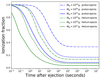Fig. 2. Time evolution of the ionization fraction of the ejecta. Different line styles represent cases of different ejecta mass, while different colors represent different composition. Recombination effect is important and generally the heavier the ejecta, the lower the ionization fraction. For pure helium ejecta, the ionization fractions are much lower than those of hydrogen ejecta, giving rise to smaller DM and RM contributions.

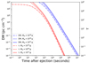Fig. 3. Time evolution of the DM and τff contributed by a typical hydrogen ejecta.

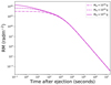Fig. 4. Time evolution of the RM contributed by a typical ejecta.

Apart from M_ej, there are many more parameters that can have a impact on the RM evolution. The influence of B₀ is quite straightforward. The spin period determines the light cylinder radius; therefore, this will also influence RM according to Eq. (10). The choice of v_max,  v_min influences the decay timescale of RM and DM. The time needed for the contribution becomes negligible is shorter for ejecta moving out with higher speed. Furthermore, the initial temperature of the ejecta will influence the recombination rate, thus indirectly influence the RM values. This is shown in Fig. 5 that the higher initial temperature, the more abundant free electrons and the greater RM.

Fig. 5. Similar to Fig. 4, but fixing Mej = 1021 g and allowing T0 vary.

4. Applications to two special FRB events

In this section, I discuss the application of our model to two special FRBs. The rapid change of RM is a natural outcome of matter ejection according to above section. I assumed the magnetar flare occurs at T_start (in MJD). Taking (M_ej,  B₀,  P₀,  T_start) as the parameters and fixing s = −1,  v_min = 0.0001c,  v_max = 0.1c,  T₀ = 10⁸ K, I used a Markov chain Monte Carlo (MCMC) approach and found the RM data can be well fitted, as shown in Fig. 6a. At the same time, the τ_ff and DM contributed by the ejecta are both negligible (see Fig. 6b). Outside the period of the abrupt RM change phase, there are stochastic fluctuations of RM and DM with mean values of $\overline{\mathrm{RM}}=21.2$ rad m⁻², $\overline{\mathrm{DM}}=249.4$ pc cm⁻³, which are adopted as their baseline values respectively. The pink and cyan area in Figure 6 show the long-term variation ranges with respect to the baseline values. The best-fitting parameters are listed in Table 1 and the relevant corner plot is shown in Fig. A.1. All parameters are contained within a reasonable range and, therefore, the magnetar flare scenario is fitting to explain this special RM behavior.

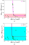Fig. 6. Fitting results of FRB 20220529 by the flare scenario. (a): Model fitting of the RM behavior. A baseline value $\overline{\mathrm{RM}}=21.2$ rad m−2 has been subtracted. The shaded pink region shows the RM variation range outside the abrupt RM change period. (b): Time evolution of DM and τff under the best-fitting parameters in Table 1. The DM contribution by the ejecta is very small, compared to the stochastic fluctuation shown by the shaded cyan area.

Different from FRB 20220529, no significant RM change was observed for the Galactic FRB 20200428D, which should also be explained within this scenario. As I discuss above, the amplitude and the decay timescale of RM depend on several parameters. For the source magnetar SGR 1935+2154, the spin period is P₀ = 3.245 s and magnetic field strength is B₀ ≃ 2.2 × 10¹⁴ G. Both values have been determined from observations (Israel et al. 2016). Therefore, we can adjust other parameters to reduce the RM contribution. As an example, I fixed M_ej = 10²¹ g, T₀ = 10⁶ K, s = −2, v_max = 0.3c, and let v_min vary. A relative large v_max was adopted for this magnetar to ensure that the total kinetic energy of flare ejecta matched its observed X-ray burst energy of ∼10³⁹ erg. The result is shown in Fig. 7. Just after ∼10⁴ s, both RM and DM fall below unity. If we do not have the good fortune to catch an FRB within such a short timescale after the flare, the signal of RM contribution by the ejecta would probably be missed in observations. This is likely the case for FRB 20200428D, since it is not a very active repeater. There is an X-ray burst accompanying FRB 20200428D, which might indicate matter ejection. However, a detailed analysis suggested that the radio burst occurred slightly earlier than X-ray burst; therefore, these ejected shells will have no influence on DM and RM.

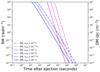Fig. 7. Possible set of parameters explaining the absence of notable RM change for FRB 20200428D. Both RM and DM contribution decline to unity rapidly, therefore, they can hardly be identified in observations.

5. Discussion and conclusions

In this work, I have constructed a simple toy model for the structure of magnetar flare ejecta and calculated its possible contribution to RM and DM values of FRBs. I find that for canonical magnetar flare parameters, it is possible to identify the RM change from observations. It is certainly more difficult to identify the DM change because after the time of τ_ff <  1, the DM contribution by the ejecta is only moderate (≲10 pc cm⁻³) and decays rapidly. I note that there is a suitable “time window” to identify these variational behaviors in observations. Below ∼0.1 days, the ejecta is still opaque due to free-free absorption, whereas above a few tens of days, the RM contribution from the ejecta becomes negligible. Assuming that the magnetar flare ejection (X-ray activity) and FRB production are physically unrelated, it is easier for an active repeater to have a burst falling in this time window. In this sense, it is a natural expectation that this RM change was observed for FRB 20220529, but not for FRB 20200428D due to a difference in source activity. Moreover, the relevant parameters of FRB 20220529 source magnetar may be more preferred to give rise to RM change. Therefore, as long as FRB 20220529 maintains its activity, similar sudden RM changes are guaranteed to be discovered by long-time monitoring of this source.

In this work, I adopted the simplest case that the ejecta is spherically symmetric and the viewing angle θ = 0. In principle, the angular structure could be more complicated. Due to the limited number of bursts with RM measurements in flare stage, the angular structure cannot be constrained well and performing a model fitting based on the simple case is good enough. If we have the ability to observe another similar case with adequate datapoints characterizing the RM evolution in great detail, probing the structure of ejecta will be realizable in the future. One critical advantage of our model is that the magnetar itself can complete the process without a companion; therefore, the occurrence rate of a similar RM change is higher than that of binary model. The probability of a companion ejecting coronal mass at right time and the right direction is very low.

As there are specific opportunities to observe sudden RM change contributed by the flare ejecta, I encourage the search for FRBs following X-ray bursts of magnetars within a time lag of ∼10⁵ s. In particular, SGR 1935+2154 has a relatively high activity in X-rays, but it only emits FRBs occasionally. The redshift of FRB 20220529 source is a bit high (z = 0.1839); thus, the X-ray flux is too low to be detected by current X-ray satellites when assuming typical burst luminosity of ∼10⁴¹ erg. Therefore, we can scarcely forecast when a similar sudden RM change will occur without an X-ray notice. We look forward to the possibility of witnessing an active repeating FRB associated with enormous X-ray activity in the future, which will allow us to test our model in detail and help break the parameter degeneracy.

Acknowledgments

I am grateful to an anonymous referee for helpful comments. This work is supported by the National Natural Science Foundation of China (Grant Nos. 12373052, 12321003, 12393813) and the National SKA Program of China (2022SKA0130100).

References

Appendix A: Parameter corner plot of the MCMC results

Fig. A.1. Parameter corner plot of the MCMC results. The contours are 1σ, 2σ, and 3σ uncertainties.

All Tables

All Figures

	Fig. 1. Schematic picture of the toy model. The ejecta are composed of several ion shells with different velocities. The mass distribution is not necessarily uniform for both the radial and angular directions.
In the text

Fig. 2. Time evolution of the ionization fraction of the ejecta. Different line styles represent cases of different ejecta mass, while different colors represent different composition. Recombination effect is important and generally the heavier the ejecta, the lower the ionization fraction. For pure helium ejecta, the ionization fractions are much lower than those of hydrogen ejecta, giving rise to smaller DM and RM contributions.

In the text

	Fig. 3. Time evolution of the DM and τff contributed by a typical hydrogen ejecta.
In the text

	Fig. 4. Time evolution of the RM contributed by a typical ejecta.
In the text

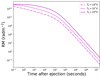	Fig. 5. Similar to Fig. 4, but fixing Mej = 1021 g and allowing T0 vary.
In the text

Fig. 6. Fitting results of FRB 20220529 by the flare scenario. (a): Model fitting of the RM behavior. A baseline value $\overline{\mathrm{RM}}=21.2$ rad m−2 has been subtracted. The shaded pink region shows the RM variation range outside the abrupt RM change period. (b): Time evolution of DM and τff under the best-fitting parameters in Table 1. The DM contribution by the ejecta is very small, compared to the stochastic fluctuation shown by the shaded cyan area.

In the text

	Fig. 7. Possible set of parameters explaining the absence of notable RM change for FRB 20200428D. Both RM and DM contribution decline to unity rapidly, therefore, they can hardly be identified in observations.
In the text

	Fig. A.1. Parameter corner plot of the MCMC results. The contours are 1σ, 2σ, and 3σ uncertainties.
In the text

References

- Anna-Thomas, R., Connor, L., Dai, S., et al. 2023, Science, 380, 599 [NASA ADS] [CrossRef] [Google Scholar]
- Bochenek, C. D., Ravi, V., Belov, K. V., et al. 2020, Nature, 587, 59 [NASA ADS] [CrossRef] [Google Scholar]
- Bogovalov, S. V. 1999, A&A, 349, 1017 [Google Scholar]
- Burbidge, G. R., Gould, R. J., & Pottasch, S. R. 1963, ApJ, 138, 945 [Google Scholar]
- CHIME/FRB Collaboration (Andersen, B. \^{A}. C., et al.) 2020, Nature, 587, 54 [NASA ADS] [CrossRef] [Google Scholar]
- Gelfand, J. D., Lyubarsky, Y. E., Eichler, D., et al. 2005, ApJ, 634, L89 [NASA ADS] [CrossRef] [Google Scholar]
- Huang, Z.-Q., Liu, L.-D., Wang, X.-Y., & Dai, Z.-G. 2018, ApJ, 867, 6 [Google Scholar]
- Israel, G. L., Esposito, P., Rea, N., et al. 2016, MNRAS, 457, 3448 [NASA ADS] [CrossRef] [Google Scholar]
- Kalapotharakos, C., & Contopoulos, I. 2009, A&A, 496, 495 [NASA ADS] [CrossRef] [EDP Sciences] [Google Scholar]
- Kaneko, Y., Göḡü, E., Baring, M. G., et al. 2021, ApJ, 916, L7 [Google Scholar]
- Kaspi, V. M., & Beloborodov, A. M. 2017, ARA&A, 55, 261 [Google Scholar]
- Li, C. K., Lin, L., Xiong, S. L., et al. 2021, Nat. Astron., 5, 378 [NASA ADS] [CrossRef] [Google Scholar]
- Li, Y., Zhang, S. B., Yang, Y. P., et al. 2025, ArXiv e-prints [arXiv:2503.04727] [Google Scholar]
- Lorimer, D. R., Bailes, M., McLaughlin, M. A., Narkevic, D. J., & Crawford, F. 2007, Science, 318, 777 [Google Scholar]
- Lyutikov, M. 2003, MNRAS, 346, 540 [Google Scholar]
- Margalit, B., & Metzger, B. D. 2018, ApJ, 868, L4 [NASA ADS] [CrossRef] [Google Scholar]
- Mereghetti, S., Savchenko, V., Ferrigno, C., et al. 2020, ApJ, 898, L29 [Google Scholar]
- Mestel, L. 1973, Ap&SS, 24, 289 [Google Scholar]
- Michel, F. C. 1973a, ApJ, 180, 207 [Google Scholar]
- Michel, F. C. 1973b, ApJ, 180, L133 [Google Scholar]
- Okamoto, I. 1974, MNRAS, 167, 457 [Google Scholar]
- Petroff, E., Hessels, J. W. T., & Lorimer, D. R. 2022, A&ARv, 30, 2 [NASA ADS] [CrossRef] [Google Scholar]
- Philippov, A. A., Spitkovsky, A., & Cerutti, B. 2015, ApJ, 801, L19 [NASA ADS] [CrossRef] [Google Scholar]
- Ridnaia, A., Svinkin, D., Frederiks, D., et al. 2021, Nat. Astron., 5, 372 [NASA ADS] [CrossRef] [Google Scholar]
- Spitkovsky, A. 2006, ApJ, 648, L51 [Google Scholar]
- Tavani, M., Casentini, C., Ursi, A., et al. 2021, Nat. Astron., 5, 401 [NASA ADS] [CrossRef] [Google Scholar]
- Thompson, C., & Duncan, R. C. 1995, MNRAS, 275, 255 [Google Scholar]
- Tucker, W. H., & Gould, R. J. 1966, ApJ, 144, 244 [Google Scholar]
- Wang, F. Y., Zhang, G. Q., Dai, Z. G., & Cheng, K. S. 2022, Nat. Commun., 13, 4382 [NASA ADS] [CrossRef] [Google Scholar]
- Xiao, D., Wang, F., & Dai, Z. 2021, Sci. China Phys. Mech. Astron., 64, 249501 [NASA ADS] [CrossRef] [Google Scholar]
- Xu, H., Niu, J. R., Chen, P., et al. 2022, Nature, 609, 685 [NASA ADS] [CrossRef] [Google Scholar]
- Yang, Y.-P., & Zhang, B. 2017, ApJ, 847, 22 [Google Scholar]
- Yang, Y.-P., Xu, S., & Zhang, B. 2023, MNRAS, 520, 2039 [NASA ADS] [CrossRef] [Google Scholar]
- Younes, G., Güver, T., Kouveliotou, C., et al. 2020, ApJ, 904, L21 [CrossRef] [Google Scholar]
- Zhang, B. 2023, Rev. Mod. Phys., 95, 035005 [NASA ADS] [CrossRef] [Google Scholar]
- Zhao, Z. Y., Zhang, G. Q., Wang, F. Y., & Dai, Z. G. 2023, ApJ, 942, 102 [NASA ADS] [CrossRef] [Google Scholar]
- Zhu, W., Xu, H., Zhou, D., et al. 2023, Sci. Adv., 9, eadf6198 [NASA ADS] [CrossRef] [Google Scholar]