| Issue |
A&A
Volume 690, October 2024
|
|
|---|---|---|
| Article Number | A300 | |
| Number of page(s) | 21 | |
| Section | Extragalactic astronomy | |
| DOI | https://doi.org/10.1051/0004-6361/202450825 | |
| Published online | 17 October 2024 | |
Virgo Filaments
III. The gas content of galaxies in filaments as predicted by the GAEA semi-analytic model
1
Dipartimento di Fisica e Astronomia Galileo Galilei, Università degli studi di Padova, Vicolo dell’Osservatorio, 3, I-35122 Padova, Italy
2
INAF – Osservatorio astronomico di Padova, Vicolo dell’Osservatorio, 5, I-35122 Padova, Italy
3
INAF – Osservatorio Astronomico di Trieste, Via Tiepolo 11, I-34131 Trieste, Italy
4
IFPU - Institute for Fundamental Physics of the Universe, via Beirut 2, 34151 Trieste, Italy
5
Siena College, 515 Loudon Rd., Loudonville, NY 12211, USA
6
The University of Kansas, Department of Physics and Astronomy, Malott Room 1082, 1251 Wescoe Hall Drive, Lawrence KS 66045, USA,
7
Observatoire de Paris, LERMA, Collège de France, CNRS, PSL University, Sorbonne University, 75014 Paris, France
8
INAF – Osservatorio di Astrofisica e Scienza dello Spazio di Bologna, via Gobetti 93/3, I-40129 Bologna, Italy
9
Laboratoire d’astrophysique, Ecole Polytechnique Fédérale de Lausanne (EPFL), Observatoire, CH-1290 Versoix, Switzerland
10
Tianjin Normal University, Binshuixidao 393, 300387 Tianjin, China
11
Institute for Physics, Laboratory for Galaxy Evolution and Spectral modelling, Ecole Polytechnique Federale de Lausanne, Observatoire de Sauverny, Chemin Pegasi 51, 1290 Versoix, Switzerland
Received:
22
May
2024
Accepted:
6
August
2024
Abstract
Galaxy evolution depends on the environment in which galaxies are located. The various physical processes (ram-pressure stripping, tidal interactions, etc.) that are able to affect the gas content in galaxies have different efficiencies in different environments. In this work, we examine the gas (atomic HI and molecular H2) content of local galaxies inside and outside clusters, groups, and filaments as well as in isolation using a combination of observational and simulated data. We exploited a catalogue of galaxies in the Virgo cluster (including the surrounding filaments and groups) and compared the data against the predictions of the Galaxy Evolution and Assembly (GAEA) semi-analytic model, which has explicit prescriptions for partitioning the cold gas content in its atomic and molecular phases. We extracted from the model both a mock catalogue that mimics the observational biases and one not tailored to observations in order to study the impact of observational limits on the results and predict trends in regimes not covered by the current observations. The observations and simulated data show that galaxies within filaments exhibit intermediate cold gas content between galaxies in clusters and in isolation. The amount of HI is typically more sensitive to the environment than H2 and low-mass galaxies (log10[M⋆/M⊙]< 10) are typically more affected than their massive (log10[M⋆/M⊙]> 10) counterparts. Considering only model data, we identified two distinct populations among filament galaxies present in similar proportions: those simultaneously lying in groups and isolated galaxies. The former has properties more similar to cluster and group galaxies, and the latter is more similar to those of field galaxies. We therefore did not detect the strong effects of filaments themselves on the gas content of galaxies, and we ascribe the results to the presence of groups in filaments.
Key words: galaxies: clusters: general / galaxies: evolution / galaxies: clusters: individual: Virgo / large-scale structure of Universe
Corresponding author; This email address is being protected from spambots. You need JavaScript enabled to view it.
© The Authors 2024
 Open Access article, published by EDP Sciences, under the terms of the Creative Commons Attribution License (https://creativecommons.org/licenses/by/4.0), which permits unrestricted use, distribution, and reproduction in any medium, provided the original work is properly cited.
This article is published in open access under the Subscribe to Open model. This email address is being protected from spambots. You need JavaScript enabled to view it. to support open access publication.
1. Introduction
In recent years, studies on the influence of the environment have established that the properties of galaxies correlate with their local density. Galaxies in clusters typically have earlier morphological types (Dressler 1980; Vulcani et al. 2023), are more massive, (Kauffmann et al. 2004; Baldry et al. 2006), have reduced star formation (Peng et al. 2010; Woo et al. 2013; Vulcani et al. 2010; Paccagnella et al. 2016; Finn et al. 2023), and contain less cold gas (Giovanelli & Haynes 1985; Brown et al. 2017) than galaxies in lower density regions (Rojas et al. 2004; Beygu et al. 2016).
While the most striking differences are found when comparing galaxies in the field and in clusters, it has become clear that ‘intermediate’ environments, such as groups and filaments, also play an important role. Nevertheless, determining the environment of a galaxy poses a challenge. For instance, there is no obvious separation between clusters and groups, as they can be considered as elements of the large-scale structure (LSS) gathering into filaments and walls (Bond et al. 1996). Secondly, filament identification is challenged by a number of observational effects (e.g. the fingers-of-god effect due to the peculiar velocities of galaxies) that distort the actual distribution of galaxies (Kuchner et al. 2021), which in turn affects filament extraction. Equally important, the identification of filaments depends on the tracer: Zakharova et al. (2023) have shown that galaxies of different mass trace the underlying distribution of dark matter differently.
Despite the difficulties related to the determination of the galaxy environments, it has been found that galaxies within filaments exhibit notable differences from their cluster and field counterparts. Independent studies consistently indicate that filament galaxies tend to be more massive (Laigle et al. 2017; Malavasi et al. 2017; Zakharova et al. 2023) and redder (Kuutma et al. 2017; Kraljic et al. 2017; Singh et al. 2020) and to have lower star-formation rates (SFRs; Kraljic et al. 2017; Sarron et al. 2019) than galaxies in the field. Some studies have found evidence of a distinct impact of filaments on different gas phases. Vulcani et al. (2019) found that in some filament galaxies, ionised Hα clouds extend far beyond what is seen for other non-cluster galaxies. This result may be due to the effective cooling of the dense star-forming regions in filament galaxies, which can increase the spatial extent of the Hα emission. Also, atomic HI and molecular gas reservoirs have been shown to be impacted by the filament environment (Kleiner et al. 2017; Crone Odekon et al. 2018; Blue Bird et al. 2020; Lee et al. 2021; Castignani et al. 2022a).
The effect of filament environment on galaxy properties remains debated because filaments contain groups of various masses (Tempel et al. 2014) that may contribute to the measured differences of the properties of filament members with respect to those of galaxies in the field (Sarron et al. 2019).
The trends observed for galaxies in dense regions can be explained by the impact of mechanisms characteristic of dense environments, such as ram-pressure stripping of gas (Gunn et al. 1972; Bahé et al. 2017), tidal effects (Bekki 1998), galaxy-galaxy interactions (Naab et al. 2007), and mergers (Mihos & Hernquist 1996; Kaviraj et al. 2009). These processes typically affect the gas content of galaxies since they can displace and remove it, resulting in the suppression of star formation (De Lucia et al. 2012; Wetzel et al. 2012). All of the mechanisms listed above affect the gas content of galaxies. Therefore, a strong correlation is expected between the amount of gas in galaxies and their environment.
The nearby massive Virgo cluster and its surrounding filaments are an ideal laboratory for comparing the properties of galaxies in various environments. The first work of this series, (Castignani et al. 2022a), focused on gathering and analysing data about the gas content of galaxies around the Virgo cluster. The authors of that work collected both atomic and molecular gas content information for galaxies within the cluster (from Boselli et al. 2014) and filaments in an extended region around the cluster by using both new observations and existing data in the literature. Data were compared with isolated galaxies from the AMIGA survey (Verdes-Montenegro et al. 2005), and the results showed a decreasing gas content moving from the field to filaments and then clusters as well as an increase of the proportion of quiescent galaxies. Castignani et al. (2022a) concluded that the processes leading to the suppression of star formation in galaxy clusters are already starting to take place in filaments.
The second paper of this series, (Castignani et al. 2022b), compiled an exceptional dataset for ∼7000 galaxies around the Virgo cluster into a catalogue (based on the Kim et al. 2014 catalogue), combining spectroscopically confirmed sources across multiple databases and surveys, such as HyperLeda, NASA Sloan Atlas, NED, and ALFALFA. The resulting catalogue provides positions, masses, integrated HI and CO, and a parametrisation of the environment for galaxies surrounding Virgo. In addition, Castignani et al. (2022b) conducted an analysis of galaxy properties within Virgo filaments, confirming that filament members indeed have intermediate properties (local density, galaxy morphology, bar fractions) between galaxies in the cluster and the field.
This paper is the third of the series, and it is dedicated to examining two main points. First, we wanted to test whether current state-of-the-art semi-analytical models can reproduce the observed gas properties of galaxies across different environments. Second, we wished to investigate how the gas content of galaxies around the Virgo cluster depends on the environment. In particular, our aim is to understand the role of filaments in regulating the gas content of galaxies from a theoretical point of view. To do so, we took advantage of a state-of-the-art theoretical model of galaxy formation, GAEA. Unlike widely used hydrodynamical models such as IllustrisTNG (Nelson et al. 2018; Springel et al. 2018; Pillepich et al. 2018; Naiman et al. 2018; Marinacci et al. 2018), EAGLE (Schaye et al. 2015), and The Three Hundred project (Cui et al. 2018) or constrained simulations such as Simulating the LOcal Web (SLOW; Dolag et al. 2023; Hernández-Martínez et al. 2024; Böss et al. 2023) and HESTIA (Libeskind et al. 2020), GAEA includes an explicit treatment for the partition of cold gas in its atomic and molecular components, and it is coupled to a large cosmological volume with relatively high resolution.
The paper is organised as follows. Section 2 describes the observational and model samples used in this work. In Sect. 3, we parametrize the environment for each observed and model galaxy. In Sect. 4, we describe how we constructed our model mock sample to be compared with data. Section 5 compares the gas properties of galaxies in the cluster, filaments, and field both for the observational sample and the mock data. In Sect. 6, we discuss the role of filaments in regulating the gas content in the Virgo cluster surroundings. Section 7 summarises the results of this paper.
2. Data description
2.1. Observational data
We made use of the Virgo Filament catalogue, which was released in Castignani et al. (2022b). The catalogue is based on data from different databases and surveys, including HyperLeda, NASA Sloan Atlas, and NASA/IPAC Extragalactic Database, and contains information about 6780 galaxies within ∼12 virial radii around the Virgo cluster. The catalogue covers the region delimited by 100° < RA < 280° and −1.3° < Dec < 75°, and contains galaxies with recessional velocities 500 < vr < 3300 km/s. It also includes 110 galaxies that have recessional velocities < 500 km/s but have redshift-independent distances in the NASA/IPAC Extragalactic Database (NED-D; Steer et al. 2017) that correspond to cosmological velocities in the range of 500–3300 km/s. Some of these galaxies are Virgo cluster members that are located near the caustics, and thus have the largest deviations in velocity from Virgo. More details on the catalogue construction and on how it was cleaned from spurious sources, stars, and duplicates can be found in Castignani et al. (2022b).
We estimated the stellar masses and SFRs from spectral energy distribution (SED) fitting. We construct the SEDs from publicly available, wide-area imaging surveys that span from the UV to the infrared. Specifically, we use: FUV and NUV from GALEX (Gil de Paz et al. 2007); grz imaging from the DESI Legacy Imaging Surveys (DESI Collaboration 2016); and 3.4μ, 4.5μ, 12μ and 22μ from WISE Wright et al. (2010). Magnitudes in each photometric band are determined from a custom elliptical aperture photometry pipeline that is optimised for large, nearby galaxies. The photometry and masking methods are based on those developed for the Siena Galaxy Atlas and are described in detail in Moustakas et al. (2023). Our fluxes are measured within a fixed elliptical aperture whose semi-major axis is 1.5 times the estimated size of the galaxy based on the second moment of the light distribution (after subtracting stars and masking out surrounding galaxies in the image). We do not attempt to correct the aperture fluxes to total fluxes. However, using a curve-of-growth analysis, we estimate that the correction would affect the stellar masses by < 20%. To correct for galactic extinction, we use the redenning values from Schlegel et al. (1998) and follow the Legacy Survey’s procedure to transform to the grz and WISE filters. We transform E(B − V) to extinction in the GALEX FUV and NUV filters using the transformations in Wyder et al. (2007).
We used the Multi-wavelength Analysis of Galaxy Physical Properties (MAGPHYS) tool (da Cunha et al. 2008) to model the SEDs and estimate stellar masses and SFRs (rely on the Chabrier 2003 initial mass function). Following the Legacy Survey, we use the gz filters for galaxies with Declination δ > 32.375 and the grz filters for galaxies south of this limit. This difference in the inclusion of the z-band is because there are known offsets in the relative z-band calibration in the northern survey that are more pronounced for galaxies with larger angular extent. We verified using the southern filters that removing the z-band did not affect our SED-fitting results. The southern filters were already incorporated into MAGPHYS, and the northern filters were added to the MAGPHYS package following a request to its creator (Da Cunha, priv. comm.).
We determined the stellar mass completeness limit, above which we will detect all galaxies regardless of their r-band stellar mass-to-light ratio (M⋆/Lr). We derived the stellar mass completeness limit using a technique adapted from Marchesini et al. (2009), Rudnick et al. (2017), and Finn et al. (2023). We started with galaxies at the high velocity (distance) end of our survey, namely those with 2500 < v/km/s < 3500 as these will have the faintest observed brightness at a fixed mass or luminosity. We selected all galaxies between 0.5 and 1.25 mag brighter than the SDSS spectroscopic limit of mr = 17.77. These galaxies are bright enough that we should be able to detect all galaxies with equal completeness, regardless of their M⋆/Lr. We make the reasonable assumption that M⋆/Lr does not vary strongly with observed magnitude over this range. Therefore, the distribution of M⋆/Lr for this bright subsample should be consistent with the intrinsic M⋆/Lr distribution near our apparent magnitude limit. Using this distribution of M⋆/Lr, we measure the 5% highest M⋆/Lr. At the luminosity limit of our survey, corresponding to the apparent magnitude limit of the most distant galaxies, this M⋆/Lr limit yields a stellar mass limit of log(M⋆/M⊙) = 8.26. Galaxies at lower stellar masses would only be detectable if they had lower M⋆/Lr values.
From here on, we use only galaxies with the measured stellar masses above the mass completeness limit of the catalogue (log[M⋆/M⊙]> 8.3), for a total of 2919 galaxies. We used this sample to identify filaments (see Sect. 3).
For part of the Castignani et al. (2022b) sample, HI and H2 observations were obtained in Castignani et al. (2022a). They presented a compilation of the available data: the catalogue contains information about atomic (MHI) and molecular hydrogen (MH2) for galaxies with stellar masses 9 < log10(M⋆/M⊙) < 11. Specifically, data are available for 389 galaxies of which 97 are cluster galaxies, 166 filament galaxies1, and 132 are galaxies in the field. Briefly, Castignani et al. (2022a) collected HI observations for the Virgo cluster galaxies from Boselli et al. (2014). For the galaxies in the longest filaments with the highest contrast around Virgo, they collected data from the literature and observed the missing galaxies with the Nançay telescope (59 galaxies in the catalogue). HI masses for field galaxies were also taken from the literature (mainly Verdes-Montenegro et al. 2005; Springob et al. 2005). 82 galaxies with HI measurements had molecular hydrogen measurements from the literature, while the rest were observed with the IRAM-30 m (both CO(1 → 0) and CO(2 → 1), simultaneously). A detailed description of these data and how HI and H2 masses were estimated can be found in Castignani et al. (2022a).
2.2. Simulated data
We used predictions from the GAlaxy Evolution and Assembly (GAEA) semi-analytic model (Hirschmann et al. 2016) coupled with the Millennium II Simulation (Boylan-Kolchin et al. 2009). GAEA2 builds on the original model presented in De Lucia & Blaizot (2007), but it includes a number of important updates. In particular, we use here the latest rendition of the model presented in De Lucia et al. (2024), that includes: (i) a detailed treatment for the non-instantaneous recycling of gas, metals, and energy that allows different elemental abundances to be traced explicitly (De Lucia et al. 2014; ii) an updated treatment for stellar-feedback that provides good agreement with the observed evolution of the galaxy stellar mass function up to z ∼ 3 and other important scaling relations (Hirschmann et al. 2016); (iii) an explicit treatment for partitioning the cold gas in its atomic and molecular components, and for ram-pressure stripping of both the hot gas and cold gas reservoirs of satellite galaxies (Xie et al. 2017, 2020); (iv) an updated treatment of AGN feedback that includes an improved modelling of cold gas accretion on supermassive black holes and an explicit implementation for quasar winds (Fontanot et al. 2021). De Lucia et al. (2024) have shown that the latest renditions of GAEA provides an improved agreement with the observed distributions of specific SFRs in the local Universe, as well as a quite good agreement with the observed passive fractions up to z ∼ 3, making this model version an ideal tool to interpret the data considered in this work. The results of the model are based on the Chabrier IMF Chabrier (2003).
We took advantage of a GAEA realisation run on dark matter halo merger trees extracted from the Millennium II simulation, which followed 21603 dark matter particles in a box of 100 Mpc h−1 on a side, with cosmological parameters consistent with WMAP1 (ΩΛ = 0.75, Ωm = 0.25, Ωb = 0.045, n = 1, σ8 = 0.9, and H0 = 73 km s−1 Mpc−1). The high resolution of the simulation (the particle mass is  ) allows galaxies to be well resolved down to stellar masses of 108 M⊙.
For our analysis, we used the following information for each model galaxy: 3D positions and velocities, the mass of the hosting dark matter halo (M200, mass of the region enclosing a mean density of 200ρcrit, where ρcrit is critical density of the Universe), stellar mass, mass of HI and of H2, galaxy type (central or satellite), and star formation rate.
The model includes an explicit treatment of the interaction of satellite galaxies with the host halo gas (both stripping of the hot gas associated with satellites and ram-pressure stripping of cold gas). A detailed description of that can be found in Xie et al. (2020). Being coupled with merger trees extracted from N-body simulations, it also accounts for assembly bias – that is, earlier assembled haloes are more clustered than later assemblies of similar mass (Gao et al. 2005), which leads to an impact on galaxies properties (Croton et al. 2007; Wang et al. 2013). We emphasize that the GAEA model does not include any explicit mechanism accounting for the interaction of galaxies with filaments.
For comparison with the observations, we extract from GAEA all halos having a mass similar to that of Virgo ( Kourkchi & Tully 2017) at z ∼ 0. Only three such halos exist in the Millennium II volume, and their virial masses are
  (GAEA V1),
  (GAEA V2) and
  (GAEA V3).
2.2.1. GAEA coordinate transformation
The first step of our analysis is to extract from the model simulated box portions of the sky of a size comparable to the one covered by the observations. The catalogue by Castignani et al. (2022b) is based on a RA-Dec-vr selection within a fixed area around Virgo. We obtain the same coordinates for each galaxy in GAEA: first of all, we position the simulated volume at the same distance of the Virgo cluster (∼16 Mpc/h, Mei et al. 2007) and select galaxies in a range of radial velocities vr relative to the cluster centre similar to that of the observational sample. Next, we transform the GAEA cartesian coordinates x-y-z in RA-Dec-vr to be able to cut the same region in RA-Dec-vr coordinates. We also obtain supergalactic coordinates SGX-SGY-SGZ, which we use to identify filaments. This procedure is detailed in Appendix A.
As a final step, we select a region similar to the one analysed by Castignani et al. (2022b) around the Virgo cluster and consider only galaxies with 100° < RA < 280° and −1.3° < Dec < 75° and have matching velocities 500 < vr < 3300 km/s. Since some of the Virgo cluster members have vr < 500 km/s (see Castignani et al. 2022b for more details), then we do not apply this condition for cluster members (galaxies inside 3 virial radii of the cluster centre, regardless of their vr). We hence obtain three regions of the sky around three Virgo-like systems (GAEA V1, GAEA V2, and GAEA V3). We note that our cubes include distortions in the distribution of galaxies associated with line-of-sight effects (as do the observational data). We do not make any adjustments to these effects to be consistent with the previous works in the series.
2.2.2. Stellar mass completeness limit and the selection function
Next, we apply the same mass cut estimated for the observations (logM⋆/M⊙ > 8.3). At this stage, the number of galaxies in each of the three GAEA regions is on average 3–5 times higher than the sample of Castignani et al. (2022b) above the same mass completeness cut. As discussed above, the Virgo Filament catalogue is a combination of different datasets and, as such, it is characterised by a selection function that is hard to precisely replicate (Castignani et al. 2022b). Instead of trying to emulate the ‘incompleteness’ for each of the three regions, we reduce the number of galaxies by performing one random extraction of a sample that has the same number of galaxies found in the observed sample (2518) and a similar stellar mass distribution.
Figure 1 shows the result of the extraction of three Virgo-like regions and the observations in the RA-Dec plane.
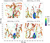 |
Fig. 1. Distribution of galaxies around the Virgo cluster (top-left panel, from Castignani et al. 2022b) and around the three Virgo-like clusters in the GAEA model (top right: GAEA V1, bottom left: GAEA V2, bottom right: GAEA V3) in celestial coordinates (corresponding to the GAEA-all sets; Sect. 4.1). The label of each panel indicates the mass of Virgo or of the Virgo-like halos. Each point is a galaxy with |

3. Environmental definitions
3.1. Identification of filaments
To identify filaments, Castignani et al. (2022b) exploited a tomographic approach to characterize the highest density contrasts relative to the surrounding field as determined by visual inspection. Briefly, they considered the eight filamentary structures presented in Tully (1982) and Kim et al. (2016), and visually identified 5 additional filaments. For each filament, they considered an associated cuboid in the 3D supergalactic frame large enough to enclose all galaxies that belong to the structure under consideration. They then determined the filament spines by fitting the locations of the galaxies in supergalactic coordinates. The method developed by Castignani et al. (2022b) requires visual inspection, which makes it very difficult to replicate. Therefore, we opt for a redefinition of the filamentary structure based on the Discrete Persistent Structures Extractor (DisPerSE, Sousbie 2011; Sousbie et al. 2011) code. In this way, we can rely on a consistent definition between the observational and simulated samples. We refer to the original papers for detailed information on the algorithm employed by DisPerSE. Briefly, using information about the distribution of galaxies, the code estimates a density distribution that is then used to identify the spines of the filamentary structure. Different ‘persistence’ levels can be chosen to identify filaments with different contrast. The higher the persistence level, the higher the density of the detected filaments: for instance, a threshold of 7σ finds only the densest structures, while a threshold of 3σ finds many more short filaments (length less than a typical cluster radius), many of which might correspond to spurious detections (see Zakharova et al. 2023 for more details).
We tested using DisPerSE on the observational sample and we recover approximately the same structures identified by Castignani et al. (2022b), although with different levels of details. Using the supergalactic coordinates SGX-SGY-SGZ, we extracted filaments from the observed sample adopting different persistence levels (3σ, 4σ, 5σ, and 7σ) to identify filaments characterised by different density contrasts.
At the 3σ threshold, the DisPerSE-defined filaments system (FS) catches almost all the structures defined by Castignani et al. (2022b) but also a number of additional filaments. Adopting this persistence level, up to 70% of the galaxies turn out to be in filaments. This values is too large when compared to the catalogue by Castignani et al. (2022b). In addition, many of the identified filaments are extremely faint. In contrast, the FS obtained using a persistence level of 5σ or larger loses some of the filaments identified by Castignani et al. (2022b), including some very dense ones. As a compromise, we choose a 4σ persistence level. With this threshold, we find that the visual approach and DisPerSe would give consistent result. We have verified that the adoption of a new method to determine the filaments has no impact on the scientific results obtained with the approach by Castignani et al. (2022b).
We apply the 4σ persistence level for the extraction of filaments using DisPerSE both for observations and for the simulated regions. In both cases, we also remove all filaments that are shorter than 3 Mpc/h (of the order of 7 ± 3 filaments depending on the analysed sample), as it is hard to establish if they are real structures. As noted above, the simulated regions GAEA V1, GAEA V2, and GAEA V3 described in Sect. 2.2.1 include the fingers-of-god effect (the elongation along the line-of-sight). This also affects filament identification, as we discuss in detail in Appendix B. Briefly, elongation along line-of-sight does not greatly interfere with the classification of galaxies as members in filaments, but it also does not allow one to determine the exact distance to the axis of the filaments.
Following Castignani et al. (2022b), in both the model and observations, we consider a galaxy to be in a filament if its distance to the nearest filament segment is less than 2 Mpc/h and if the galaxy does not belong to the cluster (see the cluster membership definition below). We exclude from the filaments the cluster members as we expect that the effect of the cluster environment is dominant over the possible effect of the filaments (Sarron et al. 2019; Kraljic et al. 2017). Figure 1 also highlights in red the members of the selected filaments for the three extracted clusters and the observed data.
3.2. Additional environments around Virgo
In addition to the filaments, Castignani et al. (2022b) considered other environments in the region around the Virgo cluster. First of all, they identified cluster members, selecting galaxies within 3.6 Mpc/h from the Virgo cluster centre in the 3D SG coordinate frame. The chosen radius corresponds approximately to ∼3R200. They also considered as cluster members those galaxies that fall within the cluster region delimited by the caustics in the phase-space diagram, regardless of their SG coordinates. Then, they identified galaxy groups by matching their catalogue to the environmental catalogue from Kourkchi & Tully (2017), who characterised galaxy groups in our immediate neighbourhood (vr < 3500 km/s). Finally, they assembled a sample of pure field galaxies, that is, galaxies that do not belong to the cluster nor to a filament or a group.
Here, we adopt an approach similar to that of Castignani et al. (2022b). For the observations, we use their exact definition for cluster and group galaxies, while we redefine the pure field sample by using the same method but considering our definition of filament members.
To identify these same environments for GAEA galaxies, we proceed as follows. For each simulated region (GAEA V1, GAEA V2, and GAEA V3), we define as cluster members those galaxies with a clustercentric distance < 3R200 Mpc/h in 3D. As mentioned above, we exclude these galaxies when defining filament membership. To identify groups, we do not consider the true halo memberships provided by the model as this membership definition would be very different from the observational one, based on a compilation of available observations with different depths. In an attempt to reproduce the observations, we select from the GAEA samples V1, V2, and V3 all halos that have at least one galaxy member in our samples. We then computed the number of galaxies in each of these halos. We defined a group as any gravitationally bounded structure with more than one galaxy log[M⋆/M⊙]> 8.3. Given that this approach to select groups is still different from the observed one, we avoided considering a finer division in groups based on their richness and simply separated isolated galaxies from aggregations of any size.
Finally, we defined pure field galaxies as those galaxies not belonging to any filaments nor to any group or cluster.
We checked if pure field galaxies are actually members of filaments with a density contrast lower than that of the adopted persistence level. However, only 10% of the pure field galaxies are members of the filaments identified using a 3σ persistence level.
4. Galaxy samples in observations and GAEA
In the previous sections we have introduced the analysed samples and provided a characterisation of the environments we are going to consider in this work. In this section we finalize the galaxy samples we will use, and introduce some definitions useful for the analysis presented below.
4.1. Observational gas mass limit
As mentioned in Sect. 2.1, measurements of atomic and/or molecular hydrogen are not available for all galaxies in the catalogue by Castignani et al. (2022b): some of them have simply not been observed, while for some others only upper limits have been obtained, given their low gas content. The limit down to which the gas mass could be obtained for all galaxies depends on many parameters: in terms of fluxes, it depends on the integration time and telescope sensitivity, but in terms of masses, it also depends on full width at half maximum (FWHM) of the detected signal, distance of the source, the observed CO transition, the gas excitation, and aperture correction. To perform a meaningful comparison between observational and simulated data, it is important to mimic the observed gas mass completeness of the catalogue, separately for the HI and H2 masses. Given the nature of the observations gathered by Castignani et al. (2022a), who collected literature data in addition to their own campaigns, it is not possible to properly determine the completeness limits. We, therefore, manually select the HI and H2 levels above which we consider GAEA and observational samples as complete. Figure 2 separately shows the HI and H2 masses as a function of stellar mass for observations and the thresholds we adopt as completeness limit. The separation was obtained as the line that best separates actual measurements from upper limits:
![Mathematical equation: $$ \begin{aligned} \log [\mathrm{M}_{\mathrm{HI}}/ \mathrm{M}_{\odot }]&> -0.5 \cdot \log [\mathrm{M}_{\star }/ \mathrm{M}_{\odot }] + 12.7,\end{aligned} $$](/articles/aa/full_html/2024/10/aa50825-24/aa50825-24-eq7.gif) (1)
(1)
![Mathematical equation: $$ \begin{aligned} \log [\mathrm{M}_{{\mathrm{H}_{2}}}/ \mathrm{M}_{\odot }]&> -0.15 \cdot \log [\mathrm{M}_{\star }/ \mathrm{M}_{\odot }] + 9.0. \end{aligned} $$](/articles/aa/full_html/2024/10/aa50825-24/aa50825-24-eq8.gif) (2)
(2)
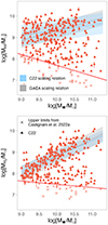 |
Fig. 2. The scaling relation between MHI (top) and MH2 (bottom) as a function of stellar mass for observations. Red triangles show measurements, and crosses show upper limits. The solid red line shows the adopted level of completeness limits of the observations for HI (Eq. (1)) and H2 (Eq. (2)) masses, respectively. Shaded areas show the scaling relations for C22 (light blue, Eq. (3) in the top panel, Eq. (4) in the bottom panel) and for GAEA (light grey, Eq. (5) in the top panel, Eq. (6) in the bottom panel). |
We additionally checked that changing this level does not affect the results of this paper.
From now on, in both observations and in the model, we will use only the galaxies with MHI or MH2 above the separation lines in Fig. 2, and with stellar masses in the range  . We will conduct all the analysis on the HI (H2) content considering only the galaxies above the MHI (MH2) level, regardless of the H2 (HI) content. When both the HI and H2 will be considered simultaneously, we will use only the galaxies with both MHI and MH2 above the corresponding levels.
Finally, since the stellar mass distribution of the observed galaxies could have an impact on the results, considering each environment separately, we randomly extract from the model samples with the same stellar mass distribution as that of the observed sample. Specifically, we randomly select the same stellar mass distribution 100 times for each environment in the GAEA V1, GAEA V2, and GAEA V3 cubes. We will call the GAEA sample with this adopted gas limit and stellar mass distribution ‘GAEA-mock’. We will call the observed sample drawn from Castignani et al. (2022b) as explained in the previous section’s ‘C22 sample’.
In addition to the GAEA-mock, we will also consider the GAEA sample relaxing the cut in gas mass, and we will call it ‘GAEA-all’. This sample also includes only galaxies with stellar masses  . It will be used to study the impact of observational limits on the results and predict trends in regimes not covered by the current observations. We summarize all the performed steps for each of these sets in Fig. 3. The number of galaxies in the different samples is given in Tables 1 and 2.
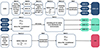 |
Fig. 3. Schematic view of the steps needed to obtain the final sample for both the model (GAEA-all, GAEA-mock) and the observed sample (C22). Each step is described in the main text (Sects. 2, 3, 4). |
Number of galaxies with HI measurements above the gas mass completeness limit in C22, GAEA-mock, and all in each environment separately. The model data provides the median number of samples among the three halos under consideration.
4.2. Definition of gas deficiency
A common way to investigate the effect of the environment on the gas content of galaxies is to measure the gas deficiency (e.g. Giovanelli & Haynes 1985; Haynes 1985; Haynes & Giovanelli 1986; Casoli et al. 1998; Chung et al. 2009; Boselli et al. 2014; Hess et al. 2015; Healy et al. 2021; Moretti et al. 2023), which is defined as the difference between the gas content of a galaxy belonging to a given environment and that of a field galaxy of the same size and morphology.
The exact definition of HI and H2 deficiency varies from study to study and depends on the specifics of the observational sample (e.g. available information). In this work, we base HI and H2 deficiencies on the gas mass versus stellar mass relation.
In this section, we obtain the HI and H2 scaling relations needed to obtain the HI and H2 deficiency parameters (HIdef and H2, def, respectively) separately in the observations and in the model. The main sequences (MS) MHI − M⋆ calculated for the model and data separately helped us not to have to worry about how well the model reproduces the observational MS (although we show below that they are close to each other).
In observations, we separately define scaling relations for HI and H2 using the sample described in Sect. 4.1. As we aim at obtaining a general scaling relation, here we use only star-forming (specific star formation rate sSFR > 10−11 year−1) field galaxies ( , with Mhalo mass of group as derived by Kourkchi & Tully 2017 from the Ks-band luminosity by using M/L ratios), regardless of their filament membership. By fitting the data using a linear regression method, we obtained the following scaling relations:
![Mathematical equation: $$ \begin{aligned} \log [\mathrm{M}_{\mathrm{HI}}/ \mathrm{M}_{\odot }]&= 0.25 \cdot \log [\mathrm{M}_{\star } / \mathrm{M}_{\odot }] + 6.82 \pm 0.49,\end{aligned} $$](/articles/aa/full_html/2024/10/aa50825-24/aa50825-24-eq12.gif) (3)
(3)
![Mathematical equation: $$ \begin{aligned} \log [\mathrm{M}_{{\mathrm{H}_{2}}}/ \mathrm{M}_{\odot }]&= 0.8 \cdot \log [\mathrm{M}_{\star } / \mathrm{M}_{\odot }] + 0.76 \pm 0.35. \end{aligned} $$](/articles/aa/full_html/2024/10/aa50825-24/aa50825-24-eq13.gif) (4)
(4)
Figure 2 shows these relations on the top and bottom panels, with a light-blue area marking 1-sigma scatter, respectively.
In GAEA, we defined the scaling relations using all the field galaxies in the full cube. As in observations, we considered only star-forming galaxies (sSFR > 10−11 year−1) that are not part of structures with a halo mass  above the gas mass completeness limits (Fig. 2). As before, we fit the data using a linear regression method and obtained the following scaling relations:
![Mathematical equation: $$ \begin{aligned} \log [\mathrm{M}_{\mathrm{HI}}/ \mathrm{M}_{\odot }]&= 0.47 \cdot \log [\mathrm{M}_{\star } / \mathrm{M}_{\odot }] + 4.67 \pm 0.34,\end{aligned} $$](/articles/aa/full_html/2024/10/aa50825-24/aa50825-24-eq15.gif) (5)
(5)
![Mathematical equation: $$ \begin{aligned} \log [\mathrm{M}_{{\mathrm{H}_{2}}} / \mathrm{M}_{\odot }]&= 0.71 \cdot \log [\mathrm{M}_{\star }/\mathrm{M}_{\odot }] + 1.7 \pm 0.26. \end{aligned} $$](/articles/aa/full_html/2024/10/aa50825-24/aa50825-24-eq16.gif) (6)
(6)
These relations are also shown in Fig. 2 by light-grey areas and are in excellent agreement with the observational determination.
We were then in the position of defining the HI and H2 deficiencies as the logarithmic difference between the expected (for a given mass) and measured HI and H2 mass, respectively:
![Mathematical equation: $$ \begin{aligned} {\mathrm{HI}}_{\mathrm{def}}&= \log [\mathrm{M}_{\mathrm{HI}}^{ \mathrm{EXP}}/ \mathrm{M}_{\odot }] - \log [\mathrm{M}_{\mathrm{HI}}^{ \mathrm{MES}}/ \mathrm{M}_{\odot }],\end{aligned} $$](/articles/aa/full_html/2024/10/aa50825-24/aa50825-24-eq17.gif) (7)
(7)
![Mathematical equation: $$ \begin{aligned} {\mathrm{H}}_{2,\mathrm{def}}&= \log [\mathrm{M}_{{\mathrm{H}_{2}}}^{ \mathrm{EXP}}/ \mathrm{M}_{\odot }] - \log [\mathrm{M}_{{\mathrm{H}_{2}}}^{ \mathrm{MES}}/ \mathrm{M}_{\odot }], \end{aligned} $$](/articles/aa/full_html/2024/10/aa50825-24/aa50825-24-eq18.gif) (8)
(8)
with ![Mathematical equation: $ \log[\mathrm{M}_{\mathrm{HI}}^{ \mathrm{EXP}}/ \mathrm{M}_{{\odot}}] $](/articles/aa/full_html/2024/10/aa50825-24/aa50825-24-eq19.gif) obtained from Eq. (3) for observations and Eq. (5) for GAEA,
obtained from Eq. (3) for observations and Eq. (5) for GAEA, ![Mathematical equation: $ \log[\mathrm{M}_{{\mathrm{H}_{2}}}^{ \mathrm{EXP}}/ \mathrm{M}_{{\odot}}] $](/articles/aa/full_html/2024/10/aa50825-24/aa50825-24-eq20.gif) obtained from Eq. (4) for observations, and Eq. (6) for GAEA.
obtained from Eq. (4) for observations, and Eq. (6) for GAEA.
In this work, we consider a galaxy as HI (H2) deficient when HIdef > 0.5 (H2, def > 0.5), and we consider HI (H2) normal if HIdef ≤ 0.5 (H2, def ≤ 0.5).
We note that Castignani et al. (2022a) adopted a different definition of deficiency, which involves only field galaxies within the same morphological type and optical sizes. Here, we do not adopt their approach to be consistent in definitions between the observations and the model However, we compare the deficiency values used by Castignani et al. (2022a) and ours, finding a good correlation (see Appendix C). A more thorough discussion on the different ways to define the expected MHI or MH2 to estimate deficiencies can be found in Li et al. (2020) or Cortese et al. (2021) and is beyond the scope of this work.
5. Results: HI and H2 content
In this section we characterize the gas content of galaxies in cluster, filaments and pure field using both the observed data and the model predictions. We first consider the atomic hydrogen content and investigate how galaxies are distributed on the MHI − M⋆ plane and discuss how the HI-deficiency distributions depend on the position of galaxies within the cosmic web. Next, we repeat the same analysis for the molecular hydrogen H2 content. Finally, we combine the two measurements and contrast HI and H2 deficiency and look for correlations.
5.1. Atomic hydrogen HI content
In this section we use only galaxies with MHI above the limit given in Eq. (1), both for C22 and GAEA-mock samples, regardless of their H2-content.
The top panel of Fig. 4 shows the relation between MHI and stellar mass M⋆ for galaxies in different environments for C22, GAEA-mock, and GAEA-all. In agreement with the vast literature (e.g. Catinella et al. 2010; Parkash et al. 2018), we recover a positive correlation between MHI and M⋆. Overall, the C22 and GAEA-mock galaxy samples, which by construction are directly comparable, occupy the same region of the plane. Furthermore, while most of the galaxies are concentrated around the scaling relation defined by Eq. (5), a non-negligible population deviates from it, having a lower MHI than expected, given their stellar mass. The fraction of cluster galaxies with reduced MHI is comparable between C22 and GAEA-mock samples and is 49 ± 7% and 51 ± 6%, respectively. Similarly, also the relative abundance of pure field galaxies with low levels of MHI are compatible: in both cases they are 17 ± 5%. Filament galaxies have intermediate position in terms of reduced amounts of atomic hydrogen in 43 ± 5% cases for C22 and 41 ± 5% for GAEA-mock.
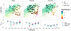 |
Fig. 4. The amount of HI-content in galaxies in clusters, filaments, and pure field. Top: MHI as a function of stellar mass in different environments, indicated on top of each panel. The GAEA model data are shown with circles: small circles represent the GAEA-all set, and big circles represent one of the 300 realisations of the GAEA-mock sample. Big triangles show the C22 data. In all the samples, each point is coloured by sSFR. In each panel, the solid grey line shows the MHI − M⋆ scaling relation (Eq. (5)), the dotted line shows the 0.5 dex indent to highlight HI-deficiency zone. The faint red line represents HI-mass completeness limit from Eq. (1). Bottom: Fractions of HI-deficient galaxies (see Sect. 4.2) with 1σ confidence interval as a function of stellar mass. |
Our results are qualitatively consistent with many previous works that found an increased proportion of galaxies with reduced MHI in clusters compared to field galaxies of similar mass (Haynes 1985; Boselli & Gavazzi 2006) and that filament galaxies occupy an intermediate position between cluster and field galaxies (e.g. Blue Bird et al. 2020; Castignani et al. 2022a). In addition, we note that the model does reproduce observational data for galaxies in filaments, although the model does not include a special treatment for filaments.
When considering GAEA-all, we find that the fraction of low HI-content galaxies decreases from clusters (74 ± 1%) to filaments (57 ± 2%) to pure field (32 ± 1%). However, the absolute numbers are higher than for C22 and GAEA-mock, which is obviously due to the adopted gas mass limit in Sect. 4.1.
The bottom panel of Fig. 4 shows how the fraction of HI-deficient galaxies depends on stellar mass, where median fractions of HIdef with 1σ confidence interval for each mass bin are reported. C22 and GAEA-mock provide a consistent picture: overall, where there is enough statistics, the HI-deficient galaxy fraction increases with increasing stellar mass, except in the observed Virgo cluster where it is consistent with being flat across the considered mass range. The GAEA-all sample, which allowed us to get rid of some observational biases, shows instead different trends. In the cluster and in filaments, the fraction of HI-deficient galaxies decreases with increasing stellar mass. This result is due to the fact that in GAEA low-mass galaxies are more affected by ram-pressure stripping forces because of their low restoring force Gunn et al. (1972). As a consequence, they have a higher probability of being HI-deficient (see also Xie et al. 2020).
The points in the top panel of Fig. 4 are coloured by the galaxy sSFR. In general, in both the GAEA-mock and C22 samples galaxies with relatively low MHI are also characterised by low sSFR values. This is particularly true for high-mass galaxies. There are though some exceptions, with galaxies with normal HI gas content having already low sSFR values (in agreement with e.g. Zhang et al. 2019) and, vice-versa, galaxies with reduced MHI but with high sSFR values, indicative of non-negligible, ongoing star formation. However, this is not unexpected: star formation is found to be more strongly correlated with the surface density of molecular hydrogen than with atomic hydrogen (Leroy et al. 2008).
The results presented above rely on the adopted separation between HI-normal and HI-deficient galaxies. To obtain more general results, in Fig. 5 we consider the distribution of the HI-deficiency, and investigate how the whole population of galaxies behaves in the different environments. To account for the dependence on stellar mass in Fig. 4, we then consider two mass bins: low-mass (log10[M⋆/M⊙]< 10) and massive (log10[M⋆/M⊙]> 10) galaxies.
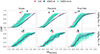 |
Fig. 5. HI-deficiency cumulative distribution function for GAEA-all (three lines for GAEA-all V1, GAEA-all V2 and GAEA-all V3); GAEA-mock (300 lines); and C22 split into the different environments and two mass bins (low-mass log10[M⋆/M⊙]< 10 and massive galaxies log10[M⋆/M⊙]> 10). In each plot, the median values with a 1σ confidential interval are reported. The grey vertical line shows the 0.5 HI-deficiency level as a level adopted to consider a galaxy as HI-deficient. |
Overall, the cumulative distribution function of the HI-deficiency in the GAEA-mock is compatible to that obtained for C22, in each environment and in both mass bins. Considering the low-mass galaxies, C22 and GAEA-mock retrieve consistent trends: 43 ± 8% and 52 ± 10% of the cluster population have a HI-deficiency parameter > 0.5 dex. Moving to filaments and pure field, the median values of the distributions shift to lower values, indicating galaxies are most likely HI-normal (only 29 ± 6% (13 ± 7%) and 30 ± 6% (17 ± 9%) of low-mass filaments (pure field) galaxies are HI-deficient for C22 and GAEA-mock, respectively). We additionally confirm the correspondence between C22 and GAEA-mock low-mass galaxies in terms of HI-deficiency running the KS test pairwise on C22 and each of the 300 realisations of the GAEA-mock sample. Considering each environment separately, we find that distributions are indistinguishable (p-v > 0.05) in at least 90% of the cases for cluster and filaments samples, and only in 77% for pure field.
The comparison between GAEA-all and C22/GAEA-mock in Fig. 5 shows how the adopted gas mass limit affects the completeness of the low-mass galaxy population. GAEA-all predicts a much more substantial fraction of HI-deficient low-mass galaxies in cluster (76 ± 1%), in filaments (61 ± 2%), and in pure field (30 ± 1%) than observed.
The case of massive galaxies is similar to the low-mass one: the fraction of HI-deficient galaxies is the greatest for cluster members (C22 shows 61 ± 8%, GAEA-mock have 52 ± 9% HI-deficient massive galaxies) and declines to filaments (56 ± 6% for C22 and 44 ± 7% for GAEA-mock) and pure field (16 ± 8% for C22 and 25 ± 11% for GAEA-mock) although clusters and filaments fractions are compatible within errors. Figure 5 shows a correspondence between the cumulative distribution functions of HI-deficiency of massive galaxies in C22 and GAEA-mock within each environment. We confirm this result with the KS test, which reports that distributions are indistinguishable (p-v > 0.05) in 99%, 87%, and 97% of the cases for cluster, filaments, and pure field galaxies, respectively. Due to the adopted gas mass completeness limit, we do not observe any significant difference between GAEA-all and C22/GAEA-mock for massive galaxies. Overall, GAEA-all predicts 62 ± 6%, 54 ± 5%, and 32 ± 4% of HI-deficient massive galaxies in clusters, filaments, and pure fields, respectively.
To summarize, we find an excellent agreement between the C22 and GAEA-mock samples and also detect for all three sets a decrease in the proportion of HI-deficient galaxies from clusters to filaments and to the pure field. However, we do not find a significant difference between massive and low-mass galaxies in C22/GAEA-mock in cluster and pure field, although GAEA-all predicts that the proportion of HI-deficient low-mass galaxies is higher than the proportion of massive ones within cluster and filaments.
5.2. Molecular hydrogen H2
Next, we focus on the H2 content of galaxies. For C22 and GAEA-mock, we used only galaxies with MH2 above the limit Eq. (2),3 regardless of their HI-content.
The top panel of Fig. 6 shows the mass of molecular hydrogen MH2 as a function of stellar mass for galaxies in different environments for GAEA and C22. As in the case of MHI, we recover a correlation between MH2 − M⋆ for all the considered environments and a good agreement between C22 and GAEA-mock samples. A significant H2-deficient population in cluster and filaments emerges. In GAEA-mock, the fraction of H2-deficient galaxies (H2, def > 0.5) decreases from cluster (38 ± 7%) to filaments (26 ± 4%) and pure field (14 ± 4%) galaxies. Similarly, C22 shows the fraction of H2-deficient galaxies is 29 ± 7% in the cluster, 26 ± 4% in the filaments, and 13 ± 5% in the pure field. The bottom panel of Fig. 6 shows the fraction of H2-deficient galaxies in different environments and mass bins. GAEA-mock and C22 provide consistent results within errors for each of the environments: the fraction of H2-deficient galaxies rapidly increases with increasing stellar mass. At the same time, GAEA-all predicts an U-like shape in the fraction of H2-deficient galaxies, where galaxies with log10[M⋆/M⊙]< 9 or log10[M⋆/M⊙]> 10.5 have a higher probability of being H2-deficient.
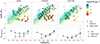 |
Fig. 6. The amount of H2-content in galaxies in clusters, filaments, and pure field. Top: MH2 as a function of stellar mass in the different environments. Panels, colours, and symbols are as in Fig. 4. Bottom: Fractions of H2-deficient galaxies in each environment by mass bins. Panels, colours, and symbols are as in Fig. 4. |
The correspondence between the GAEA-mock and C22 for the molecular hydrogen allowed us to make predictions according to GAEA-all for the fraction of H2-deficient galaxies without observational biases: 65 ± 2% of cluster galaxies 51 ± 2% of filament galaxies and 25 ± 1% of the pure filament galaxies are H2-deficient. We note that the fractions of H2-deficient galaxies are lower than those of HI-deficient galaxies, in each environment separately (by ≈10% for cluster and filaments and by ≈5% for pure field). This is most likely due to the fact that by design GAEA includes the removal of HI ahead of H2, to match observational results (see Boselli et al. 2014 or Cortese et al. 2021 for a review).
Points in Fig. 6 (left panel) are colour-coded by sSFR values. As expected, H2-deficient galaxies are also quiescent, in all environments (Leroy et al. 2008). Nevertheless, in C22 20% of cluster galaxies with normal H2 content are quiescent, while GAEA does not predict the existence of this population.
Figure 7 shows the cumulative distribution function of H2-deficiency for galaxies in various environments in two mass bins for GAEA-all, GAEA-mock, and C22. According to GAEA-mock, clusters have a higher fraction of low-mass (log10[M⋆/M⊙]< 10) H2-deficient galaxies than filaments and pure field: 28 ± 9%, 12 ± 4% and 4 ± 4%, respectively. This is in broad agreement with the C22 sample where fractions are 16 ± 6%, 13 ± 4%, and 8 ± 4% for low-mass galaxies in the same environments. Overall, these values are significantly lower than those obtained for the HI-deficiency, both in observations and in the model, indicating that HI must be removed more rapidly than H2, in all environments and regardless of the mechanisms affecting the gas content.
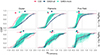 |
Fig. 7. H2-deficiency distributions (CDF) and median values with 1σ confidential interval. The caption is the same as Fig. 5. The number of samples is presented in Table. 2. |
To further check the correspondence between the GAEA-mock and C22 for low-mass galaxies, we run the KS test between the different distributions. The KS test reveals that GAEA-mock does not reproduce C22 H2-deficiency properly for cluster and pure field: only 6% and 30% of GAEA-mock samples have indistinguishable distributions from observed ones. In contrast, when comparing distributions in filaments, we retrieve no difference between the model and C22 in 98% of the GAEA-mock realisations.
Considering massive galaxies (log10[M⋆/M⊙]> 10), we obtain the following fractions of H2-deficient galaxies for C22 and GAEA-mock respectively: 44 ± 12% and 44 ± 9% for cluster galaxies ; 46 ± 9% and 41 ± 8% for filament galaxies, and 25 ± 13% and 22 ± 12% for pure field galaxies. Thus, massive galaxies have a similar fraction of H2-deficiency in all the environments. Also, C22 (but not GAEA-mock) shows the same values for low-mass ones in filaments and the cluster.
The KS test between C22 and GAEA-mock for massive galaxies shows a good correspondence for H2-deficiency distribution in 69%, 86%, and 88% for the cluster, filaments, and pure field galaxies. Considering the GAEA-all sets, we obtain a similar trend of decreasing fraction of H2-deficient galaxies from the cluster to filaments and to the pure field for low-mass (67 ± 1%, 52 ± 1% and 23 ± 1%, respectively) and massive galaxies (56 ± 4%, 52 ± 4% and 38 ± 6%, respectively).
Taking into account observational biases, we conclude that the GAEA model is reproducing how the H2-deficiency depends on the environment, especially for massive galaxies.
5.3. HI- vs H2-deficiency
Having established that similar H2-deficiency and HI-deficiency trends are found in GAEA-mock and C22, we then combine the HI-deficiency and H2-deficiency measurements. Figure 8 shows the H2, def–HIdef relation for galaxies in different environments and within two stellar mass bins, considering only galaxies with both HI and H2 masses above the corresponding thresholds 4 (Eqs. (1) and (2)). Each panel shows the separation between HI-deficient/H2-deficient and HI-normal/H2-normal regions, so each panel is separated into four quadrants: I (HI- and H2-normal galaxies), II (HI-normal and H2-deficient galaxies), III (HI- and H2-deficient galaxies), IV (HI-deficient and H2-normal galaxies).
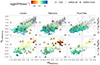 |
Fig. 8. H2, deficiency–HIdeficiency relations for low-mass (top) and massive (bottom) galaxies in clusters (left), filaments (middle), and the pure field (right). GAEA-mock data is represented by big circles, GAEA-all data by small circles, and C22 data by triangles. Each point of the GAEA-mock/C22 is coloured by sSFR. The vertical and horizontal lines show 0.5 dex deficiency levels used to separate gas normal from gas deficient galaxies. |
For all samples, Fig. 8 shows a clear correlation between H2, def and HIdef for each environment and mass bins, in agreement with other works (e.g. Zabel et al. 2022; Moretti et al. 2023). The proportion of galaxies with deficiency only in one gas phase according to GAEA-all does not exceed 20% across all environments and mass bins (17 ± 1% for low-mass galaxies and 15 ± 3% for massive ones). The GAEA-all sample, plotted in the background, highlights the already discussed observational biases emerging for low-mass and HI- and H2-deficient (III quadrants) galaxies: GAEA-all predicts a population of low-mass HI- and H2-deficient galaxies, which are under the gas mass completeness limits. Comparing C22 and GAEA-mock, we find that low-mass galaxies are mostly located in the first quadrant. Moreover, low-mass galaxies are star-forming regardless of the surroundings, either for C22 or GAEA-mock: more than 90% if galaxies in each environment separately have sSFR > 10−11 year−1.
The top panels of Fig. 8 also show how HI and H2-deficiency for low-mass galaxies depends on the environment according to GAEA-all: the fractions of galaxies inside III quadrant decline from cluster to filaments and pure field: 62 ± 2%, 45 ± 1% and 16 ± 1%, respectively. The third quadrant contains mostly galaxies with low sSFR (70% of III quadrant galaxies are quiescent with sSFR < 10−11 year−1), which is expected since the absence of cold gas is inevitably connected to suppressed star formation in galaxies (Leroy et al. 2008; Boselli et al. 2014).
Among massive galaxies, C22 and GAEA-mock mostly occupy the first and the third quadrants, as well as GAEA-all. However, GAEA-all predicts a smaller difference in fractions of HI and H2-deficient galaxies between environments for massive galaxies (as was discussed above) than for low-mass systems: 48 ± 5%, 49 ± 1% and 26 ± 4 for the cluster, filaments, and pure field. GAEA-mock follows this trend with 33 ± 9% of the cluster, 33 ± 8% filaments, and 17 ± 9% pure field galaxies inside the III quadrant. C22 sample shows 24 ± 9%, 39 ± 8%, and 17 ± 9% of HI- and H2-deficient in cluster, filaments, and field. We stress that here we are considering only galaxies above both HI and H2 thresholds and we are therefore using a subsample of that used in the previous section. This is the reason why results seems at odds with what previously shown.
In Sect. 5.2 we discussed the presence of H2-normal galaxies but without ongoing star formation. Figure 8 reveals that those galaxies are strongly HI-deficient galaxies. It is surprising since we do not expect that HI-deficiency is sufficient to prevent star formation in galaxies with normal H2.
To summarize the entire section, when considering as much as possible the several observational biases, and the inability to accurately reproduce the selection function, the model reproduces the HI content in galaxies for each of the three considered environments when separated into low-mass and massive galaxies. The replication by the model of H2 content in filaments and in the pure field as well is good, but for cluster galaxies, we obtained uncertainty in H2-deficiency, which is apparently related to observational biases. Finally, we show that the difference in the proportion of HI and/or H2-deficiency of low-mass galaxies across all the environments is more pronounced than for massive galaxies. So, massive galaxies are less sensitive to environments than low-mass galaxies either for HI- and H2-deficiency. In addition, both the model and observations show that the difference in HI-deficiency between environments is more pronounced than H2-deficiency, suggesting that HI is more sensitive to the environment, in agreement with previous works (Boselli et al. 2014; Loni et al. 2021).
6. Discussion
In the previous section we have shown that results obtained using the GAEA model and observations are in broad agreement; we discuss the influence of filaments on the evolution of galaxies using only the GAEA-all dataset, which is not affected by observational biases. We will examine how filaments influence galaxy evolution in terms of assembly history (at fixed halo mass, the assembly of dark matter haloes correlates with the large-scale environment Gao et al. 2005, which in turn is imprinted on the assembly of galaxies Croton et al. 2007). We again emphasize that the GAEA model does not include any specific treatment for galaxies in filaments other than assembly bias. This means that there is no predetermined dependence of galaxy properties on the distance to the axis of the filaments, galaxy-filament interaction is not considered and there are no specific modes of accretion of cold gas to galaxies in filaments. Instead, the GAEA model includes the assembly bias in dense surroundings and the interaction with host halos for satellite galaxies (De Lucia et al. 2024).
As schematically illustrated in Fig. 9, filaments can contain both galaxy groups and isolated galaxies (alone in their halo). In GAEA-all, which includes galaxies with  , 51 ± 1% of the filament members are simultaneously group members (17 ± 1%, 18 ± 1% and 14 ± 1% for 1 < Nmem < 5, 5 < Nmem < 15, 15 < Nmem groups, respectively), while 49 ± 1%5 of the total filament population are galaxies in isolation – from now on “pure filament galaxies”6. None of the two populations are negligible. These results were obtained taking into account the selection function, so the fraction of pure filament galaxies was overestimated. Indeed, Kuchner et al. (2022) reported only 33% of pure filament galaxies (pristine in their nomenclature).
We are now in the position of better characterising the role of filaments in galaxy evolution: (i) considering galaxies in both groups and filaments, we can investigate whether the presence of groups in the filaments plays a relevant role and, at a fixed mass of the group, whether members of groups outside and inside the filaments have the same HI or H2 content (Sect. 6.1); (ii) considering only pure filament galaxies we can investigate the influence of filaments on the evolution of galaxies, excluding any group contributions (Sect. 6.2). Indeed, in GAEA, pure filament galaxies are, by construction, treated similarly to pure field galaxies (single galaxies inside their haloes). According to our definition of galaxy environment, the only distinction between pure field and pure filament galaxies is their distance from the filaments, with the former being more than 2 Mpc/h away from a filament axis and the latter being closer.
6.1. Dependence on halo mass
We investigate whether the filaments have an impact on the galaxies within haloes of fixed mass. To do this, we compare the deficiency of atomic and molecular hydrogen in halos of equal mass inside and outside the filaments. In order to avoid any biases related to the fact that massive haloes are more prevalent inside filaments while low-mass haloes are more dominant outside filaments (Welker et al. 2018), we first fit the Mhalo distribution for haloes inside and outside filaments.
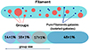 |
Fig. 9. Schematic representation of filament composition by galaxies in groups of different sizes and pure filament galaxies (i.e. alone in their halo; top panel). The proportion of galaxies in groups with 15 < Nmem < 50, 5 < Nmem < 15, and 1 < Nmem < 5 members and pure filament in total filaments population, respectively (bottom panel), taking into account the selection function. |
Figure 10 shows the HI-deficiency and H2-deficiency as a function of the host halo mass Mhalo for GAEA-all separately for galaxies inside and outside filaments. The figure presents the median value with 1σ significance interval for the galaxies inside and outside filaments within Mhalo bins.
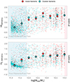 |
Fig. 10. The dependency of atomic and molecular content at fixed halo mass for galaxies inside and outside filaments. Top: HI-deficiency as a function of the host halo mass Mhalo in GAEA-all. Colour coding reflects the position concerning filaments: inside or outside. Big circles show median values with 1σ confidential interval for galaxies inside and outside filaments in each mass bin (median values were estimated for similar Mhalo distribution for haloes inside and outside filaments by bootstrapping). On the background, typical pure filament/pure field (90%-quantile) and clusters of halo masses are highlighted. Bottom: Same but for H2-deficiency. |
Overall, the median HI-deficiency and H2-deficiency monotonously increase with the increasing host halo mass. The median HI- or H2-deficiency for a given Mhalo is the same within errors for galaxies inside and outside filaments. Thus, galaxies inside groups with  , either inside and outside filaments, have the same HI and H2-deficiency; that is, the location of the group inside or outside the filaments does not have a significant effect on the amount of cold gas in galaxies. Thus, we do not detect a difference between the deficit of atomic and molecular hydrogen in satellites in groups (the proportion of central galaxies in the considered halos
  is 3 %) inside and outside the filaments, but we note that Poudel et al. (2017) detects a difference between the central galaxies.
Figure 10 also allowed us to directly compare galaxies inside and outside the filaments (which we classified as pure filament and pure fields, respectively). Since up to 90% of isolated galaxies are located within low-mass haloes  , these objects populate the light blue/grey shaded area in Fig. 10. For both HI- and H2-deficiency, at fixed halo mass isolated galaxies inside and outside filaments have a comparable deficiency of atomic or molecular hydrogen. Therefore, we do not detect any signs of the role of filaments on HI- or H2-content for pure filament members.
6.2. The impact of filaments on the galaxy HI and H2 content
The most common method for determining the influence of filaments on galaxies is to check the dependence of their properties (mass/star formation rate/amount of gas) as a function of the distance to the filaments (e.g., Singh et al. 2020; Hasan et al. 2024. Observations have shown that the influence of filaments on galaxy properties is usually more pronounced near the filaments axis: galaxy in filaments are typically redder (Singh et al. 2020), more HI-deficient (Crone Odekon et al. 2018; Lee et al. 2021), more massive (Kraljic et al. 2017) and have earlier morphological types (Castignani et al. 2022a) if they lie closer the filament axis.
Following the same approach, for each galaxy from GAEA-all, we determine the 3D distance to its nearest filament. Next, we define the HI- and H2-deficiency as a function of distance to filament for galaxies in groups, filaments, pure filament, and pure field separately. Results are presented in Fig. 11. In agreement with previous works (Castignani et al. 2022a; Crone Odekon et al. 2018; Lee et al. 2021; Hoosain et al. 2024), filament members close to the filament axis are more HI- and H2-deficient that in the outer parts of the filaments (top panels): HIdef = 0.96 ± 0.17 and H2, def = 0.66 ± 0.2 at Dfil < 0.5 Mpc/h vs HIdef = 0.48 ± 0.07 and H2, def = 0.33 ± 0.06 at 1.5 < Dfil < 2.0 Mpc/h. In contrast, pure filament galaxies show much lower absolute values of both HI- and H2-deficiency (HIdef = 0.35 ± 0.5 and H2, def = 0.17 ± 0.2 at Dfil < 0.5 Mpc/h) and almost no dependence on the distance to filament. Moreover, pure field galaxies shows the same properties of HI- and H2-deficiency as pure filament galaxies. This emphasizes that these galaxies essentially have similar properties of atomic and molecular hydrogen.
 |
Fig. 11. HI- or H2-deficiency (median values and 1σ significance interval) as a function of 3D distance to the nearest filament in GAEA-all for filaments, the pure filament, and pure fields (top panels), and members of groups of different sizes: 1 < Nmem < 5, 5 < Nmem < 15, 15 < Nmem< 50 (bottom panels). |
The right panels of Fig. 11 consider members of groups of different sizes: 1 
 , and
, and  507. Galaxies in groups closer than 2 Mpc/h from the filaments axis are also members of the filaments. Overall, group galaxies inside and outdside filaments are more HI- and H2-deficient than pure filament galaxies, regardless of the group richness. 1 < Nmem < 5 groups statistically show lower HI- and H2-deficiencies than bigger groups (5 < Nmem < 15, and 15 < Nmem < 50) and do not show a dependence on the proximity to filaments. In contrast, groups with 5 < Nmem < 15 and 15 < Nmem < 50 show a higher HI- and H2-deficiency close to the filament axis: HIdef = 1.36 ± 0.74 and H2, def = 1.23 ± 0.85 at Dfil < 0.5 Mpc/h vs HIdef = 1.07 ± 0.16 and H2, def = 0.72 ± 0.11 at 1.5 < Dfil < 2.0 Mpc/h in groups 5 < Nmem < 15 (HIdef = 1.06 ± 0.4 and H2, def = 0.85 ± 0.35 at Dfil < 0.5 Mpc/h vs HIdef = 1.01 ± 0.3 and H2, def = 0.7 ± 0.12 at 1.5 < Dfil < 2.0 Mpc/h in groups 15 < Nmem < 50). We note that all the dependencies given in this section are calculated relative to filaments, taking into account peculiar velocity distortions (see Appendix B for the details). We discuss the impact of the line-of-sights distortions on the filament extraction on this test in Appendix D.
As a consequence, the result of filament galaxies having gas content intermediate between the cluster and the pure field, shown in Sect. 5 and in Castignani et al. (2022a), can be explained by the fact that filaments host both galaxies in groups, and pure filament galaxies, in similar proportions and that the two populations have different HI and H2 properties.
Besides, Hoosain et al. (2024) found in the RESOLVE survey (Stark et al. 2016) and the ECO catalogue (Eckert et al. 2017) that compared group galaxies and isolated systems inside filaments, they also reveal that tendency of overall filaments members to be more HI and H2-deficient (i.e. intermediate properties) near the filament axis relate to the increasing roles of galaxy groups inside filaments rather than isolated galaxies (isolated galaxies close do not demonstrate dependency of HI and H2-deficiency on the distance to filaments).
Our statement that galaxies in pure filament have similar properties to galaxies in the pure field is based mainly on the fact that the dependence of the HI- and H2-deficiency does not depend on the distance to the filaments. However, our filament structure was calculated taking into account elongation along line-of-sight effects, which did not allow us to accurately estimate the distance to the filament axis (see Appendix B) and can consequently distort the results of this test. Therefore, we repeat the same exercise, after having redefined the environment and distance to filaments for each galaxy from GAEA-all relative to the ‘true filaments‘. We call ‘true filaments‘ those determined by DiSPerSE using the distribution of all galaxies with log10[M⋆/M⊙]> 8.3 in the cartesian coordinates x-y-z of the model around Virgo-like clusters with a persistence level of 4σ (as described in Appendix B). We also consider as pure filament galaxies only those who are truly isolated in the model; that is, there are no other gravitationally bounded galaxies of any mass, and no selection function applied. Also in this case, we do not find any dependency of HI- or H2-deficiency on the distance to filaments, reassuring us about the robustness of our results.
Nonetheless, it is important to keep in mind that the adopted selection function might impact the results: about 33 ± 2% of galaxies that appear as pure filament galaxies in our sample are actually members of groups. In these cases, the observed dependence of HI- or H2-deficiency on the distance to filaments (as was also shown in Fig.7 of Crone Odekon et al. 2018), might simply be due to the fact that we are actually considering group members, for which the trend is clearly established.
Thus, the GAEA model does not predict any filament influence on the HI- or H2-deficiency at fixed halo mass.
7. Conclusions
The main goal of this paper was to investigate whether the GAEA semi-analytic model, which has explicit prescriptions for partitioning the cold gas content in its atomic and molecular phases, is able to reproduce the observational results of (Castignani et al. 2022a), who characterised the gas content of galaxies in the filaments surrounding the Virgo cluster. To that end, we carefully extracted from the model, samples of galaxies to best mimic the observational data, including some selection biases. We extracted filaments surrounding clusters with a mass similar to that of Virgo; we applied the observational mass and HI and H2 completeness limits; and we defined environments in a homogeneous way in the observations and the model. In addition, we extracted from the model a sample of galaxies not affected by observational biases in order to make more general statements about the predictions of the models on the gas content of galaxies. The main findings of this work are summarised as follows:
-
When considering HI, the model is able to reproduce very well the observational results. The observed and model data have similar MHI − M⋆ relations. The fraction of HI-deficient galaxies decreases from clusters to filaments and to the pure field and increases with increasing stellar mass, as was shown for regions beyond the Virgo cluster (Dénes et al. 2016; Crone Odekon et al. 2018; Zabel et al. 2019). The only exception is in Virgo, where it is consistent with being flat across the considered mass range. In the regime where no observations are available, the model predicts a larger HI-deficiency for low-mass galaxies than for massive ones. GAEA is able to reproduce not only the HI-deficient fraction but also the observed cumulative distribution function of the HI-deficiency at all masses.
-
Focusing on H2, we also observed a MH2 − M⋆ correlation for all the considered environments, a good agreement between the observations and the model, and an enhancement of H2-deficient galaxies in cluster and filament galaxies with respect to the field and among massive galaxies. In the regime where no observations are available, the model predicts a larger H2-deficiency in clusters, in agreement with the Coma (Casoli et al. 1991) and Fornax (Zabel et al. 2019) clusters. GAEA also reproduces the observed cumulative distribution function of the H2-deficiency at all masses.
-
In both the observations and the model, we find a correlation between H2-deficiency and HI-deficiency for each environment and mass bin, as was shown in Zabel et al. (2022). Low-mass galaxies are mostly both HI and H2 normal and star-forming. GAEA, however, predicts a larger fraction of HI- and H2-deficient galaxies (63 ± 2%) than in other environments (48 ± 1% and 18 ± 1% of filaments and pure field galaxies). In contrast, high-mass galaxies are either both HI- and H2-normal or both HI and H2-deficient. The fraction of galaxies deficient in only one of the gas phases is lower than 20%, according to the model. Overall, the amount of atomic hydrogen HI is more sensitive to the environment than molecular hydrogen H2, in agreement with many findings.
-
Taking into account all possible observational biases, the GAEA-mock reproduces the observed HI and H2 deficiencies in galaxies in clusters, filaments, and fields, even if intrinsic relations from GAEA-all are different (for the low-mass end).
Our analysis therefore confirms the results by Castignani et al. (2022a) and Castignani et al. (2022b) that filaments have intermediate properties between cluster and field galaxies also from a theoretical point of view. We stress that the model does not include any special processing of the filaments.
We can explain the intermediate properties of filaments by taking into account the fact that they consist of 50% isolated galaxies, which have properties similar to pure field galaxies, and 50% group members, which have gas properties similar to those of a cluster. In the model, the HI- and H2-deficiency of isolated galaxies in filaments does not depend on the actual distance to the filaments, which means similar assembly histories for isolated galaxies inside and outside the filaments. Similarly, the fact that galaxies in groups inside or outside filaments have similar properties suggests that filaments themselves are not able to strongly impact the gas content. However, this does not exclude the role of filaments in the gaseous evolution of galaxies, but we expect it to be a second order effect. In addition, in this paper, we focused on the gas component, which is not an integral parameter over time. Other properties such as stellar mass and SFR may more significantly depend on the environment. We aim to delve deeper into these aspects in an upcoming paper in this series.
We have shown that low-mass galaxies ( ) are more sensitive to environmental effects than massive ones (
 ). Donnari et al. (2021) have shown the same for the hydrodynamical simulation IllustrisTNG (Nelson et al. 2018; Springel et al. 2018; Pillepich et al. 2018; Naiman et al. 2018; Marinacci et al. 2018) by demonstrating that low-mass galaxies experience environmental quenching when massive galaxies quench on their own (AGN-feedback). Future surveys such as WEAVE (Jin et al. 2024), WALLABY (Koribalski et al. 2020), and MIGHTEE-HI (Maddox et al. 2021), which will provide large statistical samples of low-mass galaxies, will be particularly important in confirming our predictions and establishing the role of the environment in galaxy evolution.
We note that Castignani et al. (2022b) used a different approach to identify filament members, but this does not affect the results (Sect. 3.1).
Information about the GAEA model and selected model predictions can be found at https://sites.google.com/inaf.it/gaea
Varying the adopted completeness level does not impact the results.
For C22 and GAEA-mock
This fraction does not depend on the selected persistence level.
Pure filament galaxies does not belong to any group according to the definition given in Sect. 3.2
The number of group members corresponds to the number of galaxies with log10[M⋆/M⊙]> 8.3 in the halo after mimicking the selection function (see Sect. 2.2.2).
Acknowledgments
We thank the anonymous referee for the comments, which helped improve the quality of the presentation of our results. DZ and BV acknowledge support from the INAF Mini Grant 2022 “Tracing filaments through cosmic time” (PI Vulcani). The authors thank Olga Cucciati for useful discussions on the coordinate transformations. GC acknowledges the support from the Next Generation EU funds within the National Recovery and Resilience Plan (PNRR), Mission 4 - Education and Research, Component 2 - From Research to Business (M4C2), Investment Line 3.1 - Strengthening and creation of Research Infrastructures, Project IR0000012 – “CTA+ - Cherenkov Telescope Array Plus”. GHR acknowledges the support of NASA ADAP grant 80NSSC21K0641, and NSF AAG grants AST-1716690 and AST-2308127. GHR also acknowledges the hospitality of Hamburg Observatory, who hosted him during parts of this work. The Legacy Surveys consist of three individual and complementary projects: the Dark Energy Camera Legacy Survey (DECaLS; Proposal ID #2014B-0404; PIs: David Schlegel and Arjun Dey), the Beijing-Arizona Sky Survey (BASS; NOAO Prop. ID #2015A-0801; PIs: Zhou Xu and Xiaohui Fan), and the Mayall z-band Legacy Survey (MzLS; Prop. ID #2016A-0453; PI: Arjun Dey). DECaLS, BASS and MzLS together include data obtained, respectively, at the Blanco telescope, Cerro Tololo Inter-American Observatory, NSF’s NOIRLab; the Bok telescope, Steward Observatory, University of Arizona; and the Mayall telescope, Kitt Peak National Observatory, NOIRLab. Pipeline processing and analyses of the data were supported by NOIRLab and the Lawrence Berkeley National Laboratory (LBNL). The Legacy Surveys project is honored to be permitted to conduct astronomical research on Iolkam Du’ag (Kitt Peak), a mountain with particular significance to the Tohono O’odham Nation. NOIRLab is operated by the Association of Universities for Research in Astronomy (AURA) under a cooperative agreement with the National Science Foundation. LBNL is managed by the Regents of the University of California under contract to the U.S. Department of Energy. This project used data obtained with the Dark Energy Camera (DECam), which was constructed by the Dark Energy Survey (DES) collaboration. Funding for the DES Projects has been provided by the U.S. Department of Energy, the U.S. National Science Foundation, the Ministry of Science and Education of Spain, the Science and Technology Facilities Council of the United Kingdom, the Higher Education Funding Council for England, the National Center for Supercomputing Applications at the University of Illinois at Urbana-Champaign, the Kavli Institute of Cosmological Physics at the University of Chicago, Center for Cosmology and Astro-Particle Physics at the Ohio State University, the Mitchell Institute for Fundamental Physics and Astronomy at Texas A&M University, Financiadora de Estudos e Projetos, Fundacao Carlos Chagas Filho de Amparo, Financiadora de Estudos e Projetos, Fundacao Carlos Chagas Filho de Amparo a Pesquisa do Estado do Rio de Janeiro, Conselho Nacional de Desenvolvimento Cientifico e Tecnologico and the Ministerio da Ciencia, Tecnologia e Inovacao, the Deutsche Forschungsgemeinschaft and the Collaborating Institutions in the Dark Energy Survey. The Collaborating Institutions are Argonne National Laboratory, the University of California at Santa Cruz, the University of Cambridge, Centro de Investigaciones Energeticas, Medioambientales y Tecnologicas-Madrid, the University of Chicago, University College London, the DES-Brazil Consortium, the University of Edinburgh, the Eidgenossische Technische Hochschule (ETH) Zurich, Fermi National Accelerator Laboratory, the University of Illinois at Urbana-Champaign, the Institut de Ciencies de l’Espai (IEEC/CSIC), the Institut de Fisica d’Altes Energies, Lawrence Berkeley National Laboratory, the Ludwig Maximilians Universitat Munchen and the associated Excellence Cluster Universe, the University of Michigan, NSF’s NOIRLab, the University of Nottingham, the Ohio State University, the University of Pennsylvania, the University of Portsmouth, SLAC National Accelerator Laboratory, Stanford University, the University of Sussex, and Texas A&M University. BASS is a key project of the Telescope Access Program (TAP), which has been funded by the National Astronomical Observatories of China, the Chinese Academy of Sciences (the Strategic Priority Research Program “The Emergence of Cosmological Structures” Grant # XDB09000000), and the Special Fund for Astronomy from the Ministry of Finance. The BASS is also supported by the External Cooperation Program of Chinese Academy of Sciences (Grant # 114A11KYSB20160057), and Chinese National Natural Science Foundation (Grant # 12120101003, # 11433005). The Legacy Survey team makes use of data products from the Near-Earth Object Wide-field Infrared Survey Explorer (NEOWISE), which is a project of the Jet Propulsion Laboratory/California Institute of Technology. NEOWISE is funded by the National Aeronautics and Space Administration. The Legacy Surveys imaging of the DESI footprint is supported by the Director, Office of Science, Office of High Energy Physics of the U.S. Department of Energy under Contract No. DE-AC02-05CH1123, by the National Energy Research Scientific Computing Center, a DOE Office of Science User Facility under the same contract; and by the U.S. National Science Foundation, Division of Astronomical Sciences under Contract No. AST-0950945 to NOAO. The Siena Galaxy Atlas was made possible by funding support from the U.S. Department of Energy, Office of Science, Office of High Energy Physics under Award Number DE-SC0020086 and from the National Science Foundation under grant AST-1616414.
References
- Bahé, Y. M., Barnes, D. J., Dalla Vecchia, C., et al. 2017, MNRAS, 470, 4186 [Google Scholar]
- Baldry, I. K., Balogh, M. L., Bower, R. G., et al. 2006, MNRAS, 373, 469 [Google Scholar]
- Bekki, K. 1998, ApJ, 502, L133 [NASA ADS] [CrossRef] [Google Scholar]
- Beygu, B., Kreckel, K., van der Hulst, T., et al. 2016, in The Zeldovich Universe: Genesis and Growth of the Cosmic Web, eds. R. van de Weygaert, S. Shandarin, E. Saar, & J. Einasto, 308, 600 [NASA ADS] [Google Scholar]
- Blue Bird, J., Davis, J., Luber, N., et al. 2020, MNRAS, 492, 153 [NASA ADS] [CrossRef] [Google Scholar]
- Bond, J. R., Kofman, L., & Pogosyan, D. 1996, Nature, 380, 603 [NASA ADS] [CrossRef] [Google Scholar]
- Boselli, A., & Gavazzi, G. 2006, PASP, 118, 517 [Google Scholar]
- Boselli, A., Cortese, L., Boquien, M., et al. 2014, A&A, 564, A66 [NASA ADS] [CrossRef] [EDP Sciences] [Google Scholar]
- Böss, L. M., Dolag, K., Steinwandel, U. P., et al. 2023, A&A, submitted [arXiv:2310.13734] [Google Scholar]
- Boylan-Kolchin, M., Springel, V., White, S. D. M., Jenkins, A., & Lemson, G. 2009, MNRAS, 398, 1150 [Google Scholar]
- Brown, T., Catinella, B., Cortese, L., et al. 2017, MNRAS, 466, 1275 [Google Scholar]
- Casoli, F., Boisse, P., Combes, F., & Dupraz, C. 1991, A&A, 249, 359 [Google Scholar]
- Casoli, F., Sauty, S., Gerin, M., et al. 1998, A&A, 331, 451 [NASA ADS] [Google Scholar]
- Castignani, G., Combes, F., Jablonka, P., et al. 2022a, A&A, 657, A9 [NASA ADS] [CrossRef] [EDP Sciences] [Google Scholar]
- Castignani, G., Vulcani, B., Finn, R. A., et al. 2022b, ApJS, 259, 43 [NASA ADS] [CrossRef] [Google Scholar]
- Catinella, B., Schiminovich, D., Kauffmann, G., et al. 2010, MNRAS, 403, 683 [Google Scholar]
- Chabrier, G. 2003, PASP, 115, 763 [Google Scholar]
- Chung, A., van Gorkom, J. H., Kenney, J. D. P., Crowl, H., & Vollmer, B. 2009, AJ, 138, 1741 [Google Scholar]
- Cortese, L., Catinella, B., & Smith, R. 2021, PASA, 38, e035 [NASA ADS] [CrossRef] [Google Scholar]
- Crone Odekon, M., Hallenbeck, G., Haynes, M. P., et al. 2018, ApJ, 852, 142 [NASA ADS] [CrossRef] [Google Scholar]
- Croton, D. J., Gao, L., & White, S. D. M. 2007, MNRAS, 374, 1303 [Google Scholar]
- Cui, W., Knebe, A., Yepes, G., et al. 2018, MNRAS, 480, 2898 [Google Scholar]
- da Cunha, E., Charlot, S., & Elbaz, D. 2008, MNRAS, 388, 1595 [Google Scholar]
- De Lucia, G., & Blaizot, J. 2007, MNRAS, 375, 2 [Google Scholar]
- De Lucia, G., Weinmann, S., Poggianti, B. M., Aragón-Salamanca, A., & Zaritsky, D. 2012, MNRAS, 423, 1277 [NASA ADS] [CrossRef] [Google Scholar]
- De Lucia, G., Tornatore, L., Frenk, C. S., et al. 2014, MNRAS, 445, 970 [Google Scholar]
- De Lucia, G., Fontanot, F., Xie, L., & Hirschmann, M. 2024, A&A, 687, A68 [NASA ADS] [CrossRef] [EDP Sciences] [Google Scholar]
- Dénes, H., Kilborn, V. A., Koribalski, B. S., & Wong, O. I. 2016, MNRAS, 455, 1294 [Google Scholar]
- DESI Collaboration (Aghamousa, A., et al.) 2016, arXiv e-prints [arXiv:1611.00036] [Google Scholar]
- Dolag, K., Sorce, J. G., Pilipenko, S., et al. 2023, A&A, 677, A169 [NASA ADS] [CrossRef] [EDP Sciences] [Google Scholar]
- Donnari, M., Pillepich, A., Nelson, D., et al. 2021, MNRAS, 506, 4760 [NASA ADS] [CrossRef] [Google Scholar]
- Dressler, A. 1980, ApJ, 236, 351 [Google Scholar]
- Eckert, K. D., Kannappan, S. J., Lagos, C. d. P., et al. 2017, ApJ, 849, 20 [NASA ADS] [CrossRef] [Google Scholar]
- Finn, R. A., Vulcani, B., Rudnick, G., et al. 2023, MNRAS, 521, 4614 [CrossRef] [Google Scholar]
- Fontanot, F., Calabrò, A., Talia, M., et al. 2021, MNRAS, 504, 4481 [CrossRef] [Google Scholar]
- Gao, L., Springel, V., & White, S. D. M. 2005, MNRAS, 363, L66 [NASA ADS] [CrossRef] [Google Scholar]
- Gil de Paz, A., Boissier, S., Madore, B. F., et al. 2007, ApJS, 173, 185 [Google Scholar]
- Giovanelli, R., & Haynes, M. P. 1985, AJ, 90, 2445 [NASA ADS] [CrossRef] [Google Scholar]
- Gunn, J. E., Gott, J., & Richard, I. 1972, ApJ, 176, 1 [Google Scholar]
- Hasan, F., Burchett, J. N., Hellinger, D., et al. 2024, ApJ, 970, 177 [NASA ADS] [CrossRef] [Google Scholar]
- Haynes, M. P. 1985, European Southern Observatory Conference and Workshop Proceedings, 20, 45 [NASA ADS] [Google Scholar]
- Haynes, M. P., & Giovanelli, R. 1986, ApJ, 306, 466 [Google Scholar]
- Healy, J., Blyth, S. L., Verheijen, M. A. W., et al. 2021, A&A, 650, A76 [NASA ADS] [CrossRef] [EDP Sciences] [Google Scholar]
- Hernández-Martínez, E., Dolag, K., Seidel, B., et al. 2024, A&A, 687, A253 [NASA ADS] [CrossRef] [EDP Sciences] [Google Scholar]
- Hess, K. M., Jarrett, T. H., Carignan, C., Passmoor, S. S., & Goedhart, S. 2015, MNRAS, 452, 1617 [Google Scholar]
- Hirschmann, M., De Lucia, G., & Fontanot, F. 2016, MNRAS, 461, 1760 [Google Scholar]
- Hoosain, M., Blyth, S.-L., Skelton, R. E., et al. 2024, MNRAS, 528, 4139 [NASA ADS] [CrossRef] [Google Scholar]
- Jin, S., Trager, S. C., Dalton, G. B., et al. 2024, MNRAS, 530, 2688 [NASA ADS] [CrossRef] [Google Scholar]
- Kauffmann, G., White, S. D. M., Heckman, T. M., et al. 2004, MNRAS, 353, 713 [Google Scholar]
- Kaviraj, S., Peirani, S., Khochfar, S., Silk, J., & Kay, S. 2009, MNRAS, 394, 1713 [NASA ADS] [CrossRef] [Google Scholar]
- Kim, S., Rey, S.-C., Jerjen, H., et al. 2014, ApJS, 215, 22 [Google Scholar]
- Kim, S., Rey, S.-C., Bureau, M., et al. 2016, ApJ, 833, 207 [NASA ADS] [CrossRef] [Google Scholar]
- Kleiner, D., Pimbblet, K. A., Jones, D. H., Koribalski, B. S., & Serra, P. 2017, MNRAS, 466, 4692 [Google Scholar]
- Koribalski, B. S., Staveley-Smith, L., Westmeier, T., et al. 2020, Ap&SS, 365, 118 [Google Scholar]
- Kourkchi, E., & Tully, R. B. 2017, ApJ, 843, 16 [NASA ADS] [CrossRef] [Google Scholar]
- Kraljic, K., Arnouts, S., Pichon, C., et al. 2017, MNRAS, 474, 547 [Google Scholar]
- Kuchner, U., Aragón-Salamanca, A., Rost, A., et al. 2021, MNRAS, 503, 2065 [Google Scholar]
- Kuchner, U., Haggar, R., Aragón-Salamanca, A., et al. 2022, MNRAS, 510, 581 [Google Scholar]
- Kuutma, T., Tamm, A., & Tempel, E. 2017, A&A, 600, L6 [NASA ADS] [CrossRef] [EDP Sciences] [Google Scholar]
- Laigle, C., McCracken, H. J., Ilbert, O., et al. 2017, VizieR Online Data Catalog: J/ApJS/224/24 [Google Scholar]
- Lee, Y., Kim, S., Rey, S.-C., & Chung, J. 2021, ApJ, 906, 68 [NASA ADS] [CrossRef] [Google Scholar]
- Leroy, A. K., Walter, F., Brinks, E., et al. 2008, AJ, 136, 2782 [Google Scholar]
- Li, J., Obreschkow, D., Lagos, C., et al. 2020, MNRAS, 493, 5024 [NASA ADS] [CrossRef] [Google Scholar]
- Libeskind, N. I., Carlesi, E., Grand, R. J. J., et al. 2020, MNRAS, 498, 2968 [NASA ADS] [CrossRef] [Google Scholar]
- Loni, A., Serra, P., Kleiner, D., et al. 2021, A&A, 648, A31 [NASA ADS] [CrossRef] [EDP Sciences] [Google Scholar]
- Maddox, N., Frank, B. S., Ponomareva, A. A., et al. 2021, A&A, 646, A35 [NASA ADS] [CrossRef] [EDP Sciences] [Google Scholar]
- Malavasi, N., Arnouts, S., Vibert, D., et al. 2017, MNRAS, 465, 3817 [Google Scholar]
- Marchesini, D., van Dokkum, P. G., Förster Schreiber, N. M., et al. 2009, ApJ, 701, 1765 [NASA ADS] [CrossRef] [Google Scholar]
- Marinacci, F., Vogelsberger, M., Pakmor, R., et al. 2018, MNRAS, 480, 5113 [NASA ADS] [Google Scholar]
- Mei, S., Blakeslee, J. P., Côté, P., et al. 2007, ApJ, 655, 144 [Google Scholar]
- Mihos, J. C., & Hernquist, L. 1996, ApJ, 464, 641 [Google Scholar]
- Moretti, A., Serra, P., Bacchini, C., et al. 2023, ApJ, 955, 153 [NASA ADS] [CrossRef] [Google Scholar]
- Moustakas, J., Lang, D., Dey, A., et al. 2023, ApJS, 269, 3 [NASA ADS] [CrossRef] [Google Scholar]
- Naab, T., Johansson, P. H., Ostriker, J. P., & Efstathiou, G. 2007, ApJ, 658, 710 [NASA ADS] [CrossRef] [Google Scholar]
- Naiman, J. P., Pillepich, A., Springel, V., et al. 2018, MNRAS, 477, 1206 [Google Scholar]
- Nelson, D., Pillepich, A., Springel, V., et al. 2018, MNRAS, 475, 624 [Google Scholar]
- Paccagnella, A., Vulcani, B., Poggianti, B. M., et al. 2016, ApJ, 816, L25 [NASA ADS] [CrossRef] [Google Scholar]
- Parkash, V., Brown, M. J. I., Jarrett, T. H., & Bonne, N. J. 2018, ApJ, 864, 40 [NASA ADS] [CrossRef] [Google Scholar]
- Peng, Y.-J., Lilly, S. J., Kovač, K., et al. 2010, ApJ, 721, 193 [Google Scholar]
- Pillepich, A., Nelson, D., Hernquist, L., et al. 2018, MNRAS, 475, 648 [Google Scholar]
- Poudel, A., Heinämäki, P., Tempel, E., et al. 2017, A&A, 597, A86 [NASA ADS] [CrossRef] [EDP Sciences] [Google Scholar]
- Rojas, R. R., Vogeley, M. S., Hoyle, F., & Brinkmann, J. 2004, ApJ, 617, 50 [NASA ADS] [CrossRef] [Google Scholar]
- Rudnick, G., Jablonka, P., Moustakas, J., et al. 2017, ApJ, 850, 181 [Google Scholar]
- Sarron, F., Adami, C., Durret, F., & Laigle, C. 2019, A&A, 632, A49 [NASA ADS] [CrossRef] [EDP Sciences] [Google Scholar]
- Schaye, J., Crain, R. A., Bower, R. G., et al. 2015, MNRAS, 446, 521 [Google Scholar]
- Schlegel, D. J., Finkbeiner, D. P., & Davis, M. 1998, ApJ, 500, 525 [Google Scholar]
- Singh, A., Mahajan, S., & Bagla, J. S. 2020, MNRAS, 497, 2265 [Google Scholar]
- Sousbie, T. 2011, MNRAS, 414, 350 [NASA ADS] [CrossRef] [Google Scholar]
- Sousbie, T., Pichon, C., & Kawahara, H. 2011, MNRAS, 414, 384 [NASA ADS] [CrossRef] [Google Scholar]
- Springel, V., Pakmor, R., Pillepich, A., et al. 2018, MNRAS, 475, 676 [Google Scholar]
- Springob, C. M., Haynes, M. P., Giovanelli, R., & Kent, B. R. 2005, ApJS, 160, 149 [NASA ADS] [CrossRef] [Google Scholar]
- Stark, D. V., Kannappan, S. J., Eckert, K. D., et al. 2016, ApJ, 832, 126 [NASA ADS] [CrossRef] [Google Scholar]
- Steer, I., Madore, B. F., Mazzarella, J. M., et al. 2017, AJ, 153, 37 [Google Scholar]
- Tempel, E., Kipper, R., Saar, E., et al. 2014, A&A, 572, A8 [NASA ADS] [CrossRef] [EDP Sciences] [Google Scholar]
- Tully, R. B. 1982, ApJ, 257, 389 [NASA ADS] [CrossRef] [Google Scholar]
- Tully, R. B., Shaya, E. J., Karachentsev, I. D., et al. 2008, ApJ, 676, 184 [Google Scholar]
- Verdes-Montenegro, L., Sulentic, J., Lisenfeld, U., et al. 2005, A&A, 436, 443 [NASA ADS] [CrossRef] [EDP Sciences] [Google Scholar]
- Vulcani, B., Poggianti, B. M., Finn, R. A., et al. 2010, ApJ, 710, L1 [NASA ADS] [CrossRef] [Google Scholar]
- Vulcani, B., Poggianti, B. M., Moretti, A., et al. 2019, MNRAS, 487, 2278 [Google Scholar]
- Vulcani, B., Poggianti, B. M., Gullieuszik, M., et al. 2023, ApJ, 949, 73 [CrossRef] [Google Scholar]
- Wang, L., Weinmann, S. M., De Lucia, G., & Yang, X. 2013, MNRAS, 433, 515 [NASA ADS] [CrossRef] [Google Scholar]
- Welker, C., Dubois, Y., Pichon, C., Devriendt, J., & Chisari, N. E. 2018, A&A, 613, A4 [NASA ADS] [CrossRef] [EDP Sciences] [Google Scholar]
- Wetzel, A. R., Tinker, J. L., & Conroy, C. 2012, MNRAS, 424, 232 [NASA ADS] [CrossRef] [Google Scholar]
- Woo, J., Dekel, A., Faber, S. M., et al. 2013, MNRAS, 428, 3306 [CrossRef] [Google Scholar]
- Wright, E. L., Eisenhardt, P. R. M., Mainzer, A. K., et al. 2010, AJ, 140, 1868 [Google Scholar]
- Wyder, T. K., Martin, D. C., Schiminovich, D., et al. 2007, ApJS, 173, 293 [Google Scholar]
- Xie, L., De Lucia, G., Hirschmann, M., Fontanot, F., & Zoldan, A. 2017, MNRAS, 469, 968 [Google Scholar]
- Xie, L., De Lucia, G., Hirschmann, M., & Fontanot, F. 2020, MNRAS, 498, 4327 [NASA ADS] [CrossRef] [Google Scholar]
- Zabel, N., Davis, T. A., Smith, M. W. L., et al. 2019, MNRAS, 483, 2251 [Google Scholar]
- Zabel, N., Brown, T., Wilson, C. D., et al. 2022, ApJ, 933, 10 [NASA ADS] [CrossRef] [Google Scholar]
- Zakharova, D., Vulcani, B., De Lucia, G., et al. 2023, MNRAS, 525, 4079 [NASA ADS] [CrossRef] [Google Scholar]
- Zhang, C., Peng, Y., Ho, L. C., et al. 2019, ApJ, 884, L52 [NASA ADS] [CrossRef] [Google Scholar]
Appendix A: Coordinate transformation from x-y-z to RA-DEC-z to SGX-SGY-SGZ
To mimic the distortion of the cosmic web due to the elongation along the line-of-sight as in the Virgo cluster Tully et al. (2008), we transformed the Cartesian x-y-z coordinates in the GAEA model to RA-DEC-z coordinates.
We first put the position of the pseudo-observer at the same distance from the target halo of that of the Virgo cluster. Next, we computed the position of each galaxy in the entire GAEA cube relative to the pseudo-observer:
 (A.1)
(A.1)
where Dsnapshot is the distance to the snapshot (only for cases where redshift z> 0). For each galaxy, we estimated the co-moving distance to the pseudo-observer at z = 0:
 (A.2)
(A.2)
and to transform it to over h: Dcomov = Dcomov ⋅ 100/H0. Using these distances, we calculated the redshift zcos for each galaxy relative to the pseudo-observer by interpolation.
The peculiar velocities were calculated according to the formula
 (A.3)
(A.3)
Next, we corrected the redshift, taking the peculiar velocities into account:
 (A.4)
(A.4)
then
 (A.5)
(A.5)
To identify an area of similar volume to Castignani et al. (2022b), we also evaluated the recession velocities:
 (A.6)
(A.6)
Using (RA, DEC, zobs), we computed supergalactic spherical coordinates (SGL, SGB). To convert (SGL, SGB) to (SGX, SGY, SGZ):
 (A.7)
(A.7)
where Dvr = vr/H0.
Appendix B: The impact of the line-of-sight elongation on the identification of filaments
Previous works in the series (Castignani et al. 2022a,b) examined 3D filaments in supergalactic coordinates (Tully 1982). For consistency with those papers, in this study we also investigated filaments in supergalactic coordinates, which includes peculiar velocity effects. This changes the topology of the distribution of galaxies and impacts the filament identification. For instance, the finger-of-god (FoG) elongation leads to unreliable filament determinations (Kraljic et al. 2017; Kuchner et al. 2021). Figure B.1 demonstrates the disparity between galaxies’ distribution in supergalactic SGX-SGY-SGZ and coordinates from the model.
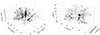 |
Fig. B.1. Illustration of how supergalactic coordinates distort the true position of galaxies. Here we show the distribution of exactly the same galaxies as in GAEA V2 but in a different coordinates system; the same area in the RA-DEC plane is shown in Fig. 1 (bottom-left panel). Left: Distribution of galaxies in supergalactic SGX-SGY-SGZ coordinates (includes elongation along the line of sight). Right: Same as left but in GAEA coordinate system x-y-z. |
In this Appendix, we check how much the filaments extracted from a galaxy distribution close to the observed one differ from the filaments obtained from the original galaxy distribution (without line-of-sight effects, in the Cartesian coordinates x-y-z of the model and without mimicking the selection function). We call the last filament structure (FS) ‘true’. We call filaments extracted by the distribution of galaxies close to observational ones ‘distorted’.
For GAEA V1, GAEA V2, and GAEA V3 we separately identified not only the filaments described in Sect. 3.1 but also a ‘true filaments system’ via the distribution of all galaxies with ![Mathematical equation: $ \log_{10} [\mathrm{M}_{\star} / \rm{M}_{{\odot}} ] > 8.3 $](/articles/aa/full_html/2024/10/aa50825-24/aa50825-24-eq37.gif) (e.g. without consideration of the selection function, the number of samples is significantly higher) in Cartesian coordinates of model x-y-z with a 4σ persistence level.
(e.g. without consideration of the selection function, the number of samples is significantly higher) in Cartesian coordinates of model x-y-z with a 4σ persistence level.
First of all, we inspected how much the filament membership determination depends on the way filaments are extracted (true vs distorted). This test is critical to obtain and estimate on the error of determining whether the galaxy belongs to the filament. The top panel of Fig. B.2 represents the confusion matrix for the classification of galaxies in GAEA-all samples. 18% of galaxies are members of the filaments and 51% are non-filament members according to both FSs. A distorted filament structure gives the correct galaxy status in more than 70% of cases. The remaining cells show errors in the definition, and their inequality is due to the fact that the true filamentous structure was extracted from a large number of samples with the same level of persistence, which makes it more detailed.
In addition to the status itself (inside or outside), we are also interested in how much the distorted distribution of galaxies helps restore the exact position of the filament axis. To check this, we calculate for each galaxy from GAEA-all the distance to the nearest filaments in true and distorted FS and compare these distances in the bottom panel of Fig. B.2. Since we do not observe a concentration of points around the line of equality, we conclude that the distorted filaments poorly reflect the true positions of the filament axes and have a significant effect on tests based on the distance to the filaments.
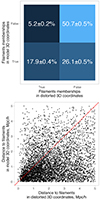 |
Fig. B.2. The correspondence between ‘true‘ and ‘distorted‘ filament identification. Left: Confusion matrix for classification of GAEA-all galaxies as filaments members according to filaments identified in SGX-SGY-SGZ (see Sect. 3.1) with distortion along line-of-sight (x-axis) and according to filaments identified for GAEA-all without mimicking of the selection function (see Sect. 2.2.1) in x-y-z (‘true‘ filaments, y-axis). The bottom left panel represents the fraction of galaxies identified as filament members according to both filament systems. The right top panel represents the fraction of galaxies identified as field members according to both filaments systems. The left top and bottom right panels represent inconsistency in the classification of filament members. Right: Comparison of distances for the indicated filament systems for each galaxy from GAEA-all in 3D. The red line represents the equality line. |
We additionally note that these conclusions are true for the close-to-observer regions, like Virgo and may differ for more distant ones.
Appendix C: Comparing the HI/H2 deficiency definition
For consistency between simulations and observations, in Sect. 4.2, we use a simplified definition of gas content that only includes stellar mass dependence. Here, we compare the obtained values with the values used in Castignani et al. (2022b). Figure C.1 shows that the data are in good agreement for HI and systematically underestimated values for H2. Given the overall small discrepancies, our simplified adopted definition does not negatively affect the analysis.
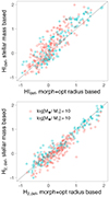 |
Fig. C.1. HI (top) and H2 (bottom) deficiency defined in this work and in Castignani et al. (2022b). |
Appendix D: Influence of the line-of-sight effects on the results
The effects described in Appendix B may also influence the results of this work. In the main paper, we use the distorted filament system (FS) for a straightforward comparison with observational data. Here we check that our results are not affected when considering the position of filaments without line-of-sight distortions.
In Appendix B we have shown that the distorted FS does a good job in classifying galaxies (inside or outside of filaments) but cannot reflect the exact position of the filament axis. Therefore, we expect that the results of Fig. 10 should be less affected than the results in Fig. 11.
Figure D.1 shows the analogue of the Fig. 10 but considering the ’true’ filaments. We again do not recover the difference in HI or H2-deficiency for galaxies inside or outside filaments with controlled halo mass, so elongation along line-of-sight does not affect this conclusion.
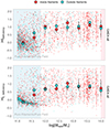 |
Fig. D.1. Same as Fig. 10 but with the classification of galaxies inside or outside filaments performed according to the FS identified without consideration of line-of-sight effects. |
Figure D.2 shows the comparison between HI-/H2-deficiency profiles for the distorted and ‘true‘ filaments. Focusing on filament galaxies, in the case of the distorted FS both profiles have a rather linear decrease with increasing distance from the filament spine; when considering instead the true filaments, the decrease follows an exponential decline. However, overall this does not affect the main results: a dependency of HI or H2 deficiency as a function of distance from the filament spine is recovered only for filaments and does not exist for pure filament.
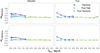 |
Fig. D.2. HI- or H2 deficiency (median values and 1σ significance interval) as a function of 3D distance to the nearest filament including line-of-sight distortions (left panels, full analogue of Fig. 11) and excluding them (right panels). |
All Tables
Number of galaxies with HI measurements above the gas mass completeness limit in C22, GAEA-mock, and all in each environment separately. The model data provides the median number of samples among the three halos under consideration.
All Figures
|
Fig. 1. Distribution of galaxies around the Virgo cluster (top-left panel, from Castignani et al. 2022b) and around the three Virgo-like clusters in the GAEA model (top right: GAEA V1, bottom left: GAEA V2, bottom right: GAEA V3) in celestial coordinates (corresponding to the GAEA-all sets; Sect. 4.1). The label of each panel indicates the mass of Virgo or of the Virgo-like halos. Each point is a galaxy with |
| In the text | |
|
Fig. 2. The scaling relation between MHI (top) and MH2 (bottom) as a function of stellar mass for observations. Red triangles show measurements, and crosses show upper limits. The solid red line shows the adopted level of completeness limits of the observations for HI (Eq. (1)) and H2 (Eq. (2)) masses, respectively. Shaded areas show the scaling relations for C22 (light blue, Eq. (3) in the top panel, Eq. (4) in the bottom panel) and for GAEA (light grey, Eq. (5) in the top panel, Eq. (6) in the bottom panel). |
| In the text | |
|
Fig. 3. Schematic view of the steps needed to obtain the final sample for both the model (GAEA-all, GAEA-mock) and the observed sample (C22). Each step is described in the main text (Sects. 2, 3, 4). |
| In the text | |
|
Fig. 4. The amount of HI-content in galaxies in clusters, filaments, and pure field. Top: MHI as a function of stellar mass in different environments, indicated on top of each panel. The GAEA model data are shown with circles: small circles represent the GAEA-all set, and big circles represent one of the 300 realisations of the GAEA-mock sample. Big triangles show the C22 data. In all the samples, each point is coloured by sSFR. In each panel, the solid grey line shows the MHI − M⋆ scaling relation (Eq. (5)), the dotted line shows the 0.5 dex indent to highlight HI-deficiency zone. The faint red line represents HI-mass completeness limit from Eq. (1). Bottom: Fractions of HI-deficient galaxies (see Sect. 4.2) with 1σ confidence interval as a function of stellar mass. |
| In the text | |
|
Fig. 5. HI-deficiency cumulative distribution function for GAEA-all (three lines for GAEA-all V1, GAEA-all V2 and GAEA-all V3); GAEA-mock (300 lines); and C22 split into the different environments and two mass bins (low-mass log10[M⋆/M⊙]< 10 and massive galaxies log10[M⋆/M⊙]> 10). In each plot, the median values with a 1σ confidential interval are reported. The grey vertical line shows the 0.5 HI-deficiency level as a level adopted to consider a galaxy as HI-deficient. |
| In the text | |
|
Fig. 6. The amount of H2-content in galaxies in clusters, filaments, and pure field. Top: MH2 as a function of stellar mass in the different environments. Panels, colours, and symbols are as in Fig. 4. Bottom: Fractions of H2-deficient galaxies in each environment by mass bins. Panels, colours, and symbols are as in Fig. 4. |
| In the text | |
|
Fig. 7. H2-deficiency distributions (CDF) and median values with 1σ confidential interval. The caption is the same as Fig. 5. The number of samples is presented in Table. 2. |
| In the text | |
|
Fig. 8. H2, deficiency–HIdeficiency relations for low-mass (top) and massive (bottom) galaxies in clusters (left), filaments (middle), and the pure field (right). GAEA-mock data is represented by big circles, GAEA-all data by small circles, and C22 data by triangles. Each point of the GAEA-mock/C22 is coloured by sSFR. The vertical and horizontal lines show 0.5 dex deficiency levels used to separate gas normal from gas deficient galaxies. |
| In the text | |
|
Fig. 9. Schematic representation of filament composition by galaxies in groups of different sizes and pure filament galaxies (i.e. alone in their halo; top panel). The proportion of galaxies in groups with 15 < Nmem < 50, 5 < Nmem < 15, and 1 < Nmem < 5 members and pure filament in total filaments population, respectively (bottom panel), taking into account the selection function. |
| In the text | |
|
Fig. 10. The dependency of atomic and molecular content at fixed halo mass for galaxies inside and outside filaments. Top: HI-deficiency as a function of the host halo mass Mhalo in GAEA-all. Colour coding reflects the position concerning filaments: inside or outside. Big circles show median values with 1σ confidential interval for galaxies inside and outside filaments in each mass bin (median values were estimated for similar Mhalo distribution for haloes inside and outside filaments by bootstrapping). On the background, typical pure filament/pure field (90%-quantile) and clusters of halo masses are highlighted. Bottom: Same but for H2-deficiency. |
| In the text | |
|
Fig. 11. HI- or H2-deficiency (median values and 1σ significance interval) as a function of 3D distance to the nearest filament in GAEA-all for filaments, the pure filament, and pure fields (top panels), and members of groups of different sizes: 1 < Nmem < 5, 5 < Nmem < 15, 15 < Nmem< 50 (bottom panels). |
| In the text | |
|
Fig. B.1. Illustration of how supergalactic coordinates distort the true position of galaxies. Here we show the distribution of exactly the same galaxies as in GAEA V2 but in a different coordinates system; the same area in the RA-DEC plane is shown in Fig. 1 (bottom-left panel). Left: Distribution of galaxies in supergalactic SGX-SGY-SGZ coordinates (includes elongation along the line of sight). Right: Same as left but in GAEA coordinate system x-y-z. |
| In the text | |
|
Fig. B.2. The correspondence between ‘true‘ and ‘distorted‘ filament identification. Left: Confusion matrix for classification of GAEA-all galaxies as filaments members according to filaments identified in SGX-SGY-SGZ (see Sect. 3.1) with distortion along line-of-sight (x-axis) and according to filaments identified for GAEA-all without mimicking of the selection function (see Sect. 2.2.1) in x-y-z (‘true‘ filaments, y-axis). The bottom left panel represents the fraction of galaxies identified as filament members according to both filament systems. The right top panel represents the fraction of galaxies identified as field members according to both filaments systems. The left top and bottom right panels represent inconsistency in the classification of filament members. Right: Comparison of distances for the indicated filament systems for each galaxy from GAEA-all in 3D. The red line represents the equality line. |
| In the text | |
|
Fig. C.1. HI (top) and H2 (bottom) deficiency defined in this work and in Castignani et al. (2022b). |
| In the text | |
|
Fig. D.1. Same as Fig. 10 but with the classification of galaxies inside or outside filaments performed according to the FS identified without consideration of line-of-sight effects. |
| In the text | |
|
Fig. D.2. HI- or H2 deficiency (median values and 1σ significance interval) as a function of 3D distance to the nearest filament including line-of-sight distortions (left panels, full analogue of Fig. 11) and excluding them (right panels). |
| In the text | |
Current usage metrics show cumulative count of Article Views (full-text article views including HTML views, PDF and ePub downloads, according to the available data) and Abstracts Views on Vision4Press platform.
Data correspond to usage on the plateform after 2015. The current usage metrics is available 48-96 hours after online publication and is updated daily on week days.
Initial download of the metrics may take a while.