Binary black hole mergers from Population III star clusters

Benedetta Mestichelli; Michela Mapelli; Stefano Torniamenti; Manuel Arca Sedda; Marica Branchesi; Guglielmo Costa; Giuliano Iorio; Filippo Santoliquido

doi:10.1051/0004-6361/202450667

Home

All issues

Volume 690 (October 2024)

A&A, 690 (2024) A106

Full HTML

Open Access

Issue		A&A Volume 690, October 2024


Article Number		A106
Number of page(s)		18
Section		Galactic structure, stellar clusters and populations
DOI		https://doi.org/10.1051/0004-6361/202450667
Published online		02 October 2024

A&A, 690, A106 (2024)

Binary black hole mergers from Population III star clusters

Benedetta Mestichelli¹^,2^,5^★, Michela Mapelli²^,3^,4, Stefano Torniamenti², Manuel Arca Sedda¹^,5, Marica Branchesi¹^,5, Guglielmo Costa⁶, Giuliano Iorio³^,4 and Filippo Santoliquido¹^,5

¹ Gran Sasso Science Institute (GSSI), Viale Francesco Crispi 7, 67100 L’Aquila, Italy
² Institut für Theoretische Astrophysik, ZAH, Universität Heidelberg, Albert-Ueberle-Straße 2, 69120 Heidelberg, Germany
e-mail: mapelli@uni-heidelberg.de; stefano.torniamenti@uni-heidelberg.de
³ Physics and Astronomy Department Galileo Galilei, University of Padova, Vicolo dell’Osservatorio 3, 35122 Padova, Italy
⁴ INFN – Padova, Via Marzolo 8, 35131 Padova, Italy
⁵ INFN, Laboratori Nazionali del Gran Sasso, 67100 Assergi, Italy
⁶ Univ Lyon, Univ Lyon1, ENS de Lyon, CNRS, Centre de Recherche Astrophysique de Lyon UMR5574, 69230 Saint-Genis-Laval, France

^★ Corresponding author; benedetta.mestichelli@gssi.it

Received: 9 May 2024
Accepted: 7 August 2024

Abstract

Binary black holes (BBHs) that are born from the evolution of Population III (Pop. III) stars are one of the main high-redshift targets for next-generation ground-based gravitational-wave (GW) detectors. Their predicted initial mass function and lack of metals make them the ideal progenitors of black holes above the upper edge of the pair-instability mass gap, that is, with a mass higher than ~134 (241) M_⊙ for stars that become (or do not become) chemically homogeneous during their evolution. We investigate the effects of cluster dynamics on the mass function of BBHs that are born from Pop. III stars by considering the main uncertainties on the mass function of Pop. III stars, the orbital properties of the binary systems, the star cluster mass, and the disruption time. In our dynamical models, at least ~5% and up to 100% BBH mergers in Pop. III star clusters have a primary mass m₁ above the upper edge of the pair-instability mass gap. In contrast, only ≲3% isolated BBH mergers have a primary mass above the gap, unless their progenitors evolved as chemically homogeneous stars. The lack of systems with a primary and/or secondary mass inside the gap defines a zone of avoidance with sharp boundaries in the plane of the primary mass-mass ratio. Finally, we estimate the merger rate density of BBHs. In the most optimistic case, we find a maximum of ℛ ~ 200 Gpc^-3 yr^-1 at ɀ ~ 15 for BBHs that formed via dynamical capture. For comparison, the merger rate density of isolated Pop. III BBHs is ℛ ≤ 10 Gpc⁻³ yr⁻¹ for the same model of Pop. III star formation history.

Key words: black hole physics / gravitational waves / stars: black holes / stars: Population III / galaxies: star clusters: general

© The Authors 2024

Open Access article, published by EDP Sciences, under the terms of the Creative Commons Attribution License (https://creativecommons.org/licenses/by/4.0), which permits unrestricted use, distribution, and reproduction in any medium, provided the original work is properly cited.

This article is published in open access under the Subscribe to Open model. Subscribe to A&A to support open access publication.

1 Introduction

The first generation of stars is called Population III (Pop. III) stars. They formed from zero-metallicity gas (Haiman et al. 1996; Tegmark et al. 1997; Yoshida et al. 2003), and their initial mass function (IMF) most likely included a larger contribution from massive stars than from stellar populations in the local Universe (Stacy & Bromm 2013; Susa et al. 2014; Hirano et al. 2015; Jaacks et al. 2019; Sharda et al. 2020; Liu & Bromm 2020a,b; Wollenberg et al. 2020; Chon et al. 2021; Tanikawa et al. 2021b; Jaura et al. 2022; Prole et al. 2022). Since Pop. III stars lack metals, their mass loss through stellar winds is less efficient. Consequently, the mass of their compact remnants can be close to their zero-age main-sequence (ZAMS) mass (Heger et al. 2002; Kinugawa et al. 2014, 2016; Hartwig et al. 2016; Belczynski et al. 2017; Tanikawa et al. 2021b,a, 2022, 2023; Costa et al. 2023; Santoliquido et al. 2023; Tanikawa 2024). We therefore expect Pop. III stars to efficiently produce intermediate-mass black holes (IMBHs), that is, black holes (BHs) in the mass range between 10² M⊙ and 10⁵ M_⊙ (Madau & Rees 2001; Woosley et al. 2002; Miller & Colbert 2004; Liu & Bromm 2020b; Kinugawa et al. 2021; Tanikawa et al. 2021b,a, 2022, 2023; Tanikawa 2024). However, the exact shape of the Pop. III IMF is still largely unknown. The star formation history of these stars is poorly constrained as well. In the ΛCDM model, Pop. III stars begin to form at z ≥ 30, but reach a peak in their star formation rate at z ∼ 15–20 (for a recent review of the Pop. III star formation, see Klessen & Glover 2023).

Recent binary evolution simulations showed that very few IMBHs born from Pop. III stars merge with other (IM)BHs (Tanikawa et al. 2021b,a, 2022, 2023; Costa et al. 2023; Tanikawa 2024). The main reason is that very massive Pop. III stars reach large radii (>100 R_⊙) during their life and thus they either collide prematurely with their companion star before becoming BHs or produce loose binary black holes (BBHs), whose initial semimajor axis is too wide for them to merge within the lifetime of the Universe.

However, if some of the Pop. III stars formed in stellar clusters, we expect stellar dynamics to efficiently couple and harden these massive BBHs (Heggie 1975). Hence, star cluster dynamics might significantly boost the BBH merger rate from Pop. III stars (Wang et al. 2022). The first star clusters were embedded in dark matter halos of ∼10⁷ M_⊙ (Reed et al. 2007; Sakurai et al. 2017), which could host star clusters with M_cl ≲ 10⁵ M_⊙ (Bromm & Clarke 2002; Sakurai et al. 2017; Wang et al. 2022). N-body models indicate that the presence of these dark matter halos can prevent the star cluster from disruption and keep it bound long enough to dynamically form and harden BBHs (Wang et al. 2022).

Current gravitational-wave (GW) interferometers are able to detect BBH mergers up to a redshift z ∼ 2 (Abbott et al. 2020, 2023a,b). Thus, they can detect BBH mergers from Pop. III stars only when these occur at low redshift, with a long delay time. We expect these events to be outnumbered by BBH mergers originating from Population I and II stars at low redshift (Santoliquido et al. 2023). However, starting from the next decade, third-generation GW detectors such as Cosmic Explorer (Reitze et al. 2019) and the Einstein Telescope (Punturo et al. 2010) will have a much larger instrumental horizon and observe BBH mergers up to a redshift of ∼100 (Kalogera et al. 2021; Branchesi et al. 2023). Mergers of BBHs from Pop. III stars will be one of the most sought-after sources of GWs in the high- redshift Universe (Kalogera et al. 2021; Ng et al. 2021, 2022a,b; Périgois et al. 2021; Santoliquido et al. 2023, 2024).

In this work, we explore the hierarchical mergers of Pop. III BBHs in dense star clusters while probing a wide range of initial conditions for their IMFs and the formation channels of firstgeneration BBHs. We investigate the impact of the dynamical environment on the build-up and merger of IMBHs. For this purpose, we employ the semi-analytic code FASTCLUSTER, which was conceived to model hierarchical BBH mergers in star clusters while efficiently exploring the parameter space that this process involves. The paper is structured as follows. Section 2 presents the initial conditions and outlines the numerical code. In Sect. 3, we describe our main results. Section 4 discusses the main implications of our results, including the BBH merger rate density, and Sect. 5 summarizes our conclusions.

2 Methods

We used the semi-analytic code FASTCLUSTER (Mapelli et al. 2021, 2022; Vaccaro et al. 2024; Torniamenti et al. 2024), which integrates the effect of BBH dynamical hardening and GW emission while capturing the main physical processes that drive the evolution of the host star cluster. A complete description of FASTCLUSTER can be found in Mapelli et al. (2021, 2022), and Torniamenti et al. (2024). In the following, we summarize the details of the setup and initial conditions considered for this work.

2.1 Stellar tracks for Population III stars

We produced our first-generation (single and binary) BHs with the binary population synthesis code SEVN (Spera et al. 2019; Mapelli et al. 2020; Iorio et al. 2023), which calculates the stellar evolution by interpolating a set of precomputed single stellar tracks and models the main binary interaction processes by means of semi-analytic prescriptions (Hurley et al. 2002; Iorio et al. 2023).

We computed the Pop. III star tracks with the stellar evolution code PARSEC (Bressan et al. 2012; Chen et al. 2015; Costa et al. 2019). Specifically, we distinguished two different evolutionary paths of Pop. III stars: default, and chemically homogeneous evolution (CHE). We evolved the default tracks by assuming initially nonspinning stars with an initial hydrogen abundance X = 0.751, a helium abundance Y = 0.2485 (Komatsu et al. 2011), and a metallicity Z = 10^–11 (Tanikawa et al. 2021b; Costa et al. 2023), and by considering the mass range between 2 and 600 M_⊙.

For the CHE stars, we simulated a sample of pure-He tracks considering initial masses ranging from 0.36 to 350 M_⊙, with an initial hydrogen abundance X = 0, a helium abundance Y = 1 – Z, and a metallicity Z = 10^–6. This metallicity is similar to the metal content we find in He cores of Pop. III stars after the main-sequence phase. We ran these tracks as a proxy for CHE stars, which are deemed to be the result of fast-spinning metalpoor stars that become fully mixed already near the end of the main sequence (Mandel & de Mink 2016; de Mink & Mandel 2016; Marchant et al. 2016; Riley et al. 2022). In the context of Pop. III stars, it is important to explore the possibility of rapidly rotating stars because simulations showed that most of them have a rotational velocity between 50% and 100% of their Keplerian velocity (Stacy & Bromm 2013). Like our pure-He stars, CHE stars remain mostly compact during their entire evolution (de Mink & Mandel 2016). Since in our simplified treatment of CHE stars we skipped the integration of the hydrogen main sequence, we then increased the BBH formation time by a factor equal to the duration of the main sequence. We refer to Appendix A.2 and to Costa et al. (2023) and Santoliquido et al. (2023) for more details about our Pop. III stellar tracks.

2.2 Population synthesis with SEVN

The population synthesis code SEVN assigns the final fate to each star based on a formalism for core-collapse and (pulsational) pair-instability supernovae. Namely, we adopted the rapid model for core-collapse supernovae (Fryer et al. 2012), which enforces a mass gap between neutron stars and BHs, and the fitting formulas by Mapelli et al. (2020) for (pulsational) pair-instability supernovae. Our model for pair instability results in a mass gap in the BH mass function between ∼86 and 241 M_⊙ for the default single-star models (see Fig. 6 of Costa et al. 2023). For the CHE models, the pair-instability mass gap is between ∼46 and ∼134 M_⊙ because these models evolve without H-rich envelope after the main sequence (see Fig. 17 of Santoliquido et al. 2023).

For each of our samples (default and CHE), we used SEVN in single- and binary-star mode. The single-star setup allowed us to generate single BHs for the dynamical BBH sample (see Sect. 2.3.2), and the binary-star mode was used to produce our isolated and original BBHs (see Section 2.3.1).

2.2.1 Single and binary initial conditions

In the single-star set up, we ran six simulations with SEVN. Because of the uncertainties on the IMF of Pop. III stars, we ran each model with a Kroupa (Kroupa 2001) (kro1), a Larson (Larson 1998) (lar1 and lar5che), a top-heavy (e.g., Liu & Bromm 2020a) (top1), and a log-flat (e.g., Jaura et al. 2022; Hartwig et al. 2022) (log1 and log1che) IMF. We refer to Costa et al. (2023) and to our Appendix A for a description of these IMFs.

For the binary-star mode, we did not run new SEVN models, but rather reused the outputs of the simulations presented by Costa et al. (2023). These simulations assumed a variety of initial conditions that encompass the uncertainties on Pop. III binary star systems, and they are summarized in Table 1. Namely, they considered the same IMFs as for the single star runs. For the mass ratios, they considered a uniform sampling (log3), the distribution by Sana et al. (2012) resulting from fitting formulas to nearby massive binary stars (kro1, lar1, log1, log1che, log2, and top1), or the results by Stacy & Bromm (2013) (kro5, lar5, lar5che, log4, log5, and top5). For the initial orbital period distribution, they assumed either the fit by Sana et al. (2012) (kro1, lar1, log1, log1che, log3, log4, and top1) or the results by Stacy & Bromm (2013) (kro5, lar5, lar5che, log2, log5, and top5). Finally, for the initial orbital eccentricities, they adopted either the fit by Sana et al. (2012) (kro1, lar1, log1, log1che, log3, and top1) or a thermal eccentricity distribution (kro5, lar5, lar5che, log2, log4, log5, and top5). We describe the setup of each run in our Appendix A.

In the following sections, we assume the model log1 (Costa et al. 2023) as our fiducial model. In Sect. 3.5, we show the results we found by adopting other initial conditions.

Table 1

Initial conditions for the stellar models.

2.2.2 Isolated binary black holes

Costa et al. (2023) only described the subsample of BBHs that merge over a timescale shorter than the lifetime of the Universe (measured by the Hubble time, t_H = 13.6 Gyr). Here, we call them isolated BBH mergers: BBHs that form from isolated binary stars that are not members of stellar clusters and evolve unperturbedly until they merge within tH = 13.6 Gyr. We further describe the isolated BBH sample in Appendix A. We only show the isolated BBHs for the sake of comparison.

2.3 Binary black holes in star clusters

We considered two channels for the first-generation BBHs in star clusters: dynamical (hereafter, Dyn) BBHs, and original (hereafter, Orig) BBHs. The former originate from single Pop. III stars and then pair up dynamically inside their host star cluster, whereas the latter are BBHs that form from the evolution of original binary systems of Pop. III stars. Binary systems that are already present in the initial conditions of our star cluster simulations and then evolve dynamically inside the cluster are called original binary systems. In stellar dynamics, they are usually referred to as primordial binaries (Goodman & Hut 1989), but we use the term original binaries here to avoid confusion with primordial BHs (Carr et al. 2016).

2.3.1 Original binary black holes

Original BBHs come from the binary-star simulations presented by Costa et al. (2023), who evolved several sets of Pop. III binary stars with the code SEVN (see Sect. 2.1).

We initialized the original BBHs by considering all the BBHs that formed in the simulations by Costa et al. (2023), including those with a delay time much longer than the Hubble time. The star-cluster dynamics can either ionize or harden these BBHs, depending on whether they are soft or hard binary systems (Heggie 1975). Thus, some of the wide BBH binaries in Costa et al. (2023) are likely to harden dynamically and merge within a Hubble time. In Appendix A, we provide additional details about them.

2.3.2 Dynamical binary black holes

Dynamical BBHs form via three-body interactions at the time of core-collapse of the star cluster, when the central density of the cluster is highest (Torniamenti et al. 2024). In the case of dynamical BBHs, we drew the masses of the primary BHs out of the SEVN single BH catalogs, that is, we assumed that these BHs come from the evolution of single stars. We assigned the primary and secondary BH masses using two different pairing functions that we describe below.

DynA: We sampled m1 uniformly, while m2 followed the probability distribution p(m₂) ∝ (m₁ + m₂)⁴, as found by O’Leary et al. (2016). As shown in Torniamenti et al. (2024), this sampling criterion can encompass the uncertainties connected with the BH pairing function, for instance, due to stochastic fluctuations, stellar and binary evolution, and BH-star interactions.
DynB: We sampled m₁ following the mass-pairing criterion adopted by Antonini et al. (2023) and based on Heggie (1975). This function describes the dynamical formation of hard BBHs through three-body encounters and systematically leads to the pairing of the most massive objects (for further details, see Appendices B and C).

We sampled the initial orbital eccentricity and semimajor axis of the dynamical BBHs from the distributions $\begin{array}{l} p (e) = 2 e, & with e \in [0, 1), \\ p (a) \propto a^{- 1}, & with a \in [1, 10^{3}] R_{⊙} . \end{array}$ $\matrix{ {p(e) = 2e,} \hfill & {{\rm{with}}\,\,\,e \in [0,1),} \hfill \cr {p(a) \propto {a^{ - 1}},} \hfill & {{\rm{with}}\,\,a \in \left[ {1,{{10}^3}} \right]{{\rm{R}}_ \odot }.} \hfill \cr }$ (1)

These distributions are commonly used for hard binary systems in star clusters (Mapelli et al. 2021).

2.3.3 Spins of first-generation binary black holes

For both original and dynamical BBHs, we generated the dimensionless spin magnitudes χ₁ and χ₂ from a Maxwellian distribution with σ_χ = 0.05 and truncated at χ = 1. This choice for the spin magnitudes is a toy model matching the properties of LIGO–Virgo BBHs by construction (Abbott et al. 2023c). The spin directions were drawn isotropically over a sphere because dynamical interactions remove any alignment of the spins with the angular momentum of the binary system (Rodriguez et al. 2016).

2.3.4 Additional checks for first-generation binary black holes

For both original and dynamical BBHs, we verified whether the binary was hard, that is, whether the binding energy of the BBH was higher than the average kinetic energy of a star, $E_{b} = \frac{G m_{1} m_{2}}{2 a} > 〈 E_{k} 〉 = \frac{1}{2} m_{*} σ^{2},$ ${E_{\rm{b}}} = {{G{m_1}{m_2}} \over {2a}} > \langle {E_{\rm{k}}}\rangle = {1 \over 2}{m_*}{\sigma ^2},$ (2)

where m₁ and m₂ are the masses of primary and secondary stars at the ZAMS (BHs) in the case of original (dynamical) BBHs, and m_* is the average mass of a star in the cluster (depending on the chosen IMF) and σ the three-dimensional velocity dispersion. We neglected dynamical exchanges, which might enhance the mass of the BBH components. On the other hand, the effect of dynamical exchanges is already taken into account in the BBH formation rate of model DynB (see Appendix B). When the binary was soft, it was not integrated further because we assumed that it is disrupted by dynamical interactions.

After drawing the masses, we verified whether the BHs were expelled from the cluster by a supernova kick. We estimated the natal kick as previously done by Mapelli et al. (2021), $v_{SN} = v_{H 05} \frac{〈 m_{NS} 〉}{m_{BH}},$ ${v_{{\rm{SN}}}} = {v_{{\rm{H}}05}}{{\langle {m_{{\rm{NS}}}}\rangle } \over {{m_{{\rm{BH}}}}}},$ (3)

where 〈m_NS〉 = 1.33 M⊙ is the average neutron star mass (Özel & Freire 2016), m_BH is the BH mass, and v_H05 is a number drawn from a Maxwellian distribution with σ_v = 265 km s^–1. This quantity was compared to the escape velocity of the cluster, which we computed as (Georgiev et al. 2009) $v_{esc} = 40 km s^{- 1} {(\frac{M_{cl}}{10^{5} M_{⊙}})}^{1 / 3} {(\frac{ρ}{10^{5} M_{⊙} {pc}^{- 3}})}^{1 / 6},$ ${v_{{\rm{esc}}}} = 40{\rm{km}}{{\rm{s}}^{ - 1}}{\left( {{{{M_{{\rm{cl}}}}} \over {{{10}^5}{{\rm{M}}_ \odot }}}} \right)^{1/3}}{\left( {{\rho \over {{{10}^5}{{\rm{M}}_ \odot }{\rm{p}}{{\rm{c}}^{ - 3}}}}} \right)^{1/6}},$ (4)

where M_cl is the mass of the cluster, and ρ is the density at the half-mass radius. When for the primary or secondary mass in a dynamical BBH v_SN > v_sc, the binary was no longer integrated. In the case of an original BBH, the orbital evolution of the binary was computed outside the cluster.

2.4 Orbital evolution and Nth generation binary black holes

We evolved the semimajor axis a and eccentricity e using the formalism presented by Mapelli et al. (2021), where dynamical hardening (Heggie 1975) and GW decay (Peters 1964) are taken into account, $\begin{array}{l} \frac{d a}{d t} = - 2 π ξ \frac{G ρ_{c}}{σ} a^{2} - \frac{64}{5} \frac{G^{3} m_{1} m_{2} (m_{1} + m_{2})}{c^{5} a^{3} {(1 - e^{2})}^{7 / 2}} f_{1} (e), \\ \frac{d e}{d t} = 2 π ξ κ \frac{G ρ_{c}}{σ} a - \frac{304}{15} e \frac{G^{3} m_{1} m_{2} (m_{1} + m_{2})}{c^{5} a^{4} {(1 - e^{2})}^{5 / 2}} f_{2} (e), \end{array}$ $\matrix{ {} \hfill & {{{{\rm{d}}a} \over {{\rm{d}}t}} = - 2\pi \xi {{G{\rho _{\rm{c}}}} \over \sigma }{a^2} - {{64} \over 5}{{{G^3}{m_1}{m_2}\left( {{m_1} + {m_2}} \right)} \over {{c^5}{a^3}{{\left( {1 - {e^2}} \right)}^{7/2}}}}{f_1}(e),} \hfill \cr {} \hfill & {{{{\rm{d}}e} \over {{\rm{d}}t}} = 2\pi \xi \kappa {{G{\rho _{\rm{c}}}} \over \sigma }a - {{304} \over {15}}e{{{G^3}{m_1}{m_2}\left( {{m_1} + {m_2}} \right)} \over {{c^5}{a^4}{{\left( {1 - {e^2}} \right)}^{5/2}}}}{f_2}(e),} \hfill \cr }$ (5)

where ρ_c is the core density, ξ is a numerically calibrated constant that we fixed to ξ = 3 (Hills 1983; Quinlan 1996; Sesana et al. 2006), and κ = de/dln (1 /a). The functions f₁(e) and f₂(e) were defined by Peters (1964) as $\begin{array}{l} f_{1} (e) = (1 + \frac{73}{24} e^{2} + \frac{37}{96} e^{4}), \\ f_{2} (e) = (1 + \frac{121}{304} e^{2}) . \end{array}$ $\matrix{ {} \hfill & {{f_1}(e) = \left( {1 + {{73} \over {24}}{e^2} + {{37} \over {96}}{e^4}} \right),} \hfill \cr {} \hfill & {{f_2}(e) = \left( {1 + {{121} \over {304}}{e^2}} \right).} \hfill \cr }$ (6)

When a BBH merged within the lifetime of its cluster (see Sect. 2.6), we computed the spin and mass of the remnant using the fitting formulas by Jiménez-Forteza et al. (2017). Moreover, we estimated the magnitude of the relativistic kick v_k experienced by the remnant with Eq. (12) from Lousto et al. (2012). When v_k < v_esc (with v_esc from Eq. (4)), the merger remnant remains inside the cluster and is able to pair up again, otherwise, it is ejected and we no longer considered it.

We generated the nth-generation secondary BHs using the pairing criteria described in Sect. 2.3.2. We assumed that the secondary BH always belonged to the first generation and m₂ ∈ [m_min, max(m_1,1g)], with max(m_1,1g) the maximum mass of a first-generation primary BH. Torniamenti et al. (2024) also considered the case in which the secondary BH was an nth-generation BH and found no substantial differences.

We repeated the hierarchical merger process until one of the following conditions was reached: the merger remnant was ejected from the star cluster, the cluster evaporated, no BHs were left inside the cluster, or z_min (Sect. 2.6).

2.5 Ejection by three-body encounters

It is essential to know whether a BBH is ejected from its parent cluster as a consequence of a binary-single star scatter before it can merge. When this occurs, the BBH merges outside the cluster and the final stages of its evolution are only driven by GW decay, without dynamical hardening. In FASTCLUSTER , we used a simple argument based on energy exchanges during binary-single star encounters to estimate this process (Miller & Hamilton 2002). Specifically, we expect that the gravitational recoil induced by a binary-single encounter can lead to the ejection of a BBH when its semimajor axis is shorter than (Miller & Hamilton 2002) $a_{ej} = \frac{2 ξ m_{*}^{2}}{{(m_{1} + m_{2})}^{3}} \frac{G m_{1} m_{2}}{v_{esc}^{2}} .$ ${a_{{\rm{ej}}}} = {{2\xi m_ * ^2} \over {{{\left( {{m_1} + {m_2}} \right)}^3}}}{{G{m_1}{m_2}} \over {v_{{\rm{esc}}}^2}}.$ (7)

For comparison, we estimated the maximum semimajor axis for which the shrinking by emission of GWs starts to dominate the shrinking by dynamical hardening (Baibhav et al. 2020), $a_{GW} = {[\frac{32 G^{2}}{5 π ξ c^{5}} \frac{σ m_{1} m_{2} (m_{1} + m_{2})}{ρ_{c} {(1 - e^{2})}^{7 / 2}} f_{1} (e)]}^{1 / 5} .$ ${a_{{\rm{GW}}}} = {\left[ {{{32{G^2}} \over {5\pi \xi {c^5}}}{{\sigma {m_1}{m_2}\left( {{m_1} + {m_2}} \right)} \over {{\rho _{\rm{c}}}{{\left( {1 - {e^2}} \right)}^{7/2}}}}{f_1}(e)} \right]^{1/5}}.$ (8)

Statistically, we expect that the BBH merges inside the cluster when a_GW > a_ej, which is the criterion we adopted in FASTCLUSTER (these mergers are labeled InCl). Otherwise, we assumed that the BBH is ejected and merges in the field (label Ej3B).

2.6 Properties of the star clusters

Cosmological hydrodynamic simulations (Sakurai et al. 2017) indicate that Pop. III star clusters tend to form in dark matter halos with mDM ∼ 10⁷ M_⊙. These star clusters form at epochs up to z ∼ 20, and present typical masses M_cl ≲ 10⁵ M_⊙ (Sakurai et al. 2017; Wang et al. 2022). At the same time, magnetohydrodynamic simulations (He et al. 2019) show that under conditions that reproduce those expected in high-redshift galaxies, molecular clouds up to ∼10⁵ M_⊙ produce a majority of star clusters with ∼10⁴ M_⊙.

We considered both high-mass (HM) and low-mass (LM) star clusters, assuming that they both form at z = 20. We drew the initial cluster masses from a log-normal distribution with a mean 〈log₁₀ M_cl/M_⊙〉 = 5.6 and 4.3 for HM and LM clusters, respectively, and a standard deviation σ_M = 0.4. We drew their density at the half-mass radius from a log-normal distribution with a mean 〈log₁₀ρ/(M_⊙ pc^–3)〉 = 3.7 and 3.3 for HM and LM clusters, respectively, and σ_ρ = 0.4. This choice of parameters for the HM clusters was inspired by Sakurai et al. (2017) and Wang et al. (2022), whereas for the LM clusters we adopted typical values for low-redshift young massive clusters (Mapelli et al. 2022). We consider a cosmology-motivated mass distribution in a follow-up work.

We integrated the star cluster evolution following the model in Torniamenti et al. (2024), based on the formalism presented in Antonini & Gieles (2020). We did not consider mass loss from tidal stripping from the host galaxy, but evolved the clusters until a minimum redshift zmin, at which we assumed them to be disrupted. After the disruption, the BBHs evolve and eventually merge in isolation. The results presented below were obtained taking z_min = 2. In Sect. 4.1, we compare them to results found with z_min = 10, 6.

2.7 Merger rate density

We estimated the BBH merger rate density using the semi- analytic code COSMOℛATE (Santoliquido et al. 2020, 2021), which combines catalogs of simulated BBH mergers with a chosen star formation rate density model. Specifically, the merger rate density in a comoving frame is computed as $ℛ = \int_{Z_{\max}}^{Z_{}} ψ (z^{'}) \frac{d t (z^{'})}{d z^{'}} [\int_{Z_{\min}}^{Z_{\max}} η (Z) ℱ (z^{'}, z, Z) d Z] d z^{'} .$ ${\cal R} = \int_{{Z_{\min }}}^{{Z_{\max }}} \psi \left( {z'} \right){{{\rm{d}}t\left( {z'} \right)} \over {{\rm{d}}z'}}\left[ {\int_{{Z_{\min }}}^{{Z_{\max }}} \eta (Z){\cal F}\left( {z',z,Z} \right){\rm{d}}Z} \right]{\rm{d}}z'.$ (9)

Here, ψ(z′) is the chosen star formation rate density; we chose the star formation history derived by the semi-analytic model of Hartwig et al. (2022), which traces individual Pop. III stars, and is calibrated on several observables from the local and high- redshift Universe. In Eq. (9), $d t (z^{'}) / d z^{'} = H_{0}^{- 1} {(1 + z^{'})}^{- 1} {[{(1 + z^{'})}^{3} Ω_{M} + Ω_{Λ}]}^{- 1 / 2}$ ${\rm{d}}t(z')/{\rm{d}}z' = H_0^{ - 1}{(1 + z')^{ - 1}}{[{(1 + {z^\prime })^3}{\Omega _M} + {\Omega _\Lambda }]^{ - 1/2}}$ , where H₀ is the Hubble parameter, and Ω_M and Ω_Λ are the matter and dark energy densities (Planck Collaboration VI 2020). The merger efficiency η(Z) is defined differently for original and dynamical BBHs. In the case of dynamical BBHs, we specify it as $η_{Dyn} (Z) = \frac{N_{merge,sim} (Z)}{N_{sim} (Z)} \frac{N_{BH} (Z)}{M_{cl, TOT} (Z)} .$ ${\eta _{{\rm{Dyn}}}}(Z) = {{{{\cal N}_{{\rm{merge,sim}}}}(Z)} \over {{{\cal N}_{{\rm{sim}}}}(Z)}}{{{{\cal N}_{{\rm{BH}}}}(Z)} \over {{M_{{\rm{cl}},{\rm{TOT}}}}(Z)}}.$ (10)

Here, N_merge,sim(Z) is the number of simulated BBH mergers, and N_sim(Z) is the number of simulated BBHs. N_BH(Z) is instead the number of BHs we expect to form from a stellar population, assuming a certain IMF and that all stars with ZAMS mass above 20 M_⊙ are BH progenitors. Finally, M_cl,TOT(Z) is the total initial mass of the simulated clusters.

In the case of original BBHs, we define the merger efficiency as $η_{Orig} (Z) = \frac{N_{merge, sim} (Z)}{N_{sim} (Z)} \frac{N_{TOT} (Z)}{M_{*} (Z)},$ ${\eta _{{\rm{Orig}}}}(Z) = {{{{\cal N}_{{\rm{merge}},{\rm{sim}}}}(Z)} \over {{{\cal N}_{{\rm{sim}}}}(Z)}}{{{{\cal N}_{{\rm{TOT}}}}(Z)} \over {{M_*}(Z)}},$ (11)

where the second ratio is a formation efficiency of the BBHs in our SEVN catalogs, where NTOT(Z) is the total number of BBHs and M_*(Z) is the total initial stellar mass. The term ℱ(z′, z, Z) is given by $ℱ (z^{'}, z, Z) = f_{CL} (z^{'}, M_{cl}) \frac{N (z^{'}, z, Z)}{N_{tot,Hubble} (Z)} p (z^{'}, Z),$ ${\cal F}\left( {z',z,Z} \right) = {f_{{\rm{CL}}}}\left( {z',{M_{{\rm{cl}}}}} \right){{{\cal N}\left( {z',z,Z} \right)} \over {{{\cal N}_{{\rm{tot,Hubble}}}}(Z)}}p\left( {z',Z} \right),$ (12)

where f_CL(z′, M_cl) is the fraction of the stellar mass that is contained in HM and LM clusters at redshift z′; we set f_CL = 1, assuming that all the stellar mass at z^′ is either included in HM or LM clusters. N(z′, z, Z) gives us the number of BBHs forming at redshift z^′ with metallicity Z and merging at redshift z, while N_tot,_Hubble(Z) is the total number of BBHs formed from a population with metallicity Z and merging within a Hubble time. Finally, since we fixed Z = 10—¹¹ (Z = 10^-6) for the default (CHE) stars, p(z′, Z) is a delta function different from zero only at Z = 10^–11 (Z = 10^–6).

3 Results

3.1 Dynamical versus isolated binary black holes

Figure 1 displays the primary and secondary mass distribution of dynamical BBH mergers. For comparison, we also show the isolated BBHs from Costa et al. (2023). We considered both log1 and log1che BBHs in HM clusters.

The star-cluster dynamics boosts the merger rate of Pop. III BBHs above the pair-instability mass gap by several orders of magnitude. For most BBH mergers, the primary and secondary members lie above the mass gap when we adopt the pairing function by Antonini et al. (2023): Model DynB (both log1 and log1che) yields almost no BBH with m₁ < 200 M_⊙.

We find a dramatic difference between isolated BBHs and dynamical BBHs: BBH mergers above the gap are rare in isolated BBHs, but they are common in dynamical BBHs. This difference is strongest in the case of model DynB (both with and without CHE): BBH mergers with m₁ above the mass gap are at least ∼98% of the dynamical BBHs (both with and without CHE), while they are much less common in isolated BBHs (at most ∼39% for CHE models). Model DynA, on the other hand, yields a percentage of BBH mergers above the gap spanning from ∼5% to ∼71%.

In the models with CHE (e.g., log1che), we find a smaller difference between isolated and dynamical BBHs above the gap than in the default models. CHE favors the merger of isolated BBHs above the mass gap because the stellar radii are compact throughout the entire stellar evolution (see the discussion by Santoliquido et al. 2023). This allows very massive stars to evolve in a tight binary system without colliding prematurely, so that they eventually produce massive tight BBHs.

Even in the CHE models, the star-cluster dynamics allows the pairing and merger of more massive BBHs and the formation of hierarchical chains that push m₁ up to ∼700 M_⊙. As above, the pairing criterion DynB definitely favors the formation and merger of BBHs with m1 above the upper-mass gap.

In Table 2, we present the fraction of BBH mergers with m1 above the pair-instability mass gap for all the simulated models. Dynamical BBHs (especially those paired with DynB) in general involve a primary BH above the gap. Models with a longer initial orbital period from Stacy & Bromm (2013) (those ending with 5 and log2) produce little or no merging systems with m₁ above the upper-mass gap in isolation; the effect of star-cluster dynamics is to efficiently harden these BBHs, and it causes them to merge.

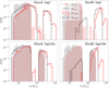Fig. 1

Distributions of primary (red) and secondary (black) masses of BBHs merging in HM clusters for log1 (upper panels) and log1che (lower panels). The shaded histograms show the results found by Costa et al. (2023) for isolated BBHs. The left column shows the results found with the pairing function DynA, and the right column shows the results with DynB.

3.2 Position of the pair-instability mass gap

Fig. 1 also shows that the position of the so-called pair-instability mass gap changes depending on whether we consider isolated binaries, dynamical binaries, or CHE (either with or without dynamics). In the isolated binaries (m1,iso and m2,iso in the upper panels), the mass gap starts at ∼50 M_⊙. In the dynamical binaries (both DynA and DynB) with log1 initial conditions (upper panels), the lower and upper edges of the mass gap are at ∼100 and ∼200 M_⊙, respectively. Finally, in the CHE case (log1che, lower panels), the lower and upper edges of the mass gap are at ∼50 and ∼135 M_⊙, respectively.

This difference is a direct consequence of the total mass of the star at the onset of core collapse in these three different cases. In our models we assume that when the star directly collapses into a BH, the mass of the BH is equal to the total mass of the star at the onset of collapse. Isolated binary systems that evolve into BBH mergers must undergo at least one mass-transfer episode during their life (Belczynski et al. 2016; Tanikawa et al. 2021b). This mass transfer efficiently removes the envelope of the donor star and leaves the He core naked. Thus, the lower (upper) edge of the pair-instability mass gap in isolated BBH mergers is ∼50 M⊙ (∼200 M_⊙) because this corresponds to the maximum (minimum) naked He core mass below (above) the gap.

In contrast, single Pop. III stars (or Pop. III stars in noninteracting binary systems) that do not develop a chemically homogeneous structure produce BHs with mass up to ∼90 M_⊙ below the pair-instability gap because they can retain a residual fraction of their H-rich envelope until the onset of the collapse; the mass of their BH is thus given by the sum of the He core mass and the residual H-rich envelope (Costa et al. 2021). These single Pop. III stars and noninteracting binary systems do not give birth to BBH mergers in the isolated binary evolution scenario because the former are not members of binary systems and the orbital periods of the latter are too long for them to merge via GW emission. In contrast, when these single stars evolve in a star cluster, their BHs can pair up dynamically with other BHs and lead to BBH mergers. This explains why the lower edge of the mass gap in the DynA and DynB cases is ∼90 M_⊙, which is much higher than in the isolated scenario.

Finally, in the CHE scenario, the stars become pure-He stars after the main sequence because they are very fast rotators (Maeder 1987; Woosley & Heger 2006). As a consequence, the masses of their BHs also result from the collapse of the He core because there is no H-rich envelope left after CHE. This explains why the mass gap is between 50 and 130 M_⊙, which are the masses of the He cores below and above the pair-instability mass gap. Unlike the other models, we do not see any difference in the location of the pair-instability mass gap between isolated binary evolution and dynamical evolution because all stars are naked He cores at collapse. Here, we made the assumption that metal-free massive stars are very fast rotators since their birth. If the only way to produce such fast rotators is via tidal spin-up in binary systems (de Mink & Mandel 2016; Marchant et al. 2016), then we would expect that models DynA and DynB log1che become similar to models DynA and DynB log1, accounting for the fact that single stars and stars in noninteracting binaries do not develop CHE via tidal spin up.

Table 2

Binary black hole mergers above the upper-mass gap.

3.3 Original versus dynamical binary black holes

Figure 2 shows the distribution of the mass ratio q of BBH mergers as a function of their primary mass for the log1 model. We show isolated binaries (Costa et al. 2023), original binaries, and dynamical binaries (for both pairing functions).

Overall, the distribution of m₁ − q for the original binaries is similar to that of the isolated binaries, but for one key difference: the dynamical hardening in stellar clusters boosts the merger rate of original BBHs above the pair-instability mass gap compared to isolated BBHs. Above the gap, original binaries behave more like dynamical BBHs than like isolated BBHs.

Model DynB predicts BBH mergers solely above the upper mass gap; this model leads to the pair-up of the most massive BHs in the star cluster. In this case, we find that the minimum primary mass of BBH mergers is ~200 M_⊙. Model DynA instead shows a milder effect of the dynamics onto the mass distribution of BBH mergers, with the majority of BBH mergers (~65%) below the upper-mass gap.

Figure 2 also shows that we expect several sharp features in the m₁ − q plot of both original and dynamical BBHs because of the pair-instability mass gap. Specifically, we expect a zone of avoidance in the m₁ − q plane, corresponding to the values for which m₁ is above the pair-instability mass gap and m₂ would be inside the mass gap. No such feature is apparent for isolated Pop. III BBH mergers because of the scarcity of mergers above the gap.

Figure 3 shows the same distributions for log1che. In this case, the distributions of isolated, original, and dynamical BBHs in the m₁ − q plane are more similar to each other because CHE enhances the fraction of mergers above the mass gap also for isolated BBHs. As a result, the isolated, original, and DynA models display similar percentages of BBH mergers above the upper-mass gap (~40 − 45%). In this case as well, model DynB stands out because it produces BBH mergers entirely above the pair-instability mass gap, much like in the log1 case (see Table 2).

3.4 Impact of the cluster properties

Figure 4 shows the primary mass distribution of multiple BBH merger generations obtained by simulating HM and LM clusters with log1. We do not show the log1che model because it yielded very similar results.

There are fewer BBH mergers in LM clusters in the region above m₁ ~ 600 M_⊙, and fewer systems generate a chain of mergers compared to HM clusters because LM clusters are less massive and less dense than HM clusters. As a consequence, their typical escape velocity is lower (υ_esc ~ 15 km s⁻¹). The effect of a lower escape velocity is twofold.

First, it reduces the number of low-mass BHs that remain inside the cluster and merge because even small supernova kicks and three-body recoils are sufficient to eject them. This is mainly evident in models with a large fraction of low-mass BHs, namely the original and DynA models. For example, in the case of log1, we observe 14% fewer original BBH mergers and 44% fewer DynA BBH mergers in the LM clusters than in the HM clusters. Furthermore, ≳82% fewer mergers occur inside the cluster in LM clusters than in HM clusters, mainly because of supernova kicks and three-body ejections. In model DynB, most BBHs are instead easily retained in LM clusters as well because of the weaker kicks felt by massive BHs (see Eq. (4)). This results in two very similar populations of BBH mergers in the first generation in LM and HM clusters.

Second, a lower escape velocity also quenches high-generation mergers because the relativistic kick is more easily above υ_esc, leading to the ejection of merger remnants. The maximum number of generations is three in HM and two in LM clusters. Models DynB reach the highest primary mass: m₁ ~ 1200 M_⊙ and m₁ ~ 1000 M_⊙ in HM and LM clusters, respectively. As expected, the upper-mass gap is partially populated by higher-order mergers.

3.5 Impact of the initial conditions of Population III stars

Figures 5 and 6 show the primary mass and mass ratio of BBH mergers for most of the initial conditions considered in Costa et al. (2023) (see Appendix A). We do not show all of them for clarity. Initial conditions labeled 1 adopt an initial orbital period distribution from Sana et al. (2012), and initial conditions labeled 5 follow the distribution by Stacy & Bromm (2013). The former have shorter initial orbital periods than the latter on average.

Figure 5 shows that while at m₁ < 600 M_⊙ (first-generation BBH mergers) the shape of the IMF directly influences the shape of the mass distributuon of BBH mergers (see Sect. 2.3 of Costa et al. 2023), for higher generations, the dynamical interactions inside the cluster play an extremely important role. For instance, top1 produces fewer BBHs with a primary mass m₁ ~ 10³ M_⊙ than an IMF that peaks at lower masses, such as log1. The more strongly the IMF peaks at high masses, the more BBHs are ejected from the cluster because of three-body interactions. Tables 3, 4 and 5 show that the percentage of BBH mergers that are ejected by three-body encounters (Ej3B) increases for IMFs that peak at increasingly higher values.

On the other hand, CHE systems tend to merge more often inside the cluster, but they are also more prone to be ejected by relativistic kicks outside the cluster. The first property is most likely related to the presence of CHE binaries at high e, leading to higher values of a_GW. The second property might instead arise from the peak of BBH mergers at low mass ratios, which is more evident in the case of CHE systems.

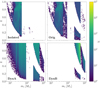Fig. 2

Distribution of the mass ratio q as a function of the primary mass m₁ for model log 1. We show the results for isolated, original (Orig), and dynamical (DynA and DynB) binaries in HM clusters. The color map shows the number of BBH mergers per cell.

3.6 Features in the mass ratio

Figure 6 shows the mass-ratio distribution for original and dynamical BBH mergers. Several features appear in the mass ratio of original BBHs, and they are markedly different for models labeled 1 (progenitor orbital period from Sana et al. 2012) and models labeled 5 (progenitor orbital period from Stacy & Bromm 2013).

In models assuming the initial orbital period from Stacy & Bromm (2013) (kro5, lar5, log5, and top5), we find

(i)
a peak at q ~ 0.15,
(ii)
a drop at q ~ 0.4,
(iii)
a steady increase for q > 0.4.

As already discussed in Sect. 3.3, the peak for q ~ 0.15 is mainly due to BBHs with m₁ above the upper-mass gap and m₂ below the gap. The peak is particularly evident in the case of the orbital periods from Stacy & Bromm (2013) because this set of initial conditions favors the formation of BBHs with low mass ratios (Costa et al. 2023). The majority of the BBH mergers with q ~ 0.15 in our simulations derive from binaries that did not undergo any type of mass transfer; these binaries did not merge within a Hubble time as isolated binaries (Costa et al. 2023). In original binaries, their merger is sped up by dynamical hardening.

In models assuming an initial orbital period from Sana et al. (2012) (kro1, lar1, log1, and top1), we find

(i)
a drop at q ≤ 0.4 (with an indication of a possible peak at 0.15 for models log1 and top1),
(ii)
a steady increase for q > 0.4,
(iii)
a peak at q ~ 0.8.

The peak at q ~ 0.8 for models assuming the Sana et al. (2012) orbital-period distribution is mainly due to BBHs with both m₁ and m₂ lower than ~100 M_⊙ (Sect. 3.3). As already discussed by Costa et al. (2023), these systems form through stable mass transfer; the mass ratio is low enough for the first mass transfer to occur while the secondary is still on the main sequence.

The central and right plot of Figure 6 show the mass-ratio distributions of dynamical BBHs using either the DynA or the DynB pairing criterion. We did not distinguish between models adopting Sana et al. (2012) or Stacy & Bromm (2013) because these BBHs form from stars that were initially single. The DynA and DynB models both have a strong preference for nearly equal-mass systems. However, they also show a peak at q ~ 0.15, corresponding to BBHs with a primary mass above the gap and a secondary mass below the gap. In models DynB, the drop at q below 0.4–0.5 is also steeper because these models yield a strong preference for mergers with both m₁ and m₂ above the mass gap (Fig. 1).

Fig. 3

Same as Figure 2, but with log1che.

Table 3

Final fate of original BBH mergers in HM clusters.

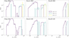Fig. 4

Distribution of the primary mass m₁ of BBH mergers for various generations in HM (top row) and LM clusters (bottom row). We show model log1.

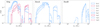Fig. 5

Primary mass distribution of BBH mergers for different initial conditions, defined in Table 1. The light blue (red) lines show initial conditions that assume the orbital period distribution by Sana et al. (2012) (Stacy & Bromm 2013) for the progenitor stars.

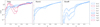Fig. 6

Mass-ratio distributions of BBH mergers for different initial conditions defined in Table 1. We show in light blue the initial conditions based on Sana et al. (2012), and we show in red the initial conditions based on Stacy & Bromm (2013).

Table 4

Final fate of dynamical BBH mergers (model DynA) in HM clusters.

Table 5

Final fate of dynamical BBH mergers (model DynB) in HM clusters.

4 Discussion

4.1 Survivability of globular clusters

We simulated our star clusters without taking the tidal field of their host galaxy into account. Hence, we do not know a priori when they become disrupted. We will include this calculation in a forthcoming study. Here, we wish to quantify how important our assumption is about the time at which the parent star cluster becomes disrupted. We therefore assumed that the star cluster is completely disrupted at redshift z_min = 10,6 and 2. In Figure D.1, we show that the mass distribution of BBH mergers does not vary for z_min < 10. The variation is <0.028% for log1 between z_min = 10 and z_min = 2.

The formation time of dynamical BBHs mainly depends on the dynamical friction timescale (Chandrasekhar 1943), $t_{DF} = \frac{3}{4 {(2 π)}^{1 / 2} G^{2} \ln Λ} \frac{σ^{3}}{m_{BH} ρ},$ ${t_{{\rm{DF}}}} = {3 \over {4{{(2\pi )}^{1/2}}{G^2}\ln \Lambda }}{{{\sigma ^3}} \over {{m_{{\rm{BH}}}}\rho }},$ (13)

where m_BH is the mass of the black hole that is segregated at the center of the cluster, ρ is the density at the half-mass radius, σ is the 3D velocity dispersion, and ln Λ is the Coulomb logarithm. The more massive the BH, the shorter the time it requires to sink to the center of the cluster and pair up with another BH. As a consequence, all the massive BHs in our clusters readily form a chain of mergers by z = 10.

Wang et al. (2022) recently hypothesized that the presence of a dark matter halo around the star cluster could protect it from tidal disruption and might in turn allow it to survive down to our redshift. However, because of the assumption of a top-heavy IMF for Pop. III stars, most of them evolve into BHs. Consequently, these clusters eventually evolve into dark clusters that are predominantly comprised of BH (Banerjee & Kroupa 2011), which makes them undetectable in the local Universe.

On the other hand, the uncertainties for the IMF of Pop. III stars and the current lack of observations of Pop. III star clusters in the local Universe lead to our assumption that the first star clusters were disrupted either during or shortly after the re-ionization epoch. The possibility that the clusters became disrupted at high redshift does not mean that we cannot observe Pop. III BBH mergers in the low-redshift Universe.

For a sense of what we can observe at low redshift with LIGO–Virgo–KAGRA, we continued to integrate our Pop. III BBHs down to redshift zero, assuming that they only evolve via GW decay after the disruption of their parent cluster. Fig. D.1 shows that the mass function of BBH mergers does not depend on the z_min of disruption of the cluster.

4.2 Merger rate density

Figure 7 shows the BBH merger rate density in HM and LM clusters. We only present our results for z_min = 10 because the mass distributions of BBH mergers do not vary at lower redshifts.

The merger rate density of dynamical BBHs (in HM and LM clusters) is higher than that of both original and isolated BBHs, especially at high redshift (z ≳ 5). Moreover, the merger rate density of dynamical BBHs peaks at z ~ 15 (earlier than the original and isolated BBHs) and then decreases rapidly. Most dynamical BBHs merge rapidly, with a short delay time. At later times, only the least massive BBH mergers remain. They are characterized by longer delay times.

In general, the merger rate density of BBHs in LM clusters is lower than that in HM clusters because the merger efficiency is lower (see Sect. 3.4). The LM clusters lose their black holes more efficiently than HM clusters.

Binary black holes that are born from CHE Pop. III stars yield a higher merger rate density in the case of isolated and original BBHs. This feature was already discussed in Santoliquido et al. (2023) and is due to the higher merger efficiency of CHE BBHs. The merger rate density of isolated BBHs also tends to be higher than that of original BBHs in star clusters because star-cluster dynamics tends to break some of the original binary stars, that is, those that are initially soft.

Figure 8 shows the merger rate density of BBHs with m₁ above the upper-mass gap. In model DynB, the merger rate density of BBHs with a primary mass above the gap is nearly the same as the total BBH merger rate density: nearly 100% BBHs are above the mass gap in model DynB.

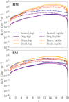Fig. 7

Merger rate density of Pop. III BBHs in star clusters. We assume that all of our clusters are disrupted at z_min = 10. We show both log1 (solid lines) and log1che (dashed lines). Isolated and original BBHs are shown in blue and purple, respectively. DynA and DynB BBHs are shown in red and orange, respectively. In the upper (lower) plot, we show the BBH merger rate density in HM (LM) clusters.

5 Summary

We have investigated the hierarchical mergers of Pop. III binary black holes (BBHs) in dense star clusters, exploring a wide range of initial conditions for the initial mass functions (IMFs) and formation channels of first-generation BBHs.

We find that the star-cluster dynamics boosts the merger rate of Pop. III BBHs with a mass above the pair-instability mass gap by several orders of magnitude. Our models predict that a dramatic difference between isolated and dynamical BBHs. Pop. III BBH mergers above the gap are rare in isolation (≲3%), while they are extremely common in dynamical BBHs. This difference is strongest with model DynB, which always yields ≳98% BBH mergers with a primary mass m₁ > 200 M_⊙.

Models with a chemically homogeneous evolution (CHE) show the least differences between isolated and dynamical BBHs above the gap because CHE favors the merger of isolated BBHs above the mass gap compared to default stellar evolution. Even in this case, however, the star-cluster dynamics allows the pair-up and merger of more massive BBHs and the formation of hierarchical chains that push m₁ up to ~700 M_⊙.

Our star cluster models predict several sharp features in the m₁ − q distribution of BBH mergers. We find a zone of avoidance in the m₁ − q plane, corresponding to the values for which either m₁ or m₂ are above the pair-instability mass gap. No such feature is apparent for isolated Pop. III BBH mergers because of the scarcity of mergers above the gap, unless we assume CHE.

The initial properties of the simulated star clusters affect the number of generations of mergers and the mass distributions. Because of their lower escape velocity, low-mass (LM) clusters host two generations of mergers at most and reach a maximum primary mass of ~1000 M_⊙. High-mass (HM) clusters instead host three generations of mergers at most and reach m₁ ~ 1200 M_⊙.

Different initial conditions result in peculiar features of the mass-ratio distribution of original BBHs. Models assuming initial orbital periods from Stacy & Bromm (2013) present a peak at q ~ 0.15. These BBHs do not merge within a Hubble time in isolation (Costa et al. 2023), while in star clusters their merger is triggered by dynamical hardening. Models assuming initial orbital periods from Sana et al. (2012) show a peak at q ~ 0.8, mainly due to BBHs that formed through stable mass transfer.

All our dynamical BBH models have a strong preference for nearly equal-mass systems. However, they also present a peak at q ~ 0.15, corresponding to BBHs with primary mass above the gap and secondary mass below the gap. The DynB models also predict a steep drop at q below 0.4–0.5 because of their strong preference for mergers with both m1 and m2 above the mass gap.

To take the effects of tidal disruption into account, we evolved our clusters up to a minimum redshift z_min . We showed that the m₁ − q distributions for z_min = 10, 6, 2 are almost identical. The most massive BBHs in the clusters merge by z = 10, while lower-mass BBHs are ejected by three-body interactions and merge outside the cluster by z = 0.

In HM clusters, the merger rate density of dynamical BBHs is generally higher than that of original and isolated BBHs: it peaks at z ∼ 15 and rapidly decreases at lower redshifts. We find a maximum value R(z = 15) ∼ 200 Gpc^-3 yr^-1 . At redshift zero, R(z = 0) ~ 0.32 Gpc⁻³ yr⁻¹ is still higher by a factor of ~ 13 than the one of isolated and original BBHs when we neglect CHE. The merger rate density of dynamical BBHs in LM clusters is lower than in HM clusters by up to one order of magnitude.

Isolated and original BBHs born from CHE Pop. III stars are also quite exceptional in terms of their merger rate. At redshift zero, it is similar to that of dynamical BBHs because these stars evolve with very compact radii and produce tight BBHs that merge more efficiently.

In summary, our results indicate that when Pop. III stars form and evolve in dense star clusters, dynamical interactions crucially enhance the formation of Pop. III BBH mergers above the pair-instability mass gap (≳200 M_⊙) compared to isolated binary evolution.

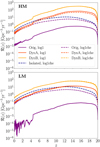Fig. 8

Same as Fig. 7,a but only for BBH mergers with primary mass above the pair-instability mass gap. Isolated Pop. III stars that do not evolve via CHE yield a merger rate density that is too low to be shown in the figure.

Acknowledgements

We thank the anonymous referee for their useful comments and suggestions, which helped us improve this manuscript. We thank Ralf Klessen, Veronika Lipatova, and Simon Glover for useful discussions. MM, ST, GC, GI, and FS acknowledge financial support from the European Research Council for the ERC Consolidator grant DEMOBLACK, under contract no. 770017. MM and ST also acknowledge financial support from the German Excellence Strategy via the Heidelberg Cluster of Excellence (EXC 2181 – 390900948) STRUCTURES. MB and MM also acknowledge support from the PRIN grant METE under the contract no. 2020KB33TP. FS acknowledges financial support from the AHEAD2020 project (grant agreement n. 871158). MAS acknowledges funding from the European Union’s Horizon 2020 research and innovation programme under the Marie Skłodowska-Curie grant agreement No. 101025436 (project GRACE-BH, PI: Manuel Arca Sedda). MAS acknowledges financial support from the MERAC Foundation. GC acknowledges financial support by the Agence Nationale de la Recherche grant POPSYCLE number ANR-19-CE31-0022. BM acknowledges funds from European Union – Next Generation EU.

Appendix A Initial conditions for Pop. III BBHs

In the following we describe the details of the initial conditions of our first-generation BHs, introduced in Sect. 2.1. We generated both the binary and single-star simulations with the population synthesis code SEVN (Iorio et al. 2023). We computed our star tracks using PARSEC, considering an initial mass range between 2 and 600 M_⊙ for default stars, and between 0.36 and 350 M⊙ for pure-He stars. We adopt the rapid model for supernova explosions (Fryer et al. 2012), which enforces a mass gap between neutron stars and BHs. For pulsational instability supernovae, we consider the prescription presented in the Appendix of Mapelli et al. (2020). For binary evolution, we assume a common envelope parameter α_CE = 1, while λ_CE is set self-consistently as in Claeys et al. (2014). Here we report the initial distribution for the primary mass, mass ratio, orbital period and eccentricity of original binaries. All the cases and combinations adopted in this work are listed in Table 1.

A.1 Original BBHs

Because of the lack of consensus on the IMF of Pop. III stars, we consider a range of IMFs for the primary mass:

(i)
A Kroupa (2001) IMF $ξ (M_{ZAMS}) \propto M_{ZAMS}^{- 2.3}$ $\xi \left( {{M_{{\rm{ZAMS}}}}} \right) \propto M_{{\rm{ZAMS}}}^{ - 2.3}$ , which is commonly adopted for Pop. II stars. With respect to the canonical IMF, here we consider a single slope since m_min ≥ 0.5M_⊙.
(ii)
A Larson (1998) IMF $ξ (M_{ZAMS}) \propto M_{ZAMS}^{- 2.35} \exp (- M_{cut 1} / M_{ZAMS})$ $\xi \left( {{M_{{\rm{ZAMS}}}}} \right) \propto M_{{\rm{ZAMS}}}^{ - 2.35}\exp \left( { - {M_{{\rm{cut}}1}}/{M_{{\rm{ZAMS}}}}} \right)$ , with M_cut1 = 20 M_⊙.
(iii)
A flat log distribution $ξ (M_{ZAMS}) \propto M_{ZAMS}^{- 1}$ $\xi \left( {{M_{{\rm{ZAMS}}}}} \right) \propto M_{{\rm{ZAMS}}}^{ - 1}$ (Stacy & Bromm 2013; Hirano et al. 2015; Susa et al. 2014; Wollen- berg et al. 2020; Chon et al. 2021; Tanikawa et al. 2021b; Jaura et al. 2022; Prole et al. 2022). We consider this IMF as the fiducial one in our work.
(iv)
A top heavy distribution (Stacy & Bromm 2013; Jaacks et al. 2019; Liu & Bromm 2020a), $ξ (M_{ZAMS}) \propto M_{ZAMS}^{- 0.17} \exp (- M_{cut 2}^{2} / M_{ZAMS}^{2})$ $\xi \left( {{M_{{\rm{ZAMS}}}}} \right) \propto M_{{\rm{ZAMS }}}^{ - 0.17}\exp \left( { - M_{{\rm{cut }}2}^2/M_{{\rm{ZAMS }}}^2} \right)$ , where M_cut2 = 20 M_⊙.

A.1.1 Mass ratio and secondary mass

We draw the secondary mass of the ZAMS star using three different prescriptions:

(i)
The q distribution from Sana et al. (2012), ξ(q) ∝ q^−0.1, with q ∈ [0.1, 1] and M_ZAMS,2 ≥ 2.2 M_⊙, which fits to the mass ratio of O- and B-type binaries in the local Universe.
(ii)
A sorted distribution: we draw the ZAMS mass of the entire stellar population from the chosen IMF. Then, we randomly pair two stars, enforcing M_ZAMS,2 ≤ M_ZAMS,1 .
(iii)
The q distribution from Stacy & Bromm (2013), ξ(q) ∝ q^−0.55, with q ∈ [0.1, 1] and M_ZAMS,2 ≥ 2.2 M_⊙. This distribution was obtained by fitting Pop. III stars generated in cosmological simulations.

A.1.2 Orbital period

We adopt two distributions for the initial orbital period P.

(i)
ξ(Π) ∝ Π⁻⁰·⁵⁵, with Π = log (P/day) ∈ [0.15, 5.5] from Sana et al. (2012).
(ii)
ξ(Π) ∝ exp [− (Π − µ)² / (2σ²)], that is a Gaussian distribution with µ = 5.5 and σ = 0.85 (Stacy & Bromm 2013).

A.1.3 Eccentricity

We draw the orbital eccentricity e from two distributions.

(i)
ξ(e) ∝ e^−0.42 with e ∈ [0, 1) (Sana et al. 2012).
(ii)
A thermal distribution ξ(e) = 2e with e ∈ [0,1) (Heggie 1975; Tanikawa et al. 2021b; Hartwig et al. 2016; Kinugawa et al. 2014), which favors highly eccentric systems. As shown by Park et al. (2021, 2023), Pop. III binaries form preferentially with high orbital eccentricity.

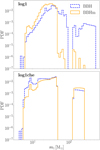Fig. A.1

Distribution of BBHs (blue dashed line) and BBH mergers (orange solid line) from isolated binary star progenitors (Costa et al. 2023; Santoliquido et al. 2023). We show the log1 (upper panel) and log1che (lower panel) models.

A.2 Chemically-homogeneous stars

In this work, we model CHE from pure-He stars, following San- toliquido et al. (2023). Fast-spinning metal-poor stars effectively become fully mixed by the end of the main sequence (Mandel & de Mink 2016; de Mink & Mandel 2016). For this reason, pure-He stars can be used to describe the successive phases of their evolution (Tanikawa et al. 2021a). In our treatment, we use pure-He stars as a proxy for CHE after the main sequence (Santoliquido et al. 2023). To account for the hydrogen burning phase, we assume that the evolution of pure-He stars starts at the end of the main sequence in our dynamical simulations with FASTCLUSTER.

CHE stars remain pretty compact during their entire evolution (Tanikawa et al. 2021b). This generally prevents Pop. III chemically-homogeneous stars from merging in the early stages of their life. Figure A.1 compares the distributions of isolated Pop. III BBHs and BBH mergers from models log1 and log1che (Costa et al. 2023; Santoliquido et al. 2023). Isolated BBH mergers with primary mass m₁ > 10² M_⊙ are extremely rare, because their stellar progenitors merge with their companion when they become giant stars. In contrast, CHE stars evolve with compact radii for their entire life, thus preventing the BH progenitors from becoming giant stars at the end of the main sequence. As a consequence, CHE binaries can efficiently produce BBH mergers above the upper mass gap.

Appendix B Pairing functions

We draw the masses of our dynamical BBHs from catalogs of single BHs obtained with SEVN (Iorio et al. 2023). We consider the same initial conditions as for original binaries (Sect. A.1). Since the P and e distributions are set based on dynamical prescriptions (eq. 1), we only draw the BH mass from the SEVN catalogs. Thus, the only parameters of interest for dynamical BBHs in Table 1 are M_ZAMS,₁, N and M_tot. We draw these parameters from the models kro1, lar1, log1 and top1.

We consider two different coupling criteria for generating the first-generation dynamical BBH masses. In model DynA, we sample the mass of the primary BH uniformly from the SEVN single BH catalog (Mapelli et al. 2021), while the secondary is drawn from the probability distribution function (O’Leary et al. 2016): $p (m_{2}) \propto {(m_{1} + m_{2})}^{4} with m_{2} \in [5 M_{⊙}, m_{1}) .$ $p\left( {{m_2}} \right) \propto {\left( {{m_1} + {m_2}} \right)^4}\quad {\rm{with}}{m_2} \in \left[ {5{{\rm{M}}_ \odot },{m_1}} \right){\rm{.}}$ (B.1)

In model DynB, we derive the primary and secondary BH masses following the sampling criterion introduced in Antonini et al. (2023), which is based on the formation rate of hard binaries per unit of volume and energy Heggie (1975): $Γ_{3 b} (m_{1}, m_{2}, m_{3}) \propto \frac{n_{1} n_{2} n_{3} m_{1}^{4} m_{2}^{4} m_{3}^{5 / 2}}{{(m_{1} + m_{2} + m_{3})}^{1 / 2} {(m_{1} + m_{2})}^{1 / 2}} β^{9 / 2},$ ${\Gamma _{3{\rm{b}}}}\left( {{m_1},{m_2},{m_3}} \right) \propto {{{n_1}{n_2}{n_3}m_1^4m_2^4m_3^{5/2}} \over {{{\left( {{m_1} + {m_2} + {m_3}} \right)}^{1/2}}{{\left( {{m_1} + {m_2}} \right)}^{1/2}}}}{\beta ^{9/2}},$ (B.2)

with n_i = n(m_i) the number density of BHs with mass mi (i =1,2,3) and β the inverse of their mean internal energy. For each model, we derive n(m) from the mass function of single BHs in the SEVN catalog. Since eq. B.2 is symmetric in m1 and m2, the probability density function for either of them is $p_{1, 2} (m_{1, 2}) = \int_{m_{low}}^{m_{up}} \int_{m_{low}}^{m_{up}} d m_{3} d m_{2, 1} Γ_{3 b} (m_{1}, m_{2}, m_{3}),$ ${p_{1,2}}\left( {{m_{1,2}}} \right) = \int_{{m_{{\rm{low}}}}}^{{m_{{\rm{up}}}}} {\int_{{m_{{\rm{low}}}}}^{{m_{{\rm{up}}}}} {d{m_3}} } d{m_{2,1}}{\Gamma _{3{\rm{b}}}}\left( {{m_1},{m_2},{m_3}} \right),$ (B.3)

where m_low and m_up are the lower and upper limit of the mass distribution. Using eq. B.3, we sample the primary and secondary mass of the BBHs and then we assign the largest one to m₁ and the smallest to m2 . As shown in Fig. B.1, the model DynA tends to reproduce the underlying BH mass function, while DynB favors the coupling of the most massive BHs.

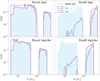Fig. B.1

Distribution of m₁ (purple solid line) and m₂ (violet dashed line) for first-generation BBHs, for model DynA (left) and DynB (right). The blue shaded area represents the distribution of single BHs from the SEVN catalog. We show the log1 (upper panel) and log1che (lower panel) models.

Appendix C Uncertainties related to stochastic fluctuations on model DynB

The sampling criterion in model DynB strongly favors the coupling of the most massive BHs, as expected from dynamical interactions in high-density star clusters (Heggie 1975). However, only a limited number of BHs may be present in a single star cluster, and in particular in those with M_cl ≲ 10⁴ M_⊙.

Here, we quantify the effect of stochastic fluctuations due to the limited number of BHs in a star cluster on the BBH mergers predicted by model DynB. First, we define the formation rate of hard binaries per unit of volume and energy (eq. B.2), as described in Appendix B. Then, we randomly draw a sub-sample with size N from the SEVN catalog, to mimic the presence of a certain number of BHs within the cluster. Finally, we sample the BH masses from this set, instead of the whole SEVN catalog, based on the probability density function defined in eq. B.3.

Figure C.1 shows the primary and secondary BH masses in BBH mergers, obtained by considering N = 10 and 100 BHs for model log1. The BH distributions for N = 100 are almost identical to the case without restrictions, because the sub-samples are large enough to contain a number of massive BHs, which are most likely coupled in our model. In contrast, when N = 10 the very limited number of BHs allow for the coupling of less massive BHs, with primary mass m₁ ≲ 100 M_⊙ . As a consequence, the primary mass distribution of BBH mergers now extends below the pair-instability mass gap, down to ∼20 M_⊙ .

Appendix D Impact of cluster survivability

As discussed in Sec. 4.1, we simulated the evolution of our clusters up to a minimum redshift z_min, with z_min = 2, 6 and 10 and evaluate the impact of z_min on the number of BBH mergers. In the following, we account for the effects of tidal disruption on the number and mass distributions of BBH mergers.

We find negligible difference in the populations of BBH mergers at different z_min . Table D.1 reports the percentage variation of the number of BBH mergers between z_min = 10 and z_min = 2. Such variation is always smaller than 0.05%. Fig. D.1 shows the distributions of BBH mergers in the m₁ − q plane, for different z_min . Independently of the model considered, there are minimal differences between the mass spectra of BBH mergers at z_min ≤ 10.

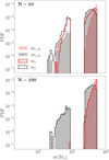Fig. C.1

Distribution of m₁ (red solid line) and m₂ (black dashed line) for BBH mergers with model DynB in HM clusters. We obtain them considering, at each drawing, sub-samples of the SEVN catalog with size 10 (upper panel) and 100 (lower panel), respectively. The shaded areas show the distributions obtained when sampling the 1g BHs from the SEVN catalog without any restriction.

Table D.1

BBH mergers at z_min = 10 vs. z_min = 2

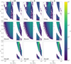Fig. D.1

Distribution of the mass ratio q as a function of the primary mass m1 for model log1, assuming that the HM cluster gets disrupted at redshift zmin = 10, 6, 2. We show the results both for original (Orig) and dynamical (DynA and DynB) binaries.

References

Abbott, B. P., et al. (LIGO Scientific Collaboration, Virgo Collaboration, and KAGRA Collaboration) 2020, Living Rev. Relativ., 23, 3 [NASA ADS] [CrossRef] [Google Scholar]
Abbott, R., et al. (LIGO Scientific Collaboration, Virgo Collaboration, and KAGRA Collaboration) 2023a, Phys. Rev. X, 13, 041039 [Google Scholar]
Abbott, R., et al. (LIGO Scientific Collaboration, Virgo Collaboration, and KAGRA Collaboration) 2023b, Phys. Rev. X, 13, 011048 [NASA ADS] [Google Scholar]
Abbott, R., et al. (LIGO Scientific Collaboration, Virgo Collaboration, and KAGRA Collaboration) 2023c, Phys. Rev. X, 13, 011048 [NASA ADS] [Google Scholar]
Antonini, F., & Gieles, M. 2020, MNRAS, 492, 2936 [CrossRef] [Google Scholar]
Antonini, F., Gieles, M., Dosopoulou, F., & Chattopadhyay, D. 2023, MNRAS, 522, 466 [NASA ADS] [CrossRef] [Google Scholar]
Baibhav, V., Gerosa, D., Berti, E., et al. 2020, Phys. Rev. D, 102, 043002 [NASA ADS] [CrossRef] [Google Scholar]
Banerjee, S., & Kroupa, P. 2011, ApJ, 741, L12 [NASA ADS] [CrossRef] [Google Scholar]
Belczynski, K., Holz, D. E., Bulik, T., & O’Shaughnessy, R. 2016, Nature, 534, 512 [NASA ADS] [CrossRef] [Google Scholar]
Belczynski, K., Ryu, T., Perna, R., et al. 2017, MNRAS, 471, 4702 [Google Scholar]
Branchesi, M., Maggiore, M., Alonso, D., et al. 2023, J. Cosmology Astropart. Phys., 2023, 068 [CrossRef] [Google Scholar]
Bressan, A., Marigo, P., Girardi, L., et al. 2012, MNRAS, 427, 127 [NASA ADS] [CrossRef] [Google Scholar]
Bromm, V., & Clarke, C. J. 2002, ApJ, 566, L1 [NASA ADS] [CrossRef] [Google Scholar]
Carr, B., Kühnel, F., & Sandstad, M. 2016, Phys. Rev. D, 94, 083504 [CrossRef] [Google Scholar]
Chandrasekhar, S. 1943, ApJ, 97, 255 [Google Scholar]
Chen, Y., Bressan, A., Girardi, L., et al. 2015, MNRAS, 452, 1068 [Google Scholar]
Chon, S., Omukai, K., & Schneider, R. 2021, MNRAS, 508, 4175 [NASA ADS] [CrossRef] [Google Scholar]
Claeys, J. S. W., Pols, O. R., Izzard, R. G., Vink, J., & Verbunt, F. W. M. 2014, A&A, 563, A83 [NASA ADS] [CrossRef] [EDP Sciences] [Google Scholar]
Costa, G., Girardi, L., Bressan, A., et al. 2019, MNRAS, 485, 4641 [NASA ADS] [CrossRef] [Google Scholar]
Costa, G., Bressan, A., Mapelli, M., et al. 2021, MNRAS, 501, 4514 [NASA ADS] [CrossRef] [Google Scholar]
Costa, G., Mapelli, M., Iorio, G., et al. 2023, MNRAS, 525, 2891 [NASA ADS] [CrossRef] [Google Scholar]
de Mink, S. E., & Mandel, I. 2016, MNRAS, 460, 3545 [NASA ADS] [CrossRef] [Google Scholar]
Fryer, C. L., Belczynski, K., Wiktorowicz, G., et al. 2012, ApJ, 749, 91 [Google Scholar]
Georgiev, I. Y., Puzia, T. H., Hilker, M., & Goudfrooij, P. 2009, MNRAS, 392, 879 [NASA ADS] [CrossRef] [Google Scholar]
Goodman, J., & Hut, P. 1989, Nature, 339, 40 [NASA ADS] [CrossRef] [Google Scholar]
Haiman, Z., Thoul, A. A., & Loeb, A. 1996, ApJ, 464, 523 [NASA ADS] [CrossRef] [Google Scholar]
Hartwig, T., Volonteri, M., Bromm, V., et al. 2016, MNRAS, 460, L74 [NASA ADS] [CrossRef] [Google Scholar]
Hartwig, T., Magg, M., Chen, L.-H., et al. 2022, ApJ, 936, 45 [NASA ADS] [CrossRef] [Google Scholar]
He, C.-C., Ricotti, M., & Geen, S. 2019, MNRAS, 489, 1880 [NASA ADS] [CrossRef] [Google Scholar]
Heger, A., Woosley, S., Baraffe, I., & Abel, T. 2002, in Lighthouses of the Universe: The Most Luminous Celestial Objects and Their Use for Cosmology, eds. M. Gilfanov, R. Sunyeav, & E. Churazov, 369 [Google Scholar]
Heggie, D. C. 1975, MNRAS, 173, 729 [NASA ADS] [CrossRef] [Google Scholar]
Hills, J. G. 1983, AJ, 88, 1269 [NASA ADS] [CrossRef] [Google Scholar]
Hirano, S., Hosokawa, T., Yoshida, N., Omukai, K., & Yorke, H. W. 2015, MNRAS, 448, 568 [NASA ADS] [CrossRef] [Google Scholar]
Hurley, J. R., Tout, C. A., & Pols, O. R. 2002, MNRAS, 329, 897 [Google Scholar]
Iorio, G., Mapelli, M., Costa, G., et al. 2023, MNRAS, 524, 426 [NASA ADS] [CrossRef] [Google Scholar]
Jaacks, J., Finkelstein, S. L., & Bromm, V. 2019, MNRAS, 488, 2202 [NASA ADS] [CrossRef] [Google Scholar]
Jaura, O., Glover, S. C. O., Wollenberg, K. M. J., et al. 2022, MNRAS, 512, 116 [NASA ADS] [CrossRef] [Google Scholar]
Jiménez-Forteza, X., Keitel, D., Husa, S., et al. 2017, Phys. Rev. D, 95, 064024 [CrossRef] [Google Scholar]
Kalogera, V., Sathyaprakash, B. S., Bailes, M., et al. 2021, arXiv e-prints [arXiv: 2111.06990] [Google Scholar]
Kinugawa, T., Inayoshi, K., Hotokezaka, K., Nakauchi, D., & Nakamura, T. 2014, MNRAS, 442, 2963 [NASA ADS] [CrossRef] [Google Scholar]
Kinugawa, T., Miyamoto, A., Kanda, N., & Nakamura, T. 2016, MNRAS, 456, 1093 [CrossRef] [Google Scholar]
Kinugawa, T., Nakamura, T., & Nakano, H. 2021, MNRAS, 501, L49 [Google Scholar]
Klessen, R. S., & Glover, S. C. O. 2023, ARA&A, 61, 65 [NASA ADS] [CrossRef] [Google Scholar]
Komatsu, E., Smith, K. M., Dunkley, J., et al. 2011, ApJS, 192, 18 [Google Scholar]
Kroupa, P. 2001, MNRAS, 322, 231 [NASA ADS] [CrossRef] [Google Scholar]
Larson, R. B. 1998, MNRAS, 301, 569 [NASA ADS] [CrossRef] [Google Scholar]
Liu, B., & Bromm, V. 2020a, MNRAS, 495, 2475 [NASA ADS] [CrossRef] [Google Scholar]
Liu, B., & Bromm, V. 2020b, ApJ, 903, L40 [NASA ADS] [CrossRef] [Google Scholar]
Lousto, C. O., Zlochower, Y., Dotti, M., & Volonteri, M. 2012, Phys. Rev. D, 85, 084015 [NASA ADS] [CrossRef] [Google Scholar]
Madau, P., & Rees, M. J. 2001, ApJ, 551, L27 [Google Scholar]
Maeder, A. 1987, A&A, 178, 159 [NASA ADS] [Google Scholar]
Mandel, I., & de Mink, S. E. 2016, MNRAS, 458, 2634 [NASA ADS] [CrossRef] [Google Scholar]
Mapelli, M., Spera, M., Montanari, E., et al. 2020, ApJ, 888, 76 [NASA ADS] [CrossRef] [Google Scholar]
Mapelli, M., Dall’Amico, M., Bouffanais, Y., et al. 2021, MNRAS, 505, 339 [CrossRef] [Google Scholar]
Mapelli, M., Bouffanais, Y., Santoliquido, F., Arca Sedda, M., & Artale, M. C. 2022, MNRAS, 511, 5797 [NASA ADS] [CrossRef] [Google Scholar]
Marchant, P., Langer, N., Podsiadlowski, P., Tauris, T. M., & Moriya, T. J. 2016, A&A, 588, A50 [NASA ADS] [CrossRef] [EDP Sciences] [Google Scholar]
Miller, M. C., & Colbert, E. J. M. 2004, Int. J. Mod. Phys. D, 13, 1 [NASA ADS] [CrossRef] [Google Scholar]
Miller, M. C., & Hamilton, D. P. 2002, MNRAS, 330, 232 [Google Scholar]
Ng, K. K. Y., Vitale, S., Farr, W. M., & Rodriguez, C. L. 2021, ApJ, 913, L5 [NASA ADS] [CrossRef] [Google Scholar]
Ng, K. K. Y., Chen, S., Goncharov, B., et al. 2022a, ApJ, 931, L12 [NASA ADS] [CrossRef] [Google Scholar]
Ng, K. K. Y., Franciolini, G., Berti, E., et al. 2022b, ApJ, 933, L41 [NASA ADS] [CrossRef] [Google Scholar]
O’Leary, R. M., Meiron, Y., & Kocsis, B. 2016, ApJ, 824, L12 [CrossRef] [Google Scholar]
Özel, F. & Freire, P. 2016, ARA&A, 54, 401 [CrossRef] [Google Scholar]
Park, J., Ricotti, M., & Sugimura, K. 2021, MNRAS, 508, 6193 [NASA ADS] [CrossRef] [Google Scholar]
Park, J., Ricotti, M., & Sugimura, K. 2023, MNRAS, 521, 5334 [NASA ADS] [CrossRef] [Google Scholar]
Périgois, C., Belczynski, C., Bulik, T., & Regimbau, T. 2021, Phys. Rev. D, 103, 043002 [CrossRef] [Google Scholar]
Peters, P. C. 1964, Phys. Rev., 136, 1224 [Google Scholar]
Planck Collaboration VI. 2020, A&A, 641, A6 [NASA ADS] [CrossRef] [EDP Sciences] [Google Scholar]
Prole, L. R., Clark, P. C., Klessen, R. S., & Glover, S. C. O. 2022, MNRAS, 510, 4019 [NASA ADS] [CrossRef] [Google Scholar]
Punturo, M., Abernathy, M., Acernese, F., et al. 2010, Class. Quant. Grav., 27, 194002 [Google Scholar]
Quinlan, G. D. 1996, New A, 1, 35 [NASA ADS] [CrossRef] [Google Scholar]
Reed, D. S., Bower, R., Frenk, C. S., Jenkins, A., & Theuns, T. 2007, MNRAS, 374, 2 [NASA ADS] [CrossRef] [Google Scholar]
Reitze, D., Adhikari, R. X., Ballmer, S., et al. 2019, Bull. Am. Astron. Soc., 51, 35 [Google Scholar]
Riley, J., Agrawal, P., Barrett, J. W., et al. 2022, ApJS, 258, 34 [NASA ADS] [CrossRef] [Google Scholar]
Rodriguez, C. L., Zevin, M., Pankow, C., Kalogera, V., & Rasio, F. A. 2016, ApJ, 832, L2 [NASA ADS] [CrossRef] [Google Scholar]
Sakurai, Y., Yoshida, N., Fujii, M. S., & Hirano, S. 2017, MNRAS, 472, 1677 [NASA ADS] [CrossRef] [Google Scholar]
Sana, H., de Mink, S. E., de Koter, A., et al. 2012, Science, 337, 444 [Google Scholar]
Santoliquido, F., Mapelli, M., Bouffanais, Y., et al. 2020, ApJ, 898, 152 [Google Scholar]
Santoliquido, F., Mapelli, M., Giacobbo, N., Bouffanais, Y., & Artale, M. C. 2021, MNRAS, 502, 4877 [NASA ADS] [CrossRef] [Google Scholar]
Santoliquido, F., Mapelli, M., Iorio, G., et al. 2023, MNRAS, 524, 307 [NASA ADS] [CrossRef] [Google Scholar]
Santoliquido, F., Dupletsa, U., Tissino, J., et al. 2024, A&A, in press, https://doi.org/18.1851/8884-6361/282458381 [NASA ADS] [CrossRef] [EDP Sciences] [Google Scholar]
Sesana, A., Haardt, F., & Madau, P. 2006, ApJ, 651, 392 [Google Scholar]
Sharda, P., Federrath, C., & Krumholz, M. R. 2020, MNRAS, 497, 336 [NASA ADS] [CrossRef] [Google Scholar]
Spera, M., Mapelli, M., Giacobbo, N., et al. 2019, MNRAS, 485, 889 [Google Scholar]
Stacy, A., & Bromm, V. 2013, MNRAS, 433, 1094 [NASA ADS] [CrossRef] [Google Scholar]
Susa, H., Hasegawa, K., & Tominaga, N. 2014, ApJ, 792, 32 [NASA ADS] [CrossRef] [Google Scholar]
Tanikawa, A. 2024, Rev. Mod. Plasma Phys., 8, 13 [NASA ADS] [CrossRef] [Google Scholar]
Tanikawa, A., Kinugawa, T., Yoshida, T., Hijikawa, K., & Umeda, H. 2021a, MNRAS, 505, 2170 [CrossRef] [Google Scholar]
Tanikawa, A., Susa, H., Yoshida, T., Trani, A. A., & Kinugawa, T. 2021b, ApJ, 910, 30 [NASA ADS] [CrossRef] [Google Scholar]
Tanikawa, A., Yoshida, T., Kinugawa, T., et al. 2022, ApJ, 926, 83 [NASA ADS] [CrossRef] [Google Scholar]
Tanikawa, A., Moriya, T. J., Tominaga, N., & Yoshida, N. 2023, MNRAS, 519, L32 [Google Scholar]
Tegmark, M., Silk, J., Rees, M. J., et al. 1997, ApJ, 474, 1 [NASA ADS] [CrossRef] [Google Scholar]
Torniamenti, S., Mapelli, M., Périgois, C., et al. 2024, A&A, 688, A148 [NASA ADS] [CrossRef] [EDP Sciences] [Google Scholar]
Vaccaro, M. P., Mapelli, M., Périgois, C., et al. 2024, A&A, 685, A51 [NASA ADS] [CrossRef] [EDP Sciences] [Google Scholar]
Wang, L., Tanikawa, A., & Fujii, M. 2022, MNRAS, 515, 5106 [NASA ADS] [CrossRef] [Google Scholar]
Wollenberg, K. M. J., Glover, S. C. O., Clark, P. C., & Klessen, R. S. 2020, MNRAS, 494, 1871 [NASA ADS] [CrossRef] [Google Scholar]
Woosley, S. E., & Heger, A. 2006, ApJ, 637, 914 [CrossRef] [Google Scholar]
Woosley, S. E., Heger, A., & Weaver, T. A. 2002, Rev. Mod. Phys., 74, 1015 [NASA ADS] [CrossRef] [Google Scholar]
Yoshida, N., Abel, T., Hernquist, L., & Sugiyama, N. 2003, ApJ, 592, 645 [CrossRef] [Google Scholar]

All Tables

Table 1

Initial conditions for the stellar models.

In the text

Table 2

Binary black hole mergers above the upper-mass gap.

In the text

Table 3

Final fate of original BBH mergers in HM clusters.

In the text

Table 4

Final fate of dynamical BBH mergers (model DynA) in HM clusters.

In the text

Table 5

Final fate of dynamical BBH mergers (model DynB) in HM clusters.

In the text

Table D.1

BBH mergers at z_min = 10 vs. z_min = 2

In the text

All Figures

	Fig. 1 Distributions of primary (red) and secondary (black) masses of BBHs merging in HM clusters for log1 (upper panels) and log1che (lower panels). The shaded histograms show the results found by Costa et al. (2023) for isolated BBHs. The left column shows the results found with the pairing function DynA, and the right column shows the results with DynB.
In the text

	Fig. 2 Distribution of the mass ratio q as a function of the primary mass m₁ for model log 1. We show the results for isolated, original (Orig), and dynamical (DynA and DynB) binaries in HM clusters. The color map shows the number of BBH mergers per cell.
In the text

	Fig. 3 Same as Figure 2, but with log1che.
In the text

	Fig. 4 Distribution of the primary mass m₁ of BBH mergers for various generations in HM (top row) and LM clusters (bottom row). We show model log1.
In the text

	Fig. 5 Primary mass distribution of BBH mergers for different initial conditions, defined in Table 1. The light blue (red) lines show initial conditions that assume the orbital period distribution by Sana et al. (2012) (Stacy & Bromm 2013) for the progenitor stars.
In the text

	Fig. 6 Mass-ratio distributions of BBH mergers for different initial conditions defined in Table 1. We show in light blue the initial conditions based on Sana et al. (2012), and we show in red the initial conditions based on Stacy & Bromm (2013).
In the text

Fig. 7

Merger rate density of Pop. III BBHs in star clusters. We assume that all of our clusters are disrupted at z_min = 10. We show both log1 (solid lines) and log1che (dashed lines). Isolated and original BBHs are shown in blue and purple, respectively. DynA and DynB BBHs are shown in red and orange, respectively. In the upper (lower) plot, we show the BBH merger rate density in HM (LM) clusters.

In the text

	Fig. 8 Same as Fig. 7,a but only for BBH mergers with primary mass above the pair-instability mass gap. Isolated Pop. III stars that do not evolve via CHE yield a merger rate density that is too low to be shown in the figure.
In the text

	Fig. A.1 Distribution of BBHs (blue dashed line) and BBH mergers (orange solid line) from isolated binary star progenitors (Costa et al. 2023; Santoliquido et al. 2023). We show the log1 (upper panel) and log1che (lower panel) models.
In the text

	Fig. B.1 Distribution of m₁ (purple solid line) and m₂ (violet dashed line) for first-generation BBHs, for model DynA (left) and DynB (right). The blue shaded area represents the distribution of single BHs from the SEVN catalog. We show the log1 (upper panel) and log1che (lower panel) models.
In the text

	Fig. C.1 Distribution of m₁ (red solid line) and m₂ (black dashed line) for BBH mergers with model DynB in HM clusters. We obtain them considering, at each drawing, sub-samples of the SEVN catalog with size 10 (upper panel) and 100 (lower panel), respectively. The shaded areas show the distributions obtained when sampling the 1g BHs from the SEVN catalog without any restriction.
In the text

	Fig. D.1 Distribution of the mass ratio q as a function of the primary mass m1 for model log1, assuming that the HM cluster gets disrupted at redshift zmin = 10, 6, 2. We show the results both for original (Orig) and dynamical (DynA and DynB) binaries.
In the text

Current usage metrics show cumulative count of Article Views (full-text article views including HTML views, PDF and ePub downloads, according to the available data) and Abstracts Views on Vision4Press platform.

Data correspond to usage on the plateform after 2015. The current usage metrics is available 48-96 hours after online publication and is updated daily on week days.

Initial download of the metrics may take a while.

[1] Abbott, B. P., et al. (LIGO Scientific Collaboration, Virgo Collaboration, and KAGRA Collaboration) 2020, Living Rev. Relativ., 23, 3 [NASA ADS] [CrossRef] [Google Scholar]

[2] Abbott, R., et al. (LIGO Scientific Collaboration, Virgo Collaboration, and KAGRA Collaboration) 2023a, Phys. Rev. X, 13, 041039 [Google Scholar]

[3] Abbott, R., et al. (LIGO Scientific Collaboration, Virgo Collaboration, and KAGRA Collaboration) 2023b, Phys. Rev. X, 13, 011048 [NASA ADS] [Google Scholar]

[4] Abbott, R., et al. (LIGO Scientific Collaboration, Virgo Collaboration, and KAGRA Collaboration) 2023c, Phys. Rev. X, 13, 011048 [NASA ADS] [Google Scholar]

[5] Antonini, F., & Gieles, M. 2020, MNRAS, 492, 2936 [CrossRef] [Google Scholar]

[6] Antonini, F., Gieles, M., Dosopoulou, F., & Chattopadhyay, D. 2023, MNRAS, 522, 466 [NASA ADS] [CrossRef] [Google Scholar]

[7] Baibhav, V., Gerosa, D., Berti, E., et al. 2020, Phys. Rev. D, 102, 043002 [NASA ADS] [CrossRef] [Google Scholar]

[8] Banerjee, S., & Kroupa, P. 2011, ApJ, 741, L12 [NASA ADS] [CrossRef] [Google Scholar]

[9] Belczynski, K., Holz, D. E., Bulik, T., & O’Shaughnessy, R. 2016, Nature, 534, 512 [NASA ADS] [CrossRef] [Google Scholar]

[10] Belczynski, K., Ryu, T., Perna, R., et al. 2017, MNRAS, 471, 4702 [Google Scholar]

[11] Branchesi, M., Maggiore, M., Alonso, D., et al. 2023, J. Cosmology Astropart. Phys., 2023, 068 [CrossRef] [Google Scholar]

[12] Bressan, A., Marigo, P., Girardi, L., et al. 2012, MNRAS, 427, 127 [NASA ADS] [CrossRef] [Google Scholar]

[13] Bromm, V., & Clarke, C. J. 2002, ApJ, 566, L1 [NASA ADS] [CrossRef] [Google Scholar]

[14] Carr, B., Kühnel, F., & Sandstad, M. 2016, Phys. Rev. D, 94, 083504 [CrossRef] [Google Scholar]

[15] Chandrasekhar, S. 1943, ApJ, 97, 255 [Google Scholar]

[16] Chen, Y., Bressan, A., Girardi, L., et al. 2015, MNRAS, 452, 1068 [Google Scholar]

[17] Chon, S., Omukai, K., & Schneider, R. 2021, MNRAS, 508, 4175 [NASA ADS] [CrossRef] [Google Scholar]

[18] Claeys, J. S. W., Pols, O. R., Izzard, R. G., Vink, J., & Verbunt, F. W. M. 2014, A&A, 563, A83 [NASA ADS] [CrossRef] [EDP Sciences] [Google Scholar]

[19] Costa, G., Girardi, L., Bressan, A., et al. 2019, MNRAS, 485, 4641 [NASA ADS] [CrossRef] [Google Scholar]

[20] Costa, G., Bressan, A., Mapelli, M., et al. 2021, MNRAS, 501, 4514 [NASA ADS] [CrossRef] [Google Scholar]

[21] Costa, G., Mapelli, M., Iorio, G., et al. 2023, MNRAS, 525, 2891 [NASA ADS] [CrossRef] [Google Scholar]

[22] de Mink, S. E., & Mandel, I. 2016, MNRAS, 460, 3545 [NASA ADS] [CrossRef] [Google Scholar]

[23] Fryer, C. L., Belczynski, K., Wiktorowicz, G., et al. 2012, ApJ, 749, 91 [Google Scholar]

[24] Georgiev, I. Y., Puzia, T. H., Hilker, M., & Goudfrooij, P. 2009, MNRAS, 392, 879 [NASA ADS] [CrossRef] [Google Scholar]

[25] Goodman, J., & Hut, P. 1989, Nature, 339, 40 [NASA ADS] [CrossRef] [Google Scholar]

[26] Haiman, Z., Thoul, A. A., & Loeb, A. 1996, ApJ, 464, 523 [NASA ADS] [CrossRef] [Google Scholar]

[27] Hartwig, T., Volonteri, M., Bromm, V., et al. 2016, MNRAS, 460, L74 [NASA ADS] [CrossRef] [Google Scholar]

[28] Hartwig, T., Magg, M., Chen, L.-H., et al. 2022, ApJ, 936, 45 [NASA ADS] [CrossRef] [Google Scholar]

[29] He, C.-C., Ricotti, M., & Geen, S. 2019, MNRAS, 489, 1880 [NASA ADS] [CrossRef] [Google Scholar]

[30] Heger, A., Woosley, S., Baraffe, I., & Abel, T. 2002, in Lighthouses of the Universe: The Most Luminous Celestial Objects and Their Use for Cosmology, eds. M. Gilfanov, R. Sunyeav, & E. Churazov, 369 [Google Scholar]

[31] Heggie, D. C. 1975, MNRAS, 173, 729 [NASA ADS] [CrossRef] [Google Scholar]

[32] Hills, J. G. 1983, AJ, 88, 1269 [NASA ADS] [CrossRef] [Google Scholar]

[33] Hirano, S., Hosokawa, T., Yoshida, N., Omukai, K., & Yorke, H. W. 2015, MNRAS, 448, 568 [NASA ADS] [CrossRef] [Google Scholar]

[34] Hurley, J. R., Tout, C. A., & Pols, O. R. 2002, MNRAS, 329, 897 [Google Scholar]

[35] Iorio, G., Mapelli, M., Costa, G., et al. 2023, MNRAS, 524, 426 [NASA ADS] [CrossRef] [Google Scholar]

[36] Jaacks, J., Finkelstein, S. L., & Bromm, V. 2019, MNRAS, 488, 2202 [NASA ADS] [CrossRef] [Google Scholar]

[37] Jaura, O., Glover, S. C. O., Wollenberg, K. M. J., et al. 2022, MNRAS, 512, 116 [NASA ADS] [CrossRef] [Google Scholar]

[38] Jiménez-Forteza, X., Keitel, D., Husa, S., et al. 2017, Phys. Rev. D, 95, 064024 [CrossRef] [Google Scholar]

[39] Kalogera, V., Sathyaprakash, B. S., Bailes, M., et al. 2021, arXiv e-prints [arXiv: 2111.06990] [Google Scholar]

[40] Kinugawa, T., Inayoshi, K., Hotokezaka, K., Nakauchi, D., & Nakamura, T. 2014, MNRAS, 442, 2963 [NASA ADS] [CrossRef] [Google Scholar]

[41] Kinugawa, T., Miyamoto, A., Kanda, N., & Nakamura, T. 2016, MNRAS, 456, 1093 [CrossRef] [Google Scholar]

[42] Kinugawa, T., Nakamura, T., & Nakano, H. 2021, MNRAS, 501, L49 [Google Scholar]

[43] Klessen, R. S., & Glover, S. C. O. 2023, ARA&A, 61, 65 [NASA ADS] [CrossRef] [Google Scholar]

[44] Komatsu, E., Smith, K. M., Dunkley, J., et al. 2011, ApJS, 192, 18 [Google Scholar]

[45] Kroupa, P. 2001, MNRAS, 322, 231 [NASA ADS] [CrossRef] [Google Scholar]

[46] Larson, R. B. 1998, MNRAS, 301, 569 [NASA ADS] [CrossRef] [Google Scholar]

[47] Liu, B., & Bromm, V. 2020a, MNRAS, 495, 2475 [NASA ADS] [CrossRef] [Google Scholar]

[48] Liu, B., & Bromm, V. 2020b, ApJ, 903, L40 [NASA ADS] [CrossRef] [Google Scholar]

[49] Lousto, C. O., Zlochower, Y., Dotti, M., & Volonteri, M. 2012, Phys. Rev. D, 85, 084015 [NASA ADS] [CrossRef] [Google Scholar]

[50] Madau, P., & Rees, M. J. 2001, ApJ, 551, L27 [Google Scholar]

[51] Maeder, A. 1987, A&A, 178, 159 [NASA ADS] [Google Scholar]

[52] Mandel, I., & de Mink, S. E. 2016, MNRAS, 458, 2634 [NASA ADS] [CrossRef] [Google Scholar]

[53] Mapelli, M., Spera, M., Montanari, E., et al. 2020, ApJ, 888, 76 [NASA ADS] [CrossRef] [Google Scholar]

[54] Mapelli, M., Dall’Amico, M., Bouffanais, Y., et al. 2021, MNRAS, 505, 339 [CrossRef] [Google Scholar]

[55] Mapelli, M., Bouffanais, Y., Santoliquido, F., Arca Sedda, M., & Artale, M. C. 2022, MNRAS, 511, 5797 [NASA ADS] [CrossRef] [Google Scholar]

[56] Marchant, P., Langer, N., Podsiadlowski, P., Tauris, T. M., & Moriya, T. J. 2016, A&A, 588, A50 [NASA ADS] [CrossRef] [EDP Sciences] [Google Scholar]

[57] Miller, M. C., & Colbert, E. J. M. 2004, Int. J. Mod. Phys. D, 13, 1 [NASA ADS] [CrossRef] [Google Scholar]

[58] Miller, M. C., & Hamilton, D. P. 2002, MNRAS, 330, 232 [Google Scholar]

[59] Ng, K. K. Y., Vitale, S., Farr, W. M., & Rodriguez, C. L. 2021, ApJ, 913, L5 [NASA ADS] [CrossRef] [Google Scholar]

[60] Ng, K. K. Y., Chen, S., Goncharov, B., et al. 2022a, ApJ, 931, L12 [NASA ADS] [CrossRef] [Google Scholar]

[61] Ng, K. K. Y., Franciolini, G., Berti, E., et al. 2022b, ApJ, 933, L41 [NASA ADS] [CrossRef] [Google Scholar]

[62] O’Leary, R. M., Meiron, Y., & Kocsis, B. 2016, ApJ, 824, L12 [CrossRef] [Google Scholar]

[63] Özel, F. & Freire, P. 2016, ARA&A, 54, 401 [CrossRef] [Google Scholar]

[64] Park, J., Ricotti, M., & Sugimura, K. 2021, MNRAS, 508, 6193 [NASA ADS] [CrossRef] [Google Scholar]

[65] Park, J., Ricotti, M., & Sugimura, K. 2023, MNRAS, 521, 5334 [NASA ADS] [CrossRef] [Google Scholar]

[66] Périgois, C., Belczynski, C., Bulik, T., & Regimbau, T. 2021, Phys. Rev. D, 103, 043002 [CrossRef] [Google Scholar]

[67] Peters, P. C. 1964, Phys. Rev., 136, 1224 [Google Scholar]

[68] Planck Collaboration VI. 2020, A&A, 641, A6 [NASA ADS] [CrossRef] [EDP Sciences] [Google Scholar]

[69] Prole, L. R., Clark, P. C., Klessen, R. S., & Glover, S. C. O. 2022, MNRAS, 510, 4019 [NASA ADS] [CrossRef] [Google Scholar]

[70] Punturo, M., Abernathy, M., Acernese, F., et al. 2010, Class. Quant. Grav., 27, 194002 [Google Scholar]

[71] Quinlan, G. D. 1996, New A, 1, 35 [NASA ADS] [CrossRef] [Google Scholar]

[72] Reed, D. S., Bower, R., Frenk, C. S., Jenkins, A., & Theuns, T. 2007, MNRAS, 374, 2 [NASA ADS] [CrossRef] [Google Scholar]

[73] Reitze, D., Adhikari, R. X., Ballmer, S., et al. 2019, Bull. Am. Astron. Soc., 51, 35 [Google Scholar]

[74] Riley, J., Agrawal, P., Barrett, J. W., et al. 2022, ApJS, 258, 34 [NASA ADS] [CrossRef] [Google Scholar]

[75] Rodriguez, C. L., Zevin, M., Pankow, C., Kalogera, V., & Rasio, F. A. 2016, ApJ, 832, L2 [NASA ADS] [CrossRef] [Google Scholar]

[76] Sakurai, Y., Yoshida, N., Fujii, M. S., & Hirano, S. 2017, MNRAS, 472, 1677 [NASA ADS] [CrossRef] [Google Scholar]

[77] Sana, H., de Mink, S. E., de Koter, A., et al. 2012, Science, 337, 444 [Google Scholar]

[78] Santoliquido, F., Mapelli, M., Bouffanais, Y., et al. 2020, ApJ, 898, 152 [Google Scholar]

[79] Santoliquido, F., Mapelli, M., Giacobbo, N., Bouffanais, Y., & Artale, M. C. 2021, MNRAS, 502, 4877 [NASA ADS] [CrossRef] [Google Scholar]

[80] Santoliquido, F., Mapelli, M., Iorio, G., et al. 2023, MNRAS, 524, 307 [NASA ADS] [CrossRef] [Google Scholar]

[81] Santoliquido, F., Dupletsa, U., Tissino, J., et al. 2024, A&A, in press, https://doi.org/18.1851/8884-6361/282458381 [NASA ADS] [CrossRef] [EDP Sciences] [Google Scholar]

[82] Sesana, A., Haardt, F., & Madau, P. 2006, ApJ, 651, 392 [Google Scholar]

[83] Sharda, P., Federrath, C., & Krumholz, M. R. 2020, MNRAS, 497, 336 [NASA ADS] [CrossRef] [Google Scholar]

[84] Spera, M., Mapelli, M., Giacobbo, N., et al. 2019, MNRAS, 485, 889 [Google Scholar]

[85] Stacy, A., & Bromm, V. 2013, MNRAS, 433, 1094 [NASA ADS] [CrossRef] [Google Scholar]

[86] Susa, H., Hasegawa, K., & Tominaga, N. 2014, ApJ, 792, 32 [NASA ADS] [CrossRef] [Google Scholar]

[87] Tanikawa, A. 2024, Rev. Mod. Plasma Phys., 8, 13 [NASA ADS] [CrossRef] [Google Scholar]

[88] Tanikawa, A., Kinugawa, T., Yoshida, T., Hijikawa, K., & Umeda, H. 2021a, MNRAS, 505, 2170 [CrossRef] [Google Scholar]

[89] Tanikawa, A., Susa, H., Yoshida, T., Trani, A. A., & Kinugawa, T. 2021b, ApJ, 910, 30 [NASA ADS] [CrossRef] [Google Scholar]

[90] Tanikawa, A., Yoshida, T., Kinugawa, T., et al. 2022, ApJ, 926, 83 [NASA ADS] [CrossRef] [Google Scholar]

[91] Tanikawa, A., Moriya, T. J., Tominaga, N., & Yoshida, N. 2023, MNRAS, 519, L32 [Google Scholar]

[92] Tegmark, M., Silk, J., Rees, M. J., et al. 1997, ApJ, 474, 1 [NASA ADS] [CrossRef] [Google Scholar]

[93] Torniamenti, S., Mapelli, M., Périgois, C., et al. 2024, A&A, 688, A148 [NASA ADS] [CrossRef] [EDP Sciences] [Google Scholar]

[94] Vaccaro, M. P., Mapelli, M., Périgois, C., et al. 2024, A&A, 685, A51 [NASA ADS] [CrossRef] [EDP Sciences] [Google Scholar]

[95] Wang, L., Tanikawa, A., & Fujii, M. 2022, MNRAS, 515, 5106 [NASA ADS] [CrossRef] [Google Scholar]

[96] Wollenberg, K. M. J., Glover, S. C. O., Clark, P. C., & Klessen, R. S. 2020, MNRAS, 494, 1871 [NASA ADS] [CrossRef] [Google Scholar]

[97] Woosley, S. E., & Heger, A. 2006, ApJ, 637, 914 [CrossRef] [Google Scholar]

[98] Woosley, S. E., Heger, A., & Weaver, T. A. 2002, Rev. Mod. Phys., 74, 1015 [NASA ADS] [CrossRef] [Google Scholar]

[99] Yoshida, N., Abel, T., Hernquist, L., & Sugiyama, N. 2003, ApJ, 592, 645 [CrossRef] [Google Scholar]