| Issue |
A&A
Volume 689, September 2024
|
|
|---|---|---|
| Article Number | A265 | |
| Number of page(s) | 11 | |
| Section | Stellar structure and evolution | |
| DOI | https://doi.org/10.1051/0004-6361/202450986 | |
| Published online | 20 September 2024 | |
New numerical models of atomic diffusion in the atmospheres of cool Ap stars, including ambipolar diffusion of hydrogen
1
LUTH, Observatoire de Paris, PSL Research University, CNRS, Université Paris Diderot, 5 place Jules Janssen, F-92190 Meudon, France
2
Kuffner-Sternwarte, Johann Staud-Strasse 10, A-1160 Wien, Austria
Received:
4
June
2024
Accepted:
12
July
2024
Abstract
Context. Ambipolar diffusion of hydrogen gives an additional upward thrust to metals that diffuse in the atmosphere of Ap stars. Its quantitative effect on the build-up of abundance stratification due to atomic diffusion that produces the observed abundance anomalies in Ap stars has not been evaluated so far.
Aims. The purpose of this work is to quantify this effect throughout the stratification process of metals inside the atmosphere.
Methods. We used our code CARATMOTION to compute the time-dependent atomic diffusion of four metals (Mg, Ca, Si, and Fe) in the atmosphere of a main-sequence star with an effective temperature of 8500 K, which is a typical temperature of Ap stars. The results, including ambipolar diffusion of H, are compared to results obtained without this process.
Results. Our main result is that ambipolar diffusion must be included in any calculation of atomic diffusion in Ap star atmospheres, at least for stars with Teff ≲ 10 000 K. We show that this concerns all metals, even those that are well supported by the radiation field, such as Fe. The crucial role of the stellar mass-loss rate is confirmed; it remains a determining parameter that is constrained, but still free in our calculations. We also present 3D calculations of Ca distributions in magnetic atmospheres. Questioning the interest of systematic searches for stationary solutions (which can often only be reached after a long evolutionary process), we note that remarkable behaviour can occur during the transient phases of the stratification build-up.
Key words: atomic processes / diffusion / stars: abundances / stars: atmospheres / stars: chemically peculiar / stars: mass-loss
Corresponding author; This email address is being protected from spambots. You need JavaScript enabled to view it. .
© The Authors 2024
 Open Access article, published by EDP Sciences, under the terms of the Creative Commons Attribution License (https://creativecommons.org/licenses/by/4.0), which permits unrestricted use, distribution, and reproduction in any medium, provided the original work is properly cited.
This article is published in open access under the Subscribe to Open model. This email address is being protected from spambots. You need JavaScript enabled to view it. to support open access publication.
1. Introduction
Modelling the atmospheres of ApBp stars constitutes a major challenge because their chemical peculiarities result from the inhomogeneous distribution of elements produced by atomic diffusion (Michaud 1970; Michaud et al. 2015). Atomic diffusion is indeed a complex physical process that requires numerically intensive calculations, particularly in the outer stellar layers (the atmospheres of ApBp stars are assumed to be dynamically stable), where a fair number of additional constraints must be taken into account. For example, since radiation plays a major role in this process, the partial transparency of the medium renders the problem non-local. As in other chemically peculiar main-sequence stars, many of these difficulties are encountered in the modelling of HgMn stars (where atomic diffusion is also effective in the atmosphere), but in this case, magnetic fields are rather weak or even non-existent, which makes the calculations less demanding.
Advanced numerical modelling has led to a number of papers that were published in the first decade of this century, providing a better understanding of the abundance stratification process in the atmospheres of ApBp stars (for example LeBlanc et al. 2009; Alecian & Stift 2010) by means of detailed and accurate calculation of radiative accelerations (the main ingredient in atomic diffusion calculations). However, these studies only considered equilibrium stratification that did not take into account particle number conservation. They simply searched for abundance values such that grad = −g, that is, the radiative acceleration is balanced by the gravity for each element considered and at each depth point in the atmosphere (the radiative acceleration is a vector, but it is justified to work only with the vertical component, we therefore generally use an algebraic form with a negative value when the vertical component is directed towards the centre of the star). Recently, Alecian & Stift (2019) have carried out calculations of time-dependent diffusion with their CARATMOTION code, which solves the continuity equation for element concentrations in the ApBp star atmospheres. Their code is the most advanced of the codes that are devoted to atomic diffusion in stellar atmospheres. It calculates element stratification as a function of time, treats the influence of magnetic fields in detail (including the Zeeman effect on line profiles), and allows for a stellar wind due to stellar mass loss. A grid of models established with CARATMOTION allowed Alecian & Stift (2021) to build a 3D picture of a Bp star magnetic atmosphere. So far, work with CARATMOTION has focused exclusively on atmospheres with Teff ≳ 10 000 K because cooler stars are suspected to be affected by ambipolar diffusion of hydrogen, as first studied by Babel & Michaud (1991). Except for this pioneering paper, which dates back several decades, this physical process has not been taken into account in any publication prior to 2023, nor was it implemented in the CARATMOTION code used by Alecian & Stift (2021).
Very recently, the effect of ambipolar diffusion of hydrogen (hereafter ADH) on the diffusion velocities of a number of metals has been examined in detail by Alecian (2023). Potential consequences of this process on the stratification of metals were discussed, and it was shown that this effect should not be neglected in atmospheres cooler than Teff = 10 000 K. In the present study, our purpose is to go one step further in revealing how ADH affects the build-up of the abundance stratification of metals in realistic time-dependent calculations. We therefore implemented ADH in CARATMOTION, and we present a comparison between the stratification of metals with and without ADH for a typical cool (Teff = 8500 K) Ap star atmospheric model. This investigation will pave the way for modelling cool Ap (including roAp) stars for which extensive observational data exist. The final but still remote goal is the successful modelling of individual stars.
In Sect. 2 we outline the effects of ADH and stellar mass loss on the atomic diffusion of metals in Ap stars atmosphere. In Sects. 3 and 4 we consider numerical aspects related to our code CARATMOTION. The results presented in Sect. 5.2 are followed by a discussion (Sect. 6) and conclusions (Sect. 7).
2. Two physical processes affecting diffusion of metals
Atomic diffusion is a slow second-order process, and its effects can therefore easily be modified or even completely cancelled by perturbing motions, such as large-scale mixing (e.g. convection). Some processes are of the same order of magnitude, however, and interact with atomic diffusion, such as ADH, or compete with it, such as a wind due to stellar mass loss. In the following, we comment on these two processes, which were recently introduced in the CARATMOTION code.
2.1. Expected effects of ambipolar diffusion of hydrogen
As previously mentioned, ADH was first considered by Babel & Michaud (1991) within the framework of magnetic Ap stars. The authors showed that in regions where hydrogen is partially ionised, there is an upward flux of protons always opposite to the flux of neutral hydrogen. The ionisation ratio (protons to neutral H) is not affected by these fluxes. Due to interactions with protons, metal ions are carried upwards with an additional drag velocity that must be added to the usual atomic diffusion. The sum of these two terms is usually called the drift velocity. Alecian (2023) quantified the drift velocity of various metals, took the radiative acceleration into account (not taken into account by Babel & Michaud 1991), and showed where this effect becomes most significant. The ADH process is closely related to the usual atomic diffusion of metals. In contrast to the latter, however, the drag velocity due to ADH does not depend on abundances. This particular aspect of ADH has been highlighted by Alecian (2023), who identified an ambipolar flood area in which an almost unstoppable upward flux of metals might produce locally extreme concentrations of a number of metals. ADH has not been considered before in numerical experiments describing the abundance stratification process of metals, and the effects of the drag velocity therefore remained unquantified prior to our present study.
2.2. Stellar mass loss
The main effect of mass loss (Michaud et al. 1983) on Ap star atmospheres with stratified abundances consists of matter rising from deeper layers, which is characterised by a different chemical composition of the layers, and it may not yet be stratified at all (or at least much less stratified). The reason for this is that atomic diffusion timescales greatly increase with depth. The mixture may therefore still be homogeneous at the bottom of the atmosphere even though stratification advances apace in the upper layers. In practice, this results in some sort of smoothing of the stratification profiles in the atmosphere, the effectiveness of which increases with growing mass-loss rates. We can therefore say that mass loss and atomic diffusion compete, the former erasing the abundance stratification created by the latter. Atomic diffusion can only prevail if the mass loss is sufficiently low.
The study of radiatively driven winds that cause stellar mass loss has a distinguished history, starting with Lucy & Solomon (1970), Strittmatter & Norris (1971), Castor et al. (1975), and many papers have followed up with numerical estimates of mass-loss rates, for example Krtička (2014), Fišák et al. (2023) for B- and O-type stars. Because the upper photosphere is concerned, studies of this type have to be carried out with non-local thermodynamic equilibrium (NLTE) effects taken into account. Unfortunately, the numerical results cannot yet be compared with direct measurements of wind velocities due to observational limitations: Relatively low mass-loss rates imply low wind velocities. It might prove necessary to return to indirect means of estimating these low rates, for example by means of modelling the stratification of elements due to atomic diffusion.
We note the interesting fact that for normal A-type stars, the wind might exhibit a chemical composition different from that of the atmosphere. This difference is observed in the solar corona (Meyer 1985). Babel (1995, 1996) showed that for A- and late B-type stars, metals pushed by the radiation flux can decouple from hydrogen in the wind above the photosphere (in any case, much higher up than the layers involved in the calculations presented here) due to poor momentum transfer between H and metal ions, leading to a completely separated wind. In this case, the wind composition of A-type stars will be predominantly metallic, and hydrogen and helium remain in the photosphere (see detailed discussion and references in Michaud et al. 2015, their Sect. 7.5). Consequently, for a given wind velocity, the corresponding mass loss of the star is much lower than what it would be if the chemical composition of the wind also included hydrogen and helium. This mass-loss rate can be assumed to be equal to Z multiplied by the mass-loss rate of the non-separated wind (Z is the mass fraction of metals). This is certainly a rough approximation, for in the case of a separate metallic wind, the velocities of the different elements should not be identical because the transfer of momentum between metal ions is expected to be negligible in the region where separation occurs.
In the present work, the wind velocity is a critical quantity that enters the continuity equation (it is simply added to the drift velocity mentioned in Sect. 2.1 in the flux term), which we solved for time-dependent stratification produced by atomic diffusion. We assumed that the wind velocity is the same for all metals1, in contrast to the drift velocity. The mass-loss rate becomes a free parameter that is only used to determine the wind velocity in each layer of the atmosphere, assuming that the relatively low mass-loss rates we considered do not affect the fundamental structure of the star. In any case, it does not matter whether the free parameter chosen for the code is the mass-loss rate of a fully separated or of a non-separated wind. For the sake of simplicity, we therefore decided to use the mass-loss rate for a non-separated wind in unit of solar mass per year for this free parameter, and we used Eq. (1) of Alecian & Stift (2019) to determine the wind velocity for each atmospheric layer. However, hereafter, we also give the rate corresponding to a fully separated wind, which we call Z-loss (computed assuming solar abundances). For our purposes, the mass-loss rate is assumed to remain constant over time.
3. Convergence towards a stationary solution
In general, CARATMOTION converges quite well towards a stationary solution, except when an excessively steep abundance gradient develops in the course of the stratification build-up, for instance a change by two or three orders of magnitude in number relative to H over a depth interval smaller than ≈0.5 dex in log τ. Most often, this occurs when a positive total velocity (drift + wind velocities) becomes negative in an adjacent layer, implying the existence of a virtual point with zero velocity2 where particles pass through with difficulty, at least not efficiently enough to reduce the gradient. In our opinion, this is not an artefact caused by the algorithm; a large increase in the abundance gradient can be expected or understood physically. However, similar to high water waves breaking on the shore, a high wave of concentration can be expected to break as well, but treating this is beyond the scope of the code. We are largely ignorant of what might occur in such a situation in a real atmosphere, or which type of physical process will dominate; we can only speculate. It seems reasonable to suggest that above a certain level, the concentration gradient term in the diffusion velocity equation (see Eq. (5) of Alecian 2023), which smooths the concentrations, becomes strong enough to stop the steepening of the gradient, unless a hydrodynamic instability occurs first. In the latter case, mixing homogenises the layers concerned, and the stratification process may well start again from scratch when the instability relaxes. When the concentration gradient becomes critical for one of the diffusing metals, the code CARATMOTION is found to react in two different ways: Either the time step decreases disproportionately, preventing further atmospheric evolution, or the code becomes unstable (see discussion in Sect. 6). In order to arrive at a stationary solution, we then need to adapt our input parameters (generally the mass-loss rate, which is the only free parameter) to avoid these situations.
4. Numerical code: New developments
We outline the two main improvements and modifications we made to the code CARATMOTION as compared to the version used by Alecian & Stift (2021).
First, ADH was implemented to calculate drift velocities in static atmospheres, using the same equations as were given by Alecian (2023).
Secondly, as mentioned in Sect. 2.2, to estimate the wind velocity using Eq. (1) of Alecian & Stift (2019), we need to know the mass of the star. In the current version of the code, we calculate the stellar mass corresponding to given atmospheric parameters (effective temperature and gravity) with the help of a grid of stellar main-sequence evolutionary tracks kindly provided by Morgan Deal (2023, private communication) and established with the code3 CESAM2K20. This grid of models has helped us to considerably improve upon our previous method of estimating stellar masses. Starting from the effective temperature of a star, a straightforward interpolation in the respective log Teff versus log L (the luminosity) relations for various masses in the theoretical grid yields the corresponding log L and thence log g values. The log g versus mass relation (at constant log Teff) thus established leads to a good estimate of the stellar mass.
5. Time-dependent diffusion including ambipolar diffusion of hydrogen
To compute the stratification with respect to time of a metal with density n (in number per cm3), CARATMOTION solves the following continuity equation along the vertical z-axis:
![Mathematical equation: $$ \begin{aligned} {\partial }_{t}{n} + {\partial }_{z}\left[{{n}\cdot \left({{V}_{\mathrm{drift} } + {V}_{\mathrm{W} }}\right)}\right]{=}{0}, \end{aligned} $$](/articles/aa/full_html/2024/09/aa50986-24/aa50986-24-eq1.gif) (1)
(1)
where z is the depth in cm (z = 0 corresponding to the highest layer), Vdrift and VW are the drift and wind velocities, respectively (negative velocities are directed towards the centre of the star). When collisions of the metal ions with neutral hydrogen are neglected, the drift velocity is the sum of the drag velocity Vdrag (mentioned in Sect. 2.1) and the usual diffusion velocity VD (see Eqs. (11) and (12) in Alecian 2023, for details),
 (2)
(2)
We recall that the implementation of atomic diffusion in CARATMOTION assumes that metals are trace elements, and that local thermodynamic equilibrium (LTE) applies. In the solution of the radiative transfer equation, abundances of all elements are taken into account, including the stratification of diffusing species.
As usual for time-dependent diffusion calculations, time t = 0 corresponds to the starting time of the abundance stratification process that is assumed to occur for Ap stars shortly after their arrival on the main sequence and after the disappearance of the superficial He convection zone (see Sect. 5.1). At t = 0, abundances are taken to be homogeneous and solar. In CARATMOTION, element stratification evolves in a plane-parallel atmosphere until a stationary solution is reached, that is, particle fluxes are constant in depth and time for all the elements specified in the input parameters. The atmospheric model is updated at each time-step using Kurucz’s ATLAS12 code (Kurucz 2005) as translated into the Ada programming language by Bischof (2005) 4.
5.1. Input parameters
Since we wish to address the case of cool Ap stars and study the effects of ADH, we chose to carry out our numerical calculations for a model characterised by Teff = 8500 K and log g = 4.0; here the partial ionisation zone of H is well located (with strong gradients of protons and neutral H populations) to evaluate the role of this effect (see Fig. 6 of Alecian 2023). We neglected the long-term evolution of the star on the main sequence and restricted the changes in atmospheric structure to those resulting from new local abundances and opacities. We recall that the radiative acceleration of a given element (and therefore its diffusion velocity) is extremely sensitive to the local abundance of this element. We also know that in Ap star atmospheres, He is deficient, it is about ten times lower than solar. This is due to gravitational settling of helium5. For the initial chemical composition of the atmospheric model, we adopted the solar abundances proposed by Asplund et al. (2009), except for He, for which the abundance relative to H (in number) was divided by 10.
The value of the mass-loss rate (even though it is not directly observable) can be constrained. Several simulations carried out with CARATMOTION showed that a rate higher than about 10−12 solar mass per year (non-separated wind) for ApBp stars prevents any significant build-up of an abundance stratification due to diffusion. We therefore considered 10−12 solar mass per year as an upper limit. On the other hand, Alecian & Stift (2019) have shown that the abundances of Mg observed in HgMn stars require a mass-loss rate of around 0.5 10−13 solar mass per year. Vick et al. (2010), who modelled the evolution of AmFm stars, including atomic diffusion (below the superficial convection zone, and deeper than the atmospheric layers) found that observations can be explained by a mass-loss rate between 0.5 10−13 and 10−13 (see also Michaud et al. 2011, for the case of Sirius). In our calculations, we therefore set this rate close to 10−13 (see Sect. 5.2 for the various values we considered). This rate of the non-separated wind corresponds to a Z-loss of 2.2 10−15 solar mass per year (see Sect. 2.2). The wind velocity at each layer was based on the estimate of 2.07 solar mass for our Teff = 8500 K and log g = 4.0 model, which is located in the middle of the evolutionary track on the main sequence, assuming solar composition (Sect. 4).
We considered simultaneous diffusion of four metals: Mg, Si, Ca, and Fe. Mg, Si, and Ca were chosen because they are not well supported by the radiation field (VD < 0) in our atmospheric model. These elements thus exhibit negative drift velocities, except when ADH is considered. Fe was included because its stratification significantly affects the opacities, and consequently, the diffusion of other metals. We present detailed results only for Ca and Fe below; the behaviour of Mg and Si is found to be very similar to that of Ca.
5.2. Numerical results
To better illustrate the role of ADH in the stratification build-up, we first performed calculations in the absence of magnetic fields. The magnetic case is considered in Sect. 5.3. In the present section, we compare two runs of CARATMOTION with the input parameters discussed previously. The first run was performed with and the second run without ADH. After testing several values for the mass-loss rate, we set it to 3.8 10−13 solar mass per year (or Z-loss = 8.36 10−15). This is the lowest rate that allows the code to reach a stationary solution for both cases (calculations with ADH generally tolerate lower rates). For higher rates, the calculations always converge, but the stratification becomes increasingly less significant. Imposing rates lower than 3.8 10−13 leads to gradients that are too steep (at depths around log τ ≈ −2.), which prevents the code from continuing beyond a certain stage of evolution (Sects. 3 and 5.3.3). Adding a moderate smoothing process to the particle flux term usually simply delays this moment by a few time steps. Activating a smoothing procedure is tantamount to adding an unphysical numerical diffusion that should therefore be used with the utmost caution in our context.
5.2.1. Velocities
Figs. 1 and 2 (for Fe and Ca, respectively) display the three velocities (in cm s−1) involved in the continuity equation (Eqs. (1) and (2)): the usual diffusion velocity of metals VD, the drift velocity VD + Vdrag, and the wind velocity VW. The velocities shown were obtained when the stationary solution was finally reached. The bump in VW (always positive) around log τ = 1.0 is due to the decrease in mass density when hydrogen becomes fully ionised. At about log τ = −2.0, the absolute diffusion velocity (with horizontal bars) of Fe is very close to but still lower than the positive wind velocity. This means that the total velocity is very close to zero at about this depth, but is still positive. With a lower mass-loss rate, the total velocity changes sign in some layers, implying the existence of a virtual point with zero total velocity. This case is discussed in Sect. 3. This virtual point prevents the code from reaching a stationary solution. We therefore did not consider here mass-loss rates lower than 3.8 10−13 solar mass per year.
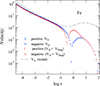 |
Fig. 1. Velocities involved in Eqs. (1) and (2) for iron. The absolute velocity values in cm s−1 are plotted vs. the optical depth. The thick dash-pointed grey curve shows the wind velocity (VW, always positive). VD and VD + Vdrag for the stationary solutions are plotted in blue and red, respectively. Positive velocities have vertical bar markers, and negative velocities have horizontal bar markers. |
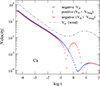 |
Fig. 2. Same as Fig. 1, but for Ca. The velocity curve for the wind is the same as for Fe, and VD is negative in all layers. |
For both iron and calcium, the bump due to ADH is clearly visible around log τ = 0.0. It is particularly remarkable for Ca, since without ADH, the drift velocity (in blue) of Ca is always negative.
5.2.2. Final stationary solutions for the abundances
To compare the stationary solutions obtained with and without ADH, we plot the final stationary abundance stratification in Figs. 3 and 4 (for Fe and Ca, respectively). Without ADH, the two elements are clearly stratified and are over-abundant above log τ = −1.0. A maximum over-abundance is reached at log τ = −2.0, with approximately 0.87 dex for Fe and 0.32 dex for Ca. With ADH, the over-abundances occur at the same depth, but prove somewhat less important: 0.67 dex for Fe, and 0.28 dex for Ca. A most noticeable feature due to ADH consists of the appearance at log τ = 0.0 of under-abundances for both elements; no such abundance drop is found without ADH. These under-abundances may be explained by the upward drag of metal ions, which is caused by ADH creating an abundance hole in these layers. However, the reduced over-abundances above log τ = −1.0 in the presence of ADH are difficult to understand and require a more elaborate analysis.
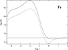 |
Fig. 3. Comparisons of stationary solutions for Fe with and without ADH. The logarithm of the abundance on the [log(NCa/NH) + 12] scale is plotted vs. the logarithm of the optical depth at 5000 Å. The horizontal thick solid grey line is the abundance at t = 0 (homogeneous solar abundance), the solid black curve is the stationary solution for usual atomic diffusion (VD alone), and the dash-pointed curve takes ADH into account (VD + Vdrag). |
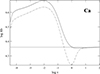 |
Fig. 4. Same as Fig. 3, but for Ca. These curves show the same abundance stratification as the thick solid blue curves of Figs. 5 and 6. |
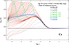 |
Fig. 5. Evolution of the Ca abundance stratification in our Teff = 8500 K, log g = 4.0 atmospheric model, assuming a mass-loss rate of 3.8 10−13 solar mass per year (Z-loss = 8.36 10−15). The horizontal thick solid black line shows the abundance at t = 0 (homogeneous solar abundance), and the thick solid blue curve represents the final stationary solution (t = 7.93 107 years). This is the same stratification as shown by the solid line in Fig. 4. The stratification at intermediate time steps is displayed with thin lines (grey, red, and blue), and a few of them are highlighted (thick green curves); the corresponding ages in years are listed within the drawing area (same colours as the corresponding curves). Three of the four green curves are tagged (1–3) to illustrate the development and subsequent expulsion of a Ca cloud. The dashed thick green line corresponds to the three stratification steps prior to stationarity (towards the end, the evolution slows down markedly). |
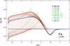 |
Fig. 6. Same as Fig. 5, but with ADH. The thick solid blue curve corresponds to the same stratification as given by the dash-dotted curve in Fig. 4. |
5.2.3. Evolution of the Ca abundance
In order to understand these results (as far as possible for this non-linear process), we need to closely examine the details of the evolution. Because both elements exhibit a similar behaviour, we only considered the case of calcium. We first stress that according to Figs. 1 and 2, the total velocity (Vdrift + VW) is positive at all depths (owing to the wind), which implies an upward flux of calcium throughout the atmosphere.
Fig. 5 displays the evolution of the Ca stratification in the absence of ADH from t = 0 to t = 7.93 107 years (the duration required to reach a stationary solution). This final age represents a theoretical age, based on the assumption that the atmosphere evolves without any disturbance only with the physical processes implemented in our numerical code. The meaning of the various curves is detailed in the legend. It is instructive to comment on the three time-steps that are highlighted with thick green lines and tagged 1–3. Curve 1 reveals that a cloud of Ca forms at a depth of log τ = −2.0 after about 2400 years of diffusion. The over-abundance of Ca in the cloud is relatively large (about twice higher than the final stationary solution). This cloud, evolving through steps 2 and 3, is expelled from the atmosphere in the course of about 2000 years. In the region where this cloud forms, the atmosphere is optically thin and the process of the abundance stratification due to atomic diffusion is no longer local, which drastically increases the non-linear nature of the process. This cloud must be considered as a concentration wave, since its upward motion is about five time faster than the motion of matter dragged by the wind. After this, the stratification evolves gently towards the stationary solution, and no trace of the cloud remains.
Fig. 6 includes ADH, and the evolution of the Ca stratification proceeds in a significantly different way. The cloud (peaks 1–3) of Ca proves much less prominent. We note that the hole at a depth of log τ = 0.0, which is due to ADH, develops immediately from the start of the diffusion process. On account of this hole, fewer Ca atoms are available to fill or maintain the rising cloud (ADH is effective only around log τ = 0.0).
5.3. 3D modelling with magnetic fields
In Sect. 5.2 we examined a plane-parallel model without magnetic fields in order to better understand how ADH affects the time-dependent diffusion of some metals. Since all Ap stars have relatively strong magnetic fields (unlike Am stars, where the fields lie below the detection threshold), often with a predominantly dipolar geometry, we attempt in this section to model the distributions of metals in a magnetic atmosphere with ADH. To do this, we employ the same method as Alecian & Stift (2021) (see their Sect. 2) to construct 3D abundance views for a given magnetic configuration, based on a grid of plane-parallel atmospheric models.
5.3.1. Field geometry
On the one hand, atomic diffusion is extremely sensitive to the field geometry, and the other hand, reliable detailed magnetic geometries of real Ap stars with strong magnetic fields are currently unavailable (see Stift & Leone 2022). We therefore again followed Alecian & Stift (2021) and adopted the geometry of HD 154708 (Stift et al. 2013) (see their comments in their Sect. 3.1). This time, however, we rescaled the magnetic field to a maximum intensity of 5 kG (at the strong magnetic pole), which can be considered typical for Ap stars, with the minimum situated at about 1.27 kG (magnetic lines largely horizontal). This scaling is different from that chosen by Alecian & Stift (2021) because in that paper, we wished to emulate magnetic field intensities close to those of θ Aurigae (as determined by Kochukhov et al. 2019), whose parameters differ significantly from those of the model we consider in the present work. The magnetic field configuration used for our calculations is shown in Figs. 7 and 8. The field geometry corresponds to a non-axisymmetric, tilted, and decentred dipole.
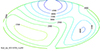 |
Fig. 7. Magnetic field intensity in Gauss (Hammer equal-area projection). |
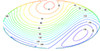 |
Fig. 8. Magnetic field angle with respect to the vertical (horizontal field lines have 90°). |
5.3.2. Ca distribution for stationary solutions
As explained in Alecian & Stift (2021), our method of modelling 3D abundance distributions of metals is based on a grid of plane-parallel, stratified models computed by CARATMOTION. Some metals are assumed to change in abundance due to time-dependent diffusion, and the remaining metals keep their initial homogeneous abundances. The stellar surface is considered as a juxtaposition of facets (around 105 facets in the present work), each of which corresponds to a 1D atmosphere model obtained by interpolation in a grid of the plane-parallel models.
The magnetic configuration being given by a non-axisymmetric, tilted, off-centre dipole, no straightforward relation exists between field intensity and angle. We therefore used a simple empirical approach first described in (Sect. 2.1 Alecian & Stift 2017) and later optimised by Alecian & Stift (2021) for the magnetic geometry of HD 154708. A few established facts are at the basis of our approach: (i) the stratification process varies little for magnetic angles smaller than 60°, they become significantly more sensitive to angles between 80 and 90°. (ii) At the same time, stratification depends in a relatively simple way on the field strength. (iii) The change with atmospheric depth is important: lower densities make for stronger effects of the magnetic field on the diffusion process. Keeping this in mind, we improved upon the grid spacing (field strength and angle) employed in 2017, and thereby reduced the number of models to 706.
In this section, we only discuss 3D models obtained from CARATMOTION runs where stationary solutions were reached for all the specified diffusing metals. All facets are independent of each other since horizontal diffusion is negligible. In our approach there is no exchange of matter between facets. The parameters used to calculate stratification in a given facet differ from those of its neighbours only by the magnetic field angle and intensity. For this exercise, we assumed a homogeneous mass-loss rate over the star of 3.8 10−13 solar mass per year (or Z-loss = 8.36 10−15).
With our adopted parameters, all the models of the grid converged to a stationary solution after around 108 years. The time elapsed to reach a stationary solution may slightly differ from one facet to the next, and models evolve very little close to the stationary solution. The entire atmosphere around the star was divided into slabs according to the depth (in log τ). For the sake of conciseness in the presentation of the results, we divided the atmosphere into four slabs (Fig. 9, with and without ADH) that extended from log τ = −3.0 to log τ = +0.1. The actual optical depth intervals are indicated at the top of each panel. The Ca abundance shown in these panels represents the average abundance in each slab. The calculation for the deepest slab with ADH (last right panel of Fig. 9) shows that there is a patch of under-abundance (in light blue) of Ca around the horizontal magnetic lines (90°) and a field intensity of about 3 kG. This patch does not appear when ADH is neglected (left panels of Fig. 9). This behaviour may be expected from the results shown in Fig. 4, which show a significant under-abundance of Ca around log τ = 0.. The patch of under-abundance in Fig. 9 is less pronounced than in Fig. 4 because the under-abundance is averaged over the depth of the slab. This is a qualitative difference between the two cases. In this deepest slab, the abundance contrast over the star is very low (hardly detectable by spectroscopic observation); but there is about 0.1 dex less Ca in that slab when ADH is taken into account.
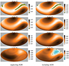 |
Fig. 9. Comparison of all atmosphere of stationary solutions for 3D calcium abundances (tomographic view) without (left panels) and with ADH (right panels) in four contiguous slabs of a magnetic atmosphere, situated between log τ = −3.0 and +0.1 (Hammer equal-area projection). The depth interval of each slab is written at the top of each panel. The dark green colour corresponds to the solar abundance (6.36 ± 10%). The mass-loss rate is assumed to be uniform over the star (3.8 10−13 solar mass per year, or Z-loss = 8.36 10−15). In the last panel on the right, displaying abundances with ADH, Ca is slightly under-abundant (light blue) in some parts of the star at a depth of around log τ = 0.0, as in Fig. 6. In this slab, the Ca abundance differs very little from the solar value. |
5.3.3. Ca distribution for non-stationary solutions
As explained in Sect. 5.2, in order to have stationary solutions for the metals we wished to consider, we constrained the mass-loss rate to lie above a certain value, 3.8 10−13 solar mass per year in the present case. Even though this allowed us to confirm the significant effects of ADH (which is our main purpose), it remained quite frustrating to have to do so because we expect an interesting behaviour for lower mass-loss rates that cannot be excluded for real stars. We therefore decided to carry out calculations with more realistic mass-loss parameters to determine how the abundance stratification evolves over time at least during the first years of time-dependent diffusion up to the age beyond which the code can no longer cope.
Following Babel (1992), Alecian & Stift (2021) considered a mass-loss rate to be a function of the magnetic field angle (see their Fig. 3), that is, a decreasing rate with increasing field angle, the highest wind speed occurring at the magnetic poles. In this section, we adopt the same approach and chose the mass-loss rate profile shown in Fig. 10: A maximum mass-loss rate of 3.0 10−13 (Z-loss = 6.6 10−15) for vertical field lines and a ten times lower rate for horizontal fields. In this simple model, the mass-loss rate only depends on the angle. In the absence of observational evidence, this profile is arbitrary, but it is more realistic than a uniform rate for a magnetic atmosphere.
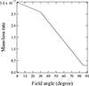 |
Fig. 10. Mass-loss model for the calculations underlying Fig. 11. The mass-loss rate is given in solar mass per year vs. magnetic field angle with respect to the vertical (0° for a magnetic pole). The mass-loss rate is 3.0 10−13 (Z-loss = 6.6 10−15) at the magnetic pole and ten times lower for horizontal magnetic lines (90°). |
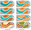 |
Fig. 11. Same as Fig. 9, but assuming the non-uniform mass-loss rates shown in Fig. 10. The abundances of Ca are no longer stationary solutions, but are those reached after 1000 years of diffusion. The similarities between the images can be misleading when the colour scale next to each panel is not taken into account. |
We calculated two more grids of 1D models (with and without ADH, but with the same magnetic parameters as in Sect.5.3.2) using the mass-loss rate model of Fig. 10. As expected, none of the 1D models reached a stationary solution. Depending on the magnetic angle and intensity of a given model in the grid, the calculations stopped at an evolution time of between about 103 and 104 years. This is due to the very strong abundance gradient of iron, which is several orders of magnitude in a narrow depth interval (in log τ) of about 0.5 dex. We finally selected from each grid the stratification attained after approximately 103 years; thus, all the facets making up the stellar surface have an identical evolutionary age. The results are presented in Fig. 11. The abundance contrasts are much stronger than those found for stationary solutions derived for higher mass-loss rates. The differences in the abundance distributions that are derived without and with ADH are also larger.
6. Discussion
6.1. Importance of the ambipolar diffusion of hydrogen
Our numerical results presented in Sect. 5.2 show that ADH significantly affects metal stratification in atmospheres with effective temperatures at which partial ionisation of hydrogen is important. We specifically considered diffusion of three metals (Mg, Si, and Ca) because for these effective temperatures, they are not strongly supported in the atmosphere by the radiation field (weak radiative acceleration, often lower than gravity) which should make them more sensitive to ADH, which gives them an upward push in certain layers. We only discussed the case of Ca because it appears that Mg and Si exhibit very similar behaviour. We included Fe diffusion because the total opacity is more affected by the abundance stratification of iron than by that of any other element; it thus affects the atomic diffusion of all metals. Figs. 3 and 4, quite at variance with our initial hypothesis, showed that ADH is effective not only for Ca (idem for Mg and Si), but also for Fe, even though this element is well supported by the radiation field.
Figs. 5 and 6 reveal a remarkable behaviour during the evolution of the abundances with time. They illustrate how impressively transient phases can differ from the final stationary solution. This constitutes a perfect example of the non-linear build-up of an abundance stratification, which was a well-known fact immediately at the beginning of the studies of time-dependent diffusion. The transient cloud is less prominent when ADH is included, possibly because it helps to prevent a strong abundance gradient from appearing with the current set of input parameters, in particular, with the assumed mass-loss rate.
6.2. Mass-loss rate: A crucial parameter
As discussed in Sect. 2.2, even though an upper limit7 can be assumed for the mass-loss rate that is to be adopted, it still remains a free parameter in our modelling. This represents a major drawback because all our calculations show just how sensitive the process of abundance stratification is to this parameter. For the specific discussion of stationary solutions, we had to adopt the lowest mass-loss rate (3.8 10−13) that allowed us to reach these solutions (for the non-magnetic case), and we note that it is close to the upper limit. We therefore caution that the abundance distributions presented in this work should not be generalised to observed stars without taking their strong dependence on the assumed mass-loss rate into consideration. This is of particular importance for the 3D stationary distribution shown in Fig. 9: It is based on an unrealistically uniform mass-loss rate because the main purpose was to estimate the role of ADH.
In order to obtain a more realistic picture of a 3D distribution over the entire stellar atmosphere, we used non-isotropic (and lower) mass-loss rates, as shown in Fig. 10. This came at a cost, however: We no longer reached stationary solutions. Fig. 11 shows the Ca distribution after 1000 years of diffusion. The Ca over-abundances are observed at the magnetic poles, with a belt of notable under-abundances following horizontal magnetic lines. We do not know how the abundance stratification evolve in this atmosphere beyond a few thousand years of diffusion. As discussed previously, the Fe abundance gradient becomes rather strong. As an example, we show in Fig. 12 the Fe stratification for one of the models in our grid that was used to construct the 3D distributions in Fig. 11 (case with ADH). This model pertains to a magnetic pole (5 kG, 0°), and the iron abundance displayed corresponds to the abundance we derived in the last time step for this specific model (about 4000 years of diffusion8). The abundance of Fe increases strongly from log τ = −2.5 to −2.0: The iron concentration grows by a factor of 100. This causes the simulation algorithm to greatly reduce the time steps, which prevents the calculation from being performed in a reasonable time or even advancing at all.
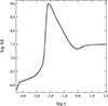 |
Fig. 12. Abundance stratification of Fe at the magnetic pole (5 kG) after about 4000 yr of diffusion. |
6.3. Importance of transient phases
The first generation of studies devoted to the modelling of atomic diffusion in stellar atmospheres (up to the first decade of this century) customarily presented equilibrium solutions (as already mentioned in Sect. 1) because they allow an objective estimate of the effectiveness of this process in producing abundance anomalies in CP star atmospheres. This also makes it possible to confirm whether the diffusion process is compatible with the observed anomalies; but the results cannot be used to predict all of the particular abundances determined for a given CP star. When time-dependent diffusion calculations involving the solution of the continuity equation became technically possible, it made sense to base the improved estimates of the stratification of elements on general stationary solutions (equilibrium solutions constitute the simplest members of this family).
The use of more realistic physics and the temptation to embark on the modelling of observed individual stars are accompanied by a number of difficulties, however, first of which is the increased number of parameters such as the precise knowledge of the magnetic configuration (which also concerns equilibrium solutions), and of the mass-loss model that is to be adopted (which does not apply to equilibrium solutions). A second difficulty is specific to time-dependent diffusion and is linked to the dynamical aspect of abundances stratification. When we are able to find stationary solutions (sometimes facing technical problems that can probably be overcome) and can follow the stratification build-up, we do not know a priori to which stratification stage the atmosphere of an observed Ap star might correspond. This introduces highly undesirable uncertainties, and we recall that very different the transient phases are obtained compared to a final stationary solution. Therefore, the legitimate question arises whether it is still justified to consider general stationary solutions to illustrate the effects of atomic diffusion in CP star atmospheres.
According to the calculations shown in Figs. 3 and 4, the answer may be yes for high enough mass-loss rates because the evolution is fast and the stratification is close to the stationary solutions after a few thousand years of diffusion. However, the answer could rather be no for low mass-loss rates: The stratification presented in Figures 11 and 12 is still very far removed from stationary solutions. Large over-abundances and strong gradients of iron can form in the presence of these mass-loss rates, and we simply do not yet understand how the abundance stratification process will evolve further. It is possible that in some cases, the strong gradients may eventually decrease, allowing a gentle evolution to take over. The time required for this scenario is currently unknown but is expected to be significant, certainly in excess of 104 years, during which the atmosphere must remain stable enough (this also applies to the magnetic configuration), a condition far from guaranteed. Alternatively, large over-abundances and strong gradients of iron (and/or of other metals) may trigger some hydrodynamic instability, for example thermohaline (fingering) convection or turbulence, which leads to a mixing of the medium. In these unstable cases, the instability will disappear when the medium is re-hoomogenised, and the stratification process can restart, which might lead to some type of cyclic behaviour. Furthermore, we cannot exclude a purely diffusive instability because the medium is optically thin (radiation screening)9. In the latter case, the instability would only affect the element that triggered it.
7. Conclusions
Alecian (2023) showed that ambipolar diffusion of hydrogen (ADH) significantly affects the diffusion velocity of metals in the atmospheres of Ap stars when partial ionisation of hydrogen is high. This process essentially concerns cool Ap stars, and it becomes negligible for stars with effective temperatures higher than about 10 000 K. We evaluated the effect of ADH in the process of abundance stratification due to atomic diffusion, which has not been studied before. We considered a typical main-sequence atmosphere with Teff = 8500 K and computed the time-dependent atomic diffusion of four metals (Mg, Si, Ca, and Fe), using our code CARATMOTION. The results with and without ADH were compared.
The abundance stratification process is clearly affected by ADH, not only for metals that are weakly supported by the radiation field such as Mg, Si, and Ca, but also for metals that are strongly supported, such Fe. As a first conclusion, any calculation of atomic diffusion in cool Ap stars must therefore include ADH.
As a second conclusion, we confirm the importance of the mass-loss rate. We confirm that the existence of the CP phenomenon implies that the mass-loss rates in these main-sequence stars must be lower than about 10−12 solar mass per year (non-separated wind, or Z-loss ≲ 2.2 10−14). Due to the lack of observational data, the mass-loss rate is a free parameter in our computations. On the other hand, for numerical reasons, there is a lower limit to this parameter when stationary solutions are sought. This limit is often approximately 3.8 10−13 (Z-loss ≈ 8.36 10−15) for the atmospheric model we considered in this work, depending on the assumed magnetic parameters.
Due to the limitations imposed on CARATMOTION by the mass-loss rate parameter, we were unable to verify the situation that allows ambipolar flooding as discussed by Alecian (2023). This phenomenon cannot be observed when the mass-loss rate is relatively high, which unfortunately is the case for the current version of CARATMOTION.
To illustrate the 3D abundances resulting from mass-loss rates lower than the limit imposed by CARATMOTION, we studied non-stationary stratification, which occurs in a diffusion time shorter than 1000 years for our atmospheric model. The amplitudes of the vertical abundances during the transient phases of the stratification build-up can be far higher than those of the softer final stationary solutions and are arguably as valid as the latter. This induces us to question the value of systematically searching for stationary solutions when modelling time-dependent atomic diffusion in the atmospheres of CP stars, especially when these stationary solutions are only reached after evolution times that approach the lifetime of the star on the main sequence.
This is easily justified, since the layers concerned by our calculations are located too deep for separation to occur.
We denote this point as “virtual” because it does not lie in an atmospheric layer, but rather between the two adjacent layers.
See Morel & Lebreton (2008), Marques et al. (2013), Deal et al. (2018), and the website https://www.ias.u-psud.fr/cesam2k20/home.html
CARATMOTION is entirely written in Ada.
Ap stars are slow rotators, so that gravitational settling of helium can take place in outer layers. This leads to the disappearance (or slowing down) of the outer convection zone, which is a necessary condition for the efficient diffusion of metals in the atmosphere (Michaud 1970; Michaud et al. 2015).
The 70 models of our grid are characterised by the following magnetic parameters: field modulus |B| = 1270, 1650, 2070, 2620, 3310, 4140, 5000 G, angle 0, 30, 60, 70, 75, 80, 83, 85, 87, 90°. Note that the |B| values are scaled intensities from the 2021 paper.
10−12 solar mass per year (non-separated wind).
We recall that the last time step occurs at different times from one model to the next. The abundances in Fig. 11 were obtained at the age of 1000 yr, corresponding to the maximum time in common to the models in the grid.
This instability was proposed by Alecian (1998) (see Sect. 2.2 of this article). An instability like this, plausible as it may appear, has not yet been identified in numerical simulations, however.
Acknowledgments
Most of the codes used to compute our models have been compiled with the GNAT GPL edition of the Ada compiler as provided by AdaCore; this valuable contribution to scientific computing is greatly appreciated. The calculations with the CARATMOTION code have been executed on HPC resources at GENCI-CINES (grants c2023045021). Access has been granted to the HPC resources of MesoPSL, financed by the “Region Ile de France” and the project Equip@Meso (reference ANR-10-EQPX-29-01) of the program “Investissements d’Avenir” supervised by the “Agence Nationale pour la Recherche”. 3D reconstructions have been carried out using the software © IGOR PRO (V9). The authors want to thank Dr. Günther Wuchterl, head of the “Verein Kuffner-Sternwarte”, for the hospitality offered. We are greatly indepted to Morgan Deal who provided the grid of evolutionary tracks used to estimate the stellar masses.
References
- Alecian, G. 1998, CAOSP, 27, 290 [Google Scholar]
- Alecian, G. 2023, MNRAS, 519, 5913 [NASA ADS] [CrossRef] [Google Scholar]
- Alecian, G., & Stift, M. J. 2010, A&A, 516, A53+ [NASA ADS] [CrossRef] [EDP Sciences] [Google Scholar]
- Alecian, G., & Stift, M. J. 2017, MNRAS, 468, 1023 [Google Scholar]
- Alecian, G., & Stift, M. J. 2019, MNRAS, 482, 4519 [Google Scholar]
- Alecian, G., & Stift, M. J. 2021, MNRAS, 504, 1370 [NASA ADS] [CrossRef] [Google Scholar]
- Asplund, M., Grevesse, N., Sauval, A. J., & Scott, P. 2009, ARA&A, 47, 481 [NASA ADS] [CrossRef] [Google Scholar]
- Babel, J. 1992, A&A, 258, 449 [NASA ADS] [Google Scholar]
- Babel, J. 1995, A&A, 301, 823 [Google Scholar]
- Babel, J. 1996, A&A, 309, 867 [Google Scholar]
- Babel, J., & Michaud, G. 1991, A&A, 248, 155 [NASA ADS] [Google Scholar]
- Bischof, K. M. 2005, Mem. Soc. Astron. Ital. Suppl., 8, 64 [Google Scholar]
- Castor, J. I., Abbott, D. C., & Klein, R. I. 1975, ApJ, 195, 157 [Google Scholar]
- Deal, M., Alecian, G., Lebreton, Y., et al. 2018, A&A, 618, A10 [NASA ADS] [CrossRef] [EDP Sciences] [Google Scholar]
- Fišák, J., Kubát, J., Kubátová, B., Kromer, M., & Krtička, J. 2023, A&A, 670, A41 [NASA ADS] [CrossRef] [EDP Sciences] [Google Scholar]
- Kochukhov, O., Shultz, M., & Neiner, C. 2019, A&A, 621, A47 [NASA ADS] [CrossRef] [EDP Sciences] [Google Scholar]
- Krtička, J. 2014, A&A, 564, A70 [NASA ADS] [CrossRef] [EDP Sciences] [Google Scholar]
- Kurucz, R. L. 2005, Mem. Soc. Astron. Ital. Suppl., 8, 14 [Google Scholar]
- LeBlanc, F., Monin, D., Hui-Bon-Hoa, A., & Hauschildt, P. H. 2009, A&A, 495, 937 [NASA ADS] [CrossRef] [EDP Sciences] [Google Scholar]
- Lucy, L. B., & Solomon, P. M. 1970, ApJ, 159, 879 [Google Scholar]
- Marques, J. P., Goupil, M. J., Lebreton, Y., et al. 2013, A&A, 549, A74 [NASA ADS] [CrossRef] [EDP Sciences] [Google Scholar]
- Meyer, J. P. 1985, ApJS, 57, 173 [CrossRef] [Google Scholar]
- Michaud, G. 1970, ApJ, 160, 641 [Google Scholar]
- Michaud, G., Tarasick, D., Charland, Y., & Pelletier, C. 1983, ApJ, 269, 239 [Google Scholar]
- Michaud, G., Richer, J., & Vick, M. 2011, A&A, 534, A18 [NASA ADS] [CrossRef] [EDP Sciences] [Google Scholar]
- Michaud, G., Alecian, G., & Richer, J. 2015, Atomic Diffusion in Stars, Astronomy and Astrophysics Library (Switzerland: Springer International Publishing) [CrossRef] [Google Scholar]
- Morel, P., & Lebreton, Y. 2008, Ap&SS, 316, 61 [Google Scholar]
- Stift, M. J., & Leone, F. 2022, A&A, 659, A33 [NASA ADS] [CrossRef] [EDP Sciences] [Google Scholar]
- Stift, M. J., Hubrig, S., Leone, F., & Mathys, G. 2013, ASP Conf. Ser., 479, 125 [NASA ADS] [Google Scholar]
- Strittmatter, P. A., & Norris, J. 1971, A&A, 15, 239 [NASA ADS] [Google Scholar]
- Vick, M., Michaud, G., Richer, J., & Richard, O. 2010, A&A, 521, A62 [EDP Sciences] [Google Scholar]
All Figures
|
Fig. 1. Velocities involved in Eqs. (1) and (2) for iron. The absolute velocity values in cm s−1 are plotted vs. the optical depth. The thick dash-pointed grey curve shows the wind velocity (VW, always positive). VD and VD + Vdrag for the stationary solutions are plotted in blue and red, respectively. Positive velocities have vertical bar markers, and negative velocities have horizontal bar markers. |
| In the text | |
|
Fig. 2. Same as Fig. 1, but for Ca. The velocity curve for the wind is the same as for Fe, and VD is negative in all layers. |
| In the text | |
|
Fig. 3. Comparisons of stationary solutions for Fe with and without ADH. The logarithm of the abundance on the [log(NCa/NH) + 12] scale is plotted vs. the logarithm of the optical depth at 5000 Å. The horizontal thick solid grey line is the abundance at t = 0 (homogeneous solar abundance), the solid black curve is the stationary solution for usual atomic diffusion (VD alone), and the dash-pointed curve takes ADH into account (VD + Vdrag). |
| In the text | |
|
Fig. 4. Same as Fig. 3, but for Ca. These curves show the same abundance stratification as the thick solid blue curves of Figs. 5 and 6. |
| In the text | |
|
Fig. 5. Evolution of the Ca abundance stratification in our Teff = 8500 K, log g = 4.0 atmospheric model, assuming a mass-loss rate of 3.8 10−13 solar mass per year (Z-loss = 8.36 10−15). The horizontal thick solid black line shows the abundance at t = 0 (homogeneous solar abundance), and the thick solid blue curve represents the final stationary solution (t = 7.93 107 years). This is the same stratification as shown by the solid line in Fig. 4. The stratification at intermediate time steps is displayed with thin lines (grey, red, and blue), and a few of them are highlighted (thick green curves); the corresponding ages in years are listed within the drawing area (same colours as the corresponding curves). Three of the four green curves are tagged (1–3) to illustrate the development and subsequent expulsion of a Ca cloud. The dashed thick green line corresponds to the three stratification steps prior to stationarity (towards the end, the evolution slows down markedly). |
| In the text | |
|
Fig. 6. Same as Fig. 5, but with ADH. The thick solid blue curve corresponds to the same stratification as given by the dash-dotted curve in Fig. 4. |
| In the text | |
|
Fig. 7. Magnetic field intensity in Gauss (Hammer equal-area projection). |
| In the text | |
|
Fig. 8. Magnetic field angle with respect to the vertical (horizontal field lines have 90°). |
| In the text | |
|
Fig. 9. Comparison of all atmosphere of stationary solutions for 3D calcium abundances (tomographic view) without (left panels) and with ADH (right panels) in four contiguous slabs of a magnetic atmosphere, situated between log τ = −3.0 and +0.1 (Hammer equal-area projection). The depth interval of each slab is written at the top of each panel. The dark green colour corresponds to the solar abundance (6.36 ± 10%). The mass-loss rate is assumed to be uniform over the star (3.8 10−13 solar mass per year, or Z-loss = 8.36 10−15). In the last panel on the right, displaying abundances with ADH, Ca is slightly under-abundant (light blue) in some parts of the star at a depth of around log τ = 0.0, as in Fig. 6. In this slab, the Ca abundance differs very little from the solar value. |
| In the text | |
|
Fig. 10. Mass-loss model for the calculations underlying Fig. 11. The mass-loss rate is given in solar mass per year vs. magnetic field angle with respect to the vertical (0° for a magnetic pole). The mass-loss rate is 3.0 10−13 (Z-loss = 6.6 10−15) at the magnetic pole and ten times lower for horizontal magnetic lines (90°). |
| In the text | |
|
Fig. 11. Same as Fig. 9, but assuming the non-uniform mass-loss rates shown in Fig. 10. The abundances of Ca are no longer stationary solutions, but are those reached after 1000 years of diffusion. The similarities between the images can be misleading when the colour scale next to each panel is not taken into account. |
| In the text | |
|
Fig. 12. Abundance stratification of Fe at the magnetic pole (5 kG) after about 4000 yr of diffusion. |
| In the text | |
Current usage metrics show cumulative count of Article Views (full-text article views including HTML views, PDF and ePub downloads, according to the available data) and Abstracts Views on Vision4Press platform.
Data correspond to usage on the plateform after 2015. The current usage metrics is available 48-96 hours after online publication and is updated daily on week days.
Initial download of the metrics may take a while.