| Issue |
A&A
Volume 689, September 2024
|
|
|---|---|---|
| Article Number | A82 | |
| Number of page(s) | 19 | |
| Section | Planets and planetary systems | |
| DOI | https://doi.org/10.1051/0004-6361/202450833 | |
| Published online | 04 September 2024 | |
A study of centaur (54598) Bienor from multiple stellar occultations and rotational light curves*
1
Instituto de Astrofísica de Andalucía – Consejo Superior de Investigaciones Científicas (IAA-CSIC),
Glorieta de la Astronomía S/N,
18008
Granada,
Spain
e-mail: This email address is being protected from spambots. You need JavaScript enabled to view it.
2
Florida Space Institute, UCF,
12354
Research Parkway, Partnership 1 building, Room 211,
Orlado,
USA
3
Federal University of Technology-Paraná (UTFPR/DAFIS),
Av. Sete de Setembro, 3165, CEP
80230-901
Curitiba,
PR,
Brazil
4
Laboratório Interinstitucional de e-Astronomia – LIneA – and INCT do e-Universo. Av. Pastor Martin Luther King Jr,
126 Del Castilho, Nova América Offices, Torre 3000/sala 817 CEP:
20765-000,
Brazil
5
LESIA, UMR8109, Observatoire de Paris, Université PSL, CNRS, Sorbonne Université, Université de Paris,
5 place Jules Janssen,
Meudon
92195,
France
6
Instituto de Física Aplicada a las Ciencias y las Tecnologías, Universidad de Alicante,
San Vicent del Raspeig,
03080
Alicante,
Spain
7
Space Telescope Science Institute,
3700
San Martin Drive,
Baltimore,
USA
8
Institut Polytechnique des Sciences Avancées IPSA,
63 boulevard de Brandebourg,
94200
Ivry-sur-Seine,
France
9
Institut de Mécanique Céleste et de Calcul des Éphémérides, IMCCE, Observatoire de Paris, PSL Research University. CNRS, Sorbonne Universités, UPMC Univ.
Paris 06, Univ. Lille, 77 Av. Denfert-Rochereau,
75014
Paris,
France
10
naXys, Department of Mathematics, University of Namur,
Rue de Bruxelles 61,
Namur
5000,
Belgium
11
Universidade Federal do Rio de Janeiro, Observatório do Valongo,
Ladeira Pedro do Antonio 43,
Rio de Janeiro,
RJ
20.080-90,
Brazil
12
UNESP – São Paulo State University,
Grupo de Dinâmica Orbital e Planetologia,
Guaratinguetá,
SP
12516-410,
Brazil
13
Observatório Nacional (MCTI), Rua Gal. José Cristino,
77–Bairro Imperial de São Cristóvão,
20921-400
Rio de Janeiro,
Brazil
14
TÜBİTAK National Observatory, Akdeniz University Campus,
07058
Antalya,
Turkey
15
Astronomy Department and Van Vleck Observatory, Wesleyan University,
Middletown,
CT
06459,
USA
16
Westport Astronomical Society,
Westport,
CT,
USA
17
Dept of Mathematics and Physics, University of New Haven,
West Haven,
CT,
USA
18
Salvia Observatory,
France
19
Schreurs O (S.A.L.),
Liège,
Belgium
20
Société Astronomique de Liège (S.A.L.),
Nandrin Observatory,
Belgium
21
Dourbes,
Viroinval,
Belgium
22
Tsu Mie,
Tsu Mie,
Japan
23
Pressigny,
France
24
Uda Nara,
Nara,
Japan
25
Owase Mie,
Nakamuracho,
Japan
26
Cottered Observatory,
Hertfordshire,
England, UK
Received:
22
May
2024
Accepted:
12
July
2024
Abstract
Context. Centaurs, distinguished by their volatile-rich compositions, play a pivotal role in understanding the formation and evolution of the early Solar System, as they represent remnants of the primordial material that populated the outer regions. Stellar occultations offer a means to investigate their physical properties, including shape and rotational state, and the potential presence of satellites and rings.
Aims. This work aims to conduct a detailed study of the centaur (54598) Bienor through stellar occultations and rotational light curves from photometric data collected during recent years.
Methods. We successfully predicted three stellar occultations by Bienor that were observed from Japan, Western Europe, and the USA. In addition, we organized observational campaigns from Spain to obtain rotational light curves. At the same time, we developed software to generate synthetic light curves from three-dimensional shape models, enabling us to validate the outcomes through computer simulations.
Results. We resolved Bienor’s projected ellipse for December 26, 2022; determined a prograde sense of rotation; and confirmed an asymmetric rotational light curve. We also retrieved the axes of its triaxial ellipsoid shape as a = (127 ± 5) km, b = (55 ± 4) km, and c = (45 ± 4) km. Moreover, we refined the rotation period to 9.1736 ± 0.0002 h and determined a geometric albedo of (6.5 ± 0.5)%, which is higher than previously determined by other methods. Finally, by comparing our findings with previous results and simulated rotational light curves, we analyzed whether an irregular or contact-binary shape, an additional element such as a satellite, or significant albedo variations on Bienor’s surface may be present.
Key words: occultations / Kuiper belt objects: individual: Centaurs / Kuiper belt objects: individual: (54598) Bienor / Kuiper belt objects: individual: trans-Neptunian Object
Movies associated to Figs. 6 and D.1 are only available https://www.aanda.org
© The Authors 2024
 Open Access article, published by EDP Sciences, under the terms of the Creative Commons Attribution License (https://creativecommons.org/licenses/by/4.0), which permits unrestricted use, distribution, and reproduction in any medium, provided the original work is properly cited.
This article is published in open access under the Subscribe to Open model. This email address is being protected from spambots. You need JavaScript enabled to view it. to support open access publication.
1 Introduction
Among the small bodies of the Solar System exist the so-called centaurs, some of which are characterized by their combination of cometary and asteroidal features. It has been theorized that centaurs were originally trans-Neptunian objects (TNOs) expelled due to gravitational scattering by Neptune (Holman & Wisdom 1993; Duncan et al. 1995; Duncan & Levison 1997). These objects, transient in nature, have an average lifespan of only a few million years (Horner et al. 2004), primarily because of their gravitational interactions with the giant planets that lead to their eventual expulsion from the region. Therefore, centaurs present a unique opportunity to study TNOs and provide a better characterization of their physical properties.
The first centaur discovered was Chiron in 1977, although its cometary properties were not identified until a decade later – to date, comet activity has been confirmed in ~ 13% of cases (Bauer et al. 2008). Since the discovery of a second object in 1992, (5145) Pholus, hundreds1 of centaurs have been discovered, although the number depends on the criteria used for their definition. There is not a universally accepted definition of centaurs. Several criteria can be found in the literature, such as having a semi-major axis between 5 and 30 au or those presenting a Tisserand parameter larger than three and a semi-major axis larger than the semi-major axis of Jupiter. Some estimations suggest that there are more than 40 000 centaurs larger than 1 km in diameter, although other authors have estimated that there are more than 100 million (Di Sisto & Brunini 2007).
In a study by Lacerda et al. (2014), more than 100 TNOs and centaurs were examined for their color-albedo distribution. The study identified two clusters: one characterized by dark-neutral objects with a geometric albedo (pV) of approximately ~5% and another composed of bright red objects with geometric albedos exceeding 6%. This division based on color-albedo distribution has been particularly pronounced among centaurs (Bauer et al. 2013; Duffard et al. 2014b; Tegler et al. 2016), with median albedos of approximately ~5% for the dark-neutral group and ~8.4% for the bright red group (Müller et al. 2020).
Due to the large geocentric distances of these small bodies and the consequent challenges in their study, we have only a limited understanding of the physical properties of these objects thus far. To date, through the technique of stellar occultations, we have gathered data on the shape and spatial orientation of the centaur Chariklo (Leiva et al. 2017; Morgado et al. 2021). Moreover, a three-dimensional morphology has been postulated for the centaur Chiron under the assumption of hydrostatic equilibrium (Braga-Ribas et al. 2023). There are also constraints regarding the shapes of centaurs 2002GZ32 (Santos-Sanz et al. 2021; Strauss et al. 2021) and Echeclus (Rousselot et al. 2021; Pereira et al. 2024). In addition to their morphology, stellar occultations have revealed that at least two centaurs, Chariklo and Chiron, possess rings (Braga-Ribas et al. 2014; Ortiz et al. 2015, 2023).
The centaur (54598) Bienor (q = 13.19 au, Q = 19.90 au, i = 20.74°) is an inactive centaur that was discovered by the Deep Ecliptic Survey in 2000 (Elliot et al. 2005). It has an orbital period of 67.34 yr and a rotation period of ~9.14 h (Ortiz et al. 2002). Near-infrared spectral measurements have indicated the presence of water ice on its surface (Dotto et al. 2003; Guilbert et al. 2009). A geometric albedo of (5.0 ± 1.9)% (Bauer et al. 2013) together with the fact that its B-V color is 1.12 ± 0.03 (Tegler et al. 2008) place Bienor within the dark-neutral group. Extreme light curve amplitudes (DeMeo et al. 2009) suggest Bienor to be a highly elongated body. According to Fernández-Valenzuela et al. (2017), the orientation of its rotational pole is βp = 50° ± 3°, λp = 35° ± 8° (prograde rotation) or βp = −50° ± 3°, λp = 215° ± 8° (retrograde rotation). Assuming Bienor is a triaxial ellipsoid under hydrostatic equilibrium, they constrained the b/a axial ratio to 0.45 ± 0.05 and a density of 594 kg m−3, although other solutions are also feasible.
Some controversy surrounds this object due to discrepancies in size and albedo obtained through different techniques (Lellouch et al. 2017). Through thermal measurements, Bauer et al. (2013), using data from the Wide-field Infrared Survey Explorer (WISE), obtained (187.5 ± 15.5) km of diameter and a geometric albedo of (5.0 ± 1.9)%; Duffard et al. (2014a) retrieved ![Mathematical equation: $\[198_{-7}^{+6}\]$](/articles/aa/full_html/2024/09/aa50833-24/aa50833-24-eq1.png) km of diameter and a geometric albedo of
km of diameter and a geometric albedo of ![Mathematical equation: $\[4.3_{-1.2}^{+1.6}\]$](/articles/aa/full_html/2024/09/aa50833-24/aa50833-24-eq2.png) using radiometric measurements from the Herschel Space Observatory and Spitzer Space Telescope; and Lellouch et al. (2017) obtained from Spitzer, Herschel, and ALMA observations a diameter of 179–184 ± 6 km and a geometric albedo of
using radiometric measurements from the Herschel Space Observatory and Spitzer Space Telescope; and Lellouch et al. (2017) obtained from Spitzer, Herschel, and ALMA observations a diameter of 179–184 ± 6 km and a geometric albedo of ![Mathematical equation: $\[5.3_{-1.6}^{+1.8}\]$](/articles/aa/full_html/2024/09/aa50833-24/aa50833-24-eq3.png) . However, Fernández-Valenzuela et al. (2023) estimated an area-equivalent diameter of 150 ± 20 km using the stellar occultation technique. This is smaller than the thermal diameters and suggestive of a possible satellite or binarity. Moreover, the authors reported a strong irregularity in one of the minima of the rotational light curve, regardless of the aspect angle, but there is nothing compatible with the presence of rings or satellites within their data. Nevertheless, they did not discard a satellite or a ring system similar to that of the centaurs Chariklo and Chiron due to the low signal-to-noise ratio of the observations.
. However, Fernández-Valenzuela et al. (2023) estimated an area-equivalent diameter of 150 ± 20 km using the stellar occultation technique. This is smaller than the thermal diameters and suggestive of a possible satellite or binarity. Moreover, the authors reported a strong irregularity in one of the minima of the rotational light curve, regardless of the aspect angle, but there is nothing compatible with the presence of rings or satellites within their data. Nevertheless, they did not discard a satellite or a ring system similar to that of the centaurs Chariklo and Chiron due to the low signal-to-noise ratio of the observations.
These discrepancies and irregularities have sparked a question about the possible presence of a ring or satellite or the possibility that Bienor is a binary system. The objective of this study is to delve further into this issue. For that, as part of our global collaboration to detect stellar occultations by outer Solar System bodies, we successfully predicted and observed three positive occultations that took place on February 6 and December 26, 2022, and on February 14, 2023. Alongside these data, we have also conducted several observational campaigns to obtain two new rotational light curves that complement the occultation data. In this work, we present our observations and their corresponding technical details in Section 2, followed by the data analysis outcomes in Section 3. Section 4 introduces our software for simulating synthetic rotational light curves, and then it is applied to contextualize the preceding results. Finally, in Section 5, we discuss our findings and check various hypotheses that would explain the discrepancies with the results obtained by other authors through different methods, and we summarize the conclusions we have drawn in Section 6.
Occulted stars by Bienor presented in this work.
2 Observations
2.1 Stellar occultations
The primary predictions of stellar occultations by Bienor were performed using the Numerical Integration of the Motion of an Asteroid (NIMA) solution (Desmars et al. 2015). Subsequently, after a series of observational campaigns carried out during the last years (see Fernández-Valenzuela et al. 2023), Bienor’s orbit was updated and refined. This has allowed for the prediction and observation of three positive occultations in 2022 and 2023 described in the following sections.
2.1.1 Occultation A – February 6, 2022
On February 6, 2022, an occultation by Bienor of the star Gaia DR3 202357903847210880 (see Table 1) was predicted to happen at 08:52:54 UT (referred to hereafter as “Occ. A”), with a maximum duration of 14.7 s in the centrality. The event was observed from two different locations, resulting in positive detections from Middletown and Westport (Connecticut, USA), as shown in Fig. 1a. Table B.1 expands on the information regarding location, instrumentation, and observers involved. Time series observations were obtained and time synchronized using Network Time Protocol (NTP) servers or global positioning systems (GPS) devices. Image acquisition started at least ~5 min before and ended ~5 min after the predicted time. No filters were used to maximize the S/N of the occulted star.
The diameter of the occulted star was estimated using the following equation (van Belle 1999):
![Mathematical equation: $\[\theta=\frac{10^{a+b(V-K)}}{10^{V / 5}},\]$](/articles/aa/full_html/2024/09/aa50833-24/aa50833-24-eq4.png) (1)
(1)
with (a, b) = (0.5, 0.264) for main-sequence stars, (0.669, 0.223) for giant and supergiant stars, and where V and K denote the apparent magnitudes of the star in the V-band and K-band, respectively. According to Zacharias et al. (2004), V = 12.93 mag and K = 10.36 mag. Consequently, because the occulted star is a giant (see Fig. A.1), the angular diameter is computed as 0.0453 mas, corresponding to 0.44 km at a Bienor’s geocentric distance (Δ) of 13.39 au. Because λ is ~600 nm for our CCD/CMOS observations, from Eq. (2), the Fresnel scale of this object is calculated as 0.78 kilometers,
![Mathematical equation: $\[F=\sqrt{\frac{\lambda \Delta}{2}}.\]$](/articles/aa/full_html/2024/09/aa50833-24/aa50833-24-eq5.png) (2)
(2)
The minimum cycle time (exposure plus dead time) here comes from the observation made in Westport, which was recorded as 0.25 s. With Bienor’s velocity at the time of occultation measured at 12.81 km/h, this cycle time corresponds to a distance of 3.20 km. Given that this distance is an order of magnitude greater than that derived from the star’s angular size and Fresnel diffraction effects, they have a small impact on the derivation of ingress and egress times.
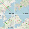 |
Fig. 1 Predicted occultation shadow path computed for February 6, 2022 (a), December 26, 2022 (b & c), and February 14, 2023 (d). Green lines depict the boundaries of the shadow paths, while the gray lines represent the uncertainty in the path resulting from orbital uncertainties. A red line denotes the center of the shadow path, and the pins indicate the positions of the stations involved in the campaigns. Green pins signify sites where a positive occultation was observed. The maps were generated using OpenStreetMap via the Occultation Portal. The dotted arrow denotes the shadow’s direction of motion. |
2.1.2 Occultation B – December 26, 2022
On December 26, 2022, an occultation by Bienor of the star Gaia DR3 961233167113907328 (Table 1) with a maximum duration of 8.6 s was predicted to happen at 20:13:44 UT (hereafter “Occ. B”). The star was observed from seven locations, all reporting positive detections (Figs. 1 b and c). The telescopes were in Western Europe and Japan (see Appendix A and Table B.1). Time series observations were obtained and synchronized using GPS devices. Image acquisition started at least ~5 min before and ended ~5 min after the predicted time. No filters were used to maximize the S/N of the star.
A diameter of 0.0132 mas of the occulted star was estimated using Eq. (1) (giant star, see Fig. A.1), with V = 13.98 mag and K = 12.87 mag from Zacharias et al. (2004). It corresponds to 0.12 km at Bienor’s geocentric distance, Δ, of 12.81 au. The Fresnel scale in this case is 0.76 km. Because the minimum cycle time for these observations is 0.16 s, while Bienor’s velocity at the time of occultation was 21.76 km/h, it translates to a distance of 3.48 km. Thus, the main source of uncertainty comes from the ingress and egress times of the photometric data.
2.1.3 Occultation C – February 14, 2023
On February 14, 2023, an occultation by Bienor of the star Gaia DR3 193308850132660224 (Table 1) with a maximum duration of 14.6 s was predicted at 01:43:46 UT (referred to hereafter as “Occ. C”). The star was observed from two telescopes, resulting in both cases in positive detections. The telescopes were located in Belgium and England (see Fig. 1d and Table B.1). Time series observations were obtained and synchronized using GPS devices. Image acquisition started at least ~5 min before and ended ~5 min later than the predicted time. No filters were used to maximize the S/N of the star.
A diameter of 0.0033 mas of the occulted star was estimated using Eq. (1) (main-sequence star, see Fig. A.1), with V = 16.45 mag and K = 15.26 mag from Zacharias et al. (2004). This corresponds to 0.03 km at Bienor’s geocentric distance, Δ, of 13.16 au. The Fresnel scale in this case is 0.77 km. Because the minimum cycle time for these observations is 1.603 s, while Bienor’s velocity at the time of occultation was 12.87 km/h, it translates to a distance of 20.6 km. Given that this distance is orders of magnitude greater than that derived from the star’s angular size and Fresnel diffraction effects, they have a small impact on the derivation of ingress and egress times.
2.2 Rotational light curves
To determine the rotational phase of Bienor at the moment of the occultations, photometric data were collected in 2021 and 2023 using the 1.5 m telescope at the Sierra Nevada Observatory (OSN) and the 1.23 m telescope at the Calar Alto Observatory (CAHA). The OSN 1.5 m telescope has a 2k×2k CCD with a field of view (FoV) of 7.92′ × 7.92′ and a pixel scale of 0.232″/pixel. The CAHA 1.23 m telescope has a 4k×4k CCD with an FoV of 21.5′ × 21.5′ and a pixel scale of 0.315″/pixel. In both cases, 2×2 binning was used.
Observations of Bienor were conducted at OSN on October 8, 9, 10, 16, 18, 19, and 20 of 2021 and followed by another set of observations on December 12 and 13 of 2023. At CAHA, observations were carried out on October 11, 12, and 21 of 2021 and November 14 and 15 of 2023. An exposure time of 300 s and an R Johnson filter was used in all the observations made with these telescopes.
3 Data analysis and results
3.1 Stellar occultations
The data were compiled and managed through the Tubitak Occultation Portal website (Kilic et al. 2022). First, images were bias and flat-field calibrated using standard procedures with the AstroImageJ software (AIJ) (Collins et al. 2017). For those cases in which the observations were recorded in video format, we used the Planetary Imaging Preprocessor (PIPP2) software to convert them to FITS before performing the photometry.
Next, we performed time series multi-aperture differential photometry with AIJ, measuring the flux of the occulted star (blended with Bienor) and dividing by the comparison stars selected in the FoV. This allowed for the minimization of the systematic photometric errors due to atmospheric variability. As the event only lasted several seconds, flux variations due to the rotational variability of the body did not affect the resulting light curve. We chose an aperture and sky background inner and outer radius to minimize the noise of the data outside the main flux drop due to the occultation. We derived the error bars from Poisson noise calculations, and the results were scaled to the standard deviation of the data (see for details Ortiz et al. 2020). Finally, ingress and egress timing and their uncertainties were computed using the Python occultation timing extractor (PyOTE3, v5.5.1) software package.
The light curves obtained are shown in Figs. B.1, B.2, B.3, B.4. Table B.2 shows the extracted ingress and egress times along with their respective uncertainties.
To project the occultation chords in the sky plane, we needed to translate the ingress and egress time values by using the astro-metric right ascension and declination of Bienor with respect to the observing sites (ICRF frame, JPL#71 ephemerids). For that, we used the JPL Horizons online solar system data and ephemeris computation service4. We then subtracted the value of these coordinates (extremities values of the chords) from the value of the occulted stars’ coordinates, and we converted this difference into kilometers in the sky plane defined by Bienor at its geocentric distance. The result for each occultation is shown in Figs. 2a, 2b, and 2c. All plots present the same vertical and horizontal scale (320 × 320 km) for better comparison.
Because the general equation of an ellipse (conic section) has five degrees of freedom – two for the position of the center (x0, y0), two for the lengths of the semi-major and semi-minor axes (u, v), and one for the rotation of the ellipse or position angle – we needed at least five points to find a unique solution; otherwise, the solution degenerates. Thus, we could only fit an ellipse to the extreme of the chords obtained on December 26, 2022. For that, we used the numerically stable and non-iterative least-squares algorithm defined by Halíř & Flusser (1998). The resulting ellipse along with the chords is shown in Fig. 2b. To propagate the ingress and egress time uncertainties into this fitted ellipse, we ran a Monte Carlo algorithm by generating 1000 random clone extreme points following a Gaussian distribution centered at the value of the chord endpoint and with a width equal to the error in each case. For each cloned solution, we fit an ellipse so that the final parameters of the ellipse (Table 2) are determined by the average value obtained from the 1000 solutions, with the error represented by the standard deviation. The choice of 1000 clones was because we empirically confirmed that at this value, the parameters have reached convergence and that further increasing the number of clones does not enhance the precision of the outcome. The result is that Bienor is a highly elongated triaxial ellipsoid, which is compatible with the range of solutions given in Fernández-Valenzuela et al. (2017).
Finally, using the rotation pole solutions given by Fernández-Valenzuela et al. (2017) and Bienor ephemerides at each occultation time, we computed both the aspect angle and the position angle of the rotation pole (prograde and retrograde). The result is shown in Table 3.
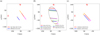 |
Fig. 2 Chords of the stellar occultations projected on the sky plane. The ingress uncertainties are shown in pink, and the egress uncertainties are in orange. The values in parenthesis are the lengths of the chords. (a) Occ. A on February 6, 2022. The minimum distance between the chords is 71.49 km. (b) Occ. B on December 26, 2022. The dashed line describes the ellipse that best fits the points. (c) Occ. C on February 14, 2023. The minimum distance between the chords is 15.35 km. The dashed arrow in the upper-right corner indicates the direction of the shadow motion. |
Parameters of the fitted ellipse for the chords obtained on December 26, 2022.
3.2 Rotational light curves
We corrected the images from bias and flat-field using the same tools and standard procedures described in Section 3.1. Subsequently, we performed time series multi-aperture differential photometry by selecting the same reference stars set within each observation run.
To compute the rotational phase, ϕ, we applied Eq. (3):
![Mathematical equation: $\[\phi=\frac{J D-J D_0}{P},\]$](/articles/aa/full_html/2024/09/aa50833-24/aa50833-24-eq6.png) (3)
(3)
where JD is the Julian date of each image, JD0 is an arbitrary initial date, and P is the sidereal rotational period. All times in this equation were corrected for light travel time. We note that in this work the rotational phase is computed such that it corresponds to zero when the light curve reaches maximum brightness.
Fernández-Valenzuela et al. (2017) determined a synodic period for Bienor of 9.1713 ± 0.0002 h. However, this value does not fit our data. For example, using 2021 photometric data, we determined a rotational phase value of Bienor during the Occ. B of 0.42 ± 0.02; while using 2023 data, the phase value was 0.96 ± 0.02.
We first suspected that it could be due to the difference between synodic and sidereal periods. As discussed by Harris et al. (1984), the phase angle bisector (PAB), that is, the line that bisects the heliocentric and geocentric direction to the small body, serves as an approximation to estimate the difference between the sidereal and synodic periods. It can be determined by applying Eq. (4):
![Mathematical equation: $\[\begin{aligned}&\left|P_{{syn }}-P_{{sid }}\right| \sim \frac{\Delta p}{2 \pi} \frac{P_{s y n}{ }^2}{\Delta t}\end{aligned}\]$](/articles/aa/full_html/2024/09/aa50833-24/aa50833-24-eq7.png) (4)
(4)
where Δp represents the longitude variation of the PAB and Δt is the time span of observations to derive Psyn. This equation is invalid when the small body has a nearly polar aspect, but here it is not the case (see Table 3).
We computed the PBA longitude variation during the period of time in which the observations to derive the synodic period were made (i.e., from June 12, 2013, to August 8, 2016). During this time range, Δp was 18.93°, and according to Eq. (4), |Psyn − Psid|~ 0.00018 h, the same order of magnitude as the error associated with the synodic rotational period, insufficient value to explain the discrepancy.
Then, we employed the Lomb algorithm (Lomb 1976), a variant of the Fourier spectral analysis as coded by Press et al. (1992), to identify the rotation period with our new photometric data. The resulting periodogram is depicted in Fig. 3, wherein the best-fitting solution corresponds to a rotation period of (9.1736 ± 0.0002) h (red line). We observed that another very close solution appears with virtually the same spectral power, which coincides with the solution given by Fernández-Valenzuela et al. (2017) (blue line), thus explaining the discrepancy.
Finally, we folded the data so that the rotational light curves start at the absolute maximum. Then we fit the data points to a second-order Fourier function as follows:
![Mathematical equation: $\[m(\phi)=\sum_{n=0}^i a_{\mathrm{n}} \cos (n \pi \phi)+b_{\mathrm{n}} \sin (n \pi \phi),\]$](/articles/aa/full_html/2024/09/aa50833-24/aa50833-24-eq8.png) (5)
(5)
with i = 2.
The Fourier coefficients are presented in Table 4. Figures 4a and 4b display the rotational light curves for 2021 and 2023, respectively. The vertical lines within each plot denote the rotational phase for individual occultations. Dashed gray lines represent the uncertainty resulting from the propagation of a 0.0002-h error over time. At the bottom of each plot, the residual difference between the modeled curve and observational data are depicted. To calculate the rotational phase of Occ. A, we utilized the 2021 rotational light curve, while for Occ. B and C, we relied on the 2023 light curve. This choice is based on the proximity of these datasets in time, resulting in lower error propagation. Specifically, Occ. A occurred 108 days after collecting the 2021 data. In contrast, Occ. B and C are separated by 323 and 275 days, respectively, from the date of the 2023 data collection. Table 5 shows the rotational phase values along with the propagated period error.
As noted by Fernández-Valenzuela et al. (2023), the asymmetry in the minima of the rotational light curves is still present, given that in both curves the absolute minimum presents a ~45% deeper drop than the other one. Moreover, the light-curve amplitude (Δm) increased from 0.23 ± 0.01 in 2021 to 0.30 ± 0.01 in 2023.
Bienor aspect angle (ψ) and position angle of the rotation pole (θp) for prograde (1) and retrograde (2) solutions.
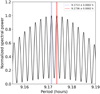 |
Fig. 3 Lomb periodogram’s spectral power obtained from photometric data collected in 2021 and 2023. There are two possible solutions that are very close in spectral power. The solution that best fits with the 2021 and 2023 rotational light curves is the one marked in red, (9.1736 ± 0.0002) h. |
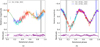 |
Fig. 4 Rotational light curves of Bienor. In (a), we present the rotational light curve using 2021 data, while (b) shows the 2023 observational data. The vertical line indicates the rotational phase during Occ. A, B, and C, respectively. In both panels, the dashed lines show the uncertainty after studying how the 0.0002 h error propagates with time. A unique color represents each observation day. At the bottom, the difference (residual) between the modeled curve and the observational data is shown. |
Rotational phase values of the occultations analyzed in this work.
3.3 Geometric albedo
Using the projected shape of Bienor during Occ. B, we retrieved the area-equivalent diameter (D), which is (149 ± 4) km. On the date of Occ. B, the value of Bienor’s average visual magnitude (HV) was 7.60 ± 0.04 (Fernández-Valenzuela et al. 2017). From the rotational light curve (Fig. 4b) at the time of the occultation, Bienor’s magnitude was 0.12 units higher than the average, corresponding to an instantaneous HV of 7.72 ± 0.04. Using these values in Eq. (6) (Russell 1916),
![Mathematical equation: $\[\sqrt{p_V}=\frac{C}{D} 10^{-H_V / 5},\]$](/articles/aa/full_html/2024/09/aa50833-24/aa50833-24-eq9.png) (6)
(6)
where C = 1330 ± 18 km is a constant (Masiero et al. 2021), we determined pV = 6.5 ± 0.5%, which is larger than the ![Mathematical equation: $\[5.0 ~\pm~1.9 \%, ~4.3_{-1.2}^{+1.6} \% ~\text { or }~ 5.0{-}5.3_{-1.6}^{+1.8} \%\]$](/articles/aa/full_html/2024/09/aa50833-24/aa50833-24-eq10.png) of previous thermal estimates from Bauer et al. (2013); Duffard et al. (2014a); Lellouch et al. (2017), respectively.
of previous thermal estimates from Bauer et al. (2013); Duffard et al. (2014a); Lellouch et al. (2017), respectively.
3.4 3D shape and sense of rotation
From Magnusson (1986), the mathematical relationship between the major and minor axes of the projected ellipse (u, v), aspect angle (ψ), rotational phase (ϕ), and the absolute value of the axes of the ellipsoid a, b and c is given by:
![Mathematical equation: $\[u=\left(\frac{2 A}{-B-\sqrt{B^2-4 A}}\right)^{1 / 2} \quad v=\left(\frac{2 A}{-B+\sqrt{B^2-4 A}}\right)^{1 / 2},\]$](/articles/aa/full_html/2024/09/aa50833-24/aa50833-24-eq11.png) (7)
(7)
where:
![Mathematical equation: $\[\begin{aligned}A= & b^2 c^2 \sin ^2 \psi \sin ^2 \phi+a^2 c^2 \sin ^2 \psi \cos ^2 \phi+a^2 b^2 \cos ^2 \psi \\-B= & a^2\left(\cos ^2 \psi \sin ^2 \phi+\cos ^2 \phi\right)+b^2\left(\cos ^2 \psi \cos ^2 \phi+\sin ^2 \phi\right) \\& +c^2 \sin ^2 \psi.\end{aligned}\]$](/articles/aa/full_html/2024/09/aa50833-24/aa50833-24-eq12.png)
From u, v, ψ, and ϕ derived from Occ. B, we conducted a χ2 minimization based on a grid search for the absolute axes a, b, and c through Eq. (7). We constrained the search so that Δm is within the light curve range determined in 2021 and 2023, that is, 0.23 and 0.30 mag, and then we explored all feasible solutions of u and v, ensuring that χ2, which considers both the values and errors of u and v, as well as the elongation (b/a) and flattening (c/b) metrics as described by Fernández-Valenzuela et al. (2017) were minimized. We find that the solution that best fits all the parameters is given by a=(127 ± 5) km, b=(55 ± 4) km, and c=(45 ± 4) km.
Assuming this solution, we calculated the projected area of Bienor during the date of the observations that led Lellouch et al. (2017) to determining an effective area of 179–184 ± 6 km. These observations were conducted using both Herschel and ALMA in 2011 and 2016. The aspect angles of Bienor on these dates were 140.42° and 147.05°, respectively, with 143.73° being the intermediate aspect angle. Then, we determined the average value of the projected ellipse axes for a complete rotation, resulting in u = (116.73 ± 4.41) km and v = (53.18 ± 3.59) km. This gave us a Bienor area-equivalent diameter of (158 ± 16) km, which is lower than the aforementioned estimation.
Finally, the position angle of the minor axis of the projected ellipse relative to the rotation pole (γ) could be computed using the following equation (Magnusson 1986):
![Mathematical equation: $\[\gamma=\frac{1}{2} \tan ^{-1}\left(\frac{2 ~\cos ~\psi ~\cos ~\phi ~\sin \phi\left(\frac{b^2}{a^2}-1\right)}{\cos ^2 \psi ~\sin ^2 \phi-\cos ^2 \phi+\frac{b^2}{a^2}\left(\cos ^2 ~\psi ~\cos ^2 \phi-\sin ^2 \phi\right)+\frac{c^2}{a^2} ~\sin ^2 \psi}\right).\]$](/articles/aa/full_html/2024/09/aa50833-24/aa50833-24-eq13.png) (8)
(8)
And from γ, we determined the position angle of the minor axis of the projected ellipse with respect to the equatorial north, θv, which is given by:
![Mathematical equation: $\[\theta_v=\theta_p+\gamma.\]$](/articles/aa/full_html/2024/09/aa50833-24/aa50833-24-eq14.png) (9)
(9)
We obtained θν = 280.5° and θv = 176.68° respectively for the prograde and retrograde solutions. In Fig. 5, we plot both solutions (gray arrows) and compare them to the minor axis of the fitted ellipse (denoted by a dashed line). As can be seen, only the prograde rotation is compatible with the Occ. B fitted ellipse. Therefore, we determined that the sense of rotation of Bienor is prograde, excluding the retrograde solution. We note that this is the first time that the rotational sense of a centaur has been determined.
4 Synthetic rotational light curves
The application of light curve inversion for determining the shape of small bodies has primarily been confined to main belt asteroids (Ostro et al. 1988; Durech et al. 2010). However, this method faces limitations when applied to centaurs or TNOs, owing to the need of observing these bodies from multiple angles and maintaining consistent sampling. These requirements pose significant challenges due to the considerable distance, small size, and slow movement across the sky of such objects and render the approach unfeasible (e.g. Showalter et al. 2021).
We employed an alternative technique known as forward modeling. In this approach, we constructed a shape model based on the known axis ratios of Bienor and the shape inferred from the previous occultations outlined in this study. Then, we simulated its rotation as it would be observed from Earth for each occultation date. While we acknowledge that a light curve does not yield a unique interpretation, the available dataset is sufficient to address the issue from this perspective. The main goal of this technique is not about obtaining numerical results but rather combining all the results obtained through different approaches to check whether they are compatible or not.
Initially, we constructed a triaxial ellipsoid shape model with semi-axis a > b > c, where a = 1 and b and c are given from the ratios provided by Fernández-Valenzuela et al. (2017), that is, b/a = 0.45 and c/b = 0.79. This was done through the Blender5 software, which offers the capability to execute Python scripts. The resulting ellipsoidal shape model comprises a triangular mesh with 920 facets, which provides adequate spatial resolution without excessively extending the calculation time.
Next, through JPL Horizons, we obtained the ecliptic Cartesian coordinates of Bienor, the Earth, and the Sun for each respective date. We wrote a Python-based software using the Poly3DCollection package of Matplotlib (Hunter 2007) to orient the shape model such that its rotation pole aligns with the specified values of βp = 50° and λp = 35° (Fernández-Valenzuela et al. 2017). This allowed us to generate an image of the body as seen from Earth and illuminated by the Sun according to the relative positional values.
From the positions of the three bodies, we generated photometric backplanes to calculate the incidence, emission, and phase values for each facet. Then, we determined the radiance that represents the radiant flux reflected per unit solid angle and unit projected area. This calculation assumes a Lambertian surface, meaning that the radiance remains constant regardless of the angle from which it is viewed, resulting in isotropic radiation. Finally, the software generated 2D images of the ellipsoid in the sky plane, with north toward the top of the FoV and east toward the left, as it would be seen from Earth. These images allowed us to visualize the evolution of the small body at different temporal scales, enabling us to validate the solution for the rotation pole as well.
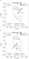 |
Fig. 5 Comparison of the theoretical semi-minor axis with the measured one. We assume a prograde (a) and retrograde (b) rotation. The theoretical value is determined from Eqs. (8) and (9). Only the prograde solution is compatible with the observational data. |
4.1 Comparison between the observed and the synthetic rotational light curves
Thanks to the extensive research conducted by our group over the past two decades (Ortiz et al. 2002; Fernández-Valenzuela et al. 2017, 2023), a total of seven rotational light curves spanning from 2001 to 2023 were compiled. To again assess the accuracy of the pole solution proposed by Fernández-Valenzuela et al. (2017) and to compare it with our synthetic light curve generation tool, we computed, for each date, the rotational light curve that our ellipsoid shape model would produce as observed from Earth with a prograde rotation period of 9.1736 h. The results are shown in Fig. D.2. Our simulations align with the observed amplitude variations over this 22-year period, confirming the compatibility of the pole solution with the observations. However, it’s worth noting that the observed light curves exhibit significant asymmetry, which becomes more pronounced as the amplitude increases. These asymmetries cannot be replicated by a symmetrical triaxial shape model.
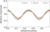 |
Fig. 6 Synthetic rotational light curve generated for Bienor as observed from Earth during Occ. A, B, and C. The light curve was sampled at intervals of 5 degrees. Animations depicting the rotation of Bienor can be accessed online. |
4.2 Overlaying chords on simulated projected ellipses
After validating the software and the rotation pole solution, we proceeded to conduct a detailed examination of the occultation on December 26, 2022, labeled as Occ. B. We assumed that Bienor was rotating around its pole in a prograde manner with a period of 9.1736 h, and the resulting backplanes and radiance were sampled with a 5-degree step. Figure 6 shows the synthetic rotational light curves for Bienor as observed from Earth during each one of the occultations presented in this work. Animations depicting the rotation of Bienor to get these light curves can be accessed through the links Occ. A, Occ. B, and Occ. C.
We projected our ellipsoid onto the sky plane at the rotational phase value calculated for this occultation (0.15), with north oriented upward along the vertical axis and east pointing to the left. Next, we also projected the chords onto the same frame and manually adjusted the angular size occupied by Bienor in that FoV to match the extremities of the chords described in Section 3.1 (see Fig. 7). The alignment agrees with that of the fitted ellipse in Fig. 2b.
Then, we replicated the process mentioned above with the chords from Occ. A and C (refer to Fig. C.1). We accounted for the geocentric distance (Δ), ensuring that the shape model projection is to scale in each case. Nearly all the chords fit well, except for the chord acquired from Van Vleck, which lies outside the projected shape of Bienor (Fig. C.1a). Since Westport observations were made with GPS (contrary to Van Vleck), we assumed that it was the Van Vleck chord that must be corrected. To estimate the temporal shift, we generated a series of solutions, from −10 to +10 s, with a step of 0.1 s, and we solved for each case, comparing the chords by superimposing them onto the projected ellipsoid shape. The best fit to the projected ellipse occurs for the chord that requires subtracting 4.0 s, and that is the chosen solution here (Fig. C.1b).
With the new refined rotation period determined in this work (9.1736 ± 0.0002 h), we computed the rotational phase of Bienor on the January 11 dip at 01:03:30.00 UT, obtaining a value of 0.67 ± 0.015 when the maximum of brightness is selected as phase 0. Then, we simulated Bienor’s shape as seen from Earth. At this time, a stellar occultation by Bienor was analyzed by Fernández-Valenzuela et al. (2023). The authors found synchronization problems between the Manzanares and Constancia chords and explored different scenarios. Knowing now the shape and orientation in the sky plane, it becomes evident that by correcting the Constancia chord, the data are consistent (see Fig. C.3).
Finally, by applying Eqs. (8) and (9), we computed the value of θν and compared it with the chords obtained in Section 3.1. Remarkably, these values also align with our simulations (see Fig. C.2).
Nevertheless, as shown in Fig. 6, this ellipsoid model cannot account for the asymmetries identified in the observational rotational light curves. The next section addresses several hypotheses that could explain the observational results.
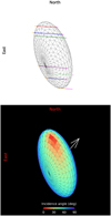 |
Fig. 7 Bienor shape model as observed from Earth during Occ. B at a rotational phase of 0.15. The top panel showcases chords from Occ. B overlaid onto the shape model, demonstrating that the shape of the projected ellipse corresponds closely to the least-squares fitted ellipse outlined in Section 3.1. The bottom panel shows the same but with coloring. The colors denote the solar incidence angle. The white arrow points toward the rotation pole. |
5 Discussion
By observing three positive occultations from Japan, Western Europe, and the USA, we have determined the shape of Bienor as a triaxial ellipsoid. We retrieved the absolute axis of the ellipsoid, and through the aspect angle and rotational phase, we theoretically computed the inclination of the minor axis of the projected ellipse onto the sky plane. This result, together with the determined ellipsoid shape, allowed us to confirm that Bienor rotates in a prograde manner. Subsequently, synthetic light curves were generated, validating the rotational phases, size, shape, and sky plane chords observed in all the stellar occultations by Bienor to date.
However, based on the assumption of a triaxial ellipsoid, our simulations predict symmetric rotational light curves. In contrast, the observed rotational curves display notable asymmetry, characterized by an absolute minimum following the absolute maximum, with a flux drop ~45% deeper than the relative one for 2023.
This discrepancy may arise from a variety of factors. A first alternative is that Bienor presents an irregular shape not detected in the occultations. Given that this is a relatively small object, likely resulting from the collision of a larger parent body, it is possible that it is an ellipsoid that can depart from hydrostatic equilibrium. To check this idea, we flattened one of Bienor’s extremities so that this deformation is not visible when Bienor is in the configuration determined for Occ. B. Then, to make the simulation more realistic, we incorporated a photometric model into our software. Unfortunately, the photometric properties of Bienor’s surface are unknown; therefore, we used the Minnaert photometric model, which only depends on a single parameter k (Minnaert 1941):
![Mathematical equation: $\[I / F=cos (i)^k ~cos (e)^{k-1}.\]$](/articles/aa/full_html/2024/09/aa50833-24/aa50833-24-eq15.png) (10)
(10)
Here, i and e are the incidence and emission angles. We verified that for different values of this parameter sufficiently high enough to break the isotropy of reflected light and account for the facets’ directionality relative to the observer, we can obtain asymmetric light curves. In Fig. D.1a, we show an illustrative result obtained for k = 2.5, with which we obtained a difference of approximately 15% between minima. Given the lack of additional data and the fact that there are infinite combinations of irregular shapes that, together with the appropriate selection of the photometric model and parameters, can reproduce asymmetries, we could not go further. Nevertheless, we confirm that this hypothesis is compatible with the observed asymmetries.
Another different idea would be to assume that Bienor is a contact binary. This is not unreasonable given that to date, we know of the existence of contact binaries in the Solar System, such as the comets 67P/Churyumov-Gerasimenko (Sierks et al. 2015) or Tuttle (Harmon et al. 2010) and the asteroids 4769 Castalia (Bottke & Melosh 1996) or 25143 Itokawa (Campo Bagatin et al. 2020), as well as TNOs, such as 486958 Arrokoth (Buie et al. 2020). These bodies are thought to have formed either through low-speed collisions during the early stages of the Solar System or through gravitational reaccumulation following catastrophic collisions. This idea is further supported by Fig. 4b, which shows an intriguing sharp dip at the minima, possibly caused by the presence of contact binaries (Showalter et al. 2021).
Nevertheless, we investigated this by creating a contact binary through the distortion of our triaxial ellipsoid, and the resulting synthetic rotational light curve lacked asymmetry (Fig. D.1b). Moreover, we found that the expected narrow brightness minima and broader maxima mentioned by (Showalter et al. 2021) are present at aspect angles close to 90 degrees. However, as the body moves away from this position, these features disappear. For Bienor, at the end of 2023 (when this light curve was taken), the aspect angle was approximately 120 degrees, so we did not expect to observe this behavior. Given that the light curve is particularly noisy during the observation of this minimum, we attribute this apparent feature to the uncertainty in these data. On the other hand, we considered the possibility that the lack of asymmetry is due to the use of a highly symmetrical shape model. To rule this out, we opted to append a smaller spherical body to the equator of the original ellipsoid, as illustrated in Fig. D.1c, thereby creating a markedly asymmetric body with a bulge at one end. However, the resulting light curve again lacked asymmetry. Then, we introduced protuberancy at a different point along the equatorial region, which, when combined with the viewing geometry, disrupted the system’s symmetry. In this scenario, the rotational light curve displayed asymmetry (Fig. D.1d), with less than a 20% difference between the minima.
In none of the above cases did we obtain values close to the ~45% measured in the real light curve. This, in addition to the absence of chords consistent with a binary system and the inability to explain the size and albedo differences when comparing to thermal measurements, led us to discard this idea as a sole explanation.
Another hypothesis for these asymmetries would be that certain regions of Bienor possess a lower albedo. There are numerous cases of objects in the Solar System, such as Earth’s moon, Iapetus, the outermost of Saturn’s large moons, or even Pluto, exhibiting clear differences in albedo on their surfaces. Another case of special interest due to its similarity is that of the TNO Haumea, a dwarf planet with the presence of water ice (Barkume et al. 2006) and an elongated shape (Ortiz et al. 2017). This object also presents an asymmetric light curve, which is thought to be due to the existence of a large surface region with an albedo and a color different from the mean surface (Lacerda et al. 2008).
For Bienor, the asymmetries appear to intensify as the object approaches a reduced aspect angle (see Fig. D.2, spanning from 2016 to 2023), indicating that this low albedo region, if present, likely resides toward the equator, making it more prominent as it is more visible. To investigate this, we conducted a simulation of a light curve using the ellipsoid shape model. For this case, we modified the software to incorporate a region centered at the equator with a lower albedo; specifically, the albedo is half that of the rest of the surface. As a result, a significant decrease in brightness (60%) is replicated (Fig. D.1e).
Finally, a last plausible explanation would be the presence of a secondary body, suggesting that the observed rotational light curve asymmetries are the result of mutual eclipses between a moon and the primary body. This rationale is further substantiated, on the one hand, by the fact that our photometric data in the visible range lead to an extrapolated area-equivalent diameter of 158 km, contrasting with the range of 179–184 km determined by Lellouch et al. (2017). Additionally, while Bienor stands out as one of the least red centaurs, with a B-V value of 1.12 ± 0.03 (Tegler et al. 2008), and previous thermal measurements indicate a geometric albedo value of ~5.0% (Bauer et al. 2013; Duffard et al. 2014a; Lellouch et al. 2017), positioning it within the dark-neutral category, our analysis revealed a higher geometric albedo of (6.5 ± 0.5)%. If the area-equivalent diameter were 170 km (instead of the 149 km determined by ellipse-fit) during the Occ. B, the geometric albedo would be ~5%. Therefore, this discrepancy in geometric albedo could also be explained by the presence of an additional object, potentially accounting for a missing reflecting area. A similar situation has been proposed for the TNO 2002 TC302 (see Ortiz et al. 2020).
To explore this scenario, we introduced a moon (same albedo as Bienor) comprising 16% of the volume of the triaxial ellipsoid, positioned at a distance 1.6 times the value of the semi-major axis a, and situated at Bienor’s equatorial plane. We performed the simulations for November 15, 2023, the date when the rotational light curve showed the greatest asymmetry. However, upon computing the reflected light across a grid of orbital phases with a 10-degree increment (defining orbital phases as the Moon-Earth-Bienor angle), the expected asymmetric light curve did not appear. This arises from the fact that the alignment of Bienor, the Sun, and the Earth does not yield mutual eclipses (primary and secondary) for a moon in an equatorial orbit under such configurations.
We then investigated this hypothesis by adjusting the inclination plane of the satellite in increments of 5 degrees, simulating light curves, and revisiting the outcomes. Certain configurations, due to the mutual eclipse events, produced asymmetric light curves (as illustrated in Fig. D.1e, exhibiting an 18% asymmetry between minima). However, achieving such asymmetric behavior necessitates that the rotational plane of the moon possess an inclination of around 125° relative to Bienor’s equatorial plane. Unfortunately, our available data are insufficient to determine the axes’ dimensions, orbital inclination, distance, or shape of this hypothetical moon. There would also be the possibility that it is not a solid object but rather a ring with a non-homogeneous density. Although no discernible drop in signal was observed in any occultation light curve, given that the S/N was not sufficiently high, we cannot dismiss the possibility of an additional companion entirely.
The observed asymmetries and discrepancies in the size estimations are sufficient evidence to support the notion of a satellite or ring’s existence while not excluding the possibility of irregularities on Bienor’s surface or variations in albedo. However, there is no data that favors or completely discards any of the hypotheses. It is even plausible that both hypotheses are simultaneously valid. Further data collection is necessary to constrain and fully understand this system.
6 Conclusions
In this work, the analysis of three positive occultations of Bienor from Japan, Western Europe, and the United States together with the rotational light curve data gathered from Spain as well as the development of a tool for generating synthetic light curves allowed us to do the following:
Determine the projected ellipse of Bienor for December 26, 2022, showing that it is compatible with the proposed semi-axis ratios of b/a = 0.45 and c/b = 0.79;
Confirm a prograde rotation of Bienor and validate that the rotational pole solution of βp = 50°, λp = 35° aligns with observations spanning 22 year;
Confirm the presence of a clear asymmetry in the rotational light curve with distinct absolute and relative minima;
Refine the rotation period of Bienor to 9.1736 ± 0.0002 hours;
Determine the absolute values of the axes of the triaxial ellipsoid: a = (127 ± 5) km, b = (55 ± 4) km, and c = (45 ± 4) km. Using these values, we compared the area-equivalent diameter with thermal estimates and found that our solution yields a lower value
Determine a geometric albedo for Bienor of (6.5 ± 0.5)%, which is higher than the geometric albedo determined previously by other methods based on thermal data;
Show through a three-dimensional simulation of the rotational light curves that a combination of shape irregularities; the presence of an additional object, such as a satellite; and significant albedo differences on the surface could explain the measured discrepancies.
Unfortunately, no occultation to date has a recorded flux measurement to constrain the problem and discard any of the hypotheses presented here. In the future, new data will eventually clarify the issue.
Movies
Download all Movies Access Supplementary Material
Movie 1 associated to Figs. 6 and D.1 (06_02_2022) Access Supplementary Material
Movie 2 associated to Figs. 6 and D.1 (14_02_2023) Access Supplementary Material
Movie 3 associated to Figs. 6 and D.1 (26_12_2022) Access Supplementary Material
Movie 4 associated to Figs. 6 and D.1 (binary) Access Supplementary Material
Movie 5 associated to Figs. 6 and D.1 (binary_asym) Access Supplementary Material
Movie 6 associated to Figs. 6 and D.1 (binary_asym2) Access Supplementary Material
Movie 7 associated to Figs. 6 and D.1 (irregular) Access Supplementary Material
Movie 8 associated to Figs. 6 and D.1 (moon) Access Supplementary Material
Movie 9 associated to Figs. 6 and D.1 (spot) Access Supplementary Material
Acknowledgements
J.L. Rizos, J.L. Ortiz, N. Morales, P. Santos-Sanz, M. Varia-Lubiano, R. Leiva, M. Kretlow, R. Morales, A. Alvarez-Candal, R. Duffard and J.M. Gómez-Limón acknowledge financial support from the Severo Ochoa grant CEX2021-001131-S funded by MCIN/AEI/10.13039/501100011033. J. L. Rizos acknowledges support from the Ministry of Science and Innovation under the funding of the European Union NextGeneration EU/PRTR. P. Santos-Sanz acknowledges financial support from the Spanish I+D+i project PID2022-139555NB-I00 (TNO-JWST) funded by MCIN/AEI/10.13039/501100011033. This work has made use of data from the European Space Agency (ESA) mission Gaia, processed by the Gaia Data Processing and Analysis Consortium (DPAC). Funding for the DPAC has been provided by national institutions, in particular the institutions participating in the Gaia Multilateral Agreement. This work is partly based on observations collected at the Centro Astronómico Hispano en Andalucía (CAHA) at Calar Alto, operated jointly by Junta de Andalucía and Consejo Superior de Investigaciones Científicas (CSIC). This research is also partially based on observations carried out at the Observatorio de Sierra Nevada (OSN) operated by Instituto de Astrofísica de Andalucía (IAA-CSIC).
Appendix A Occulted stars
Hertzsprung–Russell diagram showing the absolute magnitude versus the color index (B-V) of stars from the HYG star database archive6, which combines data from the HIP-PARCOS, Yale Bright Star, and Gliese (nearby star) catalogs. The occulted stars analyzed in Section 2 are plotted, including Occ. A (202357903847210880 - GaiaDR3) and Occ. B (961233167113907328 - GaiaDR3), which are giant stars, and Occ. C (193308850132660224 - GaiaDR3), which is a main-sequence star.
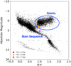 |
Fig. A.1 Absolute magnitude versus color index (B-V) of the HYG star database along with the stars occulted by Bienor and analyzed in this work. |
Appendix B Stellar occultation analyses
Light curves from the occultation events described in Section 3.1. Additionally, tables containing the ingress and egress times after the square well fits are provided, along with the expanded table containing information about the location of telescopes, instruments, and observers.
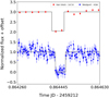 |
Fig. B.1 Normalized flux value (with offset for better visualization) obtained from the two observations made during Occ. A on February 6, 2022. The observations present a flux drop of 17.4σ for Van Vleck (red) and 4.8σ for Westport (blue). The black line represents a square well fit to the observational data. |
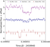 |
Fig. B.2 Normalized flux value (with offset for better visualization) obtained from the three observations made during Occ. B from Japan on December 26, 2022. The flux drop (measured in σ) appears at the top. The black line represents a square-well fit to the observational data. |
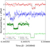 |
Fig. B.3 Normalized flux value (with offset for better visualization) obtained from the four observations made during Occ. B from Western Europe on December 26, 2022. The flux drop (measured in σ) appears at the top. The black line represents a square-well fit to the observational data. |
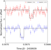 |
Fig. B.4 Normalized flux value (with offset for better visualization) obtained from the two observations made during Occ. C on February 14, 2024. They present a flux drop of 3.7σ for Cottered (red) and 4.7σ for Nandrin S.A.L (blue). The black line represents a square-well fit to the observational data. |
Observatories, instrumentation, and observers.
UT ingress and egress times and errors for each observation.
Appendix C Compatibility of chords with ellipsoidal
In this Appendix, we include the figures generated to study the compatibility of the projected chords in the sky plane with the orientation and size of the ellipsoid generated by our synthetic rotational light curve simulation software. Specifically, we include the figures of the chords superimposed on the projections of the shape model described in Section 4. In addition, we include diagrams showing the calculated position angle of the minor axis of the ellipse (Eq. 8 and 9) for Occ. A and C.
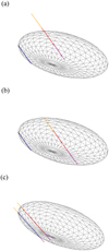 |
Fig. C.1 a) Chords from Occ. A superimposed onto the shape model, as seen from Earth (the north pointing upward and the east to the left), at a rotational phase value of 0.888. b) Same as on top but with Van Vleck’s chord shifted 4.0 seconds so that it matches the projected shape (see Section 4.2). c) Chords from Occ. C overlaid onto the shape model as seen from Earth with a rotational phase of 0.93. Geocentric distance (Δ) is taken into account so that the size of the ellipsoids are to scale. |
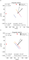 |
Fig. C.2 a) Occ. A’s chords and value of the minor axis of the ellipse, determined using Eq. 8 and 9 for the prograde rotation. b) Same for Occ. C. Both solutions are consistent with the projected ellipse in Fig. C.1. To the right of each plot is included the position angle of the rotation pole (θp), and minor axis of the projected ellipse (θv), as well as the rotational phase and aspect angles. |
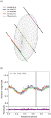 |
Fig. C.3 a) Shape model of Bienor, as seen from Earth on January 11, 2019, at 01:03:30 UT, with the chords of the occultation observed at that time and analyzed by Fernández-Valenzuela et al. (2023). The authors found synchronization issues between the Manzanares and Constancia chords. Now it becomes evident that it is the Constancia chord (red) that had to be corrected. b) Rotational light curve using observational data from 2019 as reported by Fernández-Valenzuela et al. (2023). With the newly refined period from this work, the rotational phase was 0.67 ± 0.015. Dashed lines show the uncertainty after studying how the 0.0002 h error propagates with time. A unique color represents each observation day. At the bottom, it is shown the difference (residual) between the modeled curve and the observational data. |
Appendix D Synthetic rotational light curves
In this appendix, the light curves generated through simulation software and the projections of the shape models used in this work are shown.
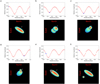 |
Fig. D.1 Simulated rotational light curves using the Minnaert photometric model (Eq. 10, k=2.5) for various configurations observed from Earth on November 15, 2023. a) LC for the determined ellipsoidal shape for Bienor, but with a flattening at one of its ends. This configuration generates an asymmetric light curve with a ~15% drop difference between minima. b) LC for a symmetric contact binary matching the dimensions of the ellipsoid shape model. No asymmetric light curve is generated. c) LC for an asymmetric contact binary, in which one of the lobes is smaller than theother.Noasymmetriclightcurveisgenerated.d)Similarto(c), where the smaller object is now shifted from the symmetry axis of the ellipsoid. In this case, the minima are different, with a ~20% difference in the drop. e) LC for an ellipsoid featuring a low-albedo region (half the regular albedo) in its equatorial area. In this example, up to 60% asymmetry between the minima is achieved. f) LC for an ellipsoid with a satellite of 16 % of its volume. This configuration, in which the orbital plane of the moon is inclined at 125° relative to the equatorial plane of Bienor (producing mutual eclipses), gives an asymmetric rotational with a difference of 18% drop between minima. An animation of each checked hypothesis can be accessed online. The white arrow points toward the rotation pole. The blue dot in the rotational light curve plots indicates the point corresponding to the image below. The colors indicate the value of the solar incidence angle, following the same scale shown in Fig. 7. |
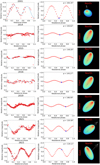 |
Fig. D.2 Left column: rotational light curves observed since 2001 (Ortiz et al. 2002; Fernández-Valenzuela et al. 2017, 2023). Julian date has been corrected for light travel time and phased using the refined period of 9.1736 h. Middle column: synthetic rotational light curves for a triaxial ellipsoid (b/a = 0.45, c/b = 0.79) using the prograde sense of rotation (Fernández-Valenzuela et al. 2017) generated by our software. At the upper right corner of each plot, the value of the aspect angle is displayed. The resulting backplanes and radiance are sampled with a 10-degree step. Right column: shape model as seen from Earth at the minimum brightness of the synthetic rotational light curve. The colors indicate the value of the solar incidence angle, following the same scale shown in Fig. 7. The white arrow points toward the rotation pole. The blue dot in the middle plots indicates the point that corresponds to the image on the right. |
References
- Barkume, K. M., Brown, M. E., & Schaller, E. L. 2006, ApJ, 640, L87 [NASA ADS] [CrossRef] [Google Scholar]
- Bauer, J. M., Choi, Y.-J., Weissman, P. R., et al. 2008, PASP, 120, 393 [Google Scholar]
- Bauer, J. M., Grav, T., Blauvelt, E., et al. 2013, ApJ, 773, 22 [Google Scholar]
- Bottke, William F. J., & Melosh, H. J. 1996, Icarus, 124, 372 [Google Scholar]
- Braga-Ribas, F., Sicardy, B., Ortiz, J. L., et al. 2014, Nature, 508, 72 [NASA ADS] [CrossRef] [Google Scholar]
- Braga-Ribas, F., Pereira, C. L., Sicardy, B., et al. 2023, A&A, 676, A72 [NASA ADS] [CrossRef] [EDP Sciences] [Google Scholar]
- Buie, M. W., Porter, S. B., Tamblyn, P., et al. 2020, AJ, 159, 130 [NASA ADS] [CrossRef] [Google Scholar]
- Campo Bagatin, A., Alemañ, R. A., Benavidez, P. G., Pérez-Molina, M., & Richardson, D. C. 2020, Icarus, 339, 113603 [NASA ADS] [CrossRef] [Google Scholar]
- Collins, K. A., Kielkopf, J. F., Stassun, K. G., & Hessman, F. V. 2017, AJ, 153, 77 [Google Scholar]
- DeMeo, F. E., Fornasier, S., Barucci, M. A., et al. 2009, A&A, 493, 283 [NASA ADS] [CrossRef] [EDP Sciences] [Google Scholar]
- Desmars, J., Camargo, J. I. B., Braga-Ribas, F., et al. 2015, A&A, 584, A96 [NASA ADS] [CrossRef] [EDP Sciences] [Google Scholar]
- Di Sisto, R. P., & Brunini, A. 2007, Icarus, 190, 224 [Google Scholar]
- Dotto, E., Barucci, M. A., Boehnhardt, H., et al. 2003, Icarus, 162, 408 [NASA ADS] [CrossRef] [Google Scholar]
- Duffard, R., Pinilla-Alonso, N., Ortiz, J. L., et al. 2014a, A&A, 568, A79 [NASA ADS] [CrossRef] [EDP Sciences] [Google Scholar]
- Duffard, R., Pinilla-Alonso, N., Santos-Sanz, P., et al. 2014b, A&A, 564, A92 [NASA ADS] [CrossRef] [EDP Sciences] [Google Scholar]
- Duncan, M. J., & Levison, H. F. 1997, Science, 276, 1670 [Google Scholar]
- Duncan, M. J., Levison, H. F., & Budd, S. M. 1995, AJ, 110, 3073 [NASA ADS] [CrossRef] [Google Scholar]
- Durech, J., Sidorin, V., & Kaasalainen, M. 2010, A&A, 513, A46 [NASA ADS] [CrossRef] [EDP Sciences] [Google Scholar]
- Elliot, J. L., Kern, S. D., Clancy, K. B., et al. 2005, AJ, 129, 1117 [NASA ADS] [CrossRef] [Google Scholar]
- Fernández-Valenzuela, E., Ortiz, J. L., Duffard, R., Morales, N., & Santos-Sanz, P. 2017, MNRAS, 466, 4147 [NASA ADS] [Google Scholar]
- Fernández-Valenzuela, E., Morales, N., Vara-Lubiano, M., et al. 2023, A&A, 669, A112 [NASA ADS] [CrossRef] [EDP Sciences] [Google Scholar]
- Guilbert, A., Alvarez-Candal, A., Merlin, F., et al. 2009, Icarus, 201, 272 [NASA ADS] [CrossRef] [Google Scholar]
- Halíř, R., & Flusser, J. 1998, in International Conference in Central Europe on Computer Graphics and Visualization, https://autotrace.sourceforge.net/WSCG98.pdf [Google Scholar]
- Harmon, J. K., Nolan, M. C., Giorgini, J. D., & Howell, E. S. 2010, Icarus, 207, 499 [CrossRef] [Google Scholar]
- Harris, A. W., Young, J. W., Scaltriti, F., & Zappala, V. 1984, Icarus, 57, 251 [NASA ADS] [CrossRef] [Google Scholar]
- Holman, M. J., & Wisdom, J. 1993, AJ, 105, 1987 [NASA ADS] [CrossRef] [Google Scholar]
- Horner, J., Evans, N. W., & Bailey, M. E. 2004, MNRAS, 354, 798 [NASA ADS] [CrossRef] [Google Scholar]
- Hunter, J. D. 2007, Comput. Sci. Eng., 9, 90 [NASA ADS] [CrossRef] [Google Scholar]
- Kilic, Y., Braga-Ribas, F., Kaplan, M., et al. 2022, MNRAS, 515, 1346 [NASA ADS] [CrossRef] [Google Scholar]
- Lacerda, P., Jewitt, D., & Peixinho, N. 2008, AJ, 135, 1749 [CrossRef] [Google Scholar]
- Lacerda, P., Fornasier, S., Lellouch, E., et al. 2014, ApJ, 793, L2 [NASA ADS] [CrossRef] [Google Scholar]
- Leiva, R., Sicardy, B., Camargo, J. I. B., et al. 2017, AJ, 154, 159 [NASA ADS] [CrossRef] [Google Scholar]
- Lellouch, E., Moreno, R., Müller, T., et al. 2017, A&A, 608, A45 [NASA ADS] [CrossRef] [EDP Sciences] [Google Scholar]
- Lomb, N. R. 1976, Ap&SS, 39, 447 [Google Scholar]
- Magnusson, P. 1986, Icarus, 68, 1 [NASA ADS] [CrossRef] [Google Scholar]
- Masiero, J. R., Wright, E. L., & Mainzer, A. K. 2021, PSJ, 2, 32 [NASA ADS] [Google Scholar]
- Minnaert, M. 1941, ApJ, 93, 403 [Google Scholar]
- Morgado, B. E., Sicardy, B., Braga-Ribas, F., et al. 2021, A&A, 652, A141 [NASA ADS] [CrossRef] [EDP Sciences] [Google Scholar]
- Müller, T., Lellouch, E., & Fornasier, S. 2020, in The Trans-Neptunian Solar System, eds. D. Prialnik, M. A. Barucci, & L. Young (Elsevier), 153 [Google Scholar]
- Ortiz, J. L., Baumont, S., Gutiérrez, P. J., & Roos-Serote, M. 2002, A&A, 388, 661 [NASA ADS] [CrossRef] [EDP Sciences] [Google Scholar]
- Ortiz, J. L., Duffard, R., Pinilla-Alonso, N., et al. 2015, A&A, 576, A18 [NASA ADS] [CrossRef] [EDP Sciences] [Google Scholar]
- Ortiz, J. L., Santos-Sanz, P., Sicardy, B., et al. 2017, Nature, 550, 219 [NASA ADS] [CrossRef] [Google Scholar]
- Ortiz, J. L., Santos-Sanz, P., Sicardy, B., et al. 2020, A&A, 639, A134 [NASA ADS] [CrossRef] [EDP Sciences] [Google Scholar]
- Ortiz, J. L., Pereira, C. L., Sicardy, B., et al. 2023, A&A, 676, A12 [Google Scholar]
- Ostro, S. J., Connelly, R., & Dorogi, M. 1988, Icarus, 75, 30 [NASA ADS] [CrossRef] [Google Scholar]
- Pereira, C. L., Braga-Ribas, F., Sicardy, B., et al. 2024, MNRAS, 527, 3624 [Google Scholar]
- Press, W. H., Teukolsky, S. A., Vetterling, W. T., & Flannery, B. P. 1992, Numerical Recipes in FORTRAN. The Art of Scientific Computing (Cambridge University Press) [Google Scholar]
- Rousselot, P., Kryszczyńska, A., Bartczak, P., et al. 2021, MNRAS, 507, 3444 [NASA ADS] [CrossRef] [Google Scholar]
- Russell, H. N. 1916, ApJ, 43, 173 [Google Scholar]
- Santos-Sanz, P., Ortiz, J. L., Sicardy, B., et al. 2021, MNRAS, 501, 6062 [NASA ADS] [CrossRef] [Google Scholar]
- Showalter, M. R., Benecchi, S. D., Buie, M. W., et al. 2021, Icarus, 356, 114098 [NASA ADS] [CrossRef] [Google Scholar]
- Sierks, H., Barbieri, C., Lamy, P. L., et al. 2015, Science, 347, aaa1044 [Google Scholar]
- Strauss, R. H., Leiva, R., Keller, J. M., et al. 2021, PSJ, 2, 22 [NASA ADS] [Google Scholar]
- Tegler, S. C., Bauer, J. M., Romanishin, W., & Peixinho, N. 2008, in The Solar System Beyond Neptune, eds. M. A. Barucci, H. Boehnhardt, D. P. Cruikshank, A. Morbidelli, & R. Dotson (University of Arizona Press), 105 [Google Scholar]
- Tegler, S. C., Romanishin, W., Consolmagno, G. J., & J., S. 2016, AJ, 152, 210 [NASA ADS] [CrossRef] [Google Scholar]
- van Belle, G. T. 1999, PASP, 111, 1515 [NASA ADS] [CrossRef] [Google Scholar]
- Zacharias, N., Monet, D. G., Levine, S. E., et al. 2004, AAS Meet. Abstr. 205, 48.15 [NASA ADS] [Google Scholar]
At the time of writing this article, 761 centaurs are listed at https://ssd.jpl.nasa.gov/
All Tables
Bienor aspect angle (ψ) and position angle of the rotation pole (θp) for prograde (1) and retrograde (2) solutions.
All Figures
|
Fig. 1 Predicted occultation shadow path computed for February 6, 2022 (a), December 26, 2022 (b & c), and February 14, 2023 (d). Green lines depict the boundaries of the shadow paths, while the gray lines represent the uncertainty in the path resulting from orbital uncertainties. A red line denotes the center of the shadow path, and the pins indicate the positions of the stations involved in the campaigns. Green pins signify sites where a positive occultation was observed. The maps were generated using OpenStreetMap via the Occultation Portal. The dotted arrow denotes the shadow’s direction of motion. |
| In the text | |
|
Fig. 2 Chords of the stellar occultations projected on the sky plane. The ingress uncertainties are shown in pink, and the egress uncertainties are in orange. The values in parenthesis are the lengths of the chords. (a) Occ. A on February 6, 2022. The minimum distance between the chords is 71.49 km. (b) Occ. B on December 26, 2022. The dashed line describes the ellipse that best fits the points. (c) Occ. C on February 14, 2023. The minimum distance between the chords is 15.35 km. The dashed arrow in the upper-right corner indicates the direction of the shadow motion. |
| In the text | |
|
Fig. 3 Lomb periodogram’s spectral power obtained from photometric data collected in 2021 and 2023. There are two possible solutions that are very close in spectral power. The solution that best fits with the 2021 and 2023 rotational light curves is the one marked in red, (9.1736 ± 0.0002) h. |
| In the text | |
|
Fig. 4 Rotational light curves of Bienor. In (a), we present the rotational light curve using 2021 data, while (b) shows the 2023 observational data. The vertical line indicates the rotational phase during Occ. A, B, and C, respectively. In both panels, the dashed lines show the uncertainty after studying how the 0.0002 h error propagates with time. A unique color represents each observation day. At the bottom, the difference (residual) between the modeled curve and the observational data is shown. |
| In the text | |
|
Fig. 5 Comparison of the theoretical semi-minor axis with the measured one. We assume a prograde (a) and retrograde (b) rotation. The theoretical value is determined from Eqs. (8) and (9). Only the prograde solution is compatible with the observational data. |
| In the text | |
|
Fig. 6 Synthetic rotational light curve generated for Bienor as observed from Earth during Occ. A, B, and C. The light curve was sampled at intervals of 5 degrees. Animations depicting the rotation of Bienor can be accessed online. |
| In the text | |
|
Fig. 7 Bienor shape model as observed from Earth during Occ. B at a rotational phase of 0.15. The top panel showcases chords from Occ. B overlaid onto the shape model, demonstrating that the shape of the projected ellipse corresponds closely to the least-squares fitted ellipse outlined in Section 3.1. The bottom panel shows the same but with coloring. The colors denote the solar incidence angle. The white arrow points toward the rotation pole. |
| In the text | |
|
Fig. A.1 Absolute magnitude versus color index (B-V) of the HYG star database along with the stars occulted by Bienor and analyzed in this work. |
| In the text | |
|
Fig. B.1 Normalized flux value (with offset for better visualization) obtained from the two observations made during Occ. A on February 6, 2022. The observations present a flux drop of 17.4σ for Van Vleck (red) and 4.8σ for Westport (blue). The black line represents a square well fit to the observational data. |
| In the text | |
|
Fig. B.2 Normalized flux value (with offset for better visualization) obtained from the three observations made during Occ. B from Japan on December 26, 2022. The flux drop (measured in σ) appears at the top. The black line represents a square-well fit to the observational data. |
| In the text | |
|
Fig. B.3 Normalized flux value (with offset for better visualization) obtained from the four observations made during Occ. B from Western Europe on December 26, 2022. The flux drop (measured in σ) appears at the top. The black line represents a square-well fit to the observational data. |
| In the text | |
|
Fig. B.4 Normalized flux value (with offset for better visualization) obtained from the two observations made during Occ. C on February 14, 2024. They present a flux drop of 3.7σ for Cottered (red) and 4.7σ for Nandrin S.A.L (blue). The black line represents a square-well fit to the observational data. |
| In the text | |
|
Fig. C.1 a) Chords from Occ. A superimposed onto the shape model, as seen from Earth (the north pointing upward and the east to the left), at a rotational phase value of 0.888. b) Same as on top but with Van Vleck’s chord shifted 4.0 seconds so that it matches the projected shape (see Section 4.2). c) Chords from Occ. C overlaid onto the shape model as seen from Earth with a rotational phase of 0.93. Geocentric distance (Δ) is taken into account so that the size of the ellipsoids are to scale. |
| In the text | |
|
Fig. C.2 a) Occ. A’s chords and value of the minor axis of the ellipse, determined using Eq. 8 and 9 for the prograde rotation. b) Same for Occ. C. Both solutions are consistent with the projected ellipse in Fig. C.1. To the right of each plot is included the position angle of the rotation pole (θp), and minor axis of the projected ellipse (θv), as well as the rotational phase and aspect angles. |
| In the text | |
|
Fig. C.3 a) Shape model of Bienor, as seen from Earth on January 11, 2019, at 01:03:30 UT, with the chords of the occultation observed at that time and analyzed by Fernández-Valenzuela et al. (2023). The authors found synchronization issues between the Manzanares and Constancia chords. Now it becomes evident that it is the Constancia chord (red) that had to be corrected. b) Rotational light curve using observational data from 2019 as reported by Fernández-Valenzuela et al. (2023). With the newly refined period from this work, the rotational phase was 0.67 ± 0.015. Dashed lines show the uncertainty after studying how the 0.0002 h error propagates with time. A unique color represents each observation day. At the bottom, it is shown the difference (residual) between the modeled curve and the observational data. |
| In the text | |
|
Fig. D.1 Simulated rotational light curves using the Minnaert photometric model (Eq. 10, k=2.5) for various configurations observed from Earth on November 15, 2023. a) LC for the determined ellipsoidal shape for Bienor, but with a flattening at one of its ends. This configuration generates an asymmetric light curve with a ~15% drop difference between minima. b) LC for a symmetric contact binary matching the dimensions of the ellipsoid shape model. No asymmetric light curve is generated. c) LC for an asymmetric contact binary, in which one of the lobes is smaller than theother.Noasymmetriclightcurveisgenerated.d)Similarto(c), where the smaller object is now shifted from the symmetry axis of the ellipsoid. In this case, the minima are different, with a ~20% difference in the drop. e) LC for an ellipsoid featuring a low-albedo region (half the regular albedo) in its equatorial area. In this example, up to 60% asymmetry between the minima is achieved. f) LC for an ellipsoid with a satellite of 16 % of its volume. This configuration, in which the orbital plane of the moon is inclined at 125° relative to the equatorial plane of Bienor (producing mutual eclipses), gives an asymmetric rotational with a difference of 18% drop between minima. An animation of each checked hypothesis can be accessed online. The white arrow points toward the rotation pole. The blue dot in the rotational light curve plots indicates the point corresponding to the image below. The colors indicate the value of the solar incidence angle, following the same scale shown in Fig. 7. |
| In the text | |
|
Fig. D.2 Left column: rotational light curves observed since 2001 (Ortiz et al. 2002; Fernández-Valenzuela et al. 2017, 2023). Julian date has been corrected for light travel time and phased using the refined period of 9.1736 h. Middle column: synthetic rotational light curves for a triaxial ellipsoid (b/a = 0.45, c/b = 0.79) using the prograde sense of rotation (Fernández-Valenzuela et al. 2017) generated by our software. At the upper right corner of each plot, the value of the aspect angle is displayed. The resulting backplanes and radiance are sampled with a 10-degree step. Right column: shape model as seen from Earth at the minimum brightness of the synthetic rotational light curve. The colors indicate the value of the solar incidence angle, following the same scale shown in Fig. 7. The white arrow points toward the rotation pole. The blue dot in the middle plots indicates the point that corresponds to the image on the right. |
| In the text | |
Current usage metrics show cumulative count of Article Views (full-text article views including HTML views, PDF and ePub downloads, according to the available data) and Abstracts Views on Vision4Press platform.
Data correspond to usage on the plateform after 2015. The current usage metrics is available 48-96 hours after online publication and is updated daily on week days.
Initial download of the metrics may take a while.