| Issue |
A&A
Volume 697, May 2025
|
|
|---|---|---|
| Article Number | A62 | |
| Number of page(s) | 16 | |
| Section | Planets, planetary systems, and small bodies | |
| DOI | https://doi.org/10.1051/0004-6361/202554154 | |
| Published online | 07 May 2025 | |
The trans-Neptunian object (119951) 2002 KX14 revealed via multiple stellar occultations
1
Instituto de Astrofísica de Andalucía – Consejo Superior de Investigaciones Científicas (IAA-CSIC),
Glorieta de la Astronomía S/N,
18008
Granada,
Spain
2
Florida Space Institute,
12354 Research Parkway, Partnership I, Room 211,
32826
Orlando,
USA
3
Federal University of Technology - Paraná (UTFPR/PPGFA),
Av. Sete de Setembro, 3165,
CEP 80230-901 - Curitiba - PR - Brazil
4
Laboratório Interinstitucional de e-Astronomia (LIneA/INCT do e-Universo),
Av. Pastor Martin Luther King Jr, 126,
20765
Rio de Janerio,
Brazil
5
LTE, Observatoire de Paris, Université PSL, Sorbonne Université, Université de Lille, LNE,CNRS 61 Avenue de l’Observatoire,
75014
Paris,
France
6
Institut Polytechnique des Sciences Avancées IPSA,
63 boulevard de Brandebourg,
94200
Ivry-sur-Seine,
France
7
LIRA, CNRS UMR-8254, Observatoire de Paris, Université PSL, Sorbonne Université, Université Paris Cité, CY Cergy Paris Université,
Meudon
92190,
France
8
Space Telescope Science Institute,
3700 San Martin Drive,
Baltimore,
USA
9
Astronomical Observatory Institute, Faculty of Physics and Astronomy, Adam Mickiewicz University,
Słoneczna 36,
60-286
Poznań,
Poland
10
Astronomical Observatory of Odesa I.I. Mechnikov National University,
1v Marazliivska str.,
Odesa
65014,
Ukraine
11
Konkoly Observatory,
Budapest,
Hungary
12
ELTE Eötvös Loránd University, Gothard Astrophysical Observatory,
Szent Imre h u 112,
Szombathely,
Hungary
13
Maastricht University, Maastricht Science Programme,
Maastricht,
The Netherlands
14
Observatoire de Nandrin, Société Astronomique de Liège, Belgium
15
Institute of Planetary Research, DLR,
Rutherfordstr. 2,
12489
Berlin,
Germany
16
Centro de Estudios de Física del Cosmos de Aragón,
Plaza de San Juan, 1,
44001
Teruel,
Spain
17
La Hita Observatory,
Toledo,
Spain
18
International Occultation Timing Association (IOTA), USA
19
Department of Astronomy, University of Virginia,
Charlottesville, VA,
USA
20
New Mexico State University - Apache Point Observatory, USA
21
GOA, UFES,
Av. Fernando FErrari, 514 Vitória, ES,
Brazil
22
Sonear3 Observatory, USA
23
DogsHeaven Observatory,
Brasília,
Brazil
24
Botorrita Observatory,
Botorrita,
Spain
25
Universidade Federal do Rio de Janeiro - Observatório do Valongo,
Ladeira Pedro Antônio 43,
CEP 20.080-090
Rio de Janeiro,
Brazil
26
Observatório Nacional,
Rua Gal. José Cristino 77,
Rio de Janeiro
RJ-20921-400,
Brazil
27
Space Science and Solar Energy Research and Application Center (UZAYMER), University of Çukurova,
Adana
01330,
Türkiye
28
Mesopotamia Astronomy Association,
Batman
72040,
Türkiye
29
Yuregir Science Center Adana
01260,
Türkiye
30
National Observatories of Türkiye, TUG,
07058
Antalya,
Türkiye
31
TÜBİTAK,
Tunus Cad., No:80,
06680
Kavaklıdere, Ankara,
Türkiye
32
Department of Space Sciences and Technologies, Akdeniz University,
Campus, Antalya
07058,
Türkiye
33
Buelach Observatory,
Bülach,
Switzerland
34
IOTA/ES, International Occultation Timing Association/European Section e.V.,
Am Brombeerhag 13,
30459
Hannover,
Germany
35
Czech Astronomical Society,
Fričova 298,
251 65
Ondřejov,
Czech Republic
36
Observatory in Rokycany and Pilsen, p.o.,
Voldušská 721,
337 01
Rokycany,
Czech Republic
37
naXys, Department of Mathematics, University of Namur,
Rue de Bruxelles 61,
Namur
5000,
Belgium
38
Institute of Physics, Federal University of Uberlândia,
Av. João Naves de Ávila,
Uberlândia, Minas Gerais
CEP 38408-100,
Brazil
★ Corresponding author: This email address is being protected from spambots. You need JavaScript enabled to view it.
Received:
17
February
2025
Accepted:
24
March
2025
Abstract
Context. Trans-Neptunian objects (TNOs) are icy bodies located in the outer solar system that offer key insights into the primordial conditions of our planetary system. The stellar occultation technique has proven to be an essential tool for studying these distant and faint objects, enabling precise determinations of their size, shape, and albedo, while also improving estimates of their orbital parameters. Among them, (119951) 2002 KX14 is a large classical TNO with limited previous observations and unresolved questions regarding its physical properties.
Aims. This study aims to analyze and characterize the TNO (119951) 2002 KX14 through observations of stellar occultations, providing unique measurements of its size, shape, and albedo. Shape measurements are especially relevant, as only thirteen TNOs have had their projected shapes measured. These results contribute to our understanding of the physical properties of this object and the broader TNO population.
Methods. Five stellar occultations by 2002 KX14 were observed from 2020 to 2023, involving multiple telescopes across different locations in Europe and the Americas. High-precision astrometry and photometric data were used to predict the occultation paths and extract ingress and egress timings. One of the events was detected from six sites and there are also several close misses, providing precise constraints for an accurate determination of the object’s limb. Furthermore, elliptical fits to the occultations chords allowed for the determination of the object’s shape and area-equivalent diameter. The geometric albedo was calculated by combining the occultation results with published absolute magnitudes.
Results. The five occultations resulted in 15 positive chords that allowed us to accurately measure the shape and size of 2002 KX14. Given that the rotational variability of this body is minimal, we can reasonably assume that the variations are due to albedo features, since the body is classed as a Maclaurin spheroid. The projected ellipse has semi-major and semi-minor axes of 241.0 ± 7.2 km and 157.1 ± 5.2 km, respectively, corresponding to an average area-equivalent diameter of 389.2 ± 8.7 km. The geometric albedo was estimated to be 11.9 ± 0.7%. These values differ from the 455 ± 27 km diameter and the 9.7-1.3+1.4% albedo derived from thermal measurements, offering a more refined understanding of the object’s physical properties.
Key words: Kuiper belt: general / Kuiper belt objects: individual: (119951) 2002 KX14
© The Authors 2025
 Open Access article, published by EDP Sciences, under the terms of the Creative Commons Attribution License (https://creativecommons.org/licenses/by/4.0), which permits unrestricted use, distribution, and reproduction in any medium, provided the original work is properly cited.
This article is published in open access under the Subscribe to Open model. This email address is being protected from spambots. You need JavaScript enabled to view it. to support open access publication.
1 Introduction
Beyond Neptune there lies a vast and diverse population of transNeptunian objects (TNOs)1, which can be dynamically classified into several groups based on their orbital characteristics (Gladman et al. 2008). On the one hand, resonant objects, such as Plutinos, are in a 3:2 resonance with Neptune and follow predictable orbital patterns influenced by the planet’s gravity. On the other hand, the classical belt (nonresonants), is divided into a “cold population”, with low inclinations and nearly circular orbits, and a “hot population”, with higher inclinations and eccentricities. Beyond this lies the scattered disk, containing objects with highly eccentric and inclined orbits that are thought to have been dynamically perturbed by Neptune. Further out, detached objects such as Sedna have perihelia that are far from Neptune’s influence, while some may represent the transition to the hypothesized inner Oort cloud.
The remote location of these icy bodies, which shields them from the intense solar radiation that affects objects closer to the Sun, makes them valuable objects for studies of the early physical and dynamical conditions that shaped our planetary system. However, it is challenging given their relatively small size (the largest TNO is Pluto, with a radius of 1188 km (Nimmo et al. 2017)), along with their low brightness and large heliocentric distances. Moreover, the low surface temperatures of TNOs (30–50 K, e.g. Stern & Trafton 2008) cause their thermal emission to peak in the far-infrared (FIR) region of the electromagnetic spectrum, which is blocked by Earth’s atmosphere. This makes space-based observations essential for their study. However, the stellar occultation technique enables ground-based observations and has proven to be one of the most effective methods for studying TNOs to date. This technique has significantly advanced our understanding of these distant icy objects by allowing for highly accurate size measurements, revealing the presence of atmospheres, moons, or rings. In addition, when combined with independent datasets, it helps determine their geometric albedo (e.g. Hubbard et al. 1988; Sicardy et al. 2011; Ortiz et al. 2017; Assafin et al. 2023). Moreover, it achieves kilometric precision, making it especially useful for refining the orbital parameters through astrometry and making highly accurate shape determinations.
In this work, we focus on the trans-Neptunian object (119951) 2002 KX14, discovered in 2002, which has a semi-major axis of 38.63 au, an eccentricity of 0.04, and an inclination of 0.41°. This object exhibits orbital characteristics; specifically, low eccentricity and low inclination, which are typical of the cold classical population. Members of this population are the most dynamically stable objects in the classical belt and are believed to have formed in situ, making them valuable tracers of the early formation history of the trans-Neptunian region (Delsanti & Jewitt 2006). However, the semi-major axis of 2002 KX14 places it outside the classical belt region, which is generally defined between ~42 and 47 au. Some authors (e.g., Fernández-Valenzuela et al. 2021) have classified it as an inner classical object, a population that is not considered to be an extension of the cold classicals, but instead belonging to the low-inclination tail of the hot population (Vilenius et al. 2012). Unlike the cold classicals, the hot population is thought to have been dynamically excited and relocated to its current position during the migration of the giant planets. During this migration, gravitational interactions perturbed their orbits, increasing both their inclination and eccentricity. Therefore, studying 2002 KX14 is particularly valuable because its orbital properties place it near the boundary between the cold and hot classical populations, offering insights into the dynamical structure and evolutionary history of the trans-Neptunian region.
Based on thermal measurements with the Herschel Space Telescope, Vilenius et al. (2012) estimated a diameter of 455 ± 27 km and a geometric albedo (pV) of  . This diameter is close to the size where hydrostatic equilibrium may no longer be maintained (Tancredi & Favre 2008). Subsequent ground-based observations studied its photometric properties, providing values of its absolute magnitude in the R-band: HR = 4.349 ± 0.124 (Peixinho et al. 2012), HR = 4.46 ± 0.01 (Benecchi & Sheppard 2013), and in the V-band: HV = 5.07 ± 0.03 (Boehnhardt et al. 2014), HV = 4.978 ± 0.017 (AlvarezCandal et al. 2016). Also, Alvarez-Candal et al. (2014) recorded a positive occultation, measuring a chord of 415 ± 1 km and retrieving an equivalent diameter of
  . Subsequently, Rommel et al. (2020) obtained two additional chords of 421 ± 3 km and 431 ± 6 km. Despite these successful observations, due to its faint apparent magnitude above 20.5 in the V-band, with rotational variations under 0.05 mag (Benecchi & Sheppard 2013), the shape of 2002 KX14 as well as its pole and rotation period are unknown.
In this study, we present the results of five positive occultations, which yield a total of 15 chords on five different dates. These observations have allowed us to determine the object’s shape and geometric albedo. Currently, only thirteen TNOs have projected shape determinations (Ortiz et al. 2012; BenedettiRossi et al. 2016; Ortiz et al. 2017; Dias-Oliveira et al. 2017; Benedetti-Rossi et al. 2019; Ortiz et al. 2020; Souami et al. 2020; Santos-Sanz et al. 2022; Vara-Lubiano et al. 2022; Pereira et al. 2023; Rommel et al. 2023; Kretlow et al. 2024), with 2002 KX14 being now the first2 cold classical object (if confirmed). The fact that it is close to the critical diameter beyond which hydrostatic equilibrium may no longer be maintained makes determining its shape a particularly interesting undertaking. Therefore, this study is poised to contribute to the growing body of knowledge on TNOs, laying the groundwork for future in-depth studies, providing data to enhance the statistics that allow us to contextualize this population more comprehensively, and demonstrating the effectiveness of the occultation technique in characterizing these distant objects.
2 Observations
Initial predictions for 2002 KX14 were made using the Numerical Integration of the Motion of an Asteroid (NIMA) solution (Desmars et al. 2015). Subsequently, several observational campaigns were conducted prior to each occultation using the 1.23 m telescope at the Calar Alto Observatory and the 2.0 m Liverpool Telescope located at the Roque de los Muchachos Observatory. These efforts were aimed at performing astrometry for this TNO and refining the predicted occultation shadow path, which was communicated to observers for proper deployment, in cases where mobile equipment was used. This approach enabled the observation of five positive occultations in 2020, 2022, and 2023, as described in the following sections.
2.1 Occultation A: May 26, 2020
On May 26, 2020, an occultation by 2002 KX14 of the star Gaia DR3 4111560308371475840 (see Table 1) was predicted to happen at 22:29:12 UT (referred to hereafter as “Occ. A”).
The event was observed from nine different locations, resulting in six positive detections from Borowiec (Poland), OdesaMayaki Observatory (Ukraine), Konkoly Observatory (Hungary), Gothard Astrophysical Observatory (Hungary), MillenBruch (Germany), and Nandrin (Belgium); and two negative detections: from Buelach (Switzerland) and Çukurova (Turkey). In addition, it was also observed from Tubitak Observatory (Turkey) and Marseilles (France), but the signal-to-noise ratio (S/N) of the data was too low to confirm whether the occultation occurred or not. An additional positive detection was obtained from Strasice (Czechia), but due to technical issues with the data format, it was not possible to determine the ingress and egress times with sufficient accuracy to be useful for this work. Fig. A.2a shows the predicted occultation shadow path along with the position of the observing stations involved in this work. Table B.1 expands on the information regarding locations, instrumentation, and the observers involved. Time series observations were obtained and time synchronized using Network Time Protocol (NTP) servers or global positioning systems (GPS) devices. Image acquisition started at least ∼5 min before and ended ~ 5 min after the occultation time. No filters were used to maximize the S/N of the occulted star.
The angular diameter of the occulted star was estimated using the following equation (van Belle 1999):
 (1)
(1)
as it is a giant star (see the Hertzsprung–Russell diagram in Fig. A.1) (a, b) = (0.669, 0.223) according to van Belle (1999). V and K denote the apparent magnitudes of the star in the V-band and K-band, being V = 14.750 mag and K = 10.520 mag (Zacharias et al. 2004). Consequently, the angular diameter is calculated as 0.046 mas, corresponding to 1.26 km at a 2002 KX14’s geocentric distance (Δ) of 38.01 au. As the central wavelength (λ) is ~600 nm for our CCD/CMOS observations, using Eq. (2), the Fresnel scale of this object can be calculated as 1.3 km,
 (2)
(2)
The minimum cycle time (exposure plus read-out time) here comes from the observations made in Gothard Observatory and Millen-Bruch, which was recorded at 0.7 seconds. With 2002 KX14’s velocity at the time of occultation measured at 23.41 km/s, this cycle time corresponds to a distance of 16.38 km. Given that this distance is an order of magnitude larger than that derived from the star’s angular size and Fresnel diffraction effects, they have a small impact on the derivation of ingress and egress times. Nevertheless, they were taken into account.
Occulted stars by 2002 KX14 presented in this work.
2.2 Occultation B: June 23, 2022
On June 23, 2022, an occultation of the star Gaia DR3 4116601049409385472 by 2002 KX14 (Table 1), with a predicted maximum duration of 18.7 seconds, was forecasted to occur at 00:51:33 UT (hereafter, “Occ. B”). The event was observed from four locations in Spain: the Botorrita, Javalambre, La Hita, and Calar Alto observatories. Three of these observatories, Javalambre, La Hita, and Calar Alto, reported positive detections, while Botorrita experienced technical issues (Fig. A.2b, Table B.1). Time series observations were captured and synchronized using either NTP servers or GPS devices. Image acquisition started approximately ~5 minutes before and concluded ~5 minutes after the predicted event time. No filters were applied to optimize the S/N of the star.
The angular diameter of the occulted star was estimated to be 0.019 mas using Eq. (1) (giant star, see Fig. A.1), with magnitudes of V = 17.78 and K = 12.31 mag from Zacharias et al. (2004); Lasker et al. (2008). At 2002 KX14’s geocentric distance of Δ = 37.88 au, this corresponds to a physical diameter of 0.58 km. The Fresnel scale in this case is 1.3 km. Given that the minimum observation cycle time was 1.5 seconds and 2002 KX14’s velocity during the occultation was 24.33 km/s, this timing corresponds to a distance of 36.49 km. Thus, the ingress and egress determination uncertainty mainly comes the photometric accuracy of the occultation light curves. Still, the star’s angular size and Fresnel diffraction effects were included in the analysis.
2.3 Occultation C: May 17, 2023
On May 17, 2023, an occultation by 2002 KX14 of the star Gaia DR3 4068746489444765440 (Table 1) with a maximum duration of 22.3 seconds was predicted at 08:51:46 UT (referred to hereafter as “Occ. C”). The star was observed from three telescopes, resulting in all cases with positive detections. The telescopes were located in Shiawassee, Comer Field and Nederland, USA (Fig. A.2c, Table B.1). Time series observations were obtained and synchronized using GPS devices. Image acquisition started at least ~5 min before and ended 5 min later than the predicted time. No filters were used to maximize the S/N of the star.
An angular diameter of 0.046 mas of the occulted star was estimated using Eq. (1) (giant star, see Fig. A.1), with V = 16.47 mag and K = 10.71 mag from Zacharias et al. (2004). This corresponds to 1.25 km at 2002 KX14’s geocentric distance, Δ, of 37.97 au. The Fresnel scale in this case is 1.3 km. Because the minimum cycle time for these observations is 2.0 seconds, while 2002 KX14’s velocity at the time of occultation was 20.38 km/s, it translates to a distance of 40.76 km. Given that this distance is orders of magnitude greater than that derived from the star’s angular size and Fresnel diffraction effects, the stellar angular size and diffraction have a slight impact on the derivation of ingress and egress times. However, they were accounted for.
2.4 Occultation D: May 19, 2023
Two days later, on May 19, 2023, an occultation by 2002 KX14 of the star Gaia DR3 4068793394867887872 (Table 1) with a maximum duration of 21.8 seconds was predicted to happen at 03:08:49 UT (hereafter “Occ. D”). Observations of this event were conducted from three locations in Brazil, with positive detections reported by the GOA and Sonear3 observatories; whereas in DogsHeaven, the S/N of the data was too low (Fig. A.2d, Table B.1). Time series data were collected and synchronized using NTP servers. The image capture began approximately ~5 min before the event and continued for about five minutes afterward. To maximize the star’s S/N, no filters were applied.
Using Eq. (1) (giant star; see Fig. A.1), the occulted star’s diameter was estimated to be 0.032 mas, with magnitudes of V = 16.39 mag and K = 11.36 mag from Zacharias et al. (2004). At 2002 KX14’s geocentric distance of 37.96 au, this angular size corresponds to a physical diameter of 0.89 km. The Fresnel scale is again 1.3 km. Given that the minimum observation cycle time is 6.8 seconds and that 2002 KX14’s velocity during the occultation was 20.83 km/s, this timing translates to a spatial distance of 141.64 km. Thus, the ingress and egress determination uncertainty mainly comes from the photometric accuracy of the occultation light curves. Even so, the star’s angular size and Fresnel diffraction effects were included in the analysis.
2.5 Occultation E: July 01, 2023
On July 01, 2023, the last occultation occultation by 2002 KX14 of the star Gaia DR3 4116448256084153472 (Table 1), with a maximum duration of 19.2 seconds, was predicted to occur at 07:09:22 UT (referred to hereafter as “Occ. E”). The star was observed from a single telescope, which resulted in a positive detection. The telescope was located in the Sacramento Mountains, New Mexico, USA (Fig. A.2e, Table B.1). Timeseries observations were obtained and synchronized using GPS devices. Image acquisition started at least 5 minutes before and ended 5 minutes after the predicted time. No filters were used to maximize the S/N of the star.
An angular diameter of 0.04 mas for the occulted star was estimated using Eq. (1) (giant star, see Fig. A.1), with V = 16.15 mag and K = 11.90 mag from Zacharias et al. (2004). This corresponds to 0.65 km at 2002 KX14’s geocentric distance, Δ, of 37.85 au. The Fresnel scale in this case is again 1.3 km. Since the cycle time for this observation was 0.5 seconds, while 2002 KX14’s velocity at the time of occultation was 23.74 km/s, this translates to a distance of 11.87 km. Given that this distance is several orders of magnitude greater than that derived from the star’s angular size and Fresnel diffraction effects, the stellar angular size and diffraction have a negligible impact on the derivation of ingress and egress times. Even so, they still were taken into consideration.
3 Data analysis and results
3.1 Stellar occultations
The data were compiled and managed via the Tubitak Occultation Portal website (Kilic et al. 2022). Initially, CCD/CMOS image sequences were calibrated for bias and flat-field following standard procedures with the AstroImageJ (AIJ) software (Collins et al. 2017) when they were available. For observations recorded in video format, we used the Planetary Imaging PreProcessor (PIPP3) software to convert the video files to FITS format before proceeding with photometric analysis.
We then conducted time series multi-aperture differential photometry in AIJ, measuring the flux of the occulted star (blended with 2002 KX14) and dividing by that of selected comparison stars within the field of view (FoV). This approach minimized systematic photometric errors arising from atmospheric fluctuations. As the event duration was only a few seconds, any flux variations due to the rotational variability of the object did not influence the resulting light curve. Aperture and sky background inner and outer radii were chosen to minimize noise in the data beyond the primary flux drop caused by the occultation. Error bars were derived from Poisson noise calculations and scaled to match the data’s standard deviation (see for details Ortiz et al. 2020). Finally, the ingress and egress timings, along with their uncertainties, were computed using the Python Stellar Occultation Reduction and Analysis (SORA) package (Gomes-Júnior et al. 2022). The resulting light curves are shown in the Figs. B.1, B.2, B.3, and B.4 for Occ. A, B, C, D, and E, respectively. Table B.2 provides the extracted ingress and egress times along with their associated uncertainties.
To project the occultation chords onto the sky plane, we computed the astrometric right ascension and declination of 2002 KX14 relative to each observing site (ICRF frame, JPL#18 ephemeris) at ingress and egress times shown in Table B.2. This was done using the JPL Horizons online service for solar system data and ephemeris calculations. Next, we subtracted these coordinates (the chord endpoints) from those of the occulted stars, then converted this difference to kilometers in the sky plane at 2002 KX14’s geocentric distance. The results for each occultation are displayed in Fig. B.5. All plots are scaled uniformly (1100 1100 km) for consistent comparison. We note that the centroid position of Occ. E is shifted by approximately 1000 km along the x-axis compared to the others. This suggests an issue with the star’s right ascension. Indeed, we confirm that this star has a renormalized unit weight error (RUWE) of 1.50 in the Gaia catalog. RUWE quantifies the quality of a star’s astrometric fit relative to the expected value for a single, unperturbed source, with values above 1.4 indicating potential issues in the astrometric solution. However, this did not affect our results, as the objective of this study is to determine the shape of the object, which is independent of the star’s absolute position with respect to our methodology.
There are six chords (12 endpoints) in Occ. A, making it ideal for determining the most accurate projected ellipse. To fit the chord endpoints with an ellipse, we applied the numerically stable, non-iterative least-squares algorithm described by Halíř & Flusser (1998). The best-fit values are presented in Table 2. To account for ingress and egress time uncertainties in the fitted ellipse, we ran a Monte Carlo simulation, generating 1000 random endpoint clones based on a Gaussian distribution centered on each chord endpoint and scaled by the respective error. We then fitted an ellipse to each clone set, determining the final ellipse parameters by averaging the results from the 1000 fits, with the standard deviation representing the error. We chose 1000 clones as this quantity showed convergence, with no further improvement in precision from adding more clones. With these values, we obtain an average diameter of 392 ± 27 km, lower than the thermal diameter of 455 ± 27 km estimated by Vilenius et al. (2012).
We notice that we acknowledge the existence of three additional chords uploaded to the Occult software repository4. However, we were unable to access the raw data necessary to ensure a consistent analysis alongside the other six chords, including the determination of ingress and egress times with their associated uncertainties using the same procedure, as well as accounting for information about the instruments or observatories. Consequently, this study includes only the six chords for which we have complete data. Nevertheless, we were able to validate our solution by incorporating these three additional chords, simply plotting the user-provided ingress and egress times (without error bars), and also including the Stracise chord, which presents technical issues. We confirm that our fitted ellipse remains consistent with these four additional chords (Figure B.7).
Next, we determined the best-fitting ellipse for the remaining occultations. For these other cases the number of chords is significantly lower, and particularly in the case of Occ. D or E, where only one or two chords are available. Given that at least five points are required for a unique solution, we adopted a different approach. In these cases, we identified the bestfitting ellipse using a parameter grid search. To achieve this, we defined a chi-squared statistic that includes two components: a point-to-ellipse contribution (Ai), calculating the deviation of each observed point (xi, yi) from an ellipse model and taking into account the uncertainties in the coordinates, and a component that penalizes deviations of the Occ. A ellipse parameters (B), weighted by their respective uncertainties. The reason for defining this penalty is that, as noted by Benecchi & Sheppard (2013), the object V-band magnitude exhibits rotational variations below 0.05 mag, meaning that the projected shape of 2002 KX14 cannot differ significantly from the one already determined throughout the rotation cycle. Moreover, since this object is located at geocentric distances greater than 37 AU, its viewing geometry has remained nearly unchanged. For instance, over the time span covered between the first and last occultation, the phase angle ranges from 0.23 to 1.45 degrees, which is a difference of just ~1 degree. The same reasoning applies to the rest of parameters, such as the aspect angle, regardless of the rotation pole’s orientation. Equation (3) summarizes the chi-squared statistic, as follows:
 (3)
(3)
where:
![Mathematical equation: $A_{i} = \frac{\left[\left(\frac{x^{\prime}_i}{u}\right)^2 + \left(\frac{y^{\prime}_i}{v}\right)^2 - 1\right]^2}{\sigma_i^2},$](/articles/aa/full_html/2025/05/aa54154-25/aa54154-25-eq7.png) (4)
(4)
with


and
 (5)
(5)
In Eq. (4),  and
and  are the coordinates in the rotated ellipsoidal reference frame (with x0 and y0 being the coordinates of the center of the ellipse) and
  is the combined uncertainty for each point. In Eq. (5), u and v are the semi-major and semi-minor axes, respectively; ϕ is the position angle; uA, vA, and ϕA are the Occ. A values for u, v, and ϕ, respectively; and σu, σv, and σφ are their corresponding uncertainties. The best grid search solutions for Occ. B, C, D, and E are summarized in Table B.3. The diagrams for all occultations with their best-fitting ellipses are found in Fig. B.6.
Finally, we subtracted the centroids of each ellipse (x0, y0) from their respective chords, centering them at the origin of the coordinate system. This gave us a total of 30 endpoints and we repeated the least-squares fitting using the Monte Carlo method, as described for the case of Occ. A. This new fit (Fig. 1) provides a more precise determination of the semi-major and semi-minor axes, u = 241.0 ± 7.2 and v = 157.1 ± 5.2, leading to a final value for the average area-equivalent diameter of 389.2 ± 8.7 km.
Parameters of the fitted ellipse for the chords obtained on Occ. A.
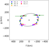 |
Fig. 1 Chords of all the occultations centered in a common reference position, as explained in the text, along with the best fitting ellipse. This ellipse has a semi-major axis (v) of 241.0 ± 7.2 km, a semi-minor axis (u) of 157.1 ± 5.2 km, and an average area-equivalent diameter of 389.2 ± 8.7 km. |
3.2 Geometric albedo
Unfortunately, the rotational period of 2002 KX14 remains unknown. However, through this new average diameter in the visible, along with the most accurate visual magnitude found in the literature (HV = 4.978 ± 0.017; Alvarez-Candal et al. 2016), it is possible to calculate its geometric albedo using Eq. (6) (Russell 1916), where C = 1330 ± 18 km is a constant (Masiero et al. 2021).
 (6)
(6)
This yields a value of pV = 11.9 ± 0.7%.
4 Conclusions and future works
This study presents the analysis of five stellar occultations by the TNO (119951) 2002 KX14 observed between 2020 and 2023. These events yielded 15 positive chords, enabling precise determination of the object’s size, shape, and albedo. Using these occultation data, we derived an average area-equivalent diameter of 389.2 ± 8.7 km, compatible with the  obtained by Alvarez-Candal et al. (2014), and lower than that estimated by Vilenius et al. (2012). The geometric albedo is estimated at 11.9 ± 0.7%, higher than that obtained through thermal observations but within error bars at 3σ.
Objects with a variability lower than 0.15 mag are possibly Maclaurin spheroids (i.e., oblate bodies with two equal axes larger than the third), where this low variability is likely due to the presence of large-scale albedo features on their surface (Thirouin et al. 2010). Thus, given the minimal rotational variability of 2002 KX14, we can reasonably assume that the observed variations are due to albedo features. Since the observed axis ratio (u/v) is 1.53, if we assume a spheroidal shape and adopt a rotation period of 7 hours, which is consistent with the typical values estimated for trans-Neptunian objects (Duffard et al. 2009), we derive a density of approximately 900 kg m−3 using the Chandrasekhar formalism (Chandrasekhar 1987). That said, it is important to note that this density estimate relies on several assumptions that are not directly supported by our dataset, such as a rotation period of 7 hours, although significantly longer periods are equally plausible.
The refined measurements of 2002 KX14’s physical properties demonstrate the effectiveness of stellar occultations in characterizing distant objects in the outer solar system. Currently, the projected shapes of only 13 other TNOs have been determined; among them, 2002 KX14 will be the first cold classical object (although, as explained in Section 1, it is possible that it could belong to the hot population). Either way, regardless of its classification, these results contribute to the growing body of knowledge on the trans-Neptunian region.
In recent years, 2002 KX14 has been passing through the dense star fields of the Milky Way, complicating the acquisition of high-quality light curves needed for determining its rotation period. This difficulty is further compounded by its low rotational amplitude, which remains below 0.05 mag. As the object moves away from this crowded region, opportunities will arise to collect high-precision photometric data. Combining such data with the results presented here will enable the determination of a rotational period and a more comprehensive understanding of 2002 KX14’s physical properties. Additionally, further occultation campaigns may refine the shape and albedo estimated in this work, particularly if more multi-chord events are observed. These efforts could significantly reduce uncertainties in the current models, allowing for the generation of more accurate shape models and potentially determining the object’s spin axis orientation. Future studies will also integrate these results with thermal modeling and spectroscopy to better constrain the object’s surface composition and thermal properties, offering a deeper insight into its evolutionary history.
Acknowledgements
We express our gratitude to observers Marek Harman, Tomas Janik, and Michal Rottenborn for sharing their analysis and contributing it to the Occult software repository. We thank Annie Peck for generously donating observing time for Occ. E analyzed in this study. We thank Riley DeColibus and E. Fernandez for collaborating in the observations. J.L.R., J.L.O., N.M., P.S-S., R.L., M.K., R.M., A.A-C., R.D. and J.M.G-L. acknowledge financial support from the Severo Ochoa grant CEX2021-001131S funded by MCIN/AEI/10.13039/501100011033. J.L.R. acknowledges support from the Ministry of Science and Innovation under the funding of the European Union NextGeneration EU/PRTR. F.L.R. acknowledges CNPq, Brazil grant 103096/2023-0, Florida Space Institute’s Space Research Initiative, 379 and the University of Central Florida’s Preeminent Postdoctoral Program (P3). Part of this work was supported by the Spanish projects PID2020-112789GB-I00 from AEI and Proyecto de Excelencia de la Junta de Andalucía PY20-01309. P.S-S. acknowledges financial support from the Spanish I+D+i project PID2022139555NB-I00 (TNO-JWST) funded by MCIN/AEI/10.13039/501100011033. A.A.-C. acknowledges financial support from the Spanish project PID2023153123NB-I00, funded by MCIN/AEI. G.M.S. thanks the support by the SNN147362 and the GINOP-2.3.2-15-2016-00003 grants of the Hungarian Research, Development and Innovation Office (NKFIH). This work has made use of data from the European Space Agency (ESA) mission Gaia, processed by the Gaia Data Processing and Analysis Consortium (DPAC). Funding for the DPAC has been provided by national institutions, in particular the institutions participating in the Gaia Multilateral Agreement. This work is partly based on observations collected at the Centro Astronómico Hispano en Andalucía (CAHA) at Calar Alto, operated jointly by Junta de Andalucía and Consejo Superior de Investigaciones Científicas (CSIC). This research is also partially based on observations carried out at the Observatorio de Sierra Nevada (OSN) operated by Instituto de Astrofísica de Andalucía (IAA-CSIC). This work is also partly based on observations made with the Tx40 telescope at the Observatorio Astrofísico de Javalambre in Teruel, a Spanish Infraestructura Cientifico-Técnica Singular (ICTS) owned, managed, and operated by the Centro de Estudios de Física del Cosmos de Aragón (CEFCA). Tx40 is funded by the Fondos de Inversiones de Teruel (FITE). This work is also partly based on observations obtained with the Apache Point Observatory 3.5-meter telescope, which is owned and operated by the Astrophysical Research Consortium.
References
- Alvarez-Candal, A., Ortiz, J. L., Morales, N., et al. 2014, A&A, 571, A48 [NASA ADS] [CrossRef] [EDP Sciences] [Google Scholar]
- Alvarez-Candal, A., Pinilla-Alonso, N., Ortiz, J. L., et al. 2016, A&A, 586, A155 [NASA ADS] [CrossRef] [EDP Sciences] [Google Scholar]
- Assafin, M., Santos-Filho, S., Morgado, B. E., et al. 2023, MNRAS, 526, 6193 [Google Scholar]
- Benecchi, S. D., & Sheppard, S. S., 2013, AJ, 145, 124 [Google Scholar]
- Benedetti-Rossi, G., Sicardy, B., Buie, M. W., et al. 2016, AJ, 152, 156 [NASA ADS] [CrossRef] [Google Scholar]
- Benedetti-Rossi, G., Santos-Sanz, P., Ortiz, J. L., et al. 2019, AJ, 158, 159 [NASA ADS] [CrossRef] [Google Scholar]
- Boehnhardt, H., Schulz, D., Protopapa, S., & Götz, C., 2014, Earth Moon Planets, 114, 35 [Google Scholar]
- Chandrasekhar, S., et al. 1987, Ellipsoidal Figures of Equilibrium (New Yprk: Dover Publications) [Google Scholar]
- Collins, K. A., Kielkopf, J. F., Stassun, K. G., & Hessman, F. V., 2017, AJ, 153, 77 [Google Scholar]
- Delsanti, A., & Jewitt, D., 2006, in Solar System Update, eds. Blondel, P., & Mason, J. W. (Berlin, Heidelberg: Springer), 267 [CrossRef] [Google Scholar]
- Desmars, J., Camargo, J. I. B., Braga-Ribas, F., et al. 2015, A&A, 584, A96 [NASA ADS] [CrossRef] [EDP Sciences] [Google Scholar]
- Dias-Oliveira, A., Sicardy, B., Ortiz, J. L., et al. 2017, AJ, 154, 22 [NASA ADS] [CrossRef] [Google Scholar]
- Duffard, R., Ortiz, J. L., Thirouin, A., Santos-Sanz, P., & Morales, N., 2009, A&A, 505, 1283 [NASA ADS] [CrossRef] [EDP Sciences] [Google Scholar]
- Fernández-Valenzuela, E., Pinilla-Alonso, N., Stansberry, J., et al. 2021, Planet. Space J., 2, 10 [Google Scholar]
- Gladman, B., Marsden, B. G., & Vanlaerhoven, C., 2008, in The Solar System Beyond Neptune, eds. Barucci, M. A., Boehnhardt, H., Cruikshank, D. P., Morbidelli, A., & Dotson, R. (Tucson: University of Arizona Press), 43 [Google Scholar]
- Gomes-Júnior, A. R., Morgado, B. E., Benedetti-Rossi, G., et al. 2022, MNRAS, 511, 1167 [CrossRef] [Google Scholar]
- Halíř, R., & Flusser, J., 1998, in International Conference in Central Europe on Computer Graphics and Visualization, https://api.semanticscholar.org/CorpusID:15772208 [Google Scholar]
- Hubbard, W. B., Hunten, D. M., Dieters, S. W., Hill, K. M., & Watson, R. D., 1988, Nature, 336, 452 [NASA ADS] [CrossRef] [Google Scholar]
- Kilic, Y., Braga-Ribas, F., Kaplan, M., et al. 2022, MNRAS, 515, 1346 [NASA ADS] [CrossRef] [Google Scholar]
- Kretlow, M., Ortiz, J. L., Desmars, J., et al. 2024, A&A, 691, A31 [NASA ADS] [CrossRef] [EDP Sciences] [Google Scholar]
- Lasker, B. M., Lattanzi, M. G., McLean, B. J., et al. 2008, AJ, 136, 735 [Google Scholar]
- Masiero, J. R., Wright, E. L., & Mainzer, A. K., 2021, Planet. Sci. J., 2, 32 [Google Scholar]
- Nimmo, F., Umurhan, O., Lisse, C. M., et al. 2017, Icarus, 287, 12 [NASA ADS] [CrossRef] [Google Scholar]
- Ortiz, J. L., Sicardy, B., Braga-Ribas, F., et al. 2012, Nature, 491, 566 [NASA ADS] [CrossRef] [Google Scholar]
- Ortiz, J. L., Santos-Sanz, P., Sicardy, B., et al. 2017, Nature, 550, 219 [NASA ADS] [CrossRef] [Google Scholar]
- Ortiz, J. L., Santos-Sanz, P., Sicardy, B., et al. 2020, A&A, 639, A134 [NASA ADS] [CrossRef] [EDP Sciences] [Google Scholar]
- Peixinho, N., Delsanti, A., Guilbert-Lepoutre, A., Gafeira, R., & Lacerda, P., 2012, A&A, 546, A86 [NASA ADS] [CrossRef] [EDP Sciences] [Google Scholar]
- Pereira, C. L., Sicardy, B., Morgado, B. E., et al. 2023, A&A, 673, L4 [NASA ADS] [CrossRef] [EDP Sciences] [Google Scholar]
- Rommel, F. L., Braga-Ribas, F., Desmars, J., et al. 2020, A&A, 644, A40 [NASA ADS] [CrossRef] [EDP Sciences] [Google Scholar]
- Rommel, F. L., Braga-Ribas, F., Ortiz, J. L., et al. 2023, A&A, 678, A167 [NASA ADS] [CrossRef] [EDP Sciences] [Google Scholar]
- Russell, H. N., et al. 1916, ApJ, 43, 173 [Google Scholar]
- Santos-Sanz, P., Ortiz, J. L., Sicardy, B., et al. 2022, A&A, 664, A130 [NASA ADS] [CrossRef] [EDP Sciences] [Google Scholar]
- Sicardy, B., Ortiz, J. L., Assafin, M., et al. 2011, Nature, 478, 493 [NASA ADS] [CrossRef] [Google Scholar]
- Souami, D., Braga-Ribas, F., Sicardy, B., et al. 2020, A&A, 643, A125 [NASA ADS] [CrossRef] [EDP Sciences] [Google Scholar]
- Stern, S. A., & Trafton, L. M., 2008, in The Solar System Beyond Neptune, eds. Barucci, M. A., Boehnhardt, H., Cruikshank, D. P., Morbidelli, A., & Dotson, R. (Tucson: University of Arizona Press), 365 [Google Scholar]
- Tancredi, G., & Favre, S., 2008, Icarus, 195, 851 [NASA ADS] [CrossRef] [Google Scholar]
- Thirouin, A., Ortiz, J. L., Duffard, R., et al. 2010, A&A, 522, A93 [NASA ADS] [CrossRef] [EDP Sciences] [Google Scholar]
- van Belle, G. T., et al. 1999, PASP, 111, 1515 [NASA ADS] [CrossRef] [Google Scholar]
- Vara-Lubiano, M., Benedetti-Rossi, G., Santos-Sanz, P., et al. 2022, A&A, 663, A121 [NASA ADS] [CrossRef] [EDP Sciences] [Google Scholar]
- Vilenius, E., Kiss, C., Mommert, M., et al. 2012, A&A, 541, A94 [NASA ADS] [CrossRef] [EDP Sciences] [Google Scholar]
- Zacharias, N., Monet, D. G., Levine, S. E., et al. 2004, AAS Meeting Abstracts, 205, 48.15 [Google Scholar]
Appendix A Hertzsprung–Russell diagram of occulted stars and predicted occultation shadow path
Hertzsprung–Russell diagram showing stars from the HYG star database archive5, which combines data from the HIPPARCOS, Yale Bright Star, and Gliese (nearby star) catalogs. The occulted stars analyzed in Section 2 are plotted and are all giant stars. To retrieve the absolute magnitude and temperature of the occulted stars, we used data from the Gaia catalog. The absolute magnitude was calculated using the star’s apparent G magnitude, which was then converted to absolute magnitude via parallax.
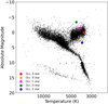 |
Fig. A.1 Absolute magnitude versus temperature of the HYG star database along with the stars occulted by 2002 KX14 and analyzed in this work. |
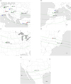 |
Fig. A.2 Predicted occultation shadow path computed from JPL#18 ephemerids for (a) May 26, 2020, (b) June 23, 2022, (c) May 17, 2023, (d) May 19, 2023, and (e) July 01, 2023. The green lines depict the boundaries of the shadow path assuming a 455 km diameter body. The black points indicate the center of the shadow path at 5-second intervals, with the largest point representing the central moment of the prediction. The dots indicate the positions of the stations involved in the campaigns. Green dots signify sites where a positive occultation was observed, red dots a negative occultation, and blue ones indicate low S/N or technical issues (neither positive nor negative). These maps have been generated using SORA. The bottom right arrows denote the shadow’s direction of motion. |
Appendix B Stellar occultation analyses
Light curves from the occultation events described in Section 3. Additionally, tables containing the ingress and egress times after the square well fits are provided, along with the expanded table containing information about the location of telescopes, instruments, and observers.
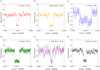 |
Fig. B.1 Normalized flux values obtained from the six positive observations made during Occ. A on May 26, 2020. The solid line represents a square well fit to the observational data. The observing sites and the significance of the drop are indicated in the inserted labels. |
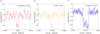 |
Fig. B.2 Normalized flux values obtained from the three positive observations made during Occ. B on June 23, 2022. The solid line represents a square well fit to the observational data. The observing sites and the significance of the drop are indicated in the inserted labels. |
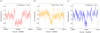 |
Fig. B.3 Normalized flux values obtained from the three positive observations made during Occ. C on May 17, 2023. The solid line represents a square well fit to the observational data. The observing sites and the significance of the drop are indicated in the inserted labels. |
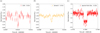 |
Fig. B.4 Normalized flux values from the two positive detections, shown in (a) and (b), during Occ. D on May 19, 2023, while (c) presents the normalized flux from the positive detection during Occ. E on July 1, 2023. In all panels, the solid line represents a square-well fit to the observational data. The observing sites and the significance of the flux drop are indicated in the corresponding labels. |
Observatories, instrumentation, and observers.
UT ingress and egress times and errors for each observation.
Parameters obtained through χ2 minimization for Occ. B, C, D, and E.
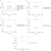 |
Fig. B.5 Chords of the stellar occultations projected on the sky plane. The ingress uncertainties are shown in pink, and the egress uncertainties are in orange. In the legend, the chord length values in kilometers appear alongside the uncertainty error. The ephemeris source used for these plots was JPL#18. |
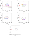 |
Fig. B.6 Chords of the stellar occultations projected on the sky plane along with their fitted ellipses in dashed lines for (a) Occ. A on May 26, 2020, (b) Occ. B on June 23, 2022, (c) Occ. C on May 17, 2023, (d) Occ. D on May 19, 2023, and (e) Occ. E on July 01, 2023. The cross represents the centroid of the ellipse. The ephemeris source used for these plots was JPL#18. |
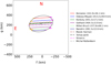 |
Fig. B.7 Six chords and the fitted ellipse for Occ. A on May 26, 2020, shown alongside the three additional chords available in the Occult software. Since the names of the locations are unknown, the legend displays the names of the users who uploaded the data. We also include the Stracise chord, which presents technical issues. The newly incorporated chords are represented as dashed-dotted lines in this figure. We confirm that they remain consistent with the values obtained in this study. |
At the time of writing, more than 5000 objects, including the scattered disk and Centaurs, have been listed at https://minorplanetcenter.net/iau/lists/TNOs.html and https://minorplanetcenter.net/iau/lists/Centaurs.html
Apart from Arrokoth, which was observed up close by the New Horizons mission.
All Tables
All Figures
|
Fig. 1 Chords of all the occultations centered in a common reference position, as explained in the text, along with the best fitting ellipse. This ellipse has a semi-major axis (v) of 241.0 ± 7.2 km, a semi-minor axis (u) of 157.1 ± 5.2 km, and an average area-equivalent diameter of 389.2 ± 8.7 km. |
| In the text | |
|
Fig. A.1 Absolute magnitude versus temperature of the HYG star database along with the stars occulted by 2002 KX14 and analyzed in this work. |
| In the text | |
|
Fig. A.2 Predicted occultation shadow path computed from JPL#18 ephemerids for (a) May 26, 2020, (b) June 23, 2022, (c) May 17, 2023, (d) May 19, 2023, and (e) July 01, 2023. The green lines depict the boundaries of the shadow path assuming a 455 km diameter body. The black points indicate the center of the shadow path at 5-second intervals, with the largest point representing the central moment of the prediction. The dots indicate the positions of the stations involved in the campaigns. Green dots signify sites where a positive occultation was observed, red dots a negative occultation, and blue ones indicate low S/N or technical issues (neither positive nor negative). These maps have been generated using SORA. The bottom right arrows denote the shadow’s direction of motion. |
| In the text | |
|
Fig. B.1 Normalized flux values obtained from the six positive observations made during Occ. A on May 26, 2020. The solid line represents a square well fit to the observational data. The observing sites and the significance of the drop are indicated in the inserted labels. |
| In the text | |
|
Fig. B.2 Normalized flux values obtained from the three positive observations made during Occ. B on June 23, 2022. The solid line represents a square well fit to the observational data. The observing sites and the significance of the drop are indicated in the inserted labels. |
| In the text | |
|
Fig. B.3 Normalized flux values obtained from the three positive observations made during Occ. C on May 17, 2023. The solid line represents a square well fit to the observational data. The observing sites and the significance of the drop are indicated in the inserted labels. |
| In the text | |
|
Fig. B.4 Normalized flux values from the two positive detections, shown in (a) and (b), during Occ. D on May 19, 2023, while (c) presents the normalized flux from the positive detection during Occ. E on July 1, 2023. In all panels, the solid line represents a square-well fit to the observational data. The observing sites and the significance of the flux drop are indicated in the corresponding labels. |
| In the text | |
|
Fig. B.5 Chords of the stellar occultations projected on the sky plane. The ingress uncertainties are shown in pink, and the egress uncertainties are in orange. In the legend, the chord length values in kilometers appear alongside the uncertainty error. The ephemeris source used for these plots was JPL#18. |
| In the text | |
|
Fig. B.6 Chords of the stellar occultations projected on the sky plane along with their fitted ellipses in dashed lines for (a) Occ. A on May 26, 2020, (b) Occ. B on June 23, 2022, (c) Occ. C on May 17, 2023, (d) Occ. D on May 19, 2023, and (e) Occ. E on July 01, 2023. The cross represents the centroid of the ellipse. The ephemeris source used for these plots was JPL#18. |
| In the text | |
|
Fig. B.7 Six chords and the fitted ellipse for Occ. A on May 26, 2020, shown alongside the three additional chords available in the Occult software. Since the names of the locations are unknown, the legend displays the names of the users who uploaded the data. We also include the Stracise chord, which presents technical issues. The newly incorporated chords are represented as dashed-dotted lines in this figure. We confirm that they remain consistent with the values obtained in this study. |
| In the text | |
Current usage metrics show cumulative count of Article Views (full-text article views including HTML views, PDF and ePub downloads, according to the available data) and Abstracts Views on Vision4Press platform.
Data correspond to usage on the plateform after 2015. The current usage metrics is available 48-96 hours after online publication and is updated daily on week days.
Initial download of the metrics may take a while.