| Issue |
A&A
Volume 689, September 2024
|
|
|---|---|---|
| Article Number | A319 | |
| Number of page(s) | 16 | |
| Section | Astrophysical processes | |
| DOI | https://doi.org/10.1051/0004-6361/202450091 | |
| Published online | 23 September 2024 | |
CO2 and NO2 formation on amorphous solid water
Department of Chemistry, University of Basel, Klingelbergstrasse 80, CH-4056 Basel, Switzerland
Received:
22
March
2024
Accepted:
8
June
2024
Abstract
Context. The dynamics of molecule formation, relaxation, diffusion, and desorption on amorphous solid water (ASW) is studied in a quantitative fashion.
Aims. The formation probability, stabilization, energy relaxation, and diffusion dynamics of CO2 and NO2 on cold ASW following atom+diatom recombination reactions are characterized quantitatively.
Methods. Accurate machine-learned energy functions combined with fluctuating charge models were used to investigate the diffusion, interactions, and recombination dynamics of atomic oxygen with CO and NO on ASW. Energy relaxation to the ASW and into water internal degrees of freedom were determined from the analysis of the vibrational density of states. The surface diffusion and desorption energetics were investigated with extended and nonequilibrium MD simulations.
Results. The reaction probability is determined quantitatively and it is demonstrated that surface diffusion of the reactants on the nanosecond time scale leads to recombination for initial separations of up to 20 Å. After recombination, both CO2 and NO2 stabilize by energy transfer to water internal and surface phonon modes on the picosecond timescale. The average diffusion barriers and desorption energies agree with those reported from experiments, which validates the energy functions. After recombination, the triatomic products diffuse easily, which contrasts with the equilibrium situation, in which both CO2 and NO2 are stationary on the multinanosecond timescale.
Key words: astrochemistry / atomic processes / diffusion / molecular processes / ISM: atoms / ISM: molecules
Publisher note: The acknowledgements were corrected on 18 October 2024.
Corresponding author; This email address is being protected from spambots. You need JavaScript enabled to view it. .
© The Authors 2024
 Open Access article, published by EDP Sciences, under the terms of the Creative Commons Attribution License (https://creativecommons.org/licenses/by/4.0), which permits unrestricted use, distribution, and reproduction in any medium, provided the original work is properly cited.
This article is published in open access under the Subscribe to Open model. This email address is being protected from spambots. You need JavaScript enabled to view it. to support open access publication.
1. Introduction
Surface processes are of paramount importance for the genesis of molecules in the Universe. In the interstellar medium, nitrogen emerges as one of the chemically dynamic species, following hydrogen, oxygen, and carbon. Within the realm of prebiotic molecules and simple amino acids, including CH2NH, CH3NH2, NH2CH2COOH, NH2CHO, and HNCO, nitrogen stands out as the common element, underscoring the necessity to explore the reactivity of nitrogen-containing molecules. This is because three-body collisions in the gas phase are highly inefficient for molecule formation from atomic constituents. Astrophysically relevant surfaces consist of silicates, carbonaceous species (graphite, amorphous carbon, polyaromatic hydrocarbons), or water (Herbst 2001). In cold molecular clouds, cosmic dust grains are typically covered by water ice, which can be polycrystalline or amorphous which is also referred to as amorphous solid water (ASW). At low temperatures, ASW dominates over the polycrystalline phase (Wakelam et al. 2017a). Typically, bulk water is present in the form of ASW, which is the main component of interstellar ices (Hagen & Tielens 1981). The structure of ASW is usually probed by spectroscopic measurements (Hagen & Tielens 1981; Jenniskens & Blake 1994), although interference-based methods have also been employed (Bossa et al. 2012). ASWs are porous structures characterized by surface roughness and internal cavities of different sizes, which can retain molecular or atomic guests (Bar-Nun et al. 1987). Under laboratory conditions, water ices have been found to be porous (He et al. 2016; Kouchi et al. 2020) or nonporous (Oba et al. 2009; He et al. 2016; Kouchi et al. 2020), whereas the morphology of ices in the interstellar medium is more heavily debated (Keane et al. 2001; Kouchi et al. 2021).
The high porosity of ASW (Bossa et al. 2014, 2015; Cazaux et al. 2015) makes it a suitable catalyst for gas–surface reactions involving oxygen (Ioppolo et al. 2011; Romanzin et al. 2011; Chaabouni et al. 2012; Minissale et al. 2013a; Dulieu et al. 2017; Pezzella et al. 2018; Pezzella & Meuwly 2019; Christianson & Garrod 2021), hydrogen (Hama & Watanabe 2013), carbonaceous (Minissale et al. 2013b, 2016b; Qasim et al. 2020; Molpeceres et al. 2021), and nitrogen-containing (Minissale et al. 2014) species. The surface morphology and chemistry help to adsorb chemical reagents on top of (Minissale et al. 2019) or inside ASW (Minissale et al. 2016a; Tsuge et al. 2020). This increases the probability that the reaction partners will diffuse to locations for collisions and association reactions to occur. As the diffusivity of individual atoms and small molecules has been established from both experiments and simulations (Minissale et al. 2013b; Lee & Meuwly 2014; Pezzella et al. 2018), this is a likely scenario for the formation of molecules on and within ASW.
The chemical precursors for the formation of CO2 are believed to be carbon monoxide and atomic oxygen. In the past, the CO+O reaction was proposed as a nonenergetic pathway for CO2 formation based on experiments involving a copper surface covered by a water-ice cap with CO and O deposited on it (Roser et al. 2001). The formation of CO2( ) from ground-state CO(1Σ+) and electronically excited O(1D) is barrierless (Talbi et al. 2006; Veliz et al. 2021). In addition to CO2, nitrogen-containing species, such as nitric oxide (NO) (Liszt & Turner 1978; Ligterink et al. 2018; Codella et al. 2018; Ziurys et al. 1991; McGonagle et al. 1990), nitrous oxide (N2O) (Ziurys et al. 1994; Ligterink et al. 2018), and nitrosyl hydride (HNO) (Snyder et al. 1993) have been detected in the interstellar medium. However, their interstellar chemistry has been little explored so far. Specifically, NO is believed to be critical for the overall nitrogen chemistry of the interstellar medium (de Barros et al. 2016; Congiu et al. 2012).
The aim of the present work is to investigate the energetics and dynamics of the CO and NO oxygenation reactions O(1D)+CO(1Σ+) (Veliz et al. 2021) and O(3P)+NO(X2Π) (Veliz et al. 2020; Ndengué et al. 2021) on ASW to form ground-state CO2( ) and NO2(2A′), respectively, at conditions representative of interstellar environments. Electronically excited atomic oxygen species generated from photolysis of H2O has a radiative lifetime of 110 minutes (Garstang 1951). An alternative pathway proceeds via electron-induced neutral dissociation of water into H2 + O(1D) (Schmidt et al. 2019). In the presence of CO, the formation of CO2 in cryogenic CO/H2O films was observed (Schmidt et al. 2019). Ground state 3P atomic oxygen was observed from photolysis of O2 using far-ultraviolet light (Chou et al. 2018). These are also formation routes of O(3P/1D) that can occur in interstellar, photon-dominated regions.
At the low temperatures prevalent in the interstellar medium, surface diffusion of reaction partners is a major driving force for chemical reactions. Earlier work on the CO + O → CO2 recombination reaction (Upadhyay et al. 2021) assumed that the CO and O moieties retain their total charges upon dissociation of OCO → O + CO. This, however, is unrealistic as a CO molecule and an oxygen atom are electrically neutral for large separations between them. To provide a physically meaningful description, a fluctuating point charge (FPC) model is developed in the present work. Such a model describes each of the reactant species as a neutral atom (oxygen) or molecule (CO or NO), respectively, while leading to physically meaningful charges for the reaction products (CO2 and NO2).
The methods used are described below, before presenting the CO2 and NO2 formation dynamics in their electronic ground states. Subsequently, the desorption dynamics of the species involved is described and the energy redistribution is analyzed. Conclusions are drawn in the final section of this work.
2. Methods
2.1. Intermolecular interactions
Reactive molecular dynamics (MD) simulations require potential energy surfaces (PESs) that allow bond formation and bond breaking. Two such PESs were considered in the present work for the [COO] and [NOO] reactive collision systems. First, for both systems, global and reactive PESs are available, which are based on reproducing kernel Hilbert space (RKHS) (Unke & Meuwly 2017) representations (Veliz et al. 2020, 2021). For the [COO] system, the PES was based on extensive CCSD(T)-F12/aug-cc-pVTZ-F12 reference data (Upadhyay et al. 2021), whereas for [NOO] the MRCI+Q/aug-cc-pVTZ level of theory was used (Veliz et al. 2020). For both systems, all asymptotic channels are correctly described, including the atomization reaction. Second, a simplified parametrization was used that is based on Morse oscillators for the bond-stretch degrees of freedom and a harmonic potential for the bending vibration. This Morse–Morse–harmonic model is referred to as MMH. Such a simplified model is considered because of its much improved computational efficiency and because it offers the opportunity to explore the use of such simplified models for investigating larger molecules, for which high-level electronic structure calculations are problematic or unfeasible. It is stressed that both representations, RKHS and MMH, are capable of describing bond formation and bond breaking; that is, these are reactive energy functions for the [COO] and [NOO] systems (Veliz et al. 2020, 2021).
The use of RKHS representations has been validated in gas-phase experiments and they showed excellent performance (Veliz et al. 2020, 2021; Upadhyay et al. 2021). For the MMH parametrizations, Morse potentials V(r) = De(1 − exp( − β(r − r0)))2 were fit to reference calculations at the MRCI/aug-cc-pVTZ level of theory, which was carried out using the MOLPRO (Werner et al. 2020) suite of programs (Werner et al. 2020). To this end, the OB–COA separation (see Figure A.1 for labeling) was scanned on a regular grid of R− values between 0.9 and 6.0 Å, where R is the separation between OB and the center of mass of COA. The same procedure was followed for OB–NOA; see Figure A.1. For the bending degree of freedom, the equilibrium angles were 180° and 134.2° for CO2 and NO2, respectively, and the force constants were 45.0 and 93.0 kcal/mol/radian2. This yields normal mode bending frequencies of 660 cm−1 and 750 cm−1 , compared with 667 cm−1 and 750 cm−1 from experiments (Shimanouchi et al. 1978; Arakawa & Nielsen 1958). Such an approach is similar to that previously taken to explore oxygen–oxygen recombination on amorphous solid water (Pezzella & Meuwly 2019; Pezzella et al. 2020).
The fluctuating point charge model provides a means to correctly describe the asymptotic charge distributions in the reactant and product channels and to smoothly connect the two. Starting from separated neutral reactant species (CO+O and NO+O), upon recombination the charges on all atoms change as a function of the OB–COA and OB–NOA separations; see Figure A.1. In addition, to account for the influence of the surface water molecules on the charges of the adsorbates (O atom, CO, NO, CO2, and NO2), electronic structure calculations for all species including the ten nearest water molecules –corresponding to a first hydration layer– were carried out. This was done at the M062x/aug-cc-pVTZ level of theory using the Gaussian program from which Mulliken charges were extracted (Frisch et al. 2016); charges based on a natural bond orbital (NBO) analysis (Glendening et al. 2012) are discussed in the Section 3. After inspection of the charge variations depending on geometry, a sigmoidal function 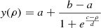 was used to represent charges depending on the separation ρ between the oxygen atom OB and the carbon atom of COA or the nitrogen atom of NOA, respectively; see Figure A.1. As can be seen in Figures A.1A and B, the total charge of CO2 and NO2 is approximately zero, which is consistent with earlier work (Talbi et al. 2006). In other words, there is almost no charge transfer between the adsorbates and ASW.
2.2. Molecular dynamics simulations
All MD simulations were carried out using the CHARMM suite of programs (Brooks et al. 2009) with provisions for bond forming reactions through MMH or RKHS representations (Unke & Meuwly 2017). The simulation system (see Figure 1) consists of an equilibrated cubic box of ASW containing 1000 water molecules with dimensions of 31 × 31 × 31 Å3. Simulations were started from an existing, equilibrated, and validated ASW structure with a realistic distribution of internal cavity volumes (Lee & Meuwly 2014; Pezzella et al. 2018; Pezzella & Meuwly 2019; Upadhyay et al. 2021). For water, the TIP3P model (Jorgensen et al. 1983), as implemented in the CGenFF force field (Vanommeslaeghe & MacKerell 2012), was used for consistency with the van der Waals parameters [ϵ, σ] for C: [–0.11 kcal/mol, 2.1 Å]; O: [–0.12 kcal/mol, 1.7Å]; N: [–0.2 kcal/mol, 1.85 Å], respectively.
 |
Fig. 1. Simulation system for studying CO2 (panel A) and NO2 (panel B) recombination. Panel A color code: Oxygen (red), CO (cyan), CO2 (orange). Panel B color code: Oxygen (red), NO (blue), NO2 (yellow). Before and after recombination, all species diffuse on the ASW. |
Simulations for the formation of triatomics (CO2 and NO2) used a two-dimensional grid (R, θ) with R ∈ [2.0 − 16] Å and θ ∈ [50 − 180]°. For each combination of (R, θ), the reactants ([OB, COA], and [OB, NOA]) were placed randomly on the ASW to broadly sample the surface. First, the structure of the system was optimized (750 steps of steepest descent and 100 steps of adopted basis Newton-Raphson minimization), with R and θ constrained (frozen) to each of the values on the grid. Next, Boltzmann-distributed velocities at 50 K were assigned to all atoms, followed by 50 ps of heating simulations (NVT) to 50 K and 100 ps of equilibration at 50 K, with (R, θ) still constrained. After releasing the constraints, a 500 ps equilibrium trajectory followed, during which coordinates and velocities were saved regularly to obtain 1000 initial conditions for R > 4 Å and 500 for R < 4 Å, accounting for the fact that the reaction probability is ∼1 for short initial R. This yielded a statistically significant number of initial conditions from which CO2 and NO2 recombination trajectories were run. The subsequent production simulations were each 500 ps in length and were carried out in the NVE ensemble to ensure total energy conservation and to be able to analyze energy flow. For analysis, the total energies, coordinates, and velocities were saved every 0.5 ps.
2.3. Analysis
To characterize energy flow between the activated internal modes of newly formed species and the surface water molecules, the vibrational density of states (vDOS) was analyzed (Gaigeot et al. 2007; Ferrero et al. 2023). For this, the Fourier transform of the hydrogen atoms normalized velocity autocorrelation function was determined (Futrelle & McGinty 1971) according to
 (1)
(1)
where v denotes the velocity vector of the hydrogen atom. The value Tc = 1 ps was chosen because vibrational energy flow is expected to occur on such timescales (Mizutani & Mizuno 2022) and because sufficient data for meaningful analysis can be accumulated from the simulations while still covering the tens-of-picoseconds timescale on which the equilibration of the newly formed triatomic molecules takes place. The formation probability of products was determined from the ratio of the number of successful recombination reactions to the total number of reactive collisions, as is usual from rate calculations in quasiclassical trajectory simulations (Truhlar & Muckerman 1979).
3. Results
3.1. Exploratory simulations
A representative 500 ps trajectory for COA + OB recombination is shown in Figure 2 (left column), where OA and OB label the two oxygen atoms to distinguish them; see Figure A.1 for labeling. Initially, the C⋯OB separation was ∼12 Å (see panel A), which is in the asymptotic, noninteracting regime of the COA–OB PES. For the first 190 ps, oxygen diffusion on the water surface can be seen. Upon recombination at t ∼ 190 ps, the CO stretch and the OCO (panel B) angle are highly excited and relax during the following few picoseconds to average values of around the CO2 equilibrium geometry. The CO2 product remains in an internally excited state for a considerably longer timescale; see panel B. The temperatures of the ASW (cyan) and the full system (black) are determined by the kinetic energies of the molecules. A prominent peak in the temperature of the full system is observed immediately after recombination, whereas the warming of cool water surface is gradual (panel C inset).
 |
Fig. 2. Recombination of CO + O to form CO2 (left column) and NO + O to NO2 (right column) in ground state. Panels A and D: OB–C/N (red) and OA–C/N (black) separation. Panels B and E: O–C/N–O angle. Panels C and F: Temperature of the ASW (cyan) and the full system (black) before and after recombination. Upon recombination, both O–C/N stretches exhibit equally pronounced excitation (shown in the insets). |
Figure 2 (right column) shows a NOA + OB recombination trajectory. The ground state NO2(2A′) has a nonlinear geometry with N-O distances of 1.2 Å and an O-N-O angle of 134°. In this case, recombination takes place after ∼110 ps and the amount of energy released is half compared to the CO2. This is due to the different stabilization energies of the triatomics with respect to the CO/NO+O asymptote, which are 7.71 eV for CO2 (for θ = 180°) and 3.24 eV for NO2 (for θ = 135°), respectively.
3.2. Reaction probabilities for CO2 and NO2 formation
The formation dynamics of CO2 and NO2 was followed from initial conditions on a (R, θ) grid. For each initial R and θ configuration, 250 or 500 trajectories at 50 K were run for 500 ps. Depending on the initial (R, θ) values, heat maps of the formation probability were determined and a kernel density estimate (KDE) was used for smoothing; see Figures 3 and 4.
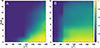 |
Fig. 3. KDE density map for the average CO2 formation probability depending on initial (R, θ) using the MMH (Panel A) and RKHS (Panel B) PES. The color palette indicates the probability of the reaction, with yellow representing P = 1 and blue representing P = 0. The COO formation probability using RKHS PES is shown in Figure A.2. |
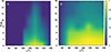 |
Fig. 4. NO2 formation probability as a function of R and θ using MMH (Panel A) and RKHS (Panel B) PES. The color palette indicates the probability of the reaction, with yellow representing P = 1 and blue representing P = 0. |
Figure 3 reports probability heat maps for the likelihood to form CO2 depending on initial (R, θ) using both MMH (Panel A) and RKHS (Panel B) PESs from simulations of 500 ps in length. With the MMH PES (Panel A) for R ∼ 2 to 4.5 Å, the recombination probability is P ∼ 1 near 180° and vanishes for θ ∼ 90°. For θ = 180°, P changes from unity for R = 4 to P ∼ 0 for 14 Å on the 500 ps timescale. For R > 4 Å and θ ≤ 120°, the formation probability is P = 0.
Using the RKHS PES, which is a considerably more accurate representation of the O+CO interaction than the MMH parametrization, the reaction probabilities depending on initial (R, θ) are larger throughout; see Figure 3 B. The probability for formation of CO2 is particularly increased along the angular coordinate θ. These differences are due to the different topographies of the two PESs. Also, the angular dependence is observed for R < 7Å, and for larger distances, R > 7Å, a plateau is observed. This plateau implies that the reaction probability is primarily governed by diffusion for large distances and does not depend on the initial angular term on the 500 ps timescale.
Due to the more realistic and improved charge model for the reactants, their diffusivity increases. For simulations on the 500 ps, this leads to a nonvanishing reaction probability for initial separations of R = 16 Å. This contrasts remarkably with earlier simulations (Upadhyay et al. 2021) that maintained the charges on the oxygen atom and CO molecule fixed at ±0.3e (corresponding to their charges in CO2), which suppressed the reactants’ mobility and reaction probability for R > 5 Å for simulations on the same timescale. Overall, using the more realistic charge models from the present work increases the recombination probability of the species involved.
The recombination probability for NO2 formation is reported in Figure 4. Panel A shows the 2D recombination probability using the MMH PES. For NO2, the minimum energy structure has θ = 134°, which leads to P ∼ 1 for θ ∈ [125, 145]° and R ≤ 4 Å, which gradually decreases to P ∼ 0 as R increases. Using the considerably more accurate RKHS representation, the recombination probability is larger throughout; see Figure 4B. A formation probability of P ∼ 1 is found for θ ∈ [90, 180]° and R ≤ 8 Å. These differences are again due to the different topographies of the two PESs. Similar to CO2, the recombination probability is not equal to zero at R = 16 Å on the 500 ps timescale and a plateau is observed for R > 8Å.
Although the structures of CO2 and NO2 differ (linear versus bent), the shape of the underlying PES is reflected for both in the geometry dependence of the rebinding probability for shorter R. For larger initial separations R, the rebinding probability is purely governed by diffusion and is independent of θ. Taking the results from simulations using the RKHS representation as the reference, the MMH PES yields qualitatively comparable results. However, in particular for NO2 the reaction funnel is far too narrow. On the other hand, the MMH-PES is orders of magnitude more computationally efficient and improvements with techniques such as multistate adiabatic reactive MD (MS-ARMD) may yield considerable improvements over MMH (Nagy et al. 2014; Upadhyay & Meuwly 2021).
The RKHS PES also supports the COO conformation and results in the formation and stabilization of COO. This intermediate holds significant interest as it can decay to C + O2. The probability heat map for the likelihood to form COO depending on R and θ is shown in Figure A.2. Finally, the atom exchange reaction is found for 7 % of all simulations using the MMH PES for NO/CO + O. Atom exchange with RKHS is not observed for CO+O, whereas 0.4 % of the simulations show atom exchange for NO + O collision.
3.3. Energy dissipation upon triatomic product relaxation
Both association reactions considered here are exothermic. Upon recombination, products are formed in a highly excited internal state (vibration and rotation) and their relaxation depends on the coupling between excited stretching and bending modes of the newly formed species and phonon and internal modes of the underlying water ice surface (Ferrero et al. 2023). To allow energy transfer between the adsorbate and the internal and phonon modes of ASW, the reparametrized (Burnham et al. 1997; Plattner & Meuwly 2008) flexible Kumagai, Kawamura, and Yokokawa (KKY) water model (Kumagai et al. 1994) was used in these simulations. This model has been successfully used to study the spectroscopy of CO on and in ices (Plattner & Meuwly 2008), the vibrational relaxation of solvated cyanide (Lee & Meuwly 2011), and the relaxation of O2 formed on ASW following O(3P)+O(3P) recombination and vibrational relaxation through coupling to the water-phonon modes (Pezzella & Meuwly 2019). Within 1 μs, O2 relaxes to the v = 2 vibrational state, which is consistent with experimental findings (Hama et al. 2010) and validates the use of the KKY model to study energy transfer processes involving ASW.
To study energy dissipation following recombination, several hundred O+CO→CO2 and O+NO→NO2 trajectories were run for 500 ps. Subsequently, 280 recombination trajectories were analyzed for CO2 and NO2, respectively. First, the normalized final kinetic energy distribution  at 450 ps after recombination was determined for the products; see Figure A.3. The
  for CO2 and NO2 extend from low-
 (∼1 kcal/mol) to 60 kcal/mol. For NO2, more than 80 % of the products contain
  kcal/mol after 450 ps, whereas for CO2 this fraction is considerably smaller. In other words, relaxation of the highly excited internal modes is more effective for NO2 compared with CO2. Possible reasons for such rapid relaxation include but are not limited to the shallow minimum for NO2 compared to CO2 and/or more efficient coupling of the vibrational modes of NO2 to the surrounding water molecules.
Next, for one CO2-forming trajectory, the kinetic energy distribution and vDOS of two water molecules WA and WB and the CO2 molecule were determined for windows of 1 ps in length; see Figure 5. For the analysis, the time of recombination was set to zero and water molecules WA and WB were chosen such that, at t = 0, WA was the water molecule nearest to the newly formed CO2 and WB was closest to CO2 after 3.0 ps due to diffusion of the recombination product. As a reference point for the analysis, the averaged Ekin (red distributions) and vDOS (black lines) for ten water molecules away from the recombination site was determined for the 0.5 ps prior to CO2-formation; see the top row in Figure 5.
 |
Fig. 5. Vibrational density of states power spectrum (in black) and P(Ekin) (red) for water molecules A and B, WA (panel A) and WB (panel B), on the ASW surface at several delay times after the formation of CO2 on the RKHS-PES. The IR bands at 1600 − 1750 and 3200 − 3600 cm−1 correspond to bending and OH-stretching modes (Hagen & Tielens 1981; Yu et al. 2020; Devlin 1990). Panel C reports the kinetic energy distribution (red) and the vDOS of the CO2 molecule. Top panel: Averaged vDOS spectrum and kinetic energy distribution for ten water molecules away from the recombination site determined for the 0.5 ps prior to CO2 formation. Subsequent panels are labeled with the time interval after CO2 recombination. See Figure A.4 for an analysis of a trajectory using the MMH PES. |
For water molecule WA, the maximum of P(Ekin) (red shaded area) shifts to higher Ekin and its width increases considerably for the first 15 ps after recombination. Energy flow is clearly taking place as can be seen from the varying widths and locations of the maxima depending on time after recombination. The same is observed for water molecule WB (middle column). As judged from the vDOS (black lines), the water stretch, bend, and libration modes for WA and WB are populated for all time intervals. The two internal modes do not shift in frequency relative to the thermal equilibrium and their frequency is covered by the experimentally determined frequency range (Hagen & Tielens 1981; Yu et al. 2020; Devlin 1990).
The CO2 molecule formed is initially highly excited, which leads to a broad, unstructured P(Ekin); see the top panel in Figure 5C. Over the next 15 ps, the width of P(Ekin) rapidly decreases due to energy exchange with the internal modes of the surrounding water molecules and the phonon modes of the ASW. The reaction product does not further cool until 60 ps after recombination. A picture emerges for the vDOS that is rather different than that for water. The vibrational frequencies for CO2 are at 667 (bend), 1333 (symmetric stretch), and 2349 (antisymmetric stretch) cm−1 from experiments (Shimanouchi et al. 1978) (see vertical lines) and 647, 1374, and 2353 cm−1 from calculations using the reactive PES, in reasonably good agreement. For times up to 5 ps after recombination, only frequencies below ∼1000 cm−1 appear in the vDOS. Specifically, the antisymmetric stretch mode only manifests itself after ∼6 ps, because the reactive PES for CO2 is fully anharmonic and for the first few picoseconds after recombination the highly excited stretching motions sample the narrowly spaced energies close to dissociation. For times between 6 ps and 14 ps after recombination, the asymmetric stretch shifts from ∼1800 cm−1 to 2250 cm−1 due to relaxation from higher to lower vibrationally excited states. The CO2 bending vibration together with its overtone at 1130 cm−1 are prominently populated after 4 ps until 12 ps, after which the symmetric stretch appears and the overtone disappears.
A slightly different approach was used for NO2 recombination in order to study the energy transfer between neighboring water molecules on the ASW. Again, P(Ekin) and the vDOS of water molecules WA and WB and NO2 were determined for one NO2−forming trajectory. In this case, WA is the water molecule closest to NO2, while WB is hydrogen-bonded to WA; see Figure 6. For the first 1 ps after recombination, the widths of P(Ekin) for WA and WB are considerably broader than the thermal distribution; see the top panel of Figure 6A. Energy exchange between the two water molecules is readily observed for the following 5 ps with maxima and widths of P(Ekin) increasing and decreasing. The distributions for 10 ps and 40 ps no longer change appreciably and the two water molecules do not fully thermalize on that timescale. The kinetic energy distribution for NO2 is broad at the beginning (50 kcal/mol) and transfers more than half of this energy to the environment within 10 ps of recombination (Figure 6C).
 |
Fig. 6. Vibrational density of states power spectrum (in black) and P(Ekin) (red) for water molecules A and B, WA (panel A) and WB (panel B), on the ASW surface at several delay times after the formation of NO2 on the RKHS-PES. The IR bands at 1600 − 1750 and 3200 − 3600 cm−1 correspond to bending and OH-stretching modes (Hagen & Tielens 1981; Yu et al. 2020; Devlin 1990). Panel C reports the kinetic energy distribution (red) and the vDOS of the NO2 molecule. For an analysis of a trajectory using the MMH PES, see Figure A.5. |
The experimentally measured (Arakawa & Nielsen 1958) vibrational frequencies for gas phase NO2 are at 750 (bend), 1318 (symmetric stretch), and 1618 (antisymmetric stretch) cm−1. Up to 4 ps after recombination, the vDOS is rather sparse. Regarding CO2, the asymmetric stretch mode is not populated at all at early times, whereas the bend and symmetric stretch manifest themselves by 6 ps. At 10 and 40 ps after recombination, the NO2 vibrational spectrum can be recognized from the vDOS. For the water modes, the librational and stretching modes are populated throughout, whereas the bending mode is present occasionally and clearly visible after 40 ps.
Specifically comparing the time evolution of P(Ekin) for CO2 and NO2, the two products are found to differ in the efficiency and speed of cooling. For NO2, the fraction of products formed with Ekin ∼ 5 kcal/mol within 450 ps is twice as large as it is for CO2; see Figure A.3. This may be related to the lower energy of formation (3.24 eV vs. 7.71 eV) but may also be due to the overall lower vibrational energies of the fundamentals for NO2 compared with CO2, which facilitates energy relaxation.
For a mode-specific analysis of energy transfer between the formed CO2 and the surrounding water molecules, the time evolution of the integrated vDOS in three frequency ranges was considered: water libration: (0 − 1000 cm−1), bending (1500 − 2000 cm−1), and stretching (2800 − 3800 cm−1). For this analysis, water molecules within 10 Å in the x−direction and 5 Å in the y/z− direction around the recombination site were used; see Figure A.6. The vDOS was then computed for each water molecule separately, and the resulting peak areas were averaged over 100 water molecules located in the region defined above. Figure 7A reports the difference between the equilibrium averaged peak area and the area at time t after recombination. Alternatively, the difference between peak area immediately after excitation and the area at time t is shown in panel B. The integrated intensity of the low-frequency libration mode (black line) initially increases, followed by a decrease after ∼10 ps, before eventually reaching a plateau after 25 ps (panel A). Meanwhile, the intensity of the stretching modes (green) displays a progressive rise over the first 25 ps, followed by fluctuations around a specific value, and then a slow relaxation over about 100 ps. In comparison, the intensity of bending modes (red traces) remains comparable throughout the observed time frame (a similar observation is shown in Figure A.7). The time series show that the libration mode first acquires and stores energy and subsequently releases it, whereas the stretching modes pick up energy over a timscale of approximately 100 ps and retain it beyond that. This was also observed for NH3 formation on water ice (Ferrero et al. 2023).
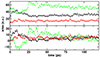 |
Fig. 7. Time evolution of the integrated change of vDOS curves averaged over 100 water molecules for libration (black), bending (red), and stretching modes (green) of water using the RKHS-PES. In panel A, the equilibrium, thermally averaged area before recombination is the reference for calculating the difference at time t, whereas for panel B, the peak area immediately after excitation (t = 1ps) is the reference. Here, solid lines represent the four-point moving average. For an analysis using the MMH PES, see Figure A.8. |
3.4. Species desorption on ASW
To explicitly probe desorption, velocities for the adsorbants (CO, NO, CO2, and NO2) were drawn from a Maxwell-Boltzmann distribution and scaled along the x-direction, perpendicular to the water surface (Pezzella et al. 2020). For the water molecules, the velocities were those from an equilibrium simulation at 50 K and the dynamics of the system was followed for 100 ps. If within this timescale the adsorbant remained on the ASW, it was considered physisorbed. However, for sufficiently large scaling of the velocity vector, the adsorbant leaves the ASW from which the desorption energy can be estimated (Pezzella et al. 2020). Average desorption energies were determined for initiating the dynamics for different initial positions of the adsorbant on the ASW.
Computed desorption energies (Edes) for CO and NO from the ASW surface were 3.5 ± 0.7 kcal/mol (1812 K or 156 meV) and 3.1 ± 0.5 kcal/mol (1534 K or 132 meV), respectively. Earlier MD simulations reported (Upadhyay et al. 2021) CO-desorption energies of between 3.1 and 4.0 kcal/mol (1560 K to 2012 K or 130 meV to 170 meV), compared with 120 meV (2.8 kcal/mol or 1392 K) from experiments (Karssemeijer et al. 2013). It was also found that the desorption energy of CO from ASW depends on CO coverage with ranges from Edes = 1700 K for low to Edes = 1000 K for high coverage, respectively (He et al. 2016), which supports the simulation results (Upadhyay et al. 2021). On nonporous and crystalline water surfaces, submonolayer desorption energies for CO are 1307 K and 1330 K (∼115 meV), respectively (Noble et al. 2012). For NO, experiments reveal a desorption energy of 1300 K (2.6 kcal/mol or 112 meV) when using temperature programmed desorption measurements (Minissale et al. 2019) after exposure of NO/H2O ice to atomic oxygen. Thus, for both diatomics, the present findings are consistent with experiments and earlier simulations.
For the triatomics, computed average desorption energies for CO2 and NO2 from ASW were 9.0 ± 1.9 kcal/mol (4529 K or 390 meV) and 13.1 ± 3.4 kcal/mol (6592 K and 568 meV). For CO2, one experiment reported Edes = 2490 ± 240 K (Galvez et al. 2007) (4.9 ± 0.47 kcal/mol or 214 ± 20 meV) whereas a compilation of literature data reported desorption energies ranging from 4.5 to 6.0 kcal/mol (Wakelam et al. 2017b), all of which are considerably lower than the computed values. This indicates that the electrostatic interaction between CO2 and the surface is somewhat too strong. Yet, recomputing CO2 point charges using an alternative and potentially more physical NBO (Glendening et al. 2012) analysis yields increased polarity and interaction strengths with ASW for CO2 (see Figure A.9), which is inconsistent with experimental findings. On the other hand, no experimentally measured data are available for NO2 (Wakelam et al. 2017b); however, the desorption temperatures of NO2 and H2O from the same ice surface were found to be comparable, which indicates that NO2 interacts strongly with the surface (Ioppolo et al. 2014). Overall, for all four species relevant to the present work, the computed Edes compare reasonably (CO2) to favorably (CO, NO) with reference values from experiments and previous calculations, particularly in light of the fact that appreciable variations in experimentally reported values exist (Wakelam et al. 2017b).
3.5. Species diffusion on ASW
To determine typical diffusion barrier heights, longer simulations for adsorbants CO, NO, CO2, and NO2 on water surface were run with velocities from a Maxwell-Boltzmann distribution at 50 K. Guided by earlier work (Pezzella et al. 2018) and to broadly probe the ASW surface, the total simulation time considered was 30 ns. For each frame, the interaction energy between adsorbants and the ASW surface was determined and mapped onto the ASW surface to give a two-dimensional map; see Figures 8 and A.10. Figure 8A shows the 2D projection of CO interaction energy with ASW along the entire trajectory. Close to 20 minima are probed, which suggests that the simulations are sufficiently long to enable a representative exploration of the surface. The black solid line traces the path followed by the CO molecule on top of the ASW surface. Figure 8B shows the total path length with several minima enumerated and the interaction energy between CO and the ASW. The diffusion barrier heights vary between minima and are a consequence of ASW surface roughness (Pezzella et al. 2018). For CO, the average activation barrier for diffusion between neighboring minima is 1.15 kcal/mol, with the lowest and highest barriers being 1.0 kcal/mol and 2.7 kcal/mol, respectively. Experimentally, a range of average diffusion barriers was found to extend from Eb ∼ 120 ± 180 K to 490 ± 12 K (Kouchi et al. 2020; Acharyya 2022). Another study obtained Eb separately for weakly and strongly bound sites, reporting ∼350 K and ∼930 K, respectively (Karssemeijer & Cuppen 2014). Hence, experimentally the average diffusion barriers range from 0.25 kcal/mol to 1.85 kcal/mol. The present simulations support a distribution of barriers, and these are consistent with the experimentally reported values.
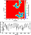 |
Fig. 8. Diffusion of CO on ASW. Panel A: Two-dimensional projection of CO interaction energy and diffusion path onto the ASW y − z plane from a simulation of 30 ns in length at 50 K. Panel B: One-dimensional projection of the path followed with some of the minima visited in panel A labeled with corresponding numbers. Between minima 15 and 17, the adsorbant repeatedly visits minima 8 to 17. The average diffusion barrier height is 1.15 kcal/mol compared with a range from 0.25 kcal/mol to 1.85 kcal/mol from experiments (Acharyya 2022; Karssemeijer & Cuppen 2014) |
The calculated average activation barrier for diffusion of NO (FigureA.10A) between neighboring minima is 0.91 kcal/mol with minimum and maximum barrier heights of 0.5 kcal/mol and 5.1 kcal/mol, respectively. From equilibrium trajectories at 50 K, no diffusion for CO2 and NO2 is observed on the 75 ns timescale. For CO2, one experiment reported an average diffusion barrier of 2150 K (4.3 kcal/mol) (He et al. 2018). As a comparison, for CO the average diffusion barrier height is ∼1 kcal/mol, which leads to a transition time between neighboring minima of ∼1 ns. Within an Arrhenius picture for surface diffusion –which may not be entirely appropriate at sufficiently low temperatures (Pezzella et al. 2018)– a barrier of ∼4 kcal/mol corresponds to a diffusion timescale on the order of several hundred nanoseconds. This is consistent with the present findings that CO2 does not diffuse on ASW on timescales of less than 100 ns. For comparison, the diffusion of CO2 and NO2 on the water surface after recombination is shown in Figure A.11.
Earlier work already demonstrated that computed oxygen diffusion coefficients are consistent with measurements. Atomic oxygen (Pezzella et al. 2018) on ASW experiences diffusional barriers ranging from Edif = 0.2 kcal/mol to 2 kcal/mol (100 K to 1000 K), compared with the average value of 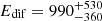 K determined from experiments (Minissale et al. 2016a).
4. Discussion and conclusions
The findings of the present work support the conclusion that larger molecules can form and stabilize on ASW from atomic and molecular constituents. The rate-limiting step for CO2 and NO2 generation is the diffusion of the reactant species. After recombination, both products efficiently cool on timescales of approximately 10 ps, although a smaller fraction still remains in an internally hot state. Use of a fluctuating charge model clarifies that, on the nanosecond timescale, recombination can occur from atom–molecule separations of up to at least ∼20 Å, which is much larger than the average separation between neighboring adsorption sites. This finding is in stark contrast to earlier work, which reported nonvanishing recombination probabilities only over a range of ∼5 Å due to using a simplified electrostatic model. Hence, it is concluded that recombination reactions for barrierless processes on ASW can occur on nanosecond timescales. It is also found that simplified models for the intramolecular energies, such as MMH, can yield qualitatively recombination probabilities, but are probably less suitable for studying energy relaxation because of the simplifications made. This is relevant when extending such studies to investigations of the formation of larger molecules for which construction of global and accurate machine-learning based PESs is still very challenging or even impossible (Unke & Meuwly 2019; Käser et al. 2023). Improved models, such as those based on MS-ARMD, provide viable future alternatives (Upadhyay et al. 2023).
Given the much longer timescales available in interstellar chemistry, the areas covered by the reactants will increase in proportion. The energy liberated upon recombination is efficiently transferred into water-internal modes and lattice vibrations (phonons) on picosecond timescales. Of particular note is the vanishingly small equilibrium diffusivity of CO2 and NO2 at low temperatures (here 50 K), which is consistent with experiments, whereas immediately after recombination the triatomics diffuse and roam wider parts of the ASW. For NO2, 11 % of the recombined trajectories show desorption in simulations of 1 ns in length, whereas no desorption is observed for CO2.
Astrophysical implications of the present work include physical and chemical aspects alike. Recombination reactions liberate energy to drive restructuring of the underlying surface. As a consequence of recombination, local heating of the ASW can take place, which also potentially increases the local diffusivity and leads to desorption of reactive species, such as H or OH. This is particularly relevant as the cold average temperatures (∼10 K) restrict translational motion to the lightest particles(Fredon et al. 2017). Because the morphology of a surface in part determines its chemical activity, reconfiguration of the solid support is an important determinant for downstream reactivity. Our simulations also show that following recombination, products undergo nonthermal surface diffusion (see Figure A.11), which leads to mass transport across the surface to initiate chemistry at other locations. This is particularly relevant because products can remain in an internally excited state, which can lead to breakup and radical formation.
In summary, the present work establishes that triatomics can be formed and stabilized following atom+diatom recombination reactions. The kernel-based potential energy surfaces combined with physically meaningful electrostatic models allow us to run statistically significant numbers of trajectories and provide molecular-level insight into energy relaxation and redistribution. This work provides a basis for broader reaction exploration on ASW, in particular in light of recent progress in representing high-dimensional, reactive PESs based on neural networks (Upadhyay et al. 2023).
Acknowledgments
The authors gratefully acknowledge financial support from the Swiss National Science Foundation through grant 200020_219779, the NCCR MUST, and AFOSR (all to MM). This article is based upon work from COST Action COSY CA21101, supported by COST (European Cooperation in Science and Technology).
References
- Acharyya, K. 2022, PASA, 39, e009 [NASA ADS] [CrossRef] [Google Scholar]
- Arakawa, E. T., & Nielsen, A. H. 1958, J. Mol. Spectrosc., 2, 413 [NASA ADS] [CrossRef] [Google Scholar]
- Bar-Nun, A., Dror, J., Kochavi, E., & Laufer, D. 1987, Phys. Rev. B, 35, 2427 [NASA ADS] [CrossRef] [Google Scholar]
- Bossa, J. B., Isokoski, K., de Valois, M. S., & Linnartz, H. 2012, A&A, 545, A82 [NASA ADS] [CrossRef] [EDP Sciences] [Google Scholar]
- Bossa, J.-B., Isokoski, K., Paardekooper, D. M., et al. 2014, A&A, 561, A136 [NASA ADS] [CrossRef] [EDP Sciences] [Google Scholar]
- Bossa, J.-B., Maté, B., Fransen, C., et al. 2015, ApJ, 814, 47 [NASA ADS] [CrossRef] [Google Scholar]
- Brooks, B., III, Brooks, C. L., Mackerell, A. D., Jr, et al. 2009, J. Comp. Chem., 30, 1545 [Google Scholar]
- Burnham, C. J., Li, J. C., & Leslie, M. 1997, J. Phys. Chem. B, 101, 6192 [NASA ADS] [CrossRef] [Google Scholar]
- Cazaux, S., Bossa, J.-B., Linnartz, H., & Tielens, A. G. G. M. 2015, A&A, 573, A16 [NASA ADS] [CrossRef] [EDP Sciences] [Google Scholar]
- Chaabouni, H., Minissale, M., Manicò, G., et al. 2012, J. Chem. Phys., 137, 234706 [NASA ADS] [CrossRef] [Google Scholar]
- Chou, S.-L., Lo, J.-I., Peng, Y.-C., et al. 2018, Phys. Chem. Chem. Phys., 20, 7730 [NASA ADS] [CrossRef] [Google Scholar]
- Christianson, D. A., & Garrod, R. T. 2021, Front. Astron. Space Sci., 8, 643297 [NASA ADS] [CrossRef] [Google Scholar]
- Codella, C., Viti, S., Lefloch, B., et al. 2018, MNRAS, 474, 5694 [NASA ADS] [CrossRef] [Google Scholar]
- Congiu, E., Fedoseev, G., Ioppolo, S., et al. 2012, ApJ, 750, L12 [NASA ADS] [CrossRef] [Google Scholar]
- de Barros, A., Da Silveira, E., Fulvio, D., Boduch, P., & Rothard, H. 2016, MNRAS, 465, 3281 [Google Scholar]
- Devlin, J. P. 1990, J. Mol. Struct., 224, 33 [NASA ADS] [CrossRef] [Google Scholar]
- Dulieu, F., Minissale, M., & Bockelée-Morvan, D. 2017, A&A, 597, A56 [NASA ADS] [CrossRef] [EDP Sciences] [Google Scholar]
- Ferrero, S., Pantaleone, S., Ceccarelli, C., et al. 2023, ApJ, 944, 142 [NASA ADS] [CrossRef] [Google Scholar]
- Fredon, A., Lamberts, T., & Cuppen, H. 2017, ApJ, 849, 125 [NASA ADS] [CrossRef] [Google Scholar]
- Frisch, M. J., Trucks, G. W., Schlegel, H. B., et al. 2016, Gaussian 16 Revision C.01 (Wallingford CT: Gaussian Inc.) [Google Scholar]
- Futrelle, R., & McGinty, D. 1971, Chem. Phys. Lett., 12, 285 [NASA ADS] [CrossRef] [Google Scholar]
- Gaigeot, M.-P., Martinez, M., & Vuilleumier, R. 2007, Mol. Phys., 105, 2857 [NASA ADS] [CrossRef] [Google Scholar]
- Galvez, O., Ortega, I. K., Maté, B., et al. 2007, A&A, 472, 691 [NASA ADS] [CrossRef] [EDP Sciences] [Google Scholar]
- Garstang, R. 1951, MNRAS, 111, 115 [CrossRef] [Google Scholar]
- Glendening, E. D., Landis, C. R., & Weinhold, F. 2012, Wiley Interdiscip. Rev. Comput. Mol. Sci., 2, 1 [Google Scholar]
- Hagen, W., Tielens, A., & Greenberg, 1981, J. Chem. Phys., 56, 367 [NASA ADS] [Google Scholar]
- Hama, T., & Watanabe, N. 2013, Chem. Rev., 113, 8783 [Google Scholar]
- Hama, T., Yokoyama, M., Yabushita, A., & Kawasaki, M. 2010, J. Chem. Phys., 133, 104504 [NASA ADS] [CrossRef] [Google Scholar]
- He, J., Acharyya, K., & Vidali, G. 2016, ApJ, 825, 89 [Google Scholar]
- He, J., Emtiaz, S., & Vidali, G. 2018, ApJ, 863, 156 [CrossRef] [Google Scholar]
- Herbst, E. 2001, Chem. Soc. Rev., 30, 168 [CrossRef] [Google Scholar]
- Ioppolo, S., Cuppen, H. M., & Linnartz, H. 2011, Rend. Lincei., 22, 211 [CrossRef] [Google Scholar]
- Ioppolo, S., Fedoseev, G., Minissale, M., et al. 2014, Phys. Chem. Chem. Phys., 16, 8270 [Google Scholar]
- Jenniskens, P., & Blake, D. 1994, Science, 265, 753 [NASA ADS] [CrossRef] [Google Scholar]
- Jorgensen, W. L., Chandrasekhar, J., Madura, J. D., Impey, R. W., & Klein, M. L. 1983, J. Chem. Phys., 79, 926 [Google Scholar]
- Karssemeijer, L., & Cuppen, H. 2014, A&A, 569, A107 [NASA ADS] [CrossRef] [EDP Sciences] [Google Scholar]
- Karssemeijer, L., Ioppolo, S., van Hemert, M., et al. 2013, ApJ, 781, 1 [Google Scholar]
- Käser, S., Vazquez-Salazar, L. I., Meuwly, M., & Töpfer, K. 2023, Digital Discov., 2, 28 [Google Scholar]
- Keane, J., Tielens, A., Boogert, A., Schutte, W., & Whittet, D. 2001, A&A, 376, 254 [NASA ADS] [CrossRef] [EDP Sciences] [Google Scholar]
- Kouchi, A., Furuya, K., Hama, T., et al. 2020, ApJ, 891, L22 [NASA ADS] [CrossRef] [Google Scholar]
- Kouchi, A., Tsuge, M., Hama, T., et al. 2021, ApJ, 918, 45 [NASA ADS] [CrossRef] [Google Scholar]
- Kumagai, N., Kawamura, K., & Yokokawa, T. 1994, Mol. Sim., 12, 177 [CrossRef] [Google Scholar]
- Lee, M. W., & Meuwly, M. 2011, J. Phys. Chem. A, 115, 5053 [NASA ADS] [CrossRef] [Google Scholar]
- Lee, M. W., & Meuwly, M. 2014, Faraday Discuss., 168, 205 [NASA ADS] [CrossRef] [Google Scholar]
- Ligterink, N. F. W., Calcutt, H., Coutens, A., et al. 2018, A&A, 619, A28 [NASA ADS] [CrossRef] [EDP Sciences] [Google Scholar]
- Liszt, H., & Turner, B. 1978, ApJ, 224, L73 [CrossRef] [Google Scholar]
- McGonagle, D., Ziurys, L., Irvine, W. M., & Minh, Y. 1990, ApJ, 359, 121 [NASA ADS] [CrossRef] [Google Scholar]
- Minissale, M., Congiu, E., Baouche, S., et al. 2013a, Phys. Rev. Lett., 111, 053201 [NASA ADS] [CrossRef] [Google Scholar]
- Minissale, M., Congiu, E., Manicò, G., Pirronello, V., & Dulieu, F. 2013b, A&A, 559, A49 [NASA ADS] [CrossRef] [EDP Sciences] [Google Scholar]
- Minissale, M., Fedoseev, G., Congiu, E., et al. 2014, Phys. Chem. Chem. Phys., 16, 8257 [Google Scholar]
- Minissale, M., Congiu, E., & Dulieu, F. 2016a, A&A, 585, A146 [NASA ADS] [CrossRef] [EDP Sciences] [Google Scholar]
- Minissale, M., Moudens, A., Baouche, S., Chaabouni, H., & Dulieu, F. 2016b, MNRAS, 458, 2953 [Google Scholar]
- Minissale, M., Nguyen, T., & Dulieu, F. 2019, A&A, 622, A148 [NASA ADS] [CrossRef] [EDP Sciences] [Google Scholar]
- Mizutani, Y., & Mizuno, M. 2022, J. Chem. Phys., 157, 240901 [Google Scholar]
- Molpeceres, G., Kästner, J., Fedoseev, G., et al. 2021, J. Phys. Chem. Lett., 12, 10854 [CrossRef] [Google Scholar]
- Nagy, T., Reyes, J. Y., & Meuwly, M. 2014, J. Chem. Theo. Comp., 10, 1366 [Google Scholar]
- Ndengué, S., Quintas-Sánchez, E., Dawes, R., & Osborn, D. 2021, J. Phys. Chem. A, 125, 5519 [CrossRef] [Google Scholar]
- Noble, J., Congiu, E., Dulieu, F., & Fraser, H. 2012, MNRAS, 421, 768 [NASA ADS] [Google Scholar]
- Oba, Y., Miyauchi, N., Hidaka, H., et al. 2009, ApJ, 701, 464 [NASA ADS] [CrossRef] [Google Scholar]
- Pezzella, M., & Meuwly, M. 2019, Phys. Chem. Chem. Phys., 21, 6247 [NASA ADS] [CrossRef] [Google Scholar]
- Pezzella, M., Unke, O. T., & Meuwly, M. 2018, J. Phys. Chem. Lett., 9, 1822 [CrossRef] [Google Scholar]
- Pezzella, M., Koner, D., & Meuwly, M. 2020, J. Phys. Chem. Lett., 11, 2171 [NASA ADS] [CrossRef] [Google Scholar]
- Plattner, N., & Meuwly, M. 2008, Chem. Phys. Chem.s, 9, 1271 [CrossRef] [Google Scholar]
- Qasim, D., Fedoseev, G., Chuang, K.-J., et al. 2020, Nat. Astron., 4, 781 [NASA ADS] [CrossRef] [Google Scholar]
- Romanzin, C., Ioppolo, S., Cuppen, H. M., van Dishoeck, E. F., & Linnartz, H. 2011, J. Chem. Phys., 134, 084504 [NASA ADS] [CrossRef] [Google Scholar]
- Roser, J. E., Vidali, G., Manicò, G., & Pirronello, V. 2001, ApJ, 555, L61 [NASA ADS] [CrossRef] [Google Scholar]
- Schmidt, F., Swiderek, P., & Bredehoöft, J. H. 2019, ACS Earth Space Chem., 3, 1974 [NASA ADS] [CrossRef] [Google Scholar]
- Shimanouchi, T., Matsuura, H., Ogawa, Y., & Harada, I. 1978, J. Phys. Chem. Ref. Data, 7, 1323 [NASA ADS] [CrossRef] [Google Scholar]
- Snyder, L. E., Kuan, Y.-J., Ziurys, L., & Hollis, J. 1993, ApJ, 403, L17 [CrossRef] [Google Scholar]
- Stief, L. J., Payne, W. A., & Klemm, R. B. 1975, J. Chem. Phys., 62, 4000 [NASA ADS] [CrossRef] [Google Scholar]
- Talbi, D., Chandler, G., & Rohl, A. 2006, Chem. Phys., 320, 214 [NASA ADS] [CrossRef] [Google Scholar]
- Truhlar, D. G., & Muckerman, J. T. 1979, Atom-Molecule Collision Theory (US: Springers), 505 [CrossRef] [Google Scholar]
- Tsuge, M., Hidaka, H., Kouchi, A., & Watanabe, N. 2020, ApJ, 900, 187 [Google Scholar]
- Unke, O. T., & Meuwly, M. 2017, J. Chem. Inf. Model., 57, 1923 [Google Scholar]
- Unke, O. T., & Meuwly, M. 2019, J. Chem. Theo. Comp., 15, 3678 [Google Scholar]
- Upadhyay, M., & Meuwly, M. 2021, ACS Earth Space Chem., 5, 3396 [CrossRef] [Google Scholar]
- Upadhyay, M., Pezzella, M., & Meuwly, M. 2021, J. Phys. Chem. Lett., 12, 6781 [CrossRef] [Google Scholar]
- Upadhyay, M., Topfer, K., & Meuwly, M. 2023, J. Phys. Chem. Lett., 15, 90 [Google Scholar]
- Vanommeslaeghe, K., & MacKerell, A. D. 2012, J. Chem. Inf. Model., 52, 3144 [Google Scholar]
- Veliz, J. C. S. V., Koner, D., Schwilk, M., Bemish, R. J., & Meuwly, M. 2020, Phys. Chem. Chem. Phys., 22, 3927 [NASA ADS] [CrossRef] [Google Scholar]
- Veliz, J. C. S. V., Koner, D., Schwilk, M., Bemish, R. J., & Meuwly, M. 2021, Phys. Chem. Chem. Phys., 23, 11251 [NASA ADS] [CrossRef] [Google Scholar]
- Wakelam, V., Bron, E., Cazaux, S., et al. 2017a, Mol. Astrophys., 9, 1 [Google Scholar]
- Wakelam, V., Loison, J.-C., Mereau, R., & Ruaud, M. 2017b, Mol. Astrophys., 6, 22 [NASA ADS] [CrossRef] [Google Scholar]
- Werner, H.-J., Knowles, P. J., Manby, F. R., et al. 2020, J. Chem. Phys., 152, 144107 [NASA ADS] [CrossRef] [Google Scholar]
- Yu, C.-C., Chiang, K.-Y., Okuno, M., et al. 2020, Nat. Commun., 11, 5977 [NASA ADS] [CrossRef] [Google Scholar]
- Ziurys, L., McGonagle, D., Minh, Y., & Irvine, W. 1991, ApJ, 373, 535 [CrossRef] [Google Scholar]
- Ziurys, L., Apponi, A., Hollis, J., & Snyder, L. 1994, ApJ, 436, L181 [NASA ADS] [CrossRef] [Google Scholar]
Appendix A: Appendix
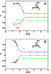 |
Fig. A.1. Change in charges of the atoms adsorbed to the 10 nearest H2O molecules for formation of CO2 (panel A) and NO2 (panel B) as a function of ρ (C–OB or N–OB) distance. At low temperatures, the reaction probability completely depends on the diffusion of species for which charges fit well at asymptotic. At close range (ρ ∼ 2 Å and shorter) bonded interactions dominate. Finally, at equilibrium, correct charges are achieved by the fitted function. Filled circles and solid line refers to ab initio determined and fitted charges, respectively. Color code: C and N atoms (blue) and atomic oxygen OB (red). |
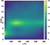 |
Fig. A.2. KDE density map for the average COO formation probability depending on initial (R, θ) using RKHS PES. |
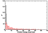 |
Fig. A.3. Normalized kinetic energy distribution for CO2 (red) and NO2 (black) from 280 reactive trajectories after 450 ps of recombination using RKHS PES. For NO2 ∼80 % of trajectories relaxed down to ∼5 kcal/mol whereas this fraction is only 40 % for CO2. In other words, upon recombination NO2 relaxes more effectively than CO2 on the sub-ns timescale. |
 |
Fig. A.4. The vibrational density of states power spectrum (black) and kinetic energy distribution (red) for water molecules A and B, WA (panel A) and WB (panel B), on the ASW surface at several delay times after the formation of CO2 using the MMH-PES. Panel C reports the vDOS and kinetic energy distribution for CO2. Top panel: Averaged vDOS spectrum and kinetic energy distribution from 10 randomly chosen surface water molecules from data before recombination takes place. Subsequent panels are labeled with the time interval after CO2 recombination. |
 |
Fig. A.5. Vibrational density of states power spectrum (in black) and P(Ekin) (red) for water molecules A and B, WA (panel A) and WB (panel B), on the ASW surface at several delay times after the formation of NO2 using the MMH-PES. Panel C reports the kinetic energy distribution (red) and the vDOS of the NO2 molecule. |
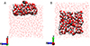 |
Fig. A.6. Side (left) and top (right) view of the ASW surface with CO2 on the top. The water molecules within 10 Å in the x−direction and 5 Å in the y − /z−directions are highlighted. |
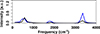 |
Fig. A.7. The vDOS spectrum for 10 randomly chosen surface water molecules (including WA and WB) before formation of CO2 (black, thermal equilibrium) and 120 ps after CO+O recombination (blue). The spectrum at t = 120 ps reproduces all features of the equilibrium vDOS, i.e. the system has returned to equilibrium on the 120 ps timescale. The intensities are “populations of modes within a given frequency interval”. |
 |
Fig. A.8. Time evolution of the integrated change of vDOS curves averaged over 100 water molecules for libration (black), bending (red), and stretching modes (green) of water using the MMH-PES. In Panel A, the equilibrium, thermally averaged area before recombination is the reference for calculating the difference at time t whereas for Panel B the peak area right after excitation (t = 1ps) is the reference. Here, solid lines represent the 4-point moving average. |
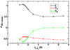 |
Fig. A.9. Fluctuating point charges from a natural bond order (NBO) analysis(Glendening et al. 2012). Calculations were carried out for the same snapshots as those in Figure A.1. However, NBO charges are yet larger in magnitude and increase the interaction between CO2 and the ASW which is inconsistent with experiments (Galvez et al. 2007; Wakelam et al. 2017b) |
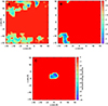 |
Fig. A.10. Interaction energy between the respective adsorbate and the ASW projected onto the y/z−plane from a 30 ns long simulation for NO (A), CO2 (B), and NO2 (C) on ASW at 50 K. Note that the color codes in panels A and B are the same but differ from that in panel C. |
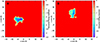 |
Fig. A.11. Diffusion of CO2 (Panel A) and NO2 (Panel B) on the water surface after recombination (XO+O → XO2) was observed in simulations running for 10 ns and 6 ns, respectively. This allows for comparison with the diffusion at 50 K, as shown in Figure A.10. |
Appendix B: Energy Transfer Using the MMH-PES
Using the MMH-PES one CO2-forming trajectory the kinetic energy distribution and vDOS of two water molecules WA and WB and the CO2 molecule were determined for windows 1 ps in length. The time of recombination was set to zero. Water molecules WA and WB were chosen according to the following criterion: for the first 9 ps, WA is the water molecule nearest to the newly formed CO2. At 9.1 ps, the CO2 molecule diffuses from one adsorption site on the ASW to a neighboring site which results in WB becoming the closest water molecule. As a reference point for the analysis, the averaged Ekin and vDOS for 10 water molecules located away from the recombination site was determined for the 0.5 ps prior to CO2-formation, see top row in Figure A.4.
For water molecule WA, the maximum of P(Ekin) (red shaded area) shifts to higher Ekin and its width increases considerably for the first 9 ps, after which relaxation to the thermal average is observed until 60 ps, see Figure A.4A. In contrast, P(Ekin) for WB (Figure A.4B) remains comparable to the thermal distribution for the first 8 ps after which the position of the maximum and the width increase. This is due to energy transfer between the partially relaxed CO2 molecule and WB after diffusion of the CO2. After 13 ps and until 60 ps the position of the maximum remains unchanged and the width of P(Ekin) decreases such that it reaches equilibrium again. As judged from the vDOS, the water stretch, bend and libration modes for WA and WB are populated for all time intervals. The two internal modes do not shift in frequency relative to the thermal equilibrium and their frequency is covered by the experimentally determined frequency range (Hagen & Tielens 1981; Yu et al. 2020; Devlin 1990).
The CO2 molecule formed is initially highly excited which leads to a broad, unstructured P(Ekin), top panel in Figure A.4C. Over the next 9 ps the width of P(Ekin) rapidly decreases due to energy exchange with WA and other surrounding water molecules and the phonon modes of the ASW. Cooling of CO2 continues after diffusion to the neighboring site and within 60 ps after recombination the P(Ekin) for CO2 is comparable to that of the surrounding water molecules. For the vDOS of CO2 a rather different picture emerges than for water. The measured (Shimanouchi et al. 1978) vibrational frequencies for CO2 are at 667 (bend), 1333 (symmetric stretch), 2349 (antisymmetric stretch) cm−1 (see dashed vertical lines) and at 647, 1374, 2353 cm−1 from calculations using the reactive PES, which is in reasonably good agreement with experiment. At the end of the observation window at 60 ps the three modes are clearly visible. However, for times shortly after recombination only frequencies below ∼1000 cm−1 appear in the vDOS.
For studying energy transfer between neighboring water molecules on the ASW, a slightly different approach was used for NO2 recombination. Again, P(Ekin) and the vDOS of water molecules WA and WB and NO2 were determined for one NO2−forming trajectory on the MMH PES. Here, WA is the water molecule closest to NO2, while WB is hydrogen-bonded to WA, see Figure A.5. For the first 1 ps after recombination the widths of P(Ekin) for WA and WB are considerably broader than the thermal distribution, see top panel in Figure A.5A. Energy exchange between the two water molecules is readily observed for the following 5 ps with maxima and widths of P(Ekin) increasing and decreasing. The distributions for 10 ps and 40 ps do not change appreciably anymore and the two water molecules do not fully thermalize on that time scale. The kinetic energy distribution for NO2 starts out broad (50 kcal/mol) and transfers more than half of this energy to the environment within 10 ps of recombination (Figure A.5C).
The experimentally measured(Arakawa & Nielsen 1958) vibrational frequencies for gas phase NO2 are at 750 (bend), 1318 (symmetric stretch), 1618 (antisymmetric stretch) cm−1. A blue shift over time is observed as the NO2 molecule loses energy. After 60 ps, it begins to probe the low-energy regions of the potential, revealing distinct peaks. For NO2, the final Ekin fluctuates around ∼5 kcal/mol, causing the peak to shift from its equilibrium features. During the initial picoseconds, there is a notable population in the region of the water libration modes compared to bending and stretching. However beyond 60 ps, as the system approaches equilibrium, the range of the libration modes is less populated/unpopulated. In contrast, the stretching modes gain intensity.
All Figures
|
Fig. 1. Simulation system for studying CO2 (panel A) and NO2 (panel B) recombination. Panel A color code: Oxygen (red), CO (cyan), CO2 (orange). Panel B color code: Oxygen (red), NO (blue), NO2 (yellow). Before and after recombination, all species diffuse on the ASW. |
| In the text | |
|
Fig. 2. Recombination of CO + O to form CO2 (left column) and NO + O to NO2 (right column) in ground state. Panels A and D: OB–C/N (red) and OA–C/N (black) separation. Panels B and E: O–C/N–O angle. Panels C and F: Temperature of the ASW (cyan) and the full system (black) before and after recombination. Upon recombination, both O–C/N stretches exhibit equally pronounced excitation (shown in the insets). |
| In the text | |
|
Fig. 3. KDE density map for the average CO2 formation probability depending on initial (R, θ) using the MMH (Panel A) and RKHS (Panel B) PES. The color palette indicates the probability of the reaction, with yellow representing P = 1 and blue representing P = 0. The COO formation probability using RKHS PES is shown in Figure A.2. |
| In the text | |
|
Fig. 4. NO2 formation probability as a function of R and θ using MMH (Panel A) and RKHS (Panel B) PES. The color palette indicates the probability of the reaction, with yellow representing P = 1 and blue representing P = 0. |
| In the text | |
|
Fig. 5. Vibrational density of states power spectrum (in black) and P(Ekin) (red) for water molecules A and B, WA (panel A) and WB (panel B), on the ASW surface at several delay times after the formation of CO2 on the RKHS-PES. The IR bands at 1600 − 1750 and 3200 − 3600 cm−1 correspond to bending and OH-stretching modes (Hagen & Tielens 1981; Yu et al. 2020; Devlin 1990). Panel C reports the kinetic energy distribution (red) and the vDOS of the CO2 molecule. Top panel: Averaged vDOS spectrum and kinetic energy distribution for ten water molecules away from the recombination site determined for the 0.5 ps prior to CO2 formation. Subsequent panels are labeled with the time interval after CO2 recombination. See Figure A.4 for an analysis of a trajectory using the MMH PES. |
| In the text | |
|
Fig. 6. Vibrational density of states power spectrum (in black) and P(Ekin) (red) for water molecules A and B, WA (panel A) and WB (panel B), on the ASW surface at several delay times after the formation of NO2 on the RKHS-PES. The IR bands at 1600 − 1750 and 3200 − 3600 cm−1 correspond to bending and OH-stretching modes (Hagen & Tielens 1981; Yu et al. 2020; Devlin 1990). Panel C reports the kinetic energy distribution (red) and the vDOS of the NO2 molecule. For an analysis of a trajectory using the MMH PES, see Figure A.5. |
| In the text | |
|
Fig. 7. Time evolution of the integrated change of vDOS curves averaged over 100 water molecules for libration (black), bending (red), and stretching modes (green) of water using the RKHS-PES. In panel A, the equilibrium, thermally averaged area before recombination is the reference for calculating the difference at time t, whereas for panel B, the peak area immediately after excitation (t = 1ps) is the reference. Here, solid lines represent the four-point moving average. For an analysis using the MMH PES, see Figure A.8. |
| In the text | |
|
Fig. 8. Diffusion of CO on ASW. Panel A: Two-dimensional projection of CO interaction energy and diffusion path onto the ASW y − z plane from a simulation of 30 ns in length at 50 K. Panel B: One-dimensional projection of the path followed with some of the minima visited in panel A labeled with corresponding numbers. Between minima 15 and 17, the adsorbant repeatedly visits minima 8 to 17. The average diffusion barrier height is 1.15 kcal/mol compared with a range from 0.25 kcal/mol to 1.85 kcal/mol from experiments (Acharyya 2022; Karssemeijer & Cuppen 2014) |
| In the text | |
|
Fig. A.1. Change in charges of the atoms adsorbed to the 10 nearest H2O molecules for formation of CO2 (panel A) and NO2 (panel B) as a function of ρ (C–OB or N–OB) distance. At low temperatures, the reaction probability completely depends on the diffusion of species for which charges fit well at asymptotic. At close range (ρ ∼ 2 Å and shorter) bonded interactions dominate. Finally, at equilibrium, correct charges are achieved by the fitted function. Filled circles and solid line refers to ab initio determined and fitted charges, respectively. Color code: C and N atoms (blue) and atomic oxygen OB (red). |
| In the text | |
|
Fig. A.2. KDE density map for the average COO formation probability depending on initial (R, θ) using RKHS PES. |
| In the text | |
|
Fig. A.3. Normalized kinetic energy distribution for CO2 (red) and NO2 (black) from 280 reactive trajectories after 450 ps of recombination using RKHS PES. For NO2 ∼80 % of trajectories relaxed down to ∼5 kcal/mol whereas this fraction is only 40 % for CO2. In other words, upon recombination NO2 relaxes more effectively than CO2 on the sub-ns timescale. |
| In the text | |
|
Fig. A.4. The vibrational density of states power spectrum (black) and kinetic energy distribution (red) for water molecules A and B, WA (panel A) and WB (panel B), on the ASW surface at several delay times after the formation of CO2 using the MMH-PES. Panel C reports the vDOS and kinetic energy distribution for CO2. Top panel: Averaged vDOS spectrum and kinetic energy distribution from 10 randomly chosen surface water molecules from data before recombination takes place. Subsequent panels are labeled with the time interval after CO2 recombination. |
| In the text | |
|
Fig. A.5. Vibrational density of states power spectrum (in black) and P(Ekin) (red) for water molecules A and B, WA (panel A) and WB (panel B), on the ASW surface at several delay times after the formation of NO2 using the MMH-PES. Panel C reports the kinetic energy distribution (red) and the vDOS of the NO2 molecule. |
| In the text | |
|
Fig. A.6. Side (left) and top (right) view of the ASW surface with CO2 on the top. The water molecules within 10 Å in the x−direction and 5 Å in the y − /z−directions are highlighted. |
| In the text | |
|
Fig. A.7. The vDOS spectrum for 10 randomly chosen surface water molecules (including WA and WB) before formation of CO2 (black, thermal equilibrium) and 120 ps after CO+O recombination (blue). The spectrum at t = 120 ps reproduces all features of the equilibrium vDOS, i.e. the system has returned to equilibrium on the 120 ps timescale. The intensities are “populations of modes within a given frequency interval”. |
| In the text | |
|
Fig. A.8. Time evolution of the integrated change of vDOS curves averaged over 100 water molecules for libration (black), bending (red), and stretching modes (green) of water using the MMH-PES. In Panel A, the equilibrium, thermally averaged area before recombination is the reference for calculating the difference at time t whereas for Panel B the peak area right after excitation (t = 1ps) is the reference. Here, solid lines represent the 4-point moving average. |
| In the text | |
|
Fig. A.9. Fluctuating point charges from a natural bond order (NBO) analysis(Glendening et al. 2012). Calculations were carried out for the same snapshots as those in Figure A.1. However, NBO charges are yet larger in magnitude and increase the interaction between CO2 and the ASW which is inconsistent with experiments (Galvez et al. 2007; Wakelam et al. 2017b) |
| In the text | |
|
Fig. A.10. Interaction energy between the respective adsorbate and the ASW projected onto the y/z−plane from a 30 ns long simulation for NO (A), CO2 (B), and NO2 (C) on ASW at 50 K. Note that the color codes in panels A and B are the same but differ from that in panel C. |
| In the text | |
|
Fig. A.11. Diffusion of CO2 (Panel A) and NO2 (Panel B) on the water surface after recombination (XO+O → XO2) was observed in simulations running for 10 ns and 6 ns, respectively. This allows for comparison with the diffusion at 50 K, as shown in Figure A.10. |
| In the text | |
Current usage metrics show cumulative count of Article Views (full-text article views including HTML views, PDF and ePub downloads, according to the available data) and Abstracts Views on Vision4Press platform.
Data correspond to usage on the plateform after 2015. The current usage metrics is available 48-96 hours after online publication and is updated daily on week days.
Initial download of the metrics may take a while.