| Issue |
A&A
Volume 688, August 2024
|
|
|---|---|---|
| Article Number | A81 | |
| Number of page(s) | 18 | |
| Section | Planets and planetary systems | |
| DOI | https://doi.org/10.1051/0004-6361/202450328 | |
| Published online | 06 August 2024 | |
Population synthesis models indicate a need for early and ubiquitous disk substructures
1
University Observatory, Faculty of Physics, Ludwig-Maximilians-Universität München,
Scheinerstr. 1,
81679
Munich,
Germany
e-mail: This email address is being protected from spambots. You need JavaScript enabled to view it.
2
Exzellenzcluster ORIGINS,
Boltzmannstr. 2,
85748
Garching,
Germany
3
European Southern Observatory,
Karl-Schwarzschild-Strasse 2,
85748
Garching bei München,
Germany
4
Mullard Space Science Laboratory, University College London, Holmbury St Mary,
Dorking, Surrey
RH5 6NT,
UK
5
Dipartimento di Fisica ‘Aldo Pontremoli’, Università degli Studi di Milano,
via G. Celoria 16,
20133
Milano,
Italy
6
Center for Astrophysics | Harvard & Smithsonian,
60 Garden St.,
Cambridge,
MA
02138,
USA
Received:
11
April
2024
Accepted:
19
May
2024
Abstract
Context. Large millimeter surveys of star-forming regions enable the study of entire populations of planet-forming disks and reveal correlations between their observable properties. The ever-increasing number of these surveys has led to a flourishing of population study, a valuable tool and approach that is spreading in ever more fields. Population studies of disks have shown that the correlation between disk size and millimeter flux could be explained either through disks with strong substructure, or alternatively by the effects of radial inward drift of growing dust particles.
Aims. This study aims to constrain the parameters and initial conditions of planet-forming disks and address the question of the need for the presence of substructures in disks and, if needed, their predicted characteristics, based on the large samples of disk sizes, millimeter fluxes, and spectral indices available.
Methods. We performed a population synthesis of the continuum emission of disks, exploiting a two-population model (two-pop-py), considering the influence of viscous evolution, dust growth, fragmentation, and transport, varying the initial conditions of the disk and substructure to find the best match with the observed distributions. Disks both with and without substructure have been examined. We obtained the simulated population distribution for the disk sizes, millimeter fluxes, and spectral indices by post-processing the resulting disk profiles (surface density, maximum grain size, and disk temperature).
Results. We show that the observed distributions of spectral indices, sizes, and luminosities together can be best reproduced by disks with significant substructure; namely, a perturbation that is strong enough to be able to trap particles, that is formed early in the evolution of the disk, and that is within 0.4 Myr. Agreement is reached by relatively high initial disk masses (10−2.3 M⋆ ⩽ Mdisk ⩽ 10−0.5 M⋆) and moderate levels of turbulence (10−3.5 ⩽ α ⩽ 10−2.5). Other disk parameters play a weaker role. Only opacities with a high absorption efficiency can reproduce the observed spectral indices.
Conclusions. Disk population synthesis is a precious tool for investigating and constraining the parameters and initial conditions of planet-forming disks. The generally low observed spectral indices call for significant substructure, like that which planets in the mass range of Saturn to a few Jupiters would induce, to already be present before 0.4 Myr. Our results indicate that substructure, which so far has only been assessed in individual disks, is likely ubiquitous and extends to the whole population, and imply that most “smooth” disks hide unresolved substructure.
Key words: protoplanetary disks
© The Authors 2024
 Open Access article, published by EDP Sciences, under the terms of the Creative Commons Attribution License (https://creativecommons.org/licenses/by/4.0), which permits unrestricted use, distribution, and reproduction in any medium, provided the original work is properly cited.
This article is published in open access under the Subscribe to Open model. This email address is being protected from spambots. You need JavaScript enabled to view it. to support open access publication.
1 Introduction
The advent of the Atacama Large Millimeter/submillimeter Array (ALMA) has strongly revolutionized the protoplanetary disk field. High-resolution observations have shown that most disks that have been imaged are characterized by the presence of substructures (Andrews et al. 2018a; Huang et al. 2018; Long et al. 2018). Different mechanisms have been proposed to explain the origin of substructures in protoplanetary disks, such as planets (e.g., Rice et al. 2006; Paardekooper & Mellema 2004; Pinilla et al. 2012a), magnetohydrodynamics (MHD) processes (Johansen et al. 2009; Bai & Stone 2014), binary companions (Shi et al. 2012; Ragusa et al. 2017, e.g.), or variations in dust material properties (e.g., Birnstiel et al. 2010; Okuzumi et al. 2016; Pinilla et al. 2017). Nevertheless, it is widely believed that the presence of planets or protoplanets could be the reason behind the substructures observed in Class II disks, mainly due to kinematic evidence (Teague et al. 2018; Pinte et al. 2018; Izquierdo et al. 2022) or directly imaged planets within the gaps, as in the case of PDS70 (Müller et al. 2018; Keppler et al. 2018). However, there is still a need to connect the distribution of exoplanets observed to a potential planet population in protoplanetary disks.
High-resolution observations enable individual disks to be studied and characterized in great detail. However, these observations tend to be biased toward the brightest and largest disks. Nevertheless, ALMA has also been revolutionary in enabling large samples of lower-resolution observations. These observations have provided hundreds of disks in large sample surveys of entire star-forming regions (see Manara et al. 2023, for a recent review), and have uncovered the existence of correlations between several disk-star observables such as the disk size–luminosity relation (SLR) (Tripathi et al. 2017; Andrews et al. 2018b), Mdust − Mstar (Andrews et al. 2013; Ansdell et al. 2016; Pascucci et al. 2016), ![Mathematical equation: $\[\dot{M}\]$](/articles/aa/full_html/2024/08/aa50328-24/aa50328-24-eq1.png) – Mdust (Manara et al. 2016), and the distribution of several key parameters of disks, such as the disk spectral index (Ricci et al. 2010a,b; Tazzari et al. 2021a).
– Mdust (Manara et al. 2016), and the distribution of several key parameters of disks, such as the disk spectral index (Ricci et al. 2010a,b; Tazzari et al. 2021a).
Surveys have thus opened up a new range of questions that cannot be answered by studying individual disks: what are the key mechanisms at play during the evolution of the disks that are needed to reproduce the distributions at different disk ages and the observed correlations? What mechanisms are responsible for the transport of angular momentum in disks (viscosity or MHD winds)? What are the initial conditions of the protoplanetary disks that are needed to reproduce observations? Surveys have thus led to the need to find models that can reproduce what we observe. Disk population synthesis is the tool of choice to study these questions. Simulating thousands of models of protoplanetary disks evolving for several million years, disk population synthesis enables disk initial conditions to be constrained and the identification of key evolutionary mechanisms of protoplanetary disks by comparing the results obtained with the simulations to the large number of surveys available.
This study represents an extension of the study performed by Zormpas et al. (2022). They explored whether smooth disks and substructured disks can reproduce the SLR, performing a disk population study. In particular, they showed that smooth disks in the drift regime correctly reproduce the observed SLR (see also Rosotti et al. 2019a). However, their study has also shown that substructured disks can populate the bright part of the SLR, despite following a different relation. Thus, they state that the observed sample could be composed of a mixture of smooth and substructured disks. The performed disk population study has also exhibited the need to have a high initial disk mass and low turbulence to reproduce the observed distribution. Finally, they have shown that grain composition and porosity play a key role in the evolution of disks in the size–luminosity diagram. In particular, the opacity model from Ricci et al. (2010b) but with compact grains, as in Rosotti et al. (2019a), has been proven to better reproduce the SLR than the Disk Substructures at High Angular Resolution Project (DSHARP) opacities (Birnstiel et al. 2018, which are similar in composition to previously used opacities such as those in Pollack et al. 1994 or D’Alessio et al. 2006). A similar indication concerning DSHARP opacities comes from the study of Stadler et al. (2022), which shows that the opacity model of Ricci et al. (2010b) leads to a better matching of the observed spectral index, in contrast to DSHARP opacities.
In this study, we aim to extend the work of Zormpas et al. (2022) by exploring whether smooth and substructured disks can reproduce the observed spectral index distribution, and we explore the required initial conditions that lead to evolved disks matching current observations. Moreover, we aim to understand whether it is possible to match both the size–luminosity and spectral index distributions at the same time and which initial disk parameters are required for that.
This paper is structured as follows: in Sec. 2, we describe our computational model for the evolution of the disk and introduce the analysis method we used to compare this to disk observations. Section 3 introduces the main results obtained and the comparison with the observed distributions. We first focus on reproducing the spectral index and then on the possibility of a simultaneous matching of both the spectral index and the size–luminosity distributions. Section 4 presents our conclusions.
2 Methods
The two-population model (two-pop-py) by Birnstiel et al. (2012, 2015) has been exploited to perform 1D simulations to describe the gas and dust evolution in the disk. Two-pop-py is a tool that is well suited for disk population studies since it captures the dust surface density evolution, the viscous evolution of the gas, and the particle size with good accuracy. Being based on a set of simple equations, it allows one to perform a single simulation quickly (in a matter of seconds), making it computationally feasible to run large numbers of simulations within a reasonable amount of time. In the following, we describe the main characteristics of the two-pop-py model and the assumptions on which it is based.
2.1 Disk evolution
The protoplanetary gas disk was evolved according to the viscous disk evolution equation (Lüst 1952; Lynden-Bell & Pringle 1974), using the turbulent effective viscosity parameterized in (Shakura & Sunyaev 1973),
![Mathematical equation: $\[\nu=\alpha_{\mathrm{gas}} \frac{c_{\mathrm{s}}^2}{\Omega_k};\]$](/articles/aa/full_html/2024/08/aa50328-24/aa50328-24-eq2.png) (1)
(1)
the dust diffusion coefficient is
![Mathematical equation: $\[D \simeq \alpha_{\text {dust }} \frac{c_{\mathrm{s}}^2}{\Omega_k},\]$](/articles/aa/full_html/2024/08/aa50328-24/aa50328-24-eq3.png) (2)
(2)
where αgas, cs, and Ωk denote the turbulence parameter, the sound speed, and the Keplerian frequency, respectively. The additional term ![Mathematical equation: $\[\frac{1}{1+\mathrm{St}^2}\]$](/articles/aa/full_html/2024/08/aa50328-24/aa50328-24-eq4.png) , with St being the Stokes number, derived in Youdin & Lithwick (2007), was dropped since the Stokes number is always <1 in all the simulations that have been performed.
, with St being the Stokes number, derived in Youdin & Lithwick (2007), was dropped since the Stokes number is always <1 in all the simulations that have been performed.
As in Zormpas et al. (2022), two different families of disk models have been taken into account in our study: smooth disks and substructured disks. A smooth disk is characterized by the absence of any gaps during its entire evolution, while a substructured disk is a disk in which a single substructure is created during its evolution. In contrast to Zormpas et al. (2022), in which substructure is inserted from the beginning of the evolution of the disk, our substructured disk starts as a smooth disk and during its evolution a gap is created, and thus the disk becomes substructured. This new approach allows one to investigate the effect of the time at which substructure is inserted during the evolution of the system. The substructure was modeled as a gap due to the presence of a planet that was inserted in the disk. To mimic the presence of a planetary gap, we subdivided the α parameter into two different values: αgas and αdust. The presence of the planet was modeled as a local variation in the gas viscosity, while other than in the proximity of the gap, the two parameters were taken to be identical; that is, αgas = αdust. More information on how we modeled the planet’s presence in the disk can be found in Sec. 2.3. Adopting the two-population model described in Birnstiel et al. (2012), we evolved the dust surface density, assuming that the small dust is tightly coupled to the gas, while the large dust particles can decouple from it and drift inward. The initial gas surface density follows the Lynden-Bell & Pringle (1974) self-similar solution,
![Mathematical equation: $\[\Sigma_{\mathrm{g}}(r)=\Sigma_0\left(\frac{r}{r_{\mathrm{c}}}\right)^{-\gamma} \exp \left[-\left(\frac{r}{r_{\mathrm{c}}}\right)^{2-\gamma}\right],\]$](/articles/aa/full_html/2024/08/aa50328-24/aa50328-24-eq5.png) (3)
(3)
where the normalization parameter, ![Mathematical equation: $\[\Sigma_0=(2-\gamma) M_{\text {disk }} / 2 \pi r_{\mathrm{c}}^2\]$](/articles/aa/full_html/2024/08/aa50328-24/aa50328-24-eq6.png) , is set by the initial disk mass, Mdisk, rc denotes the so-called characteristic radius of the disk, and γ denotes the viscosity exponent. For our simulations, γ was set to 1 for the initial profiles of all the disks. This choice is mostly consistent with our choice of viscosity (see Eq. (1)), which deviates from γ = 1 only in the case of substructure being included and in the isothermal part of the disk. Furthermore, choosing γ ≠ 1 would relax back to the γ = 1 case on a viscous timescale. The initial dust surface density is related to the gas surface density by a constant initial dust-to-gas ratio of ∑d/∑g = 0.01.
, is set by the initial disk mass, Mdisk, rc denotes the so-called characteristic radius of the disk, and γ denotes the viscosity exponent. For our simulations, γ was set to 1 for the initial profiles of all the disks. This choice is mostly consistent with our choice of viscosity (see Eq. (1)), which deviates from γ = 1 only in the case of substructure being included and in the isothermal part of the disk. Furthermore, choosing γ ≠ 1 would relax back to the γ = 1 case on a viscous timescale. The initial dust surface density is related to the gas surface density by a constant initial dust-to-gas ratio of ∑d/∑g = 0.01.
The two-population model consists of a population of the initial grain size amin = 0.1 μm, the size of which is kept constant in time and space during the evolution, and a large grain population that is allowed to increase in size with time. When Ricci et al. (2010b) opacities had been taken into account, the particle bulk density was set to a value of ρs = 1.7 g cm−3 as we considered the composition of Ricci et al. (2010b) but for the case of compact grains (no porosity), as in the model of Rosotti et al. (2019a). These opacities are henceforth referred to as “Ricci compact opacities”. For DSHARP (Birnstiel et al. 2018) opacities, we set ρs = 1.675 g cm−3 (0% porosity case), and this value decreases based on the porosity assumed for the grains. The grain composition consists of 60% water ice, 30% carbonaceous materials, and 10% silicates by volume. For DIANA (Woitke et al. 2016) opacities, we set ρs = 2.08 g cm−3. For a comparison with the size–luminosity distribution observed by Andrews et al. (2018b), we computed the opacity in ALMA Band 7, more precisely at 0.89 mm, and as is described in Sec. 2.4 we evaluated the continuum intensity profile of the disk, considering the absorption and scattering opacity contributions (see Sec. 2.4). Four different grain porosity cases have been explored for the DSHARP opacity model (Birnstiel et al. 2018): 0%, 10%, 50%, and 90% porosity. The bulk densities adopted for these four cases are the following: ρs = 1.675 g cm−3, ρs = 1.508 g cm−3, ρs = 0.838 g cm−3, and ρs = 0.168 g cm−3. Ricci compact opacities were adopted as the standard case in our analysis. When another model was adopted, this is specified. For each simulation, the disk has evolved for 3 Myr.
The 1D disk was spatially modeled with a radial grid that ranges from 0.05 au to 2000 au, and the cells of the grid were spaced logarithmically. The main characteristics of the grid model are reported in Table 1.
The temperature of the disk was linked to the luminosity of the star; that is, we worked within an adaptive temperature scenario. However, both the stellar luminosity, L⋆, and the effective temperature, T, are not evolved in our simulations. In Appendix A, we show a comparison with the scenario in which L⋆, and thus T, evolve, showing that the results are analogous to the fixed scenario.
We adopted a passive irradiated disk temperature model; no viscous heating or other processes were considered. In particular, we followed the temperature profile adopted by Kenyon et al. (1996):
![Mathematical equation: $\[T=\left(\phi \frac{L_{\star}}{4 \pi \sigma_{S~B} r^2}+(10 K)^4\right)^{1 / 4},\]$](/articles/aa/full_html/2024/08/aa50328-24/aa50328-24-eq7.png) (4)
(4)
where L⋆ is the star luminosity, σS B the Stefan-Boltzmann constant, and ϕ the flaring angle, set to 0.05. The floor temperature of the disk was set to 10 K. The star’s luminosity value, L⋆, was set starting from the star’s mass value, M⋆, exploiting Siess et al. (2000) evolutionary tracks and considering the value of L⋆ when the star has an age of 1 Myr. M⋆ was set based on the initial mass function (IMF) of Chabrier and Kroupa (see next Sec. 2.2).
Fixed parameters.
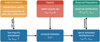 |
Fig. 1 Disk population study procedure. |
2.2 Disk population synthesis
Disk population synthesis is based on the idea of performing a large number of simulations of the evolution of dust and gas over millions of years, to constrain disk initial conditions and identify which key mechanisms are at play in the disk by comparing the distribution of the observable parameters obtained from the simulations with the observed ones.
Figure 1 explains the key idea behind our disk population study. Firstly, a large set of initial parameters was set up, combining different initial values of the main parameters used to describe each disk. In particular, to map all the parameter space, the set of initial conditions adopted for each disk was constructed by randomly drawing each parameter from a probability distribution function (PDF). A total of 105 simulations were performed for each population synthesis; these map well the entire relevant parameter space. The main parameters that were taken into account to describe the disk are: disk mass (Mdisk), stellar mass (M⋆), disk characteristic radius (rc), viscous parameter (α), and fragmentation velocity (υfrag). This choice of parameters applies to the description of all the disks (i.e., both smooth and sub-structured disks). Substructured disks are characterized by three additional parameters: the mass of the planet that creates the gap (mp), the time (tp), and the position (rp) at which the planet was inserted. This set of three additional parameters applies to each planet that is inserted in the system; that is, in the extra cases of double substructured systems (see Sec. 3.2), each gap has been characterized by its own set of three parameters (mp,i, tp,i, rp,i). The drawing of the mp value was performed after drawing a value of Mdisk, to impose the further physically reasonable restriction of mp < Mdisk. In the case of multiple substructures, we applied the following constraint: ∑i mp,i < Mdisk. Table 2 shows the range that has been adopted for each parameter.
The viscosity parameter, α, and the initial mass of the disk, Mdisk, were randomly drawn from a log uniform PDF to uniformly span the full range of values adopted for these two parameters. A log uniform PDF was adopted for the disk characteristic radius, rc, too, to resemble the observed behavior of the protoplanetary disks’ sizes. The values of the stellar mass, M⋆, were drawn from a functional form of the IMF proposed by Maschberger (2013), which is based on the standard IMFs of Kroupa (Kroupa 2001, 2002) and Chabrier (Chabrier 2003).
Given the set of 105 initial conditions, each disk was evolved for 3 Myr using the two-pop-py evolutionary code. For the evolved disks obtained through two-pop-py, we evaluated the observables parameters (Sects. 2.4 and 2.5). Finally, the distributions of the observable parameters obtained for the simulated disks were compared to the observed ones.
Both the observed and simulated fluxes of each disk were scaled to a reference distance of 140 pc.
Disk initial parameters.
2.3 Planetary gaps
The substructured disks were produced by generating a gap through the insertion of a planet during the evolution of the disk. The presence of a massive planet in the disk leads to the formation of a gap in the gas distribution, which we call substructure. To mimic the gap associated with a planet’s presence in our disks, we modified the value of the αgas parameter. We took advantage of the inverse proportionality between αgas and ∑g in a steady state regime; that is, αgas ∝ 1/∑g. Thus, a bump in the αgas profile will reflect in a gap in the ∑g profile that reproduces the presence of a planetary gap; besides, this procedure allows one to keep a viscous evolution for ∑g. We adopted the Kanagawa et al. (2016) prescription to model the gap created by a given planet at a given position in the disk.
The main parameter that describes the gap formed by the planet is
![Mathematical equation: $\[K=\left(\frac{M_{\mathrm{p}}}{M_{\star}}\right)^2\left(\frac{h_{\mathrm{p}}}{R_{\mathrm{p}}}\right)^{-5} \alpha^{-1}.\]$](/articles/aa/full_html/2024/08/aa50328-24/aa50328-24-eq8.png) (5)
(5)
The main caveat associated with the Kanagawa prescription is that it is an analytical approximation of the gap depth and width. However, as is described in Zormpas et al. (2022), the width of the gap is the dominant factor in the evolution of the disk, and the depth is not crucial to the evolution of the disk. The position and radial extent of the gap are what matter the most to the evolution of the disk and those are well reproduced by the prescription.
2.4 Observables
One of the problems when dealing with protoplanetary disks is defining their size (see Miotello et al. 2023, as a review). Indeed, as is discussed in Tripathi et al. (2017) and Rosotti et al. (2019b), we cannot adopt the characteristic radius, rc, as a size indicator of the disks. We thus followed the procedure of defining an effective radius, reff, of the disk. The effective radius is defined as the radius that encompasses a given fraction of the total amount of flux that is produced by the disk. We chose to define our effective radius as the radius that encloses the 68% of the total amount of flux produced by the disk, following Tripathi et al. (2017).
The Miyake & Nakagawa (1993) scattering solution of the radiative transfer equation was adopted to evaluate the mean intensity, Jν:
![Mathematical equation: $\[\frac{J_\nu\left(\tau_\nu\right)}{B_\nu(T(r))}=1-b\left(\mathrm{e}^{-\sqrt{3 \epsilon_\nu^{\text {elf }}}\left(\frac{1}{2} \Delta \tau-\tau_\nu\right)}+\mathrm{e}^{-\sqrt{3 \epsilon_\nu^{\text {eff }}}\left(\frac{1}{2} \Delta \tau+\tau_\nu\right)}\right),\]$](/articles/aa/full_html/2024/08/aa50328-24/aa50328-24-eq9.png) (6)
(6)
where Bν is the Planck function and
![Mathematical equation: $\[b=\left[\left(1-\sqrt{\epsilon_\nu^{\text {eff }}}\right) \mathrm{e}^{-\sqrt{3 \epsilon_\nu^{\text {eff }}} \Delta \tau}+1+\sqrt{\epsilon_\nu^{\text {eff }}}\right]^{-1},\]$](/articles/aa/full_html/2024/08/aa50328-24/aa50328-24-eq10.png) (7)
(7)
and the optical depth, τν, is given by
![Mathematical equation: $\[\tau_\nu=\left(k_\nu^{\mathrm{abs}}+k_\nu^{\mathrm{sca}, \mathrm{eff}}\right) \Sigma_{\mathrm{d}},\]$](/articles/aa/full_html/2024/08/aa50328-24/aa50328-24-eq11.png) (8)
(8)
where
![Mathematical equation: $\[k_\nu^{\text {sca,eff }}=\left(1-g_\nu\right) k_\nu^{\text {sca}}\]$](/articles/aa/full_html/2024/08/aa50328-24/aa50328-24-eq12.png) (9)
(9)
is the effective scattering opacity and ![Mathematical equation: $\[k_\nu^{\text {abs }}\]$](/articles/aa/full_html/2024/08/aa50328-24/aa50328-24-eq13.png) is the dust absorption opacity, obtained from the Ricci compact (Rosotti et al. 2019a), DSHARP (Birnstiel et al. 2018), or DIANA (Woitke et al. 2016) opacities. gν is the forward scattering parameter. The introduction of the effective scattering opacity,
is the dust absorption opacity, obtained from the Ricci compact (Rosotti et al. 2019a), DSHARP (Birnstiel et al. 2018), or DIANA (Woitke et al. 2016) opacities. gν is the forward scattering parameter. The introduction of the effective scattering opacity, ![Mathematical equation: $\[k_\nu^{\text {sca,eff }}\]$](/articles/aa/full_html/2024/08/aa50328-24/aa50328-24-eq14.png) , reduces the impact of the underlying approximation that scattering is isotropic. The effective absorption probability,
, reduces the impact of the underlying approximation that scattering is isotropic. The effective absorption probability, ![Mathematical equation: $\[\epsilon_\nu^{\mathrm{eff}}\]$](/articles/aa/full_html/2024/08/aa50328-24/aa50328-24-eq15.png) , is given by
, is given by
![Mathematical equation: $\[\epsilon_\nu^{\mathrm{eff}}=\frac{k_\nu^{\mathrm{abs}}}{k_\nu^{\mathrm{abs}}+k_\nu^{\mathrm{sca}, \mathrm{eff}}}\]$](/articles/aa/full_html/2024/08/aa50328-24/aa50328-24-eq16.png) (10)
(10)
and Δτ is
![Mathematical equation: $\[\Delta \tau=\Sigma_{\mathrm{d}} k_\nu^{\mathrm{tot}} \Delta z.\]$](/articles/aa/full_html/2024/08/aa50328-24/aa50328-24-eq17.png) (11)
(11)
The intensity, ![Mathematical equation: $\[I_\nu^{\text {out }}\]$](/articles/aa/full_html/2024/08/aa50328-24/aa50328-24-eq18.png) , was evaluated following the modified Eddington-Barbier approximation adopted by Zormpas et al. (2022) following Birnstiel et al. (2018):
, was evaluated following the modified Eddington-Barbier approximation adopted by Zormpas et al. (2022) following Birnstiel et al. (2018):
![Mathematical equation: $\[I_\nu^{\text {out }} \simeq\left(1-\mathrm{e}^{-\Delta \tau / \mu}\right) S_\nu\left(\frac{\Delta \tau}{2 \mu}-\frac{2}{3}\right),\]$](/articles/aa/full_html/2024/08/aa50328-24/aa50328-24-eq19.png) (12)
(12)
with μ = cos θ and the source function, Sν(τν), given by
![Mathematical equation: $\[S_\nu\left(\tau_\nu\right)=\epsilon_\nu^{\mathrm{eff}} B_\nu\left(T_{\mathrm{d}}\right)+\left(1-\epsilon_\nu^{\mathrm{eff}}\right) J_\nu\left(\tau_\nu\right).\]$](/articles/aa/full_html/2024/08/aa50328-24/aa50328-24-eq20.png) (13)
(13)
The role of scattering vanishes for small optical depths (Δτ<<1). Indeed, the assumption that only the absorption opacity matters is appropriate for optically thin dust layers of protoplanetary disks. However, one of the reasons behind the choice of including the scattering opacity in our treatment is that the DSHARP survey (Birnstiel et al. 2018) revealed that the optical depth is not small in protoplanetary disks. Moreover, (Kataoka et al. 2015) point out the importance of scattering in the (sub-)millimeter polarization of protoplanetary disks.
A particle size distribution, evolved by two-pop-py, is needed to compute the optical properties of the dust. We assumed a population of grains described by a power-law size distribution, n(a) ∝ a−q, with q = 2.5 for amin ⩽ a ⩽ amax. The grain size at each radius is set by the lower value among the maximum grain size possible in the fragmentation- or drift-limited regimes. As is described in Birnstiel et al. (2012), disks in the drift-limited regime are better described by q = 2.5, and disks in the fragmentation-limited regime by q = 3.5. Following the same reasoning reported in Zormpas et al. (2022), we adopted a value of q = 2.5. Indeed, smooth disks are mostly drift-limited and if there is a fragmentation-limited region in the disk, it resides in the inner part of the disk; thus, the luminosity of the disk will still mainly depend on the drift region as it resides in the external part of the disk where the bulk of the disk mass is. The fragmentation-limited region can be located further out in substructured disks corresponding to the ring, but the difference between the choice of the two q exponents is reduced by the fact that the rings are mostly optically thick.
2.5 Spectral index
We defined the spectral index as the slope of the (sub-)mm SED of the dust emission:
![Mathematical equation: $\[\alpha_{\mathrm{mm}}=\frac{\mathrm{d} {\log} ~F_~\nu}{\mathrm{d} {\log} ~\nu},\]$](/articles/aa/full_html/2024/08/aa50328-24/aa50328-24-eq21.png) (14)
(14)
where Fλ is the disk-integrated flux at a given wavelength, λ, thus αmm is the disk-integrated spectral index. Since we usually deal with frequencies that are very close to each other, we can write
![Mathematical equation: $\[\alpha_{\mathrm{mm}}=\frac{\log \left(F_{\lambda, 1} / F_{\lambda, 2}\right)}{\log \left(\lambda_1 / \lambda_2\right)}.\]$](/articles/aa/full_html/2024/08/aa50328-24/aa50328-24-eq22.png) (15)
(15)
If we assume that the radiation is emitted in a Rayleigh-Jeans regime and that the emission is optically thin, we can further relate, in first approximation, the spectral index to the dust opacity power law slope, β (kν ∝ νβ):
![Mathematical equation: $\[\alpha_{\mathrm{mm}} \approx \beta+2.\]$](/articles/aa/full_html/2024/08/aa50328-24/aa50328-24-eq23.png) (16)
(16)
The spectral index represents a key parameter in the characterization of protoplanetary disks because it carries information about the maximum size of the particles that are present in the disk (Miyake & Nakagawa 1993; Natta et al. 2004; Draine 2006).
Starting from the post-processed values of the fluxes that were obtained for each disk at different wavelengths, we evaluated the spectral index of each simulated disk at different snapshots of their evolution. In particular, since we referenced the work of Tazzari et al. (2021b), we considered λ2 = 0.89 mm and λ1 = 3.10 mm and we applied Eq. (15) to determine the spectral index.
3 Results
The following section contains the main results obtained through our analysis. Section 3.1 firstly introduces the results obtained for the reproducibility of the spectral index distribution and then focuses on the simultaneous reproducibility of both the spectral index and the size–luminosity distribution. We underline the characteristics of the disks needed to match the observed distributions. In Sect. 3.2, we extend the analysis to some extra cases (different opacity models, IMF, and number of substructures). In Sec. 3.3, we present some extra results that are linked to future development of this work and open problems in the protoplanetary disk field. To compare the simulated distributions with the observed ones, a possible age spread of the simulated disks was taken into account. That is, for each simulated disk, the observables taken into account for the creation of the overall simulated distributions were randomly selected from the snapshots at 1 Myr, 2 Myr, and 3 Myr.
We compare our simulated spectral index distributions to the observed sample of Lupus region reported in Tazzari et al. (2021b). The latter is a collection of disks from the Lupus region, detected at 0.89 mm (Ansdell et al. 2016) and 3.1 mm (Tazzari et al. 2021b). We compare our simulated size–luminosity distribution to the observed sample reported in Andrews et al. (2018b).
3.1 Spectral index and size–luminosity distribution
The main focus of this study has been to investigate the population synthesis outcome for the spectral index distribution of smooth and substructured disks. The left and middle panels of Fig. 2 show the clear difference that has been found between smooth and substructured disks. Indeed, if we consider the entire parameter space of the initial conditions adopted and reported in Table 2, we observe the first important indication obtained through our simulations: smooth disks cannot produce a low value of the spectral index – that is, α0.89-3.lmm ≤ 2.5 – while substructured disks produce both spectral index values around 3.5 and below 2.5, and thus populate the observed spectral index region. This result confirms and extends the findings of previous studies (e.g Pinilla et al. 2012b) that had already shown the need for the presence of substructures to reproduce the spectral index values observed modeling individual disks.
This is because a small value of spectral index could be achieved due to the production of large dust particles and/or the presence of optically thick regions originating from the accumulation of large quantities of solids. Neither can be achieved in a smooth disk due to the radial drift mechanism, which preferentially removes the largest grains and depletes the overall dust mass. Moreover, since radial drift is stronger for the largest particles, it not only avoids creating more massive particles in general but also removes the massive particles created in the disk even faster. Substructure stops or slows down particle radial drift, enabling particle growth and/or leading to the formation of optically thick regions. An in-depth investigation of the real cause behind the production of low spectral index values in the case of the presence of substructure is provided later in this section.
As a next step, we derived the initial conditions of the substructured disks that allow the production of a population in agreement with the observed one. In this regard, a second important result uncovered by this analysis involves the formation time of substructure. The middle and right panels of Fig. 2 show a comparison between the spectral index distribution obtained for disks in which the substructure was inserted in a range between 0.1 Myr and 0.4 Myr after the start of the simulation (early formation case) and those in which it was inserted in a range between 0.4 Myr and 1 Myr (late formation case). The delayed insertion of the substructure leads to the production of spectral indices tending to higher values, larger than those observed. Thus, both the ubiquity of substructures and their rapid formation are required to produce spectral index values in the observed range.
If the substructure is thought to be caused by a planet, as in our case, such a constraint on the formation time of substructure translates into an indication of the formation time of the planet associated with it. This leads to important insights into planetary formation theories; namely, that planet formation is fast, in contrast with earlier formation models, such as Pollack et al. (1996). The result obtained on the rapid formation of substructure appears to be along the same lines as studies concerning the formation of giant planets such as Savvidou & Bitsch (2023), and with the results obtained by Stadler et al. (2022) when exploring the possibility of producing a small spectral index for different sets of initial disk parameters.
Having ascertained these two main results (ubiquity of substructures and their rapid formation), we therefore focused on the study of disks with substructure and in which they form rapidly (0.1 Myr ⩽ tp ⩽ 0.4 Myr). To characterize the initial conditions necessary to reproduce the observed distribution of the spectral index, the distribution of initial parameters associated with different selected regions in the spectral index versus flux diagram was analyzed. Figure 3 shows a comparison between the observed and simulated distribution of the spectral index (top left panel) and the size luminosity distribution (top middle panel), while the blue panels show the distribution of parameters sampled. In particular, red contours represent the distribution we want to match, while black contours in the observational space show the resulting distribution of our population. Figure B.1 in Appendix B shows the distribution of the initial parameters for the entire sampled parameter space (see Table 2). However, to compare the simulated disks with the observed ones, we filtered our original dataset selecting disks with a spectral index, size, and flux on the order of the observed ones (see Fig. 3 and its description).
Figure 3 shows that we need Mdisk ≳ 10−2.3 M⋆ to produce disks with a flux on the order of the observed disks.
Figures 4–7 show the initial conditions and their distribution for three different regions in the spectral index versus flux diagram. Figure 4 shows the distribution for the initial conditions leading to disks with a spectral index below 2.5. Figures 5–7 show the initial conditions that lead to the production of disks populating three different flux regions (F1 mm ≤ 0.1 Jy, F1 mm ≤ 0.01 Jy, and F1 mm > 0.1 Jy, respectively), still in the case of disks producing a spectral index below 2.5.
Figure 4 shows a relationship between α and Mdisk; to produce disks with a spectral index below 2.5, as α increases, Mdisk must also increase. This general trend between α and Mdisk primarily reflects the fact that, to produce a low spectral index value, it is necessary to have an efficient trapping mechanism. For low α values, the trapping mechanism is highly efficient, and thus even disks that are not extremely massive are capable of producing low spectral index values, since although the system has little material available, it is still able to trap most of it. As α increases, the efficiency of the trapping mechanism tends to decrease. For example, there is increased diffusivity – that is, more grains will escape the bump – and smaller particles in the fragmentation limit, which are less efficiently trapped by the radial drift (Zhu et al. 2012), so to cope with this effect it is necessary to increase the reservoir of material available. Most of the material will not be trapped due to the lower trapping efficiency, but there will be enough material available for a good amount to be trapped and produce a low spectral index value. The observed trend also partly reflects the condition imposed on the drawing of the mp value (i.e., mp < Mdisk). Indeed, Eq. (5), which describes the efficiency of the trapping mechanism, shows that low α values favor the trapping mechanism and generally make it unnecessary to have corresponding high mp values. Nevertheless, to keep the trapping mechanism efficient as α increases, the value of mp must be increased. But since the latter is limited by the condition mp < Mdisk, it is necessary to increase the value of Mdisk to have access to the desired production of more massive planets.
In more detail, as is shown in Fig. 5, if we also add a condition on the final flux value, we see that this flux region is populated by disks having 10−2.3 M⋆ ⋦ Mdisk ⋦ 10−1 M⋆ and a value of α ⋦ 10−3 in the Mdisk versus α space; the same upper limit on α is observed in the υfrag versus α space. The upper limit for Mdisk is simply related to the fact that we want to populate a low-flux region. The upper limit for α comes from the fact that in order to to populate a low-flux region we need lighter disks, and thus a smaller value of α, because we need to trap the little material available efficiently. Furthermore, a selection of disks with υfrag ≳ 500 cm s−1 in the υfrag versus Mdisk space can be noted. Indeed, for values of υfrag ≲ 500 cm s−1 it becomes harder to trap as the Stokes number will become too small. It is further noted that this region is mostly populated by disks with rp ⋦ 0.75 rc. Indeed, placing the gap too far away will lead to the production of a higher flux as the surface area of the ring will increase. In more detail, Fig. 6 shows that disks with a flux of F1 mm ≤ 0.01 Jy, lower than the observed disks’ fluxes, are associated with the lowest α values; that is, α ≲ 10−3.5.
In contrast, Fig. 7 shows that the high-flux region (F1 mm > 0.1 Jy) is characterized by disks with an α that covers the full range 10−4−10−2 in the Mdisk versus α space, but favoring the α ≳ 10−3 cases, and in general Mdisk ≳ 10−1 M⋆. The latter result reflects the request to populate the high-flux region. A relationship between υfrag and α is also evident; as one grows, so does the other. There is also a selection of planets with mp ≳ 150 M⊕, as in this case we are dealing with higher α in general, so a higher mass of planet is needed to increase the efficiency of the trapping.
Having obtained these constraints on the initial conditions, we can now argue in the other direction: which cuts need to be imposed on the initial conditions to obtain a match between the simulated and observed distribution. Figure 8 shows the result obtained by selecting the disks associated with the following initial conditions, for the early formation scenario (i.e., 0.1 Myr ⩽ tp ⩽ 0.4 Myr): 10−3.5 ⩽ α ⩽ 10−25, 10−2.3 M⋆ ⩽ Mdisk ⩽ 10−0.5 M⋆, υfrag ≥ 500 cm s−1, mp ≥ 150 M⊕, and rp ≤ 0.75 rc. By filtering these disks, it is possible to obtain a spectral index distribution consistent with the one observed. While more sophisticated constraints might lead to an even more precise match, the purpose of this work is to show that it is possible to reproduce the observed distribution of the spectral index from a disk population synthesis and outline the most basic constraints on the initial conditions necessary to achieve this.
Although the cuts made were based solely on an analysis of the behavior of the spectral index distribution, Fig. 8 shows a remarkable result, which is that the applied cuts not only allow the spectral index distribution to be reproduced, but simultaneously yield a distribution in the size–luminosity diagram that matches the observed one.
Figures C.1 and C.2 reported in Appendix C show the distribution of initial parameters associated with two different regions of the size–luminosity diagram. Both regions exhibit a spread in the initial α value that, while favoring intermediate (low-flux region) or high-intermediate (high-flux region) values, nevertheless extends over the entire range. Similarly to the two regions previously analyzed for the spectral index, in the size–luminosity diagram the low-flux region requires Mdisk ≳ 10−2.3 M⋆, while the high-flux region becomes more selective as it requires Mdisk ≳ 10−1 M⋆. Furthermore, in the case of the low-flux region, the selection of rp ≤ 0.75 rc is observed again. It is therefore reasonable that the cuts applied to reproduce the observed distribution of the spectral index also lead to an automatic and simultaneous matching of the distribution in the size–luminosity diagram. Besides, no further cuts appear necessary to improve the matchings. Better matchings could only be obtained by refining the way the cuts are made; that is, imposing nonhomogeneous distributions for the initial conditions and introducing an analytical way of comparing the simulated disks’ distribution to the observed one.
An in-depth investigation of the real cause behind the production of low spectral index values for substructured disks was performed, evaluating the flux averaged optical depth associated with each simulated disk. Figure 9 shows the value of the flux averaged optical depth obtained for the distribution of substructured disks obtained applying our best cuts. The figure reveals that a small value of the spectral index is achieved by the production of an optically thick region in the disk, originating from the accumulation of material due to the presence of substructure. We can also notice the presence of optically thin or marginally optically thin disks, which explains why we can now reproduce the size–luminosity distribution with only substructured disks. Indeed, the Zormpas et al. (2022) study, from which it emerged that a mix of smooth and substructured disks was necessary to reproduce the SLR, relied on the hypothesis that all substructured disks were optically thick. The different parameter space adopted in our study, in particular the choice to draw M⋆ from the IMF instead of a uniform distribution, leads to a population of disks composed of a mix of optically thick substructured disks and optically thin (or marginally optically thin) substructured disks. This is reflected directly in the final distribution of the simulated disks in the size–luminosity diagram. While massive disks populating the high-flux region (−1 ⩽ log F0.89mm[Jy] ⩽ 0.5) of the size–luminosity diagram will still populate the observed region as they are optically thick, as in Zormpas et al. (2022), disks in the low-flux region (−2 ⩽ log F0.89 mm [Jy] ⩽ −1) are now optically thin or marginally optically thin, and not optically thick, as is assumed in Zormpas et al. (2022), and thus they experience a change (i.e., reduction) in their flux, allowing them to fall in the observed region. Thus, we can now reproduce the observed size–luminosity distribution, no longer requiring a mix of smooth and substructured disks.
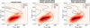 |
Fig. 2 Spectral index distribution simulated disks. The heat map represents the spectral index distribution of the observed disks with the black dots representing each single observed disk. The black and red lines refer to the simulated results for the entire parameter space of initial conditions (Table 2) and the observational results, respectively. The continuous lines encompass the 30% of the cumulative sum of the disks produced from the simulations or observed. The dashed lines encompass the 90% of the cumulative sum of the disks produced from the simulations or observed. We compare our simulated spectral index distributions to the observed sample of Lupus region reported in Tazzari et al. (2021b). The latter is a collection of disks from the Lupus region, detected at 0.89 mm (Ansdell et al. 2016) and 3.1 mm (Tazzari et al. 2021b). Left plot: spectral index distribution simulated smooth disks. Middle plot: spectral index distribution simulated substructured disks with planet randomly inserted in a range between 0.1–0.4 Myr. Right plot: spectral index distribution simulated substructured disks with planet randomly inserted in a range between 0.4–1 Myr. |
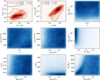 |
Fig. 3 Spectral index, size–luminosity, and initial parameter distributions for the parameter space of the initial conditions selecting disks with a spectral index of 0 ⋦ α0.89-3.1 mm ⋦ 4, 10−3 Jy ⋦ F1 mm ⋦ 10 Jy, 10−3 Jy ⋦ F0.89 mm ⋦ 10 Jy, and 100.1 au ⋦ reff ⋦ 102.6 au. We compare our simulated spectral index distributions to the observed sample of Lupus region reported in Tazzari et al. (2021b). The latter is a collection of disks from the Lupus region, detected at 0.89 mm (Ansdell et al. 2016) and 3.1 mm (Tazzari et al. 2021b). We compare our simulated size–luminosity distribution to the observed sample reported in Andrews et al. (2018b). |
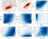 |
Fig. 4 Spectral index, size–luminosity, and initial parameter distributions, selecting disks with a spectral index of α0.89-3.1 mm ≤ 2.5. |
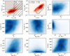 |
Fig. 5 Spectral index, size–luminosity, and initial parameter distributions, selecting disks with a spectral index of α0.89-3.1 mm ≤ 2.5 and a flux of F1 mm ≤ 0.1 Jy. |
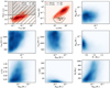 |
Fig. 6 Spectral index, size–luminosity, and initial parameter distributions, selecting disks with a spectral index of α0.89-3.1 mm ≤ 2.5 and a flux of F1 mm ≤ 0.01 Jy. |
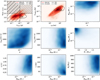 |
Fig. 7 Spectral index, size–luminosity, and initial parameter distributions, selecting disks with a spectral index of α0.89-3.1 mm ≤ 2.5 and a flux of F1 mm > 0.1 Jy. |
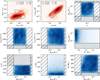 |
Fig. 8 Spectral index, size–luminosity, and initial parameter distributions, selecting disks with 10−3.5 ⩽ α ⩽ 10−2.5, 10−2.3 M⋆ ⩽ Mdisk ⩽ 10−0.5 M⋆, υfrag ≥ 500 cm s−1, mp ≥ 150 M⊕, and rp ≤ 0.75 rc. |
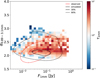 |
Fig. 9 Spectral index and flux-averaged optical depth distribution at 1 mm (τ1 mm), selecting disks with 10−3.5 ⩽ α ⩽ 10−2.5, 10−2.3 M⋆ ⩽ Mdisk ⩽ 10−0.5 M⋆, υfrag ≥ 500 cm s−1, mp ≥ 150 M⊕, and rp ≤ 0.75 rc. The optical depth associated with each bin is the mean of the flux-averaged optical depths of the disks belonging to each bin. |
3.2 Case studies on opacities, the initial mass function, and double substructure
3.2.1 Opacities
All the results shown in the previous section were obtained considering Ricci compact opacities (Rosotti et al. (2019a)). This opacity proved to be the best at reproducing the observed distributions, as has already been noted in Zormpas et al. (2022) and Stadler et al. (2022), for the study of the size–luminosity distribution. Figure 10 shows a comparison between the distributions obtained for the spectral index in the case of three different opacities: Ricci opacity model (Ricci et al. 2010b) with compact grains (Ricci compact model) as in Rosotti et al. (2019a) (0% grain porosity), DSHARP (Birnstiel et al. 2018) with 0% grain porosity, and DIANA (Woitke et al. 2016) (25% grain porosity) opacities. The only model capable of producing disks with a spectral index of ~2.2 is the Ricci compact model. DIANA produces disks with low spectral index values but fails to populate the observed regions at α0.89-3.1 mm ≤ 2.3. DSHARP suffers from the same problem as DIANA and also produces disks with a lower flux that do not reach the observed extent. The latter problem was already highlighted by Zormpas et al. (2022), who also showed that as grain opacity increases, disk flux reduces in the DSHARP case (see Appendix D for an in-depth investigation of different percentages of grain porosity for DSHARP opacities). The difference in the final result between DIANA and Ricci compact lies in the compactness of the grains considered for Ricci. The difference between Ricci and DSHARP, on the other hand, resides in the fact that Ricci’s opacity has a value ~8.5 higher than DHSARP’s at the position of the opacity cliff if, for example, we consider a wavelength of 850 μm. This explains the difference in the final flux value of the disks obtained in the case of Ricci compared to DSHARP.
Disk population synthesis represents a valuable tool that can provide additional insight into the definition of opacity and dust composition models. Dust composition, porosity, and opacity determinations represent one of the main open problems in the field. Indeed, they are crucial hypotheses for determining disk characteristics, but we still lack precise knowledge of both of them. Thus, finding a solution to this problem constitutes a very active field in the protoplanetary disk panorama, which is being addressed through different techniques such as: submillimeter polarization (Kataoka et al. 2016, 2017), the scattered light phase function (Ginski et al. 2023), and multiwavelength studies (Guidi et al. 2022). The multiwavelength study by Guidi et al. (2022) and the scattered light phase function study by Ginski et al. (2023) support the idea of low-porosity grains in protoplanetary disks. In particular, the Guidi et al. (2022) study on grain properties in the ringed disk of HD 163296 shows that low-porosity grains better reproduce the observations of HD 163296. Ginski et al. (2023) show that two categories of aggregates can be associated with polarized phase functions. The first category consists of fractal, porous aggregates, while the second one consists of more compact and less porous aggregates. In particular, they note that disks belonging to the second category host embedded planets that may trigger enhanced vertical mixing, leading to the production of more compact particles. Submillimeter polarization studies (Kataoka et al. 2016, 2017), on the other hand, provide important information about the maximum grain size. They constrain a maximum grain size of ~ 100 μm In an optically thin regime, such grains would not produce a low spectral index value; indeed, α0.89-3.1 ≤ 2.5 requires grains larger than 1mm. However, as Fig. 9 shows, low spectral index values are produced by the presence of an optically thick region caused by substructure.
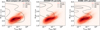 |
Fig. 10 Spectral index distribution simulated substructured disks, for the entire parameter space of initial conditions (Table 2) for three different opacities. The heat map represents the spectral index distribution of the observed disks with the black dots representing each single observed disk. The black and red lines refer to the simulated results and the observational results, respectively. The continuous lines encompass the 30% of the cumulative sum of the disks produced from the simulations or observed. The dashed lines encompass the 90% of the cumulative sum of the disks produced from the simulations or observed. Left plot: spectral index distribution simulated substructured disks. The opacities model adopted for the simulated disks reported in this plot is the Ricci opacity model (Ricci et al. 2010b) with compact grains (Ricci compact model) as in Rosotti et al. (2019a) (0% grain porosity). Middle plot: spectral index distribution simulated substructured disks. The opacities model adopted for the simulated disks reported in this plot is the DSHARP (Birnstiel et al. 2018) model with 0% grain porosity. Right plot: spectral index distribution simulated substructured disks. The opacities model adopted for the simulated disks reported in this plot is the DIANA (Woitke et al. 2016) model (25% grain porosity). |
3.2.2 Initial mass function
As is shown in Table 2, the stellar masses of our simulations were drawn from the functional form of the IMF proposed by Maschberger (2013), which is based on the standard IMFs of Kroupa (Kroupa 2001, 2002) and Chabrier (Chabrier 2003). To make our comparison to the observed disk distributions more consistent, we also accounted for the fact that the observed disks may be characterized by a stellar mass distribution that differs from the standard IMFs of Kroupa and Chabrier. We therefore constructed an IMF from a kernel density estimate derived from the stellar mass distributions of the samples in Tazzari et al. (2021a) and Andrews et al. (2018b). Figure 11 shows that the results obtained with the new IMF deviate only slightly from the classical IMF case, mainly in terms of a slight shift to higher fluxes.
3.2.3 Double substructure
Figure 12 shows a comparison of the behavior of the simulated spectral index distribution when one or two planets (i.e., substructures) are inserted during the evolution of the disk. We analyzed two different scenarios: in the first scenario, the earliest substructure is the innermost one (blue contours); in the second scenario, the earliest substructure is the outermost one (green contours). It can be immediately observed that it is possible to produce spectral index values in the observed region even in the generic case of two substructures. In general, the double substructure distributions are similar to the single substructure case and simply show a shift in the final flux produced. In the case of two substructures and faster insertion of the innermost substructure, the value of the final flux produced is lower than in the case of faster insertion of the outer substructure, as in the latter case there is a greater accumulation of material in the outer region with which a greater area is associated. A brighter disk is therefore generally obtained in the second scenario. The double substructure case, with primary insertion of the innermost substructure, generally produces fainter disks than the single substructure case because a range of rp = 0.05 − 0.5 rc was selected in the double substructure case.
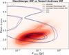 |
Fig. 11 Spectral index distribution simulated substructured disks, for the entire parameter space of initial conditions (Table 2) for two different IMFs. The heat map represents the spectral index distribution of the observed disks with the black dots representing each single observed disk. The black, blue, and red lines refer to the simulated results obtained for the functional form of the IMF proposed by Maschberger 2013 (black), which is based on the standard IMFs of Kroupa (Kroupa 2001, 2002) and Chabrier (Chabrier 2003), as well as the Andrews-Tazzari IMF (blue) and the observational results (red). The continuous lines encompass the 30% of the cumulative sum of the disks produced from the simulations or observed. The dashed lines encompass the 90% of the cumulative sum of the disks produced from the simulations or observed. |
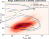 |
Fig. 12 Spectral index distribution simulated substructured disks, for the entire parameter space of initial conditions (Table 2) for disks with one substructure and two substructures. The heat map represents the spectral index distribution of the observed disks with the black dots representing each single observed disk. The black, blue, green, and red lines refer to the simulated results obtained for single substructured disks (black), double substructured disks with the inner planet inserted first (blue), and double substructured disks with the outer planet inserted first (green), as well as the observational results (red). The continuous lines encompass the 30% of the cumulative sum of the disks produced from the simulations or observed. The dashed lines encompass the 90% of the cumulative sum of the disks produced from the simulations or observed. |
3.3 Future perspectives and open problems
In Fig. 13, we investigate the distribution of the spectral index evaluated at longer wavelengths (α3.1-9 mm) for the disk filtered by applying the best cuts introduced in Sec. 3.1. We observe a slight general shift toward larger values for the spectral index, since less of the emitting region produced by the substructure is optically thick and some parts become optically thin while not being made of very large grains. This behavior opens an interesting window onto disk mass estimates, since a search for optically thin emission is required for accurate estimates of disk masses, and thus also to estimate the amount of material available for planet formation. However, at the moment, only a small sample of disks have been observed at large wavelengths; for instance, only around 30 disks have been observed at λ ~ 7.5 mm (mostly by Rodmann et al. 2006; Ubach et al. 2012).
In this study, we have chosen to define our effective radius for the disk size as the radius that encloses the 68% of the total amount of flux produced by the disk (reff,68%,), following Tripathi et al. (2017). Nevertheless, the most recent observations have considered the radius that encloses 90% of the emission (reff,90%). However, Hendler et al. (2020) find a 1–1 correlation between reff,90% and reff,68% (see Fig. 15 in (Hendler et al. 2020)). We have thus evaluated reff,90% for each disk and tested if our population synthesis can reproduce this observed trend. Figure 14 shows the behavior exhibited by three different disk populations: smooth disks, substructured disks without any cut being applied to the initial conditions, and substructured disks filtered with our best conditions (i.e., 10−3.5 ⩽ α ⩽ 10−25, 10−2.3 M⋆ ⩽ Mdisk ⩽ 10−0.5 M⋆, υfrag ≥ 500 cm s−1, mp ≥ 150 M⊕, and rp ≤ 0.75rc). We selected a set of 104 disk per population and fit each sample exploiting linmix implementation of the Bayesian linear regression method developed by Kelly (2007). The results reported in Table 3 show that smooth disks do not reproduce the correlation observed in Hendler et al. (2020); the same applies to the substructured disk population. However, filtering the substructured disk population, selecting disks with 10−3.5 ⩽ α ⩽ 10−25, 10−2.3 M⋆ ⩽ Mdisk ⩽ 10−0.5 M⋆, υfrag ≥ 500 cm s−1, mp ≥ 150M⊕, and rp ≤ 0.75 rc − that is, applying the best cuts introduced in Sec. 3.1 that lead to matching both the spectral index and size–luminosity distribution – we obtain a correlation between log reff,90% and log reff,68%. This result further strengthens the outcomes outlined in Sec. 3.1 concerning the need for substructure in protoplanetary disks and the associated parameter space.
In this work, we have focused on the classical scenario in which disks evolve viscously. However, in recent years, the hypothesis that the evolution of the disk is driven by magnetic winds has become increasingly popular. We therefore aim to expand our investigation on the MHD disk winds scenario in the future, to determine if differences might arise compared to the viscous scenario, and if so what those differences might be. In this respect, Zagaria et al. (2022) show that current available observations do not allow one to discern between viscous and magnetic wind scenarios and that, from the dust perspective, there is little difference between the viscous case and MHD winds. Indeed, they show that SLR can be reproduced even by MHD disk winds models, except for the very large disks, which can, however, be explained by assuming the presence of substructures. We therefore expect, adopting an MHD wind model, similar conclusions to those obtained for the viscous scenario.
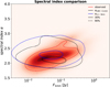 |
Fig. 13 Spectral index distribution simulated substructured disks, selecting simulated disks with: 10−35 ⩽ α ⩽ 10−25, 10−23 M⋆ ⩽ Mdisk ⩽ 10−0.5 M⋆, υfrag ≥ 500 cm s−1, mp ≥ 150 M⊕, and rp ≤ 0 75 rc. The heat map represents the spectral index distribution of the observed disks with the black dots representing each single observed disk. The black, blue, and red lines refer to the simulated results obtained for α0.89-3.1 mm (black), the simulated results obtained for α3.1-9 mm (blue), and the observational results (α0.89-3.1 mm) (red). The continuous lines encompass the 30% of the cumulative sum of the disks produced from the simulations or observed. The dashed lines encompass the 90% of the cumulative sum of the disks produced from the simulations or observed. |
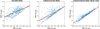 |
Fig. 14 Comparison between log reff,90% and log reff,68% dust disk sizes for smooth disks (left panel), an entire set of substructured disks (middle panel), and substructured disks selected from our best case (i.e., 10−3.5 ⩽ α ⩽ 10−2.5, 10−2.3 M⋆ ⩽ Mdisk ⩽ 10−0.5 M⋆, υfrag ≥ 500 cm s−1, mp ≥ 150 M⊕, and rp ≤ 0.75 rc) (right plot). Blue dots represent a subset of the disks used in the estimate of the correlation between reff,90% and reff,68%. The best fit obtained exploiting the linmix implementation of the Bayesian linear regression method developed by Kelly (2007) is shown as a black line, with a 1σ confidence interval reported in red. |
log reff,90% vs. log reff,68% fit results.
4 Conclusions
In this work, we conducted a study aimed at understanding the possibility of reproducing the observed spectral index distribution of protoplanetary disks. We exploited the two-pop-py 1D evolutionary model for the dust and gas in protoplanetary disks. We considered both smooth and substructured disks and a wide initial parameter space. We firstly compared the simulated distribution obtained for the spectral index to the observed ones reported in Tazzari et al. (2021b) and then analyzed the possibility of also matching the size–luminosity distribution, considering the observed distribution reported in Andrews et al. (2018b). We have been able to identify the initial conditions and the kind of disks needed to match the spectral index distribution and in particular to also simultaneously match the size–luminosity distribution. These are the main results that we have outlined:
- 1.
Substructures are needed to produce small values of the spectral index in the range of the observed ones; smooth disks only produce large values of the spectral index (Fig. 2);
- 2.
The substructure has to be formed quickly – that is, within ~0.4 Myr (Fig. 2) – to produce a value of spectral index below 2.5;
- 3.
Filtering the substructure disks with 10−3.5 ⩽ α ⩽ 10−2.5, 10−2.3 M⋆ ⩽ Mdisk ⩽ 10−0.5 M⋆, υfrag ≥ 500 cm s−1, mp ≥ 150 M⊕, and rp ≤ 0.75rc, we obtain a match between the spectral index simulated distribution and the observed distribution (Fig. 8), proving that it is possible to reproduce the observed distribution for a reasonable range of initial conditions;
- 4.
An in-depth investigation of the real cause behind the production of low spectral index values for substructured disks revealed that this is achieved by the production of an optically thick region in the disk, originating from the accumulation of material due to the presence of substructure;
- 5.
The matching obtained between the simulated and observed spectral index distribution automatically ensures a match between the corresponding simulated and observed size–luminosity distribution;
- 6.
It is possible to reproduce the size–luminosity distribution with a population of only substructured disks, and thus the mix of smooth and substructured disks proposed in Zormpas et al. (2022) is no longer required;
- 7.
The 1–1 correlation between the reff,90% and reff,68% observed in Hendler et al. (2020) cannot be reproduced by smooth disks and by the entire sample of substructured disks, but can be retrieved by filtering the substructured disk sample with the same parameter ranges that lead to both the spectral index and size–luminosity distributions being reproduced;
- 8.
Studying different opacities (Ricci compact Rosotti et al. 2019a, DSHARP Birnstiel et al. 2018, and DIANA Woitke et al. 2016) we have shown that the only one capable of leading to a match with the spectral index distribution is the Ricci compact opacity. Only opacities with a high absorption efficiency can reproduce the observed spectral indices;
- 9.
Disks with two substructures can match the spectral index distribution, showing a behavior similar to the single substructure case.
This study shows that it is possible to reproduce the observed distributions for both the spectral index and size–luminosity, extending the results obtained for individual disk studies to the broader level of a disk population synthesis.
Acknowledgements
L.D. and T.B. acknowledge funding by the Deutsche Forschungsgemeinschaft (DFG, German Research Foundation) under grant 325594231 and Germany’s Excellence Strategy – EXC-2094 – 390783311. T.B. acknowledges funding from the European Research Council (ERC) under the European Union’s Horizon 2020 research and innovation programme under grant agreement No 714769. P.P. acknowledges funding from the UK Research and Innovation (UKRI) under the UK government’s Horizon Europe funding guarantee from ERC (under grant agreement no 101076489). GR acknowledges funding from the Fondazione Cariplo, grant no. 2022-1217, and the European Research Council (ERC) under the European Union’s Horizon Europe Research & Innovation Programme under grant agreement no. 101039651 (DiscEvol). Views and opinions expressed are however those of the author(s) only, and do not necessarily reflect those of the European Union or the European Research Council Executive Agency. Neither the European Union nor the granting authority can be held responsible for them.
Appendix A Evolving Lstar versus fixed Lstar
In this appendix, we show the comparison between the spectral index simulated distribution obtained for a scenario in which we keep the luminosity of the hosting star fixed and the scenario in which we let L⋆ evolve over time.
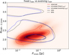 |
Fig. A.1 Spectral index distribution simulated substructured disks, for the entire parameter space of initial conditions (Table 2), for the scenario in which we keep Lstar fixed during the disk evolution (black lines) and the scenario in which Lstar evolves over time. The heat map represents the spectral index distribution of the observed disks with the black dots representing each single observed disk. The black, blue, and red lines refer to the simulated results obtained for a fixed Lstar (black), simulated results obtained for an evolving Lstar (blue), and the observational results (red). The continuous lines encompass the 30% of the cumulative sum of the disks produced from the simulations or observed. The dashed lines encompass the 90% of the cumulative sum of the disks produced from the simulations or observed. |
Appendix B Initial parameter distributions
In this appendix, we show the spectral index, size–luminosity, and initial parameter distributions for the entire parameter space of initial conditions (see Table 2).
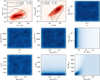 |
Fig. B.1 Spectral index, size–luminosity, and initial parameter distributions for the entire parameter space of initial conditions. We compare our simulated spectral index distributions to the observed sample of Lupus region reported in Tazzari et al. (2021b). The latter is a collection of disks from the Lupus region, detected at 0.89mm (Ansdell et al. 2016) and 3.1mm (Tazzari et al. 2021b). We compare our simulated SLR to the observed sample reported in Andrews et al. (2018b). |
Appendix C Size-luminosity diagram analysis
In this appendix, we show the spectral index, size–luminosity, and initial parameter distributions selecting disks populating two different regions in the size–luminosity diagram.
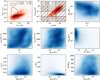 |
Fig. C.1 Spectral index, size–luminosity, and initial parameter distributions selecting disks with 0.8 ⩽ log reff[au] ⩽ 1.6 and −2 ⩽ log F0.89mm[Jy] ⩽ −1. |
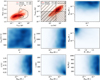 |
Fig. C.2 Spectral index, size–luminosity, and initial parameter distributions selecting disks with 1.6 ⩽ log reff[au] ⩽ 2.5 and −1 ⩽ log F0.89mm[Jy] ⩽ 0.5. |
Appendix D DSHARP opacities for different percentages of grain porosity
In this appendix, we show the comparison between the spectral index simulated distribution obtained for DHSARP opacities (Birnstiel et al. 2018) for different percentages of grain porosity.
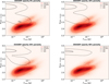 |
Fig. D.1 Spectral index distribution simulated substructured disks, for the entire parameter space of initial conditions (Table 2) for DSHARP opacities model (Birnstiel et al. 2018), for four different percentages of grain porosity. The heat map represents the spectral index distribution of the observed disks with the black dots representing each single observed disk. The black and red lines refer to the simulated results and the observational results, respectively. The continuous lines encompass the 30% of the cumulative sum of the disks produced from the simulations or observed. The dashed lines encompass the 90% of the cumulative sum of the disks produced from the simulations or observed. |
References
- Andrews, S. M., Rosenfeld, K. A., Kraus, A. L., & Wilner, D. J. 2013, ApJ, 771, 129 [Google Scholar]
- Andrews, S. M., Huang, J., Pérez, L. M., et al. 2018a, ApJ, 869, L41 [NASA ADS] [CrossRef] [Google Scholar]
- Andrews, S. M., Terrell, M., Tripathi, A., et al. 2018b, ApJ, 865, 157 [Google Scholar]
- Ansdell, M., Williams, J. P., van der Marel, N., et al. 2016, ApJ, 828, 46 [Google Scholar]
- Bai, X.-N., & Stone, J. M. 2014, ApJ, 796, 31 [Google Scholar]
- Birnstiel, T., Dullemond, C. P., & Brauer, F. 2010, A&A, 513, A79 [NASA ADS] [CrossRef] [EDP Sciences] [Google Scholar]
- Birnstiel, T., Klahr, H., & Ercolano, B. 2012, A&A, 539, A148 [NASA ADS] [CrossRef] [EDP Sciences] [Google Scholar]
- Birnstiel, T., Andrews, S. M., Pinilla, P., & Kama, M. 2015, ApJ, 813, L14 [NASA ADS] [CrossRef] [Google Scholar]
- Birnstiel, T., Dullemond, C. P., Zhu, Z., et al. 2018, ApJ, 869, L45 [CrossRef] [Google Scholar]
- Chabrier, G. 2003, PASP, 115, 763 [Google Scholar]
- D’Alessio, P., Calvet, N., Hartmann, L., Franco-Hernández, R., & Servín, H. 2006, ApJ, 638, 314 [Google Scholar]
- Draine, B. 2006, ApJ, 636, 1114 [NASA ADS] [CrossRef] [Google Scholar]
- Ginski, C., Tazaki, R., Dominik, C., & Stolker, T. 2023, ApJ, 953, 92 [NASA ADS] [CrossRef] [Google Scholar]
- Guidi, G., Isella, A., Testi, L., et al. 2022, A&A, 664, A137 [NASA ADS] [CrossRef] [EDP Sciences] [Google Scholar]
- Hendler, N., Pascucci, I., Pinilla, P., et al. 2020, ApJ, 895, 126 [Google Scholar]
- Huang, J., Andrews, S. M., Dullemond, C. P., et al. 2018, ApJ, 869, L42 [NASA ADS] [CrossRef] [Google Scholar]
- Izquierdo, A. F., Facchini, S., Rosotti, G. P., van Dishoeck, E. F., & Testi, L. 2022, ApJ, 928, 2 [NASA ADS] [CrossRef] [Google Scholar]
- Johansen, A., Youdin, A., & Klahr, H. 2009, ApJ, 697, 1269 [Google Scholar]
- Kanagawa, K. D., Muto, T., Tanaka, H., et al. 2016, PASJ, 68, 43 [NASA ADS] [Google Scholar]
- Kataoka, A., Muto, T., Momose, M., et al. 2015, ApJ, 809, 78 [Google Scholar]
- Kataoka, A., Tsukagoshi, T., Momose, M., et al. 2016, ApJ, 831, L12 [Google Scholar]
- Kataoka, A., Tsukagoshi, T., Pohl, A., et al. 2017, ApJ, 844, L5 [Google Scholar]
- Kelly, B. C. 2007, ApJ, 665, 1489 [Google Scholar]
- Kenyon, S. J., Yi, I., & Hartmann, L. 1996, ApJ, 462, 439 [NASA ADS] [CrossRef] [Google Scholar]
- Keppler, M., Benisty, M., Müller, A., et al. 2018, A&A, 617, A44 [NASA ADS] [CrossRef] [EDP Sciences] [Google Scholar]
- Kroupa, P. 2001, MNRAS, 322, 231 [NASA ADS] [CrossRef] [Google Scholar]
- Kroupa, P. 2002, Science, 295, 82 [Google Scholar]
- Long, F., Pinilla, P., Herczeg, G. J., et al. 2018, ApJ, 869, 17 [Google Scholar]
- Lüst, R. 1952, Zeitsch. Naturf. A, 7, 87 [CrossRef] [Google Scholar]
- Lynden-Bell, D., & Pringle, J. E. 1974, MNRAS, 168, 603 [Google Scholar]
- Manara, C., Rosotti, G., Testi, L., et al. 2016, A&A, 591, A3 [NASA ADS] [CrossRef] [EDP Sciences] [Google Scholar]
- Manara, C. F., Ansdell, M., Rosotti, G. P., et al. 2023, Protostars and Planets VII, eds. S. Inutsuka, Y. Aikawa, T. Muto, K. Tomida, & M. Tamura, ASP Conf. Ser., 534, 539 [NASA ADS] [Google Scholar]
- Maschberger, T. 2013, MNRAS, 429, 1725 [NASA ADS] [CrossRef] [Google Scholar]
- Miotello, A., Kamp, I., Birnstiel, T., Cleeves, L., & Kataoka, A. 2023, ASP Conf. Ser., 534, 501 [NASA ADS] [Google Scholar]
- Miyake, K., & Nakagawa, Y. 1993, Icarus, 106, 20 [NASA ADS] [CrossRef] [Google Scholar]
- Müller, A., Keppler, M., Henning, T., et al. 2018, A&A, 617, A2 [Google Scholar]
- Natta, A., Testi, L., Johnstone, D., et al. 2004, in ASP Conf. Proc., 323, 279 [NASA ADS] [Google Scholar]
- Okuzumi, S., Momose, M., Sirono, S.-i., Kobayashi, H., & Tanaka, H. 2016, ApJ, 821, 82 [Google Scholar]
- Paardekooper, S. J., & Mellema, G. 2004, A&A, 425, L9 [NASA ADS] [CrossRef] [EDP Sciences] [Google Scholar]
- Pascucci, I., Testi, L., Herczeg, G. J., et al. 2016, ApJ, 831, 125 [Google Scholar]
- Pinilla, P., Benisty, M., & Birnstiel, T. 2012a, A&A, 545, A81 [NASA ADS] [CrossRef] [EDP Sciences] [Google Scholar]
- Pinilla, P., Birnstiel, T., Ricci, L., et al. 2012b, A&A, 538, A114 [NASA ADS] [CrossRef] [EDP Sciences] [Google Scholar]
- Pinilla, P., Pohl, A., Stammler, S. M., & Birnstiel, T. 2017, ApJ, 845, 68 [Google Scholar]
- Pinte, C., Price, D. J., Ménard, F., et al. 2018, ApJ, 860, L13 [Google Scholar]
- Pollack, J. B., Hollenbach, D., Beckwith, S., et al. 1994, ApJ, 421, 615 [Google Scholar]
- Pollack, J. B., Hubickyj, O., Bodenheimer, P., et al. 1996, Icarus, 124, 62 [NASA ADS] [CrossRef] [Google Scholar]
- Ragusa, E., Dipierro, G., Lodato, G., Laibe, G., & Price, D. J. 2017, MNRAS, 464, 1449 [Google Scholar]
- Ricci, L., Testi, L., Natta, A., & Brooks, K. 2010a, A&A, 521, A66 [NASA ADS] [CrossRef] [EDP Sciences] [Google Scholar]
- Ricci, L., Testi, L., Natta, A., et al. 2010b, A&A, 512, A15 [CrossRef] [EDP Sciences] [Google Scholar]
- Rice, W. K. M., Armitage, P. J., Wood, K., & Lodato, G. 2006, MNRAS, 373, 1619 [Google Scholar]
- Rodmann, J., Henning, T., Chandler, C., Mundy, L., & Wilner, D. 2006, A&A, 446, 211 [NASA ADS] [CrossRef] [EDP Sciences] [Google Scholar]
- Rosotti, G. P., Booth, R. A., Tazzari, M., et al. 2019a, MNRAS, 486, L63 [Google Scholar]
- Rosotti, G. P., Tazzari, M., Booth, R. A., et al. 2019b, MNRAS, 486, 4829 [NASA ADS] [CrossRef] [Google Scholar]
- Savvidou, S., & Bitsch, B. 2023, A&A, 679, A42 [NASA ADS] [CrossRef] [EDP Sciences] [Google Scholar]
- Shakura, N. I., & Sunyaev, R. A. 1973, A&A, 24, 337 [NASA ADS] [Google Scholar]
- Shi, J.-M., Krolik, J. H., Lubow, S. H., & Hawley, J. F. 2012, ApJ, 749, 118 [Google Scholar]
- Siess, L., Dufour, E., & Forestini, M. 2000, A&A, 358, 593 [Google Scholar]
- Stadler, J., Gárate, M., Pinilla, P., et al. 2022, A&A, 668, A104 [NASA ADS] [CrossRef] [EDP Sciences] [Google Scholar]
- Tazzari, M., Clarke, C. J., Testi, L., et al. 2021a, MNRAS, 506, 2804 [NASA ADS] [CrossRef] [Google Scholar]
- Tazzari, M., Testi, L., Natta, A., et al. 2021b, MNRAS, 506, 5117 [NASA ADS] [CrossRef] [Google Scholar]
- Teague, R., Bae, J., Bergin, E. A., Birnstiel, T., & Foreman-Mackey, D. 2018, ApJ, 860, L12 [NASA ADS] [CrossRef] [Google Scholar]
- Tripathi, A., Andrews, S. M., Birnstiel, T., & Wilner, D. J. 2017, ApJ, 845, 44 [Google Scholar]
- Ubach, C., Maddison, S. T., Wright, C. M., et al. 2012, MNRAS, 425, 3137 [NASA ADS] [CrossRef] [Google Scholar]
- Woitke, P., Min, M., Pinte, C., et al. 2016, A&A, 586, A103 [NASA ADS] [CrossRef] [EDP Sciences] [Google Scholar]
- Youdin, A. N., & Lithwick, Y. 2007, Icarus, 192, 588 [NASA ADS] [CrossRef] [Google Scholar]
- Zagaria, F., Rosotti, G. P., Clarke, C. J., & Tabone, B. 2022, MNRAS, 514, 1088 [CrossRef] [Google Scholar]
- Zhu, Z., Nelson, R. P., Dong, R., Espaillat, C., & Hartmann, L. 2012, ApJ, 755, 6 [Google Scholar]
- Zormpas, A., Birnstiel, T., Rosotti, G. P., & Andrews, S. M. 2022, A&A, 661, A66 [NASA ADS] [CrossRef] [EDP Sciences] [Google Scholar]
All Tables
All Figures
|
Fig. 1 Disk population study procedure. |
| In the text | |
|
Fig. 2 Spectral index distribution simulated disks. The heat map represents the spectral index distribution of the observed disks with the black dots representing each single observed disk. The black and red lines refer to the simulated results for the entire parameter space of initial conditions (Table 2) and the observational results, respectively. The continuous lines encompass the 30% of the cumulative sum of the disks produced from the simulations or observed. The dashed lines encompass the 90% of the cumulative sum of the disks produced from the simulations or observed. We compare our simulated spectral index distributions to the observed sample of Lupus region reported in Tazzari et al. (2021b). The latter is a collection of disks from the Lupus region, detected at 0.89 mm (Ansdell et al. 2016) and 3.1 mm (Tazzari et al. 2021b). Left plot: spectral index distribution simulated smooth disks. Middle plot: spectral index distribution simulated substructured disks with planet randomly inserted in a range between 0.1–0.4 Myr. Right plot: spectral index distribution simulated substructured disks with planet randomly inserted in a range between 0.4–1 Myr. |
| In the text | |
|
Fig. 3 Spectral index, size–luminosity, and initial parameter distributions for the parameter space of the initial conditions selecting disks with a spectral index of 0 ⋦ α0.89-3.1 mm ⋦ 4, 10−3 Jy ⋦ F1 mm ⋦ 10 Jy, 10−3 Jy ⋦ F0.89 mm ⋦ 10 Jy, and 100.1 au ⋦ reff ⋦ 102.6 au. We compare our simulated spectral index distributions to the observed sample of Lupus region reported in Tazzari et al. (2021b). The latter is a collection of disks from the Lupus region, detected at 0.89 mm (Ansdell et al. 2016) and 3.1 mm (Tazzari et al. 2021b). We compare our simulated size–luminosity distribution to the observed sample reported in Andrews et al. (2018b). |
| In the text | |
|
Fig. 4 Spectral index, size–luminosity, and initial parameter distributions, selecting disks with a spectral index of α0.89-3.1 mm ≤ 2.5. |
| In the text | |
|
Fig. 5 Spectral index, size–luminosity, and initial parameter distributions, selecting disks with a spectral index of α0.89-3.1 mm ≤ 2.5 and a flux of F1 mm ≤ 0.1 Jy. |
| In the text | |
|
Fig. 6 Spectral index, size–luminosity, and initial parameter distributions, selecting disks with a spectral index of α0.89-3.1 mm ≤ 2.5 and a flux of F1 mm ≤ 0.01 Jy. |
| In the text | |
|
Fig. 7 Spectral index, size–luminosity, and initial parameter distributions, selecting disks with a spectral index of α0.89-3.1 mm ≤ 2.5 and a flux of F1 mm > 0.1 Jy. |
| In the text | |
|
Fig. 8 Spectral index, size–luminosity, and initial parameter distributions, selecting disks with 10−3.5 ⩽ α ⩽ 10−2.5, 10−2.3 M⋆ ⩽ Mdisk ⩽ 10−0.5 M⋆, υfrag ≥ 500 cm s−1, mp ≥ 150 M⊕, and rp ≤ 0.75 rc. |
| In the text | |
|
Fig. 9 Spectral index and flux-averaged optical depth distribution at 1 mm (τ1 mm), selecting disks with 10−3.5 ⩽ α ⩽ 10−2.5, 10−2.3 M⋆ ⩽ Mdisk ⩽ 10−0.5 M⋆, υfrag ≥ 500 cm s−1, mp ≥ 150 M⊕, and rp ≤ 0.75 rc. The optical depth associated with each bin is the mean of the flux-averaged optical depths of the disks belonging to each bin. |
| In the text | |
|
Fig. 10 Spectral index distribution simulated substructured disks, for the entire parameter space of initial conditions (Table 2) for three different opacities. The heat map represents the spectral index distribution of the observed disks with the black dots representing each single observed disk. The black and red lines refer to the simulated results and the observational results, respectively. The continuous lines encompass the 30% of the cumulative sum of the disks produced from the simulations or observed. The dashed lines encompass the 90% of the cumulative sum of the disks produced from the simulations or observed. Left plot: spectral index distribution simulated substructured disks. The opacities model adopted for the simulated disks reported in this plot is the Ricci opacity model (Ricci et al. 2010b) with compact grains (Ricci compact model) as in Rosotti et al. (2019a) (0% grain porosity). Middle plot: spectral index distribution simulated substructured disks. The opacities model adopted for the simulated disks reported in this plot is the DSHARP (Birnstiel et al. 2018) model with 0% grain porosity. Right plot: spectral index distribution simulated substructured disks. The opacities model adopted for the simulated disks reported in this plot is the DIANA (Woitke et al. 2016) model (25% grain porosity). |
| In the text | |
|
Fig. 11 Spectral index distribution simulated substructured disks, for the entire parameter space of initial conditions (Table 2) for two different IMFs. The heat map represents the spectral index distribution of the observed disks with the black dots representing each single observed disk. The black, blue, and red lines refer to the simulated results obtained for the functional form of the IMF proposed by Maschberger 2013 (black), which is based on the standard IMFs of Kroupa (Kroupa 2001, 2002) and Chabrier (Chabrier 2003), as well as the Andrews-Tazzari IMF (blue) and the observational results (red). The continuous lines encompass the 30% of the cumulative sum of the disks produced from the simulations or observed. The dashed lines encompass the 90% of the cumulative sum of the disks produced from the simulations or observed. |
| In the text | |
|
Fig. 12 Spectral index distribution simulated substructured disks, for the entire parameter space of initial conditions (Table 2) for disks with one substructure and two substructures. The heat map represents the spectral index distribution of the observed disks with the black dots representing each single observed disk. The black, blue, green, and red lines refer to the simulated results obtained for single substructured disks (black), double substructured disks with the inner planet inserted first (blue), and double substructured disks with the outer planet inserted first (green), as well as the observational results (red). The continuous lines encompass the 30% of the cumulative sum of the disks produced from the simulations or observed. The dashed lines encompass the 90% of the cumulative sum of the disks produced from the simulations or observed. |
| In the text | |
|
Fig. 13 Spectral index distribution simulated substructured disks, selecting simulated disks with: 10−35 ⩽ α ⩽ 10−25, 10−23 M⋆ ⩽ Mdisk ⩽ 10−0.5 M⋆, υfrag ≥ 500 cm s−1, mp ≥ 150 M⊕, and rp ≤ 0 75 rc. The heat map represents the spectral index distribution of the observed disks with the black dots representing each single observed disk. The black, blue, and red lines refer to the simulated results obtained for α0.89-3.1 mm (black), the simulated results obtained for α3.1-9 mm (blue), and the observational results (α0.89-3.1 mm) (red). The continuous lines encompass the 30% of the cumulative sum of the disks produced from the simulations or observed. The dashed lines encompass the 90% of the cumulative sum of the disks produced from the simulations or observed. |
| In the text | |
|
Fig. 14 Comparison between log reff,90% and log reff,68% dust disk sizes for smooth disks (left panel), an entire set of substructured disks (middle panel), and substructured disks selected from our best case (i.e., 10−3.5 ⩽ α ⩽ 10−2.5, 10−2.3 M⋆ ⩽ Mdisk ⩽ 10−0.5 M⋆, υfrag ≥ 500 cm s−1, mp ≥ 150 M⊕, and rp ≤ 0.75 rc) (right plot). Blue dots represent a subset of the disks used in the estimate of the correlation between reff,90% and reff,68%. The best fit obtained exploiting the linmix implementation of the Bayesian linear regression method developed by Kelly (2007) is shown as a black line, with a 1σ confidence interval reported in red. |
| In the text | |
|
Fig. A.1 Spectral index distribution simulated substructured disks, for the entire parameter space of initial conditions (Table 2), for the scenario in which we keep Lstar fixed during the disk evolution (black lines) and the scenario in which Lstar evolves over time. The heat map represents the spectral index distribution of the observed disks with the black dots representing each single observed disk. The black, blue, and red lines refer to the simulated results obtained for a fixed Lstar (black), simulated results obtained for an evolving Lstar (blue), and the observational results (red). The continuous lines encompass the 30% of the cumulative sum of the disks produced from the simulations or observed. The dashed lines encompass the 90% of the cumulative sum of the disks produced from the simulations or observed. |
| In the text | |
|
Fig. B.1 Spectral index, size–luminosity, and initial parameter distributions for the entire parameter space of initial conditions. We compare our simulated spectral index distributions to the observed sample of Lupus region reported in Tazzari et al. (2021b). The latter is a collection of disks from the Lupus region, detected at 0.89mm (Ansdell et al. 2016) and 3.1mm (Tazzari et al. 2021b). We compare our simulated SLR to the observed sample reported in Andrews et al. (2018b). |
| In the text | |
|
Fig. C.1 Spectral index, size–luminosity, and initial parameter distributions selecting disks with 0.8 ⩽ log reff[au] ⩽ 1.6 and −2 ⩽ log F0.89mm[Jy] ⩽ −1. |
| In the text | |
|
Fig. C.2 Spectral index, size–luminosity, and initial parameter distributions selecting disks with 1.6 ⩽ log reff[au] ⩽ 2.5 and −1 ⩽ log F0.89mm[Jy] ⩽ 0.5. |
| In the text | |
|
Fig. D.1 Spectral index distribution simulated substructured disks, for the entire parameter space of initial conditions (Table 2) for DSHARP opacities model (Birnstiel et al. 2018), for four different percentages of grain porosity. The heat map represents the spectral index distribution of the observed disks with the black dots representing each single observed disk. The black and red lines refer to the simulated results and the observational results, respectively. The continuous lines encompass the 30% of the cumulative sum of the disks produced from the simulations or observed. The dashed lines encompass the 90% of the cumulative sum of the disks produced from the simulations or observed. |
| In the text | |
Current usage metrics show cumulative count of Article Views (full-text article views including HTML views, PDF and ePub downloads, according to the available data) and Abstracts Views on Vision4Press platform.
Data correspond to usage on the plateform after 2015. The current usage metrics is available 48-96 hours after online publication and is updated daily on week days.
Initial download of the metrics may take a while.